
Abstract
A gas breakthrough in saturated bentonite is relevant to the safety of high-level radioactive waste repositories. The study of gas transport mechanisms in saturated bentonite is very important for the safety assessment of repositories. This paper proposed a coupled fluid-mechanical interaction model for predicting and simulating the path of gas transport and gas breakthrough in saturated Gaomiaozi bentonite. The model considered the effect of deformation and damage of bentonite on its permeability and introduced pore pressure into the deformation equation of bentonite. The damage coefficient was also introduced into the permeability evolution equation by combining the Mohr–Coulomb criterion, the maximum tensile stress criterion and the damage evolution. In addition, considering the heterogeneity of the soil, the Weibull distribution function was introduced to assign differential values to material parameters of the cells in the model. The numerical simulation of the bentonite stress field and seepage field was realized by the joint MATLAB and COMSOL secondary development, and the evolution law of the pore path in bentonite was explored under a flexible boundary. The gas breakthrough pressure and permeability pressures were calculated at various gas injection from a gas injection experiment into bentonite with flexible boundaries. Finally, the rationality and applicability of the model were verified by comparing the numerically calculated gas breakthrough pressure and permeability with experimental values.
Article highlights
-
1.
This paper proposed a coupled fluid-mechanical interaction model for predicting and simulating the path of gas transport and gas breakthrough in saturated Gaomiaozi bentonite. The model considerd the effect of deformation and damage of bentonite on its permeability and introduced pore pressure into the deformation equation of bentonite.
-
2.
The numerical simulation of the bentonite stress field and seepage field was realized by the joint MATLAB and COMSOL secondary development, and the evolution law of the pore path in bentonite was explored under a flexible boundary.
-
3.
Permeability experiments were carried out on bentonite to obtain the law of gas transportation in bentonite. Combined with experimental analysis, the mechanism of gas migration and breakthrough in bentonite was theoretically deduced.
1 Introduction
With the worldwide depletion of coal and oil resources, the development of nuclear energy is becoming more prominent. The large amount of radioactive waste generated by nuclear power plants has posed a potential threat to environmental protection. Internationally, it is common to bury high-level radioactive waste in a stable stratum of 500–1000 m underground. The repository generally adopts a multi-barrier structure, consisting of nuclear waste, waste containers, buffer material and surrounding rock from the inside to the outside, as shown in Fig. 1. Over time, the bentonite gradually becomes saturated under the action of groundwater (Guo et al. 2022; Tang et al. 2022; Ramesh and Thyagaraj 2022; Liu et al. 2020). Due to the corrosion of waste tanks and the decomposition of microorganisms, gas will be produced in the repository, and the increase in gas pressure will have a greater impact on the safety and stability of the entire repository. Therefore, there is an urgent need to carry out research on gas transport laws within saturated bentonite.

The repository of multi-barrier structure
In many researchers (Cui et al. 2022; Harrington et al. 2012; Ye et al. 2014) the process of gas transport was divided into four stages in saturated bentonite: the dissolution and diffusion stage, gas–water two-phase flow stage, dilatancy control flow stage and macroscopic fracture control flow stage. Domestic and foreign scholars mainly focus on latter two stages, still with some debates. Regarding these two migration mechanisms, the models established by scholars included traditional two-phase flow model, two-phase flow model considering soil deformation and coupling model of two-phase flow model with embedded cracks.
Some researches (Guo and Fall 2021; Leupin et al. 2021; Liu et al. 2021) established a two-phase flow model without considering soil deformation, which was used to simulate the process of gas-driven water in saturated bentonite. The results showed that gas breakthrough occured when the injection pressure approached the critical value of the capillary pressure. Since these models do not consider the deformation of the soil t, there are limitations in simulating the process of permeability change. Many studies (Gutierrez-Rodrigo et al. 2015; Guo and Fall 2018; Guo and Fall 2021; Graham et al. 2012) showed that the effect of dilatancy on gas migration was more significant under most conditions. Some scholars (Ye et al. 2014; Xu et al. 2013) have established the piecewise function of permeability and gas pressure or soil strain. When permeability depended on gas injection pressure, the permeability changed slightly at lower injection pressures and rapidly if the injection pressure was above a predefined threshold. While permeability depended on soil strain (Tawara et al. 2014; Alonso et al. 2012), the permeability was determined by the deformation of the soil, indicating elastic and plastic strains increased significantly when plastic strains were generated in the soil. Some other scholars (Gonzalez-Blanco et al. 2016; Arnedo et al. 2014; Ohno et al. 2022; Olivella and Alonso 2008; Gerard et al. 2014) have introduced embedded fractures in the model. However, these fissures were hypothetical, and they only change properties of the pore pressure and do not incorporate the volume of the fracture independently into the governing equations. However, the expansion process of the prefabricated pore needs to be considered in the model. The process of gas migration through bentonite is more likely to be simulated by the pore expansion model.
The increase in gas injection pressure decreases the elastic modulus and changes the hydraulic characteristics of the soil. In order to simulate the effect of bentonite damage on the elastic modulus and hydraulic characteristics of the soil, a model for the coupling of fluid flow and soil stress will be established, and the difference in the stress–strain relationship will be considered before and after soil damage. In addition, considering the heterogeneity of bentonite, the Weibull distribution will be introduced to generate the distribution of soil elastic modulus and permeability. Then, further exploration of the evolution law of pore expansion in bentonite will be analyzed with gas injection pressure, gas migration law, and the gas breakthrough mechanism in bentonite.
2 Fluid-mechanical interaction model considering bentonite damage
The fluid-mechanical interaction model for gas migration in bentonite is composed of governing equations and the corresponding boundary conditions. The governing equations include the continuous equation, the momentum equation of seepage field and stress field, the evolution equation of soil damage, and the coupling equation of seepage field and stress field.
2.1 The control equation of bentonite deformation
Considering the stress acting on the bentonite by pore pressure, the relationship between stress and strain of bentonite under an axisymmetric boundary can be expressed as Eq. (1).
The geometric equation can be simplified as Eq. (2).
The momentum conservation equation can be simplified as Eq. (3).
2.2 Evolution model of porosity
The Lagrange method was applied to describe the variation of soil porosity. The pore volume and skeleton volume of the element could be obtained by Eqs. (4), (5) and (6).
And
To calculate the material derivative of Eqs. (5), (6) could be obtained.,
Assuming that the deformation of the skeleton was much smaller than the deformation of the pores, \(\frac{{D\left( {\delta V_{s} } \right)}}{Dt} = 0\), and Eq. (6) could be simplified as Eq. (7).
Based on the theory of continuous medium mechanics, the material derivative of the volume element \(\delta V\) could be calculated by Eq. (8).
where the upper symbol “\(\cdot\)” indicates the partial derivative of physical quantity with respect to time,
Substituting Eq. (8) into Eqs. (7), (10) could be obtained.
Through Eq. (11),
Equation (10) could be changed to Eq. (12).
Adding the first three equations in Eqs. (1), (13) could be obtained.
Equation (13) could be modified as Eq. (14).
Substituting Eq. (14) into Eqs. (12), (15) could be obtained.
\(v_{i}^{s}\) (\(i\) = 1, 2, 3) is the velocity component of the soil skeleton. Equation (15) could be rewritten as Eq. (16), which is the evolution equation of soil porosity.
Considering that the motion velocity of the soil skeleton was extremely small, Eq. (16) could be simplified as Eq. (17).
Integrating Eq. (17), we obtained Eq. (18).
where \(\sigma_{rr}^{0}\),\(\sigma_{\theta \theta }^{0}\),\(\sigma_{zz}^{0}\) and \(p_{g0}\) are normal stress in the radial direction, normal stress in the circumferential direction, normal stress in the axial direction and gas pressure in pores at the initial moment, respectively.
\(\phi < < 1\), so there was the following approximate relationship,
Substituting Eq. (19) into Eqs. (18), (20) could be obtained.
\(\frac{1}{3H}\left[ {\left( {\sigma_{rr}^{{}} - \sigma_{rr}^{0} } \right) + \left( {\sigma_{\theta \theta }^{{}} - \sigma_{\theta \theta }^{0} } \right) + \left( {\sigma_{zz}^{{}} - \sigma_{zz}^{0} } \right) - 3\eta \left( {p_{g}^{{}} - p_{g0}^{{}} } \right)} \right] = 1\), Eq. (21) could be obtained.
Substituting Eq. (21) into Eq. (20), we got
2.3 The gas flow equation
The continuity equation for the flow of gas in bentonite can be derived based on the material description.
The mass of gas in volume element \(\delta V\) is \(\delta M_{{\text{g}}}^{{}} = \rho_{{\text{g}}}^{{}} \phi \delta V = m_{{\text{g}}}^{{}} \delta V\). According to the principle of mass conservation, Eq. (23) could be obtained.
\(m_{{\text{g}}}^{{}}\) and \(\rho_{{\text{g}}}\) are mass concentration and mass density of the gas in the soil, we got Eq. (24).
\(v_{g}\) and \(q_{g}\) are the seepage velocity and permeability velocity of the gas, and Eq. (25) could be obtained.
where, \(v_{gr}\) and \(v_{gz}\) are radial and axial components of seepage velocity. \(q_{gr}\) and \(q_{gz}\) are radial and axial components of permeability velocity.
Expanding the left side of Eq. (23), we got
The right side of Eq. (26) could be expressed as Eq. (27).
Substituting Eq. (24) into Eqs. (27), (28) could be got.
Substituting Eq. (28) into Eq. (23), we got
Assuming that the flow of gas in bentonite obeyed Darcy's law, the seepage velocity could be expressed as Eq. (30).
By calculating the local derivative of Eq. (24), we got
The gas was barotropic fluid, so the gas compression coefficient could be expressed as Eq. (32).
By calculating the integral of Eq. (32), we got Eq. (33)
where \(p_{g0}^{{}}\) is the initial pressure of the gas.
By calculating the partial derivative of Eq. (33) with respect to time, we got Eq. (34).
By calculating the partial derivative of Eq. (22) with respect to time, Eq. (35) was got.
By substituting Eqs. (34) and (35) into Eqs. (31), (36) was obtained.
By substituting Eqs. (30) and (36) into Eqs. (29), (37) could be obtained.
Equation (37) is the continuity equation for gas permeation in bentonite.
2.4 Damage model for bentonite
Bentonite is formed primarily through weathering of rocks and soils. Due to the influence of the parent rock and natural climate conditions in the mining site, there are significant differences in the chemical composition and crystal particle arrangement of bentonite minerals in different regions, resulting in differences in the elastic modulus and permeability of microscopic units of bentonite. The heterogeneity of the bentonite has an important effect on the strength of the bentonite, the damage to bentonite, and the propagation of cracks. Previous studies have shown that the Weibull distribution can well describe the heterogeneity of rock and soil materials (Wang et al. 2018; Zhang et al. 2019).
It is assumed that the elastic modulus of bentonite at the initial moment obeyed the Weibull distribution \(W\left( {\lambda_{1}^{{}} ,\eta_{1}^{{}} } \right)\), and its distribution density was expressed as follows:
where \(u\) represents mechanical parameters of the unit body such as strength, modulus of elasticity and permeability. The mathematical expectation and the mean square deviation of the elastic modulus at the initial moment were expressed as follows:
It was hard to measure the initial mathematical expectation and mean square deviation of the modulus, so \(E(E_{0} )\) and \(D(E_{0} )\) were replaced with the mean \(E_{00}\) and mean square deviation \(D_{01}\) of the modulus of elasticity of the specimen before infiltration test, the following equation could be obtained.
Distribution parameters \(\lambda_{1}\) and \(\eta_{1}\) could be calculated by Eq. (40).
As the gas built up in the repository, the gas pressure increased in the pores of bentonite. Under the condition that the effective stress of the soil remained unchanged, when the pore pressure increased to a certain value, the soil changed from compression to tension, which may result in tensile damage.
where \(\sigma_{(1)}\) is the first main stress, and \(f_{t}\) is the tensile strength.
Furthermore, shear failure may also occur in the soil. Shear failure obeyed the Coulomb-Mohr criterion, with the following threshold function.
where \(\sigma_{\left( 3 \right)}\) is the third main stress, \(f_{c}\) is the uniaxial compressive strength of soil, and \(\Phi\) is the interior friction angle of soil.
Considering both tensile and shear modes of damage, the damage variable D was defined (Zhu and Tang 2004, 2002; Yang et al. 2007; Zhu et al. 2013; Zhang et al. 2021) as follows:
where \(\varepsilon_{(1)}\) and \(\varepsilon_{(3)}\) are the first and third principal strains of the element; \(\varepsilon_{c0}\) and \(\varepsilon_{t0}\) are uniaxial compressive and tensile strains of the element. In order to distinguish between tensile and shear cracks, the damage value corresponding to shear damage was defined as positive and the damage value corresponding to tensile damage was negative.
The elastic modulus of the soil decreased after damage, and the relationship between the elastic modulus and the damage was expressed as follows:
Equations (43) and (44) constituted the damage model of bentonite.
2.5 Permeability model during soil deformation
The Eq. (42) is the most widely used porosity–permeability equation (Chilingar 1964).
After the soil is damaged, its permeability increases abruptly due to the initiation and propagation of fractures. A great number of experiments show that permeability increases exponentially with damage variables (Zhu et al. 2013; Tao et al. 2019), which could be expressed by Eq. (43).
where \(\lambda_{k}\) is the influence coefficient of damage on permeability, which is called the rapidly increasing coefficient of permeability.
2.6 The coupling relationship of multi-physical fields
The above subsection has established governing equations for seepage and mechanical fields, considering the damage evolution of bentonite under gas pressure and the effect of damage on seepage and stress fields. For solid mechanical fields, variation of stress field caused changes in bentonite porosity, which in turn changed bentonite permeability. This process was primarily calculated through Eqs. (22) and (45). For the seepage field, the effect of pore pressure on the deformation of bentonite was considered during fluid seepage. The damage caused by the stress field could be calculated by Eq. (43). The effects of damage on the stress and seepage fields were mainly reflected in the change of elastic modulus and permeability, which were calculated according to Eqs. (44) and (46), respectively, as shown in Fig. 2.

Coupling relationship between multiple physical field
2.7 Toroidal geometry configuration and boundary condition
The soil seepage-solid coupling model established in the previous section was a highly nonlinear equation, and it was difficult to obtain the analytical solution of the equations. The numerical solution of the coupled model was calculated by COMSOL Multiphysics and MATLAB.
The diameter of the circular plate model was \(2a_{s}\) and the height was \(H_{s}\). The rectangular coordinate system \(Ox_{1} x_{2} x_{3}\) and cylindrical coordinates \(Or\theta z\) were established on the model, as seen in Fig. 3.

Soil configuration
The toroidal geometry configuration \(\Omega\) in the rectangular coordinate system \(Ox_{1} x_{2} x_{3}\) could be expressed by Eq. (47).
The toroidal geometry configuration \(\Omega\) in the cylindrical coordinates \(Ox_{1} x_{2} x_{3}\) could be expressed by Eq. (48).
In the permeability test, the stress and displacement of the bentonite varied slightly in the circumferential direction. Therefore, the structure-liquid coupling problem could be simplified to a two-dimensional problem.
The 2D geometry mode of bentonite is shown in Fig. 4.

The 2D geometry mode of bentonite under flexible boundary conditions
Under the flexible boundary, the boundary condition of the upper end face could be expressed by Eq. (49).
The boundary condition of the lower end face could be expressed by Eq. (50).
where \(p_{{{\text{atm}}}}\) is the standard atmospheric pressure. The boundary condition at the side of the bentonite could be expressed by Eq. (51).
3 Simulation results
3.1 Parameters of numerical simulation
Parameters of the material are shown in Table 1
The cloud picture of elastic modulus and permeability distribution before damage are shown in Fig. 5.

Mechanical parameters of bentonite before soil damage. a Elastic modulus (Pa), b Permeability(m2)
The gas injected into the soil was argon, whose density and dynamic viscosity varied with pressure, as shown in Fig. 6. Based on the data in Fig. 6 and by linear regression, we obtained \(\rho_{g} = 16.945 \times p + 2.8325\), and \(\mu_{g} = 8 \times 10^{ - 9} \times p^{2} + 2 \times 10^{ - 7} \times p + 2 \times 10^{ - 5}\).

Variation of viscosity and density of argon with pressure (at 22 °C)
The model was meshed using the free triangle method, as shown in Fig. 7.

Division of free triangular element mesh
3.2 Results and discussion
In this section, the variation laws of damage area and permeability with gas injection pressure were obtained by numerical calculation, with a confining pressure of 7.0 MPa.
Gas injection pressure was applied in a step-by-step loading way. The first stage was 0.1 MPa, the final value was 7.0 MPa, and the differential was 0.1 MPa. The calculated time was 7.2 h at each stage of gas injection pressure.
3.2.1 The Damage evolution law of bentonite
The injection pressures were selected as 0.3 MPa, 0.5 MPa, 1.0 MPa, 2.0 MPa, 3.0 MPa, 4.0 MPa, 5.0 MPa, 5.5 MPa, and 6.0 MPa. The cloudy pictures of soil damage evolution are shown in Fig. 8 under each loading pressure.

Cloud map of soil damage evolution under confining pressure of 7.0 MPa
The height of the bentonite model was Hs = 0.01 m, and the radius was as = 0.025 m, and the area of the model was 2.5 × 10⁻⁴ m2. First, the number of meshes for tensile and shear damage could be calculated by numerical modeling. Second, the number of meshes for damage was divided by the number of meshes for the whole model. Finally, the ratio obtained was multiplied by the total area of the model, which was the area of the damaged region. The damage area at different gas injection pressures is shown in Fig. 9.

Variation curve of the area of the damaged area with the gas injection pressure under the confining pressure of 7.0 MPa
Combining Figs. 8 and 9, it can be seen that (1) When the gas injection pressure was 0.3 MPa and 0.5 MPa, shear damage started to occur at the lower end of the soil. The total damage areas were 3.58 × 10⁻⁶ m2 and 9.47 × 10⁻⁶ m2 during these two gas injection phases. (2) When the gas injection pressure was 1.0 MPa, shear damage extended rapidly to the upper right. Some discrete areas of shear damage appeared on the upper and right sides of the soil. At the same time, a small area of tensile damage occurred at the lower end of the soil. The total damage area was 3.41 × 10⁻⁵ m2 at this stage. (3) When the gas injection pressure were 2.0 MPa, 3.0 MPa, and 4.0 MPa, shear damage extended rapidly, while tensile damage extended more slowly. The total damage areas were 4.87 × 10⁻⁵ m2, 5.53 × 10⁻⁵ m2 and 6.72 × 10⁻⁵ m2, respectively. (4) When the gas injection pressures were 5.0 MPa and 5.5 MPa, tensile damage rapidly extended to the upper and lower ends of the soil. The total damage areas were 8.31 × 10⁻⁵ m2 and 8.75 × 10⁻⁵ m2, respectively. 5) When the gas injection pressures were 6.0 MPa and 6.5 MPa, the upper and lower ends of the soil formed a continuous tension crack. The total damage areas were 9.19 × 10⁻⁵ m2 and 9.56 × 10⁻⁵ m2.
The results showed that as the injection pressure increased, the damage area increased, but the rate of increase became slower. Under lower gas injection pressure, the soil mainly experienced shear failure. As the gas injection pressure increased, the tensile damage became more and more obvious and eventually extended into a continuous seepage path. When the gas injection pressure was 6.0 MPa, a continuous seepage channel was formed in the soil; that is, the gas breakthrough pressure was 6.0 MPa.
3.2.2 The permeability evolution law of bentonite
The law of permeability change was due to pore expansion. The distribution of permeability is shown in Fig. 10 at different gas injection pressures.

Distribution of permeability under different gas injection pressures (Pc = 7.0 MPa)
As can be seen from Fig. 10, the evolution of permeability was the same as that of damage. The permeability after damage was one order of magnitude larger than the initial permeability.
Due to the low permeability of the non-damaged area, the damaged area was the main seepage channel. Therefore, the average permeability of the damaged was calculated by COMSOL software, as shown in Table 2.
4 Model validation
In order to verify the applicability and rationality of the above model, the permeability test of bentonite was carried out under a confining pressure of 7.0 MPa, and then the gas breakthrough pressure and the permeability at each injection pressure stage were obtained. Finally, the permeability and gas breakthrough pressure obtained by numerical calculations were compared with those experimental results to verify the applicability of the model.
4.1 Sample preparation
The specimens used in this paper were taken from Gaomiaozi bentonite in Inner Mongolia. In order to make the bentonite powder consistent with the initial moisture content of the repository site, the vapor phase method was adopted to wet the Gaomiaozi bentonite powder. The bentonite powder was placed in a desiccator with a saturated potassium carbonate solution at the bottom of the container. The relative humidity was 43% inside the container. The moisture content of Gaomiaozi bentonite powder was about 10.28% after two months. The dry density was 1.7 g/cm3.
The weighed bentonite powder (Fig. 11a) was put into the self-designed pressing mold, as seen in Fig. 11b. The bentonite powder was compressed into a disc-shaped specimen with a diameter of 50 mm and a height of 10 mm using an electronic universal testing machine. The compressing process was in displacement control mode with a 0.1 mm/min loading rate. Figure 11c shows the finished specimens.

Preparation process of bentonite sample
4.2 Test system
The main features of the seepage test bench with multi-physical field coupling under the flexible boundary included: (1) applying confining pressure to the samples to prevent the fluid from flowing through the surface of the sample; (2) applying pore pressure at both sides of the specimen and recording the pressure change at both ends; (3) measuring the argon and water content of the bentonite at the outlet end. The test principle of permeability is shown in Fig. 12.

Schematic of the device for testing permeability under flexible boundaries
Before the test, the specimen wrapped in the rubber sleeve were placed inside the pressure chamber. Firstly, a confining pressure was applied using an oil pump to the sample Pc. Then stop valve 1 was opened and argon was injected into the cylinder. Argon pressure Pup was read by pressure gauge 1. When the set value of Pup was reached, the stop valve1 would be stopped. Then stop valves 2 and 3 were opened to inject argon into the sample. The inlet pressure Pup was read by pressure gauge 2. After collecting the pressure Pdown at the outlet, stop valve 4 was closed, stop valve 5 was opened, and then the gas detector could detect the argon content.
In particular, GDS pump recorded the pressure at the outlet end. A small amount of water flowed out of the GDS pump when the injection pressure increased. There were some errors in the pressure detected by the GDS pump due to the difference between the compressibility of gas and water. To avoid the errors, the conduit between the sample and the GDS pump was filled with water after each stage of gas injection pressure was completed.
4.3 Test principle
When the gas in the waste material was at a certain level, the gas pressure damaged the bentonite, and then a gas breakthrough occurred. The sealing effect of the disposal bank depended on the permeability of the bentonite. For the treatment of radioactive waste, the permeability indexes of bentonite mainly include gas breakthrough pressure, permeability and increasing the rate of outlet pressure.
For characteristics of saturated bentonite with very low permeability, a model for calculating permeability was constructed based on small changes in pore pressure at both ends of the bentonite during the test.
According to Darcy's law, the flow rate of gas across the cross-section of bentonite could be calculated by Eq. (52).
where \(p\) is the pore pressure, \(\mu\) is the momentum viscosity of gas, \(A\) is the area of the specimen, and \(k\) is permeability.
Assuming that the gas used in the test was an ideal gas, the density of the gas could be obtained by Eq. (53).
The mass balance equation for fluid flow within bentonite was as follows
The height of the specimen is \(H_{s}\). The gas pressures at the inlet and outlet ends are \(P_{{{\text{up}}}}\) and \(P_{{{\text{down}}}}\), respectively. Then the boundary condition could be expressed as follows:
The distribution of gas pressure inside the specimen is as follows:
By substituting Eq. (56) into Eqs. (52), (57) could be obtained.
The gas flow rate through the bentonite was too low to be measured accurately at the outlet end of the bentonite. Therefore, the permeability of the bentonite couldn’t be calculated from Eq. (57).
In fact, the pressure was not constant in the cylinder, and after a period of time \(\Delta t\), the pressure decreased \(\Delta P_{{{\text{up}}}}^{{}}\). Since the pressure changed very little, so the flow during time \(\Delta t\) was used as an approximation for \(Q_{m}\).
According to the ideal-gas state equation, the mass flowing from argon into pores of the specimen in unit time was expressed by Eq. (58).
where, \(V_{b}\) is the volume of the gas cylinder. Integrating Eq. (58) over time [0, \(\Delta t\)], Eq. (59) could be obtained.
At time \(\Delta t\), the flow rate was constant, while the pressure varied linearly with time, so
By substituting Eq. (60) into (59), Eq. (61) could be obtained.
By substituting Eq. (61) into (57), Eq. (62) could be obtained.
The permeability didn’t vary with the location of the section, so \(x\) = 0 at the right end of Eq. (62), and Eq. (63) could be obtained.
4.4 Test scheme
-
(a)
Experiment with water injection
To minimize chemical reactions’ effects on the structure of bentonite, deionized water was used for the constant head permeability test. Perimeter pressure should be higher than breakout pressure. The confining pressure was set as 7.0 MPa based on the actual ground stress, the swelling force of bentonite, and a numbers of productive tests. After the confining pressure reached 7.0 MPa, it was kept for 24 h to limit the effects of pore water pressure on the sample’s pore structure. The water injection pressure was set at 1 MPa. The water injection time was set to 15 days to ensure that the bentonite was fully saturated.
-
(b)
Experiment with gas injection
Primary gas pressure was 1.0 MPa, the gradient was 1.0 MPa, until gas breakthrough occurred. Figure 13 shows the time change among confining pressure, water injection pressure and gas injection pressure.
Fig. 13 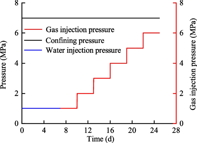
Schematic diagram of step loading

4.5 Test results
The curve of the water volume injected into the bentonite with time is shown in Fig. 14.

Variation curve of water volume injected into bentonite with time
It can be seen from Fig. 14 that the volume of water injected into the sample increased sharply with time at the initial stage, it tended to be stable after about 5 days. The bentonite shifted from unsaturated permeability to saturated permeability. According to Darcy's law, the permeability of the water injection stage was 1.31 × 10⁻²⁰ m2.
The confining pressure was set to be 7.0 MPa, and the injection pressures were 1.0 MPa, 2.0 MPa, 3.0 MPa, 4.0 MPa, 5.0 MPa, and 6.0 MPa. The permeation test obtained variation curves of at the outlet and pressure at the bentonite, as shown in Fig. 15.

Variation curve of pressure with time at both ends of bentonite under confining pressure of 7.0 MPa
As can be seen from Fig. 15, (1) In the injection stages of Pup = 1.0 MPa and Pup = 2.0 MPa, the pressure at the inlet end decreased linearly, the pressure at the outlet end increased erratically, and the pressure at the outlet increases slightly., because the bentonite was in an almost saturated state at the initial stage, where the capillary pressure inside the soil was high. On the other hand, when the gas injection pressure was low, the gas was dissolved in the water, no significant gas flux occurred, and no water outflow was observed at the outlet end. (2) In the injection stages of Pup = 3.0 MPa, Pup = 4.0 MPa and Pup = 5.0 MPa, the pressures at the inlet end and at the outlet end both varied linearly, and the pressure at the outlet increases faster. This variation is due to the fact that as the gas injection pressure increases, the pore space expands, and the gas flow path becomes wider, resulting in a more stable gas flow. No outflow of water was observed at the outlet end. (3) During the gas injection phase at Pup = 6.0 MPa, the pressure at the inlet end dropped abruptly, and the pressure at the outlet end increased abruptly after a few minutes. The range of the GDS pump to detect the outlet pressure was 1.0 MPa, so when the pressure was close to 1.0 MPa at the outlet side, the valve at the outlet side needed to be opened, and the pressure dropped sharply to 0 MPa. Then the outlet valve was closed again, and the pressure increased sharply. This increase indicated that a gas breakthrough occurred and a connected crack was generated within the bentonite. In addition, a mixture of bubbles interspersed with water was observed to be ejected, and the gas flow was very fast and turbulent. Many studies (Galle 2000; Harrington and Horseman 2005; Birgersson et al. 2008; Xu et al. 2015) have also reached a similar conclusion. When the gas pressure exceeds the sum of the tensile strength of the soil and the minimum principal stress, a continuous seepage path will be formed within the bentonite, and the gas breakthrough will occur.
The permeability and increasing rate of outlet pressure of the bentonite at different gas injection pressures are shown in Table 3 and Fig. 16.

Variation curves of permeability and increasing rate of outlet pressure with gas injection pressure
Combining Table 3 and Fig. 16, it can be seen that: As the gas injection pressure increased, the permeability and increasing rate of outlet pressure increased. When the gas injection pressure increased from 1.0 to 5.0 MPa, the increasing rate of outlet pressure increased from 1.8 × 10⁻⁴ to 1.84 × 10⁻³ MPa/h. Correspondingly, the permeability increased from 4.05 × 10⁻²¹ to 6.22 × 10⁻²¹ m2. When the gas injection pressure increased to 6.0 MPa, the permeability increased sharply to 6.57 × 10⁻¹⁹ m2, and the increasing rate of outlet pressure sharply increased to 3.94 MPa/h.
With the increase of gas injection pressure, the permeability and increasing rate of outlet pressure increased. According to the Griffith crack theory, the condition for the crack to stop spreading is that the decrease in strain energy is balanced by the increase in surface energy. Thus when the injection pressure was increased, the surface energy of the cracks within the bentonite rose and began to diffuse until a new equilibrium was reached. Whereas gas transport was mainly controlled by pore dilatancy effects, with slow expansion of cracks within the bentonite, forming a larger network of gas transport channels and exhibiting higher permeability and increased outlet pressure.
4.6 Comparison of experimental results with numerical simulation results
The permeability obtained from the numerical simulation in §3.2 was compared with the permeability obtained in the experiment, as shown in Table 4 and Fig. 17.

Comparison curves between the calculated values of permeability and the experimental value
Combining Table 4 and Fig. 17, it can be seen that: (1) when the gas injection pressure was between 1.0 MPa and 5.0 MPa, the permeability obtained by the experiment was not much different from the permeability obtained by numerical calculation, and the error was less than 10%. (2) When the gas injection pressure was 6.0 MPa, the permeability values obtained by experiment and simulation were quite different. (3) The permeability obtained by numerical simulation was slightly larger than that obtained by experiment under the same injection pressure. There are two possible reasons. On the one hand, the creep effect of the confining pressure over time may compact the pores in the permeation test, while the creep effect of the confining pressure was not considered in the numerical calculation. On the other hand, there is a certain capillary resistance in the permeability test when the gas migrates in the soil, but this part of the effect is less affected. However, the influence of two-phase flow on gas migration was not considered in the numerical calculation process. In summary, the permeability obtained from soil deformation and damage is not much different from the experimental results. The gas injection pressure (gas breakthrough pressure) at which the connected seepage path is formed is the same as that obtained from the experiment, which verifies the applicability and rationality of the model.
5 Conclusions
A coupled fluid-mechanical interaction model considering bentonite damage was developed in this paper. The numerical simulation of the bentonite stress field and seepage field was realized by the joint MATLAB and COMSOL secondary development, and the evolution law of pore path in bentonite under a flexible boundary was explored. The rationality and applicability of the model are verified by comparing the numerically calculated gas breakthrough pressure and permeability with the experimental values. From the above study, the following conclusions were drawn.
-
(1)
For the problem of bentonite stress and seepage fields, the controlling equations in the form of cylindrical coordinates were established, including the equilibrium equation considering the effect of effective stress and pore pressure on bentonite, geometric equation, physical equation, conservation of mass and momentum equation.
-
(2)
Tensile failure obeyed the Galileo criterion and shear failure obeyed the Coulomb-Mohr criterion. On this basis, damage variables were defined considering both tensile and shear damage modes. The elastic modulus after damage was described using damage variables, and the sudden increase coefficient of permeability was also introduced to describe the effect of damage variables on the permeability of bentonite.
-
(3)
According to the requirements of engineering in which the bentonite is located, the condition of the solution of bentonite stress field and seepage field were given. The controlling equations were combined with the condition of the solution to obtain the multi-physical field coupling model.
-
(4)
The pore expansion and permeability distribution pictures of bentonite at different gas injection pressures were obtained using a joint MATLAB and COMSOL secondary development. The gas breakthrough pressure determined from the damage area and the gas breakthrough pressure obtained from the permeability test were both 6.0 MPa. The permeability obtained by the experiment was not much different from the permeability obtained by numerical calculation, and the error was less than 10%, verifying the applicability and rationality of the proposed model.
Availability of data and materials
The data used in the manuscript is from experiment. You can contact Jingna Guo (guojingna@cuit.edu.cn) if you want learn more about our work.
References
Alonso J, Navarro V, Calvo B (2012) Flow path development in different CO2 storage reservoir scenarios: a critical state approach. Eng Geol 127(2):54–64. https://doi.org/10.1016/j.enggeo.2012.01.001
Arnedo D, Alonso EE, Olivella S (2014) Gas flow in anisotropic claystone: modelling triaxial experiments. Int J Numer Anal Methods Geomech 37(8):2239–2256. https://doi.org/10.1002/nag.2132
Birgersson M, Akesson M, Hokmark H (2008) Gas intrusion in saturated bentonite—a thermodynamic approach. Phys Chem Earth 33(10):248–251. https://doi.org/10.1016/j.pce.2008.10.039
Chilingar GV (1964) Relationship between porosity, permeability, and grain-size distribution of sands and sandstones. Dev Sedimentol 1(5):71–75. https://doi.org/10.1016/S0070-4571(08)70469-2
Cui LY, Ye WM, Wang Q, Chen YG, Chen B, Cui YJ (2022) Insights into gas migration in saturated GMZ bentonite using the RCP technique. Eng Geol 303:106646. https://doi.org/10.1016/j.enggeo.2022.106646
Galle C (2000) Gas breakthrough pressure in compacted Fo–Ca clay and interfacial gas overpressure in waste disposal context. Appl Clay Sci 17(2):85–97. https://doi.org/10.1016/S0169-1317(00)00007-7
Gerard P, Harrington J, Charlier R, Collin F (2014) Modelling of localised gas preferential pathways in claystone. Int J Rock Mech Min Sci 67(4):104–114. https://doi.org/10.1016/J.IJRMMS.2014.01.009
Gonzalez-Blanco L, Romero E, Jommi C, Li X, Sillen X (2016) Gas migration in a Cenozoic clay: experimental results and numerical modelling. Geomech Energy Environ 6(6):81–100. https://doi.org/10.1016/J.GETE.2016.04.002
Graham CC, Harrington JF, CussR J, Sellin P (2012) Gas migration experiments in bentonite: implications for numerical modelling. Mineral Mag 76(8):3279–3292. https://doi.org/10.1180/minmag.2012.076.8.41
Guo GL, Fall M (2021) Advances in modelling of hydro-mechanical processes in gas migration within saturated bentonite: a state-of-art review. Eng Geol. https://doi.org/10.1016/j.enggeo.2021.106123
Guo GL, Fall M (2018) Modelling of dilatancy-controlled gas flow in saturated bentonite with double porosity and double effective stress concepts. Eng Geol 243:253–271. https://doi.org/10.1016/j.enggeo.2018.07.002
Guo JN, Liu JF, Zhang Q, Cao SF, Chen ZQ (2022) Gas migration properties through saturated bentonite considering the interface effect. Geomech Geophys Geo-Energy Geo-Resour. https://doi.org/10.1007/s40948-022-00370-w
Gutierrez-Rodrigo V, Villar MV, Martin PL, Romero FJ, Barcala JM (2015) Gas-breakthrough pressure of FEBEX bentonite. Geol Soc Lond Spec Publ 415(1):47–57. https://doi.org/10.1144/SP415.4
Harrington JF, Horseman ST (2005) Gas migration in KBS-3 buffer bentonite. Sensitivity of test parameters to experimental boundary conditions
Harrington JF, Vaissiere RDL, Noy DJ, Cuss RJ, Talandier J (2012) Gas flow in Callovo-Oxfordian claystone (COx): results from laboratory and field-scale measurements. Mineral Mag 76(8):3303–3318. https://doi.org/10.1180/minmag.2012.076.8.43
Liu JF, Cao XL, Xu J, Yao QL, Ni HY (2020) A new method for threshold determination of gray image. Geomech Geophys Geo-Energy Geo-Resour. https://doi.org/10.1007/s40948-020-00198-2
Liu JF, Cao XL, Ni HY, Zhang K, Ma ZX, Ma LK, Pu H (2021) Numerical modeling of water and gas transport in compacted GMZ bentonite under constant volume condition. Geofluids 3:1–16. https://doi.org/10.1155/2021/4290426
Leupin OX, Smart NR, Zhang Z, Stefanoni M, Diomidis N (2021) Anaerobic corrosion of carbon steel in bentonite: an evolving interface. Corros Sci 187(32):109523. https://doi.org/10.1016/j.corsci.2021.109523
Ohno KI, Kitamura Y, Sukenaga S, Natsui S, Maeda T, Kunitomo K (2022) Gas permeability evaluation of granulated slag particles packed bed during softening and melting stage with Fanning’s equation. Tetsu-to-Hagane 108(10):703–712
Olivella S, Alonso EE (2008) Gas flow through clay barriers. Géotechnique 58(3):157–176. https://doi.org/10.1680/GEOT.2008.58.3.157
Ramesh S, Thyagaraj T (2022) Segmentation of X-ray tomography images of compacted soils. Geomech Geophys Geo-Energy Geo-Resour. https://doi.org/10.1007/s40948-021-00322-w
Tang CJ, Yao QL, Chen T, Shan CH, Li J (2022) Effects of water content on mechanical failure behaviors of coal samples. Geomech Geophys Geo-Energy Geo-Resour 8(3):87. https://doi.org/10.1007/s40948-022-00382-6
Tao J, Wu Y, Elsworth D, Li P, Hao Y (2019) Coupled thermo-hydro-mechanical-chemical modeling of permeability evolution in a CO2 -circulated geothermal reservoir. Geofluids. https://doi.org/10.1155/2019/5210730
Tawara Y, Hazart A, Mori K, Tada K, Shimura T, Sato S, Yamamoto S, Asano H, Namiki K (2014) Extended two-phase flow model with mechanical capability to simulate gas migration in bentonite. Geol Soc Lond Spec Publ 400(1):545–562. https://doi.org/10.1144/SP400.7
Wang JH, Elsworth D, Wu Y, Liu JS, Zhu WC, Liu Y (2018) The influence of fracturing fluids on fracturing processes: a comparison between water, oil and SC-CO2. Rock Mech Rock Eng 51:299–313. https://doi.org/10.1007/s00603-017-1326-8
Xu L, Ye WM, Ye B, Chen B, Chen YG, Cui YJ (2015) Investigation on gas migration in saturated materials with low permeability. Eng Geol 197(10):94–102. https://doi.org/10.1016/j.enggeo.2015.08.019
Xu WJ, Shao H, Hesser J, Wang W, Schuster K, Kolditz O (2013) Coupled multiphase flow and elasto-plastic modelling of in-situ gas injection experiments in saturated claystone (Mont Terri Rock Laboratory). Eng Geol 157(2):55–68. https://doi.org/10.1016/j.enggeo.2013.02.005
Yang TH, Liu J, Zhu WC, Elsworth D, Tham LG, Tang C (2007) A coupled flow-stress-damage model for groundwater outbursts from an underlying aquifer into mining excavations. Int J Rock Mech Min Sci 44(1):87–97. https://doi.org/10.1016/j.ijrmms.2006.04.012
Ye WM, Xu L, Chen B, Chen YG, Ye B, Cui YJ (2014) An approach based on two-phase flow phenomenon for modeling gas migration in saturated compacted bentonite. Eng Geol 169(2):124–132. https://doi.org/10.1016/j.enggeo.2013.12.001
Zhang Q, Ma D, Liu JF, Wang JH, Li XB, Zhou ZL (2019) Numerical simulations of fracture propagation in jointed shale reservoirs under CO2 fracturing. Geofluids. https://doi.org/10.1155/2019/2624716
Zhang Q, Wang JH, Gao YF, Cao SF, Xie JL, Ma LK, Liu YM (2021) CO2-driven hydraulic fracturing trajectories across a preexisting fracture. Geofluids 2021:1–12. https://doi.org/10.1155/2021/5533945
Zhu WC, Tang CA (2002) Numerical simulation on shear fracture process of concrete using mesoscopic mechanical model. Constr Build Mater 16(8):453–463. https://doi.org/10.1016/S0950-0618(02)00096-X
Zhu WC, Tang CA (2004) Micromechanical model for simulating the fracture process of rock. Rock Mech Rock Eng 37(1):25–56. https://doi.org/10.1007/s00603-003-0014-z
Zhu WC, Wei CH, Li S, Wei J, Zhang MS (2013) Numerical modeling on destress blasting in coal seam for enhancing gas drainage. Int J Rock Mech Min SCi 59:179–190. https://doi.org/10.1016/j.ijrmms.2012.11.004
Funding
This work has been supported by the China Atomic Energy Authority (CAEA) through the Geological Disposal Program, the National Natural Science Foundation of China (52104100), and China Postdoctoral Science Foundation (2021M703503), and Scientific Research Project of Chengdu University of Information Technology (376667).
Author information
Authors and Affiliations
Contributions
JG: Methodology, Data curation, Writing—original draft. QZ: Methodology, Writing—review & editing. LC: Investigation. SC: Validation. JX: Resources, Data curation. QL: Investigation. ZC: Conceptualization, Supervision.
Corresponding authors
Ethics declarations
Competing interests
The authors declare no competing interests.
Ethics approval and consent to participate
Not applicable.
Consent to publish
Not applicable.
Additional information
Publisher's Note
Springer Nature remains neutral with regard to jurisdictional claims in published maps and institutional affiliations.
Rights and permissions
Open Access This article is licensed under a Creative Commons Attribution 4.0 International License, which permits use, sharing, adaptation, distribution and reproduction in any medium or format, as long as you give appropriate credit to the original author(s) and the source, provide a link to the Creative Commons licence, and indicate if changes were made. The images or other third party material in this article are included in the article's Creative Commons licence, unless indicated otherwise in a credit line to the material. If material is not included in the article's Creative Commons licence and your intended use is not permitted by statutory regulation or exceeds the permitted use, you will need to obtain permission directly from the copyright holder. To view a copy of this licence, visit http://creativecommons.org/licenses/by/4.0/.
About this article

Cite this article
Guo, J., Zhang, Q., Chen, L. et al. A coupled fluid-mechanical interaction model for controlled gas migration mechanism by dilatancy effect in saturated bentonite. Geomech. Geophys. Geo-energ. Geo-resour. 9, 119 (2023). https://doi.org/10.1007/s40948-023-00647-8
Received:
Accepted:
Published:
DOI: https://doi.org/10.1007/s40948-023-00647-8