Birational geometry of smooth families of varieties admitting good minimal models

Abstract

We study families of projective manifolds with good minimal models. After constructing a suitable moduli functor for polarized varieties with canonical singularities, we show that, if not birationally isotrivial, the base spaces of such families support subsheaves of log-pluridifferentials with positive Kodaira dimension. Consequently we prove that, over special base schemes, families of this type can only be birationally isotrivial and, as a result, confirm a conjecture of Kebekus and Kovács.

1 Introduction and main results

A conjecture of Shafarevich and Viehweg predicts that smooth projective families of manifolds with ample canonical bundle (canonically polarized) whose algebraic structure maximally varies have base spaces of log-general type. This conjecture was settled through the culmination of works of many people, including Parshin [41], Arakelov [1], Kovács [36], Viehweg–Zuo [54], Kebekus–Kovács [26, 27], Patakfalvi [42] and Campana–Păun [5, 6].

More recently, triggered by [53] and the result of Popa–Schnell [43], it has been speculated that far more general results should hold for a considerably larger category of projective manifolds; those with good minimal models. In other words there is a conjectural connection between (birational) variation in smooth projective family of non-uniruled manifolds and global geometric properties of their base. In this setting the most general conjecture is a generalization of a conjecture of Campana which we resolve in this paper.

Theorem 1.1

(Isotriviality over special base) Let U and V be smooth quasi-projective varieties. If V is special, then every smooth projective family $f_U:U\rightarrow V$ of varieties with good minimal models is birationally isotrivial.

In this article all schemes are over $\mathbb {C}$. Following [51] and Kawamata [24, pp. 5–6] we define $\textrm{Var}\hspace{0.55542pt}(f_U)$ by the transcendence degree of a minimal closed field of definition K for $f_U$. We note that K is the minimal (in terms of inclusion) algebraically closed field in the algebraic closure $\overline{\mathbb {C}(V)}$ of the function field $\mathbb {C}(V)$ for which there is a K-variety W such that $U\hspace{0.55542pt}{\times }_V\hspace{1.111pt}\textrm{Spec}\hspace{0.55542pt}( \overline{\mathbb {C}(V)} )$ is birationally equivalent to $W\hspace{0.55542pt}{\times }_{\textrm{Spec}\hspace{0.55542pt}(K)}\hspace{1.111pt}\textrm{Spec}\hspace{0.55542pt}(\overline{\mathbb {C}(V)})$ (see Definition 3.16). By birationally isotrivial we mean $\textrm{Var}\hspace{0.55542pt}(f_U)=0$. We recall that an n-dimensional smooth quasi-projective variety V is called special if, for $1\leqslant p\leqslant n$, every invertible subsheaf verifies the inequality , where (B, D) is any smooth compatification of V, cf. [4]. Varieties with zero Kodaira dimension [4, Theorem 5.1] and rationally connected manifolds are important examples of special varieties.

In [49, Section 5] it was shown that, thanks to Campana’s results on the orbifold $C_{n.m}$ conjecture, once Theorem 1.1 is established the following conjecture of Kebekus–Kovács [26, Conjecture 1.6] (formulated in this general form in [43]) follows as a consequence.

Theorem 1.2

(Resolution of Kebekus–Kovács Conjecture) Let $f_U:U\rightarrow V$ be a smooth projective family of manifolds with good minimal models. Then, either

• (1.2.1) $\kappa (V) = -\infty$ and $\textrm{Var}\hspace{0.55542pt}(f_U) < \dim V$, or

• (1.2.2) $\kappa (V)\geqslant 0$ and $\textrm{Var}\hspace{0.55542pt}(f_U)\leqslant \kappa (V)$.

When $\textrm{Var}\hspace{0.55542pt}(f_U)$ is maximal ($\textrm{Var}\hspace{0.55542pt}(f_U) = \dim V$), these conjectures are all equivalent to Viehweg’s original conjecture generalized to the setting of manifolds admitting good minimal models. The latter is a result of [43] combined with [5].

For canonically polarized fibers Theorem 1.1 was settled in [48]. A key component of the proof was the following celebrated result of [56] for the base space of a projective family $f_U:U \rightarrow V$ of canonically polarized manifolds:

$(*)$ There are $k\in \mathbb {N}$ and an invertible subsheaf such that .

Establishing $(*)$ in the more general context of projective manifolds with good minimal models has been an important goal in this topic. In its absence, a weaker result was established in [49] where it was shown that for projective families with good minimal models we have:

$(**)$ There are $k\in \mathbb {N}$, a pseudo-effective line bundle and a line bundle on B, with such that .

Clearly $(**)$ is equivalent to $(*)$ when variation is maximal, in which case the result is due to [43, 53] when the base is of dimension one. But, as it is shown in [49] and [43, Subsection 4.3], the discrepancy between $(*)$ and $(**)$ poses a major obstacle in proving Kebekus–Kovács Conjecture in its full generality. In this paper we close this gap and prove the following result.

Theorem 1.3

Let $f_U:U\rightarrow V$ be a smooth, projective and non-birationally isotrivial morphism of smooth quasi-projective varieties U and V with positive relative dimension. Let (B, D) be a smooth compactification of V. If the fibers of $f_U$ have good minimal models, then there exist $k \in \mathbb {N}$ and an invertible subsheaf such that .

The fundamental reason underlying the difference between the two results $(**)$ and Theorem 1.3 is that while the proof of the former makes no use of a suitable moduli space associated to a relative minimal model program for the family $f_U$, the improvement in the latter heavily depends on a well-behaved moduli functor that we construct in Sect. 3 for any projective family of manifolds with good minimal models.

Theorem 1.4

Let $f_U:U\rightarrow V$ be a smooth projective family of varieties admitting good minimal models. For every family resulting from a relative good minimal model program for $f_U$, after removing a closed subscheme of V, there is an ample line bundle on $U'$ and a moduli functor ${{\,\mathrm{\mathfrak {M}}\,}}^{[N]}$ such that

where h is a fixed Hilbert polynomial. Moreover, the functor ${{\,\mathrm{\mathfrak {M}}\,}}_h^{[N]}$ has a coarse moduli space $M_h^{[N]}$ and that $\textrm{Var}\hspace{0.55542pt}(f_{U})$ is equal to the dimension of the image of V under the associated moduli map.

The existence of a functor ${{\,\mathrm{\mathfrak {M}}\,}}^{[N]}$ as in Theorem 1.4, approximating enough properties of the well-known functor for canonically polarized manifolds [52] for a prescribed family $f_U$ was not known before (see Proposition 3.10 and Theorem 3.18 for more details), which explains the focus of [43, Subsection 4.3] and subsequently [49] on the application of abundance type results to tackle Kebekus–Kovács Conjecture. The key advantage that Theorem 1.4 offers is that instead of constructing at the base of $f:X \rightarrow B$ we do so at the level of a moduli stack; a smooth projective variety Z equipped with a generically finite morphism to $M_h^{[N]}$ and parametrizing a new family, now with maximal (birational) variation. But once variation is maximal, again $(*)$ and $(**)$ are equivalent and the pseudo-effective line bundle in $(**)$ can essentially be ignored.

Since there are no maps from B to Z, the next difficulty is then to lift this big line bundle on Z to a line bundle on B. We resolve this problem by showing that the construction of such invertible sheaves is in a sense functorial. More precisely we show that the Hodge theoretic constructions in [49], from which these line bundle arise, verify various functorial properties that are sufficiently robust for the construction of the line bundle in Theorem 1.3, using the one constructed at the level of moduli stacks. This forms the main content of Sect. 2.

1.1 Notes on previously known results

When dimensions of the base and fibers are equal to one, Viehweg’s hyperbolicity conjecture was proved by Parshin [41], in the compact case, and in general by Arakelov [1]. For higher dimensional fibers and assuming that $\dim \hspace{0.55542pt}(V)=1$, this conjecture was confirmed by Kovács [36], in the canonically polarized case, and by Viehweg and Zuo [53] in general. Over abelian varieties Viehweg’s conjecture was solved by Kovács [35]. When $\dim \hspace{0.55542pt}(V)=2$ or 3, it was resolved by Kebekus and Kovács, cf. [26, 27]. In the compact case it was settled by Patakfalvi [42]. In the canonically polarized case, and when $\dim \hspace{0.55542pt}(V)\leqslant 3$, Theorem 1.1 is due to Jabbusch and Kebekus [20]. Using $(**)$ Kebekus–Kovács conjecture is settled in [49] under the assumption that $\dim \hspace{0.55542pt}(V) \leqslant 5$. More recently Theorem 1.1 for fibers of general type has appeared in the work of Wei–Wu [57].

2 Functorial properties of subsheaves of extended variation of Hodge structures arising from sections of line bundles

Our aim in this section is to show that the Hodge theoretic constructions in [49] enjoy various functorial properties. These will play a crucial role in the proof of Theorems 1.3 and 1.1 in Sect. 4.

Notation 2.1

(Discriminant) For a morphism $f:X \rightarrow Y$ of quasi-projective varieties with connected fibers, by $D_f$ we denote the divisorial part of the discriminant locus $\textrm{disc}\hspace{0.55542pt}(f)$. We define $\Delta _f$ to be the maximal reduced divisor supported over $f^{-1}D_f$.

2.1 Geometric setup

Let $f:X\rightarrow Y$ be a morphism of smooth quasi-projective varieties with connected fibers and relative dimension n. Let be a line bundle on X. We will sometimes need the extra assumption that

(2.1.1)

for some proper surjective morphism $\mu :T\rightarrow X$ from a smooth quasi-projective variety T. For example, the assumption (2.1.1) is valid when , in which case T can be taken to be any desingularization of the cyclic cover associated to a prescribed global section of [2] (see also [38, Proposition 4.1.6]).

Now, let be a morphism of smooth quasi-projective varieties and set to be a strong desingularization¹ of $Y^+ \hspace{0.55542pt}{\times }_Y\hspace{0.55542pt}X$ with the resulting family . Next, we define . Assuming that (2.1.1) holds, let $T^+$ be any smooth quasi-projective variety with a birational surjective morphism to a strong desingularization of $(T \hspace{1.111pt}{\times }_X\hspace{0.55542pt}X^+)$ with induced maps and . By construction we have

Finally, we define the two compositions

We will assume that $\Delta _f,\Delta _h,\Delta _{f^+}$ and $\Delta _{h^+}$ have simple normal crossing support (see Notation 2.1).

2.2 Hodge theoretic setup

In the setting of Sect. 2.1, after removing subsets of ${{\,\textrm{codim}\,}}\geqslant 2$ from the base, we may assume that $D_f$ and $D_h$ also have simple normal crossing support.

Let be a logarithmic system of Hodge bundles underlying the Deligne canonical extension of $\textrm{R}^n h_* {\underline{\mathbb {C}}\;}|_{T\setminus \Delta _h}$ (with the fixed interval [0, 1)). For every $0 \leqslant p \leqslant n$, and after removing a closed subset of Y along $D_h$ of ${{\,\textrm{codim}\,}}_{\hspace{1.111pt}Y}\geqslant 2$, let

$$\begin{aligned} \bigl ( \Omega ^{\bullet }_T (\log \Delta _h) , F_{T, \bullet } \bigr ) \end{aligned}$$

be the filtered logarithmic de Rham complex with the decreasing locally free filtration $F_{T, \bullet }$, with locally free gradings, induced by the exact sequence

$$\begin{aligned} 0 \longrightarrow h^* \Omega ^1_Y(\log D_h) \longrightarrow \Omega ^1_T (\log \Delta _h) \longrightarrow \Omega ^1_{T/Y}(\log \Delta _h) \longrightarrow 0. \end{aligned}$$

(2.1.2)

Let $C^p_T$ denote the complex corresponding to $\Omega ^p_T(\log \Delta _h)$ defined by the short exact sequence

$$\begin{aligned} 0 \longrightarrow h^* \Omega ^1_Y(\log D_h) \hspace{1.111pt}{\otimes }\hspace{1.111pt}\Omega ^{p-1}_{T/Y}(\log \Delta _h) \longrightarrow \frac{\Omega ^p_T (\log \Delta _h)}{F^2_{T,p}} \longrightarrow \Omega ^p_{T/Y}(\log \Delta _h) \longrightarrow 0, \end{aligned}$$

given by quotienting out by $F^2_{T,p}$. Thanks to Steenbrink [47] and Katz–Oda [23] we know there is an isomorphism of systems of Hodge bundles

with the Higgs field of the system on the right defined by the long exact cohomology sequence associated to ${{\,\mathrm{\textbf{R}}\,}}h_* C^p_T$ (which is a distinguished triangle in the bounded derived category of coherent sheaves).

Definition 2.2

Let be an -module on a regular scheme Y. Then, a -valued system consists of an -module and a sheaf homomorphism that is Griffiths-transversal with respect to an -module splitting , i.e. .

In particular, when and $\tau$ is integrable, is the usual system of Hodge sheaves.

Following the general strategy of [56] as we have seen in [49] we can construct an $\Omega ^1_Y(\log D_f)$-valued system . Furthermore, if the assumption (2.1.1) holds, then there is a map of systems

For the reader’s convenience we briefly recall the construction of [49, Subsection 2.2]. First note that, similarly to the construction of $C^p_T$, we can construct $C^p_X$ and consider the twisted short exact sequence .

Proposition 2.3

In the above setting, over the flat locus of f and h, for every $0\leqslant p \leqslant \dim \hspace{0.55542pt}(X/Y)$, there is a filtered morphism

(2.3.1)

Consequently, there is a morphism of short exact sequences .

Proof

First, we note that the pullback of short exact sequence of locally free sheaves

$$\begin{aligned} 0 \longrightarrow f^* \Omega ^1_Y(\log D_f) \longrightarrow \Omega ^1_X(\log \Delta _f) \longrightarrow \Omega ^1_{X/Y} (\log \Delta _f) \longrightarrow 0 \end{aligned}$$

via $\mu$ is a subsequence of (2.1.2). Therefore, by the construction of the two filtrations $F_{X,p}$ and $F_{T,p}$, cf. [16, Example 5.16 (c)], we have a filtered morphism

$$\begin{aligned} \mu ^* \bigl ( \Omega _X^p (\log \Delta _f) , F^j_{X,p} \bigr ) \rightarrow \bigl ( \Omega ^p_T (\log \Delta _h) , F^j_{T,p}\bigr ) . \end{aligned}$$

(2.3.2)

In particular, for $j=1,2$, we have

$$\begin{aligned} \mu ^* F^j_{X,p} \rightarrow F^j_{T,p} \end{aligned}$$

(2.3.3)

with the following commutative diagram:

(2.3.4)

Now, consider the commutative diagram

(2.3.5)

By the nine lemma, the diagram (2.3.5) induces

$$\begin{aligned} 0 \longrightarrow F^1_{X,p} / F^2_{X,p} \longrightarrow F^0_{X,p} / F^2_{X,p} \longrightarrow \Omega ^p_{X/Y} (\log \Delta _f) \longrightarrow 0, \end{aligned}$$

which we have denoted by $C^p_X$. By combining (2.3.4) and (2.3.3) and the functoriality of the nine lemma (in the abelian category of coherent sheaves), after pulling back (2.3.5) by $\mu$ we find the morphism

$$\begin{aligned} \mu ^* C^p_X \rightarrow C^p_T. \end{aligned}$$

(2.3.6)

Furthermore, by the assumption (2.1.1) we have the natural injection . This implies that there is a filtered injection

which, together with (2.3.2), establishes (2.3.1). Moreover, after twisting (2.3.5) by , again by the nine lemma (and its functoriality) we have

The proposition now follows from the composition of this latter morphism with (2.3.6).$\square$

Now, let be the system defined by

with each given by the connecting maps in the cohomology sequence associated to . By applying ${{\,\mathrm{\textbf{R}}\,}}\mu _*$ to the map in Proposition 2.3 we have

Using the (derived) projection formula and the adjunction map we thus get

and consequently the morphism

(2.3.7)

Proposition 2.4

(cf. [49, Subsection 2.2]) The morphism (2.3.7) induces the commutative diagram

where i is the natural inclusion map. The vertical maps on the left define by $\Phi = \bigoplus \Phi _i$. Furthermore, $\Phi _0$ is injective.

We can replicate this construction for . That is, assuming that $D_{f^+}$ and $D_{h^+}$ have simple normal crossing support and after removing a closed subscheme of $Y^+$ along $D_{f^+}$ of (if necessary), we can define two systems , whose graded pieces are given by

Similarly we can also define a morphism of systems on $Y^+$.

2.3 Functoriality. I

In the setting of Sect. 2.1, let and be the strong resolution defining $g'$ as the composition $\sigma \hspace{1.111pt}{\circ }\hspace{1.111pt}\pi$:

Lemma 2.5

There is a natural morphism

$$\begin{aligned} g^* {{\,\mathrm{\textbf{R}}\,}}f_* C^p_X \rightarrow {{\,\mathrm{\textbf{R}}\,}}f_*^+ \bigl ( (g')^* C^p_X\bigr ). \end{aligned}$$

Moreover, for any line bundle on X, we similarly have a morphism

Proof

By (derived) projection formula, and the fact that $C^p_X$ is locally free, we have

Together with the natural map (adjunction) we thus find

$$\begin{aligned} \sigma ^* C^p_X \rightarrow {{\,\mathrm{\textbf{R}}\,}}\pi _* \bigl ( (g')^* C^p_X \bigr ) . \end{aligned}$$

(2.5.1)

By applying ${{\,\mathrm{\textbf{R}}\,}}f'_*$ to (2.5.1) we then get

$$\begin{aligned} {{\,\mathrm{\textbf{R}}\,}}f_*' \bigl ( \sigma ^* C^p_X \bigr ) \rightarrow {{\,\mathrm{\textbf{R}}\,}}f_*^+ \bigl ( (g')^* C^p_X \bigr ). \end{aligned}$$

On the other hand, by (derived) base change, and flatness of g, we have ${{\,\mathrm{\textbf{R}}\,}}f'_* (\sigma ^*C^p_X)\cong g^* ( {{\,\mathrm{\textbf{R}}\,}}f_* C^p_X )$.

The second assertion in the proposition follows from an identical argument.$\square$

Assumption 2.6

From now on we will make the extra assumption that the morphism g is flat.

Proposition 2.7

With the assumption (2.1.1), in the setting of Sect. 2.2, there is a commutative diagram of morphisms of systems

which is an isomorphism over $Y^+\hspace{0.55542pt}{\setminus }\hspace{1.111pt}D_{f^+}$ for the vertical map on the left. Furthermore, the vertical map on the right is an injection over $Y^+$.

Proof

This is a direct consequence of base change and the functoriality of the construction of the systems involved. To see this, we note that there is a commutative diagram

so that, after applying ${{\,\mathrm{\textbf{R}}\,}}h^+_*$, by the projection formula we have

On the other hand, by Lemma 2.5 we have

By combining these two last diagrams we thus find

Existence of the map , and its compatibility with , now follows from the associated long exact cohomology sequences and flatness of g:

Furthermore, the assumption that g is flat implies that is an isomorphism over $Y^+ \hspace{0.55542pt}{\setminus }\hspace{1.111pt}D_{f^+}$.

Now, let $T'$ be a strong desingularization of $( X^+ \hspace{0.55542pt}{\times }_X T )$ such that there is a surjective birational map . Set to be the induced family and let be the Hodge bundle for the canonical extension of the VHS underlying $h'$. Then, again by base change, we know that there is a morphism

(2.7.1)

which is an isomorphism over $Y^+\hspace{0.55542pt}{\setminus }\hspace{1.111pt}D_{h'}$. The injectivity of (2.7.1) across $D_{h'}$ follows from the definition (or functoriality) of canonical extensions.

On the other hand, thanks to Deligne [10] and Esnault–Viehweg [13, Lemma 1.5], we know that ${{\,\mathrm{\textbf{R}}\,}}\sigma _* \Omega ^p_{T^+/Y^+} (\log \Delta _{h^+}) \cong \Omega ^p_{T'/Y^+}(\log \Delta _{h'})$ (see [54, 4.1.2] for the proof in the relative form). Therefore, which induces the required injection.$\square$

In the setting of Proposition 2.7, let and be, respectively, the image of and under $\Phi$ and $\Phi ^+$. In particular, for each i, we have

Due to the birational nature of the problems considered in this article, in application, we will be able to delete codimenison two subschemes of Y whose preimage under g are also of . Therefore, as g is flat, we may assume that the torsion free system is locally free. On the other hand, after replacing by its reflexive hull, we may also assume that is reflexive.

Assumption 2.8

The torsion free system is locally free and is reflexive.

By Proposition 2.7 we have a commutative diagram of systems

(2.8.1)

with all maps being injective over $Y^+$. Furthermore, the morphism

is an isomorphism over the $Y^+\hspace{0.55542pt}{\setminus }\hspace{1.111pt}D_{f^+}$.

We end this subsection with the following lemmas, which will be useful for application in Sect. 4. We will be working in the context of the following setup.

Set-up 2.9

Let $f:X\rightarrow B$ and $f_Z:X_Z \rightarrow Z$ be flat projective morphism with connected fibers of dimension n. Let and be two surjective flat morphisms. Assume that $\gamma$ is finite. All varieties are assumed to be smooth. Set $X^+_Z$ and $X'$ to be a strong desingularization of the normalization of $X\hspace{0.55542pt}{\times }_Z\hspace{1.111pt}Z^+$ and $X\hspace{0.55542pt}{\times }_B\hspace{1.111pt}Z^+$, respectively, with the naturally induced surjective morphisms , $g' :X^+_Z \rightarrow X_Z$, and . Assume that there is a birational map with $\pi ':{\widetilde{X}} \rightarrow X'$ and $\pi ^+:{\widetilde{X}}\rightarrow X^+$ removing its indeterminacy and so that $\Delta _{{\widetilde{f}}}$ is snc, where ${\widetilde{f}}:{\widetilde{X}}\rightarrow Z^+$ is the induced morphism. By construction we have and .

Given a line bundle on Z, define . Furthermore, set

Assuming that , let be a surjective morphism from a smooth quasi-projective variety $T^+$ associated to $s^+$, that is . Assume further that $\Delta _h$ is snc, where . Denote a strong desingularization of ${\widetilde{X}} \hspace{1.111pt}{\times }_{X^+}\hspace{0.55542pt}T^+$ by ${\widetilde{T}}$. Set ${\widetilde{\sigma }}:{\widetilde{T}} \rightarrow {\widetilde{X}}$ to be the induced morphism and assume that $\Delta _{{\widetilde{h}}}$ is snc, where , all fitting in the commutative diagram:

Set . Define . The natural inclusion (after raising the power to m) identifies a global section ${\overline{s}}$ of , determined by $s^+$. In particular the induced map factors through . Using the notations in Sect. 2.2, this implies that

commutes.

Furthermore, the inclusion is an equality over ${\widetilde{X}} \backslash \textrm{Exc}\hspace{0.55542pt}(\pi ')$. Thus, since is invertible and $X'$ is smooth, the section induces such that

$$\begin{aligned} (\pi ')^* s'|_{{\widetilde{X}}\backslash \textrm{Exc}\hspace{0.55542pt}(\pi ')} = {\overline{s}}|_{{\widetilde{X}} \backslash \textrm{Exc}\hspace{0.55542pt}(\pi ')} . \end{aligned}$$

(2.9.1)

Let ${\widehat{\sigma }}:{\widehat{T}}\rightarrow {\widetilde{X}}$ denote cyclic covering associated to $(\pi ')^*s'$. Using (2.9.1) and the construction of such coverings [38, pp. 243–244], ${\widehat{T}}$ and ${\widetilde{T}}$ are generically isomorphic. As such, after replacing ${\widehat{T}}$ by a higher birational model, we may assume that ${\widehat{T}}$ is smooth and ${\widehat{\sigma }}$ factors through ${\widetilde{\sigma }}:{\widetilde{T}} \rightarrow {\widetilde{X}}$ via a generically finite (in fact birational) morphism $\rho :{\widehat{T}} \rightarrow {\widetilde{T}}$. Let $\eta :{\widehat{T}} \rightarrow T^+$ and ${\widehat{h}}:{\widehat{T}}\rightarrow Z^+$ denote the naturally induced maps.

With the above construction we observe that, over the complement of $\textrm{Exc}\hspace{0.55542pt}(\pi ')$, the two injections and coincide, implying that:

Observation 2.10

The two naturally defined injections

coincide over the complement of  $\textrm{Exc}\hspace{0.55542pt}(\pi ')$.

Following the constructions in Sect. 2.2, let and be the logarithmic systems associated to the short exact sequences and. In particular we have

Similarly, define and to be the logarithmic systems respectively associated to and .

Let and be the logarithmic system of Hodge bundles associated to the canonical extension of the $\mathbb {C}$-VHS of weight n underlying the smooth loci of $h^+$ and ${\widehat{h}}$, and denote to be the image of the system associated to $C^p_{{\widetilde{T}}}$ in , induced naturally by $\rho ^*$.

Let and be the morphism of systems defined as in (2.3.7) and Proposition 2.4. Denote their images respectively by and . Furthermore, let and be morphisms of systems naturally defined by pullback morphisms $(\pi ^+)^*$ and $\eta ^*$. Similarly define and , with the image of the latter being denoted by . We summarize and further refine these constructions in the following lemma.

Lemma 2.11

In the setting of Set-up 2.9 we have:

• (2.11.1) There is a commutative diagram of systems

  

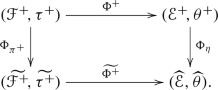
  In particular we have , where is the image of under $\Phi _{\eta }\hspace{1.111pt}{\circ }\hspace{1.111pt}\Phi ^+$.

• (2.11.2) .

• (2.11.3) There are natural morphisms . Denote the image of in by and that of in by . We have .

Proof

Item (2.11.1) simply follows from the constructions in Set-up 2.9 and the functorial properties of the morphisms in this diagram (remembering that as in (2.3.7) all are naturally defined by pullback maps). More precisely, setting , we note that the morphisms

are naturally defined by the pullback maps:

As such their composition, which we denote by $\Psi$, satisfies the following claim (Item (2.11.1)).

Claim 2.12

$\Psi$ factors through $\widetilde{\Phi ^+}$ via $\Phi _{\pi ^+}$.

Proof of Claim 2.12

By construction we know that factors through . After applying ${{\,\mathrm{\textbf{R}}\,}}{\widetilde{\tau }}_*$ we thus find the following commutative diagram of triangles in $D({\widehat{X}})$:

(2.12.1)

On the other hand, the diagram

naturally commutes. From (2.12.1) it thus follows that

(2.12.2)

After applying ${{\,\mathrm{\textbf{R}}\,}}\pi ^+_*$ to (2.12.2) we then get

The claim follows from applying ${{\,\mathrm{\textbf{R}}\,}}f^+_*$ to this latter commutative diagram. $\blacksquare$

Items (2.11.2) and (2.11.3) similarly follow from the constructions in Set-up 2.9.

$\square$

Lemma 2.13

In the situation of Set-up 2.9 and Lemma 2.11 we have .

Proof

This is a direct consequence of the constructions in (2.9) and Lemma 2.11. That is, we consider the auxiliary system associated to , where and denote its image under the natural map

by .

Claim 2.14

We have and .

Proof of Claim 2.14

By constructions in Set-up 2.9 and using the inclusion , ${\overline{\Phi }}$ factors as

which establishes the desired inclusions.

For the equality , note that by Observation 2.10 the maps

commute. Therefore, the images of and in coincide. $\blacksquare$

Now, by Lemma 2.11 we have and . On the other hand, by Claim 2.14 we have

Therefore, . $\square$

The next lemma helps with identifying a certain subsystem of (as in Set-up 2.9) which will be constructed in Proposition 2.17 (see also [57, Theorem 3.5.1]).

Lemma 2.15

Given as in Set-up 2.9, there is Higgs subsheaf with the following properties.

(2.15.1):

is injective. Denote the image of under $\Phi _{\eta }$ by .

(2.15.2):

and thus, as , we have .

Proof

Let and be the two flat logarithmic connections underlying and , respectively, and the morphism of holomorphically flat bundles corresponding to $\Phi _{\eta }$. Set $Z_0\subseteq Z^+$ to be the maximal open subset over which both and are polarized ${\mathbb {C}}$-VHSs defined by the smooth loci of $h^+$ and ${\widehat{h}}$, respectively. By Deligne [11, Proposition 1.13] over $Z_0$ both and are semisimple. Let be the smallest direct sum of simple summands that contains , remembering that $h^+_*\Omega ^n_{T^+/Z^+}(\log \Delta _{h^+})$ is the extension of the lowest piece of the Hodge filtration (and as such is contained in ).

Claim 2.16

is an injection.

Proof of Claim 2.16

Note that there is a natural injection

$$\begin{aligned} h^+_*\Omega ^n_{T^+/Z^+}(\log \Delta _{h^+}) \hookrightarrow {\widehat{h}}_*\Omega ^n_{{\widehat{T}}/Z^+} (\log \Delta _{{\widehat{h}}}) \end{aligned}$$

(which is an isomorphism as $\eta$ is birational) so that by the construction of $\Phi _{\eta }$ (or $\phi _{\eta }$) we have the commutative diagram

where is the image of ; again a semisimple flat bundle. Now, if is not injective, then identifies with a proper summand of . In particular $h^+_*\Omega ^n_{T^+/Z^+}(\log \Delta _{h^+})|_{Z^0}$ is contained in a smaller direct sum of simple summands of than those forming , contradicting the minimality assumption on the latter. $\blacksquare$

Now, according to the fundamental result of Jost–Zuo [22], over smooth quasi-projective varieties, there is an equivalence of categories between semisimple local systems and tame harmonic bundles. Therefore, underlies a tame harmonic bundle (with in particular a structure of a Higgs bundle) over $Z^0$ (see also Mochizuki [39]). Moreover, by the construction of , using the above equivalence of categories and the fact that is the canonical extension of a tame harmonic bundle over $Z^0$ [47, 40, Section 22.1], is a direct summand. Further, as a tame harmonic bundle, extends to a logarithmic Higgs bundle on $Z^+$ [40, Section 22.1] (after removing some subscheme of $Z^+$ of if necessary), whose eigenvalues of the associated residue map are contained in [0, 1). By uniqueness of the canonical extension (and its construction) it follows that is also a direct summand of .

On the other hand, from Claim 2.16, and again using the above equivalence of categories, it follows that is injective. As is torsion free, we find that must be injective, verifying Item (2.15.1).

For Item (2.15.2), by the construction of and , the bundle contains . On the other hand, we know that is a direct summand. Therefore, as is torsion free, the naturally defined map is indeed an inclusion. For the rest, note that by Lemma 2.11 the inclusion factors through and therefore by applying $\Phi _{\eta }$ to we find .$\square$

Proposition 2.17

In the situation of Set-up 2.9, assume further that $f_Z$ is semistable and that

for some $N\in \mathbb {N}$ and $D_Z\geqslant 0$. Then, we can find a $\gamma ^*\Omega ^1_B(\log D)$-valued subsystem

equipped with an isomorphism . Furthermore, over $Z^+\backslash D_{f^+}$, is also $(g^*\Omega ^1_Z)$-valued, i.e., we have

Proof

We first make the following observation.

Claim 2.18

(as defined in Set-up 2.9) is $(\gamma ^*\Omega ^1_B(\log D))$-valued.

Proof of Claim 2.18

Since $f_Z$ is semistable and g is flat, by [51, Section 3] we have . Therefore, we find , i.e.,

for some .

Let us first assume that . Consider the system on B defined by , where , with .

Subclaim 2.19

We have

Proof of Subclaim 2.19

Since f is smooth over $X\backslash D_f$ (and thus ) it suffices to show that the isomorphism

(2.19.1)

holds. On the other hand, by construction we have

After taking the determinant we therefore find

Moreover, by flat base change we have

After removing a subset of and taking the determinant we find the desired isomorphism in the subclaim. $\blacksquare$

Thus, according to Proposition 2.7 we have , which establishes the claim.

Now, assume that . As $\gamma$ is finite, it suffices to establish the claim over $B\backslash D_f$. Therefore, we may assume that $f'$ and f are smooth. With there is a natural injection from which it follows that . This implies that

Using the construction in Sect. 2.2 it then follows that there is an injection , proving the claim. $\blacksquare$

Now, set

so that is a subsystem of both and . In particular we have

As the subsystem is a Higgs subsheaf of , by Lemma 2.15, there is a $\Phi _{\eta }$-induced isomorphic subsystem of which is a Higgs subsheaf of . In particular we have . Moreover, since and thus is $(\gamma ^*\Omega ^1_B(\log D))$-valued, so is .

Furthermore, according to Proposition 2.7 we have the isomorphism of systems

Let be the subsystem of induced by via this isomorphism. Clearly the isomorphism implies that is $(g^*\Omega ^1_{Z\backslash D_f})$-valued.$\square$

2.4 Functoriality. II: descent of kernels

For the purpose of application later on in Sect. 4, we need to further refine our understanding of the properties of the systems constructed in Sect. 2.3, when g is induced by a flattening of a proper morphism, cf. [45]. To this end, we consider the following situation.

Let $f:V\rightarrow W$ be a projective morphism of smooth quasi-projective varieties with connected fibers of positive dimension. Let be a desingularization of a flattening of f, with the associated birational morphisms and , so that, by construction, every $f'$-exceptional divisor is $\pi$-exceptional.

Definition 2.20

(Codimension one flattening) In the above setting, let be the complement of the center of $\pi$. We call the induced flat morphism a codimension one flattening of f.

Notation 2.21

In the rest of this article we denote the reflexivization of the determinant sheaf by $\det \hspace{0.55542pt}(\hspace{1.111pt}{\cdot }\hspace{1.111pt})$.

We will be working in the setting of Set-up 2.9.

Notation 2.22

In the setting of Proposition 2.17 define and.

Proposition 2.23

(Descent of kernels of subsystems of VHS) In the setting of Sect. 2.9, assume that the varieties are projective and that the maps exist after removing closed subsets of Z and B of ${{\,\textrm{codim}\,}}\geqslant 2$. If is a codimension one flattening of a proper morphism with connected fibers, then, for every i, there is a pseudo-effective line bundle on Z such that

(2.23.1)

for some $a_i \in \mathbb {N}$.

Proof

After replacing Y and $Y^+$ by Z and $Z^+$ in Proposition 2.7, let be the image of . Set . We first consider the case where g is assumed to be proper. Again, as g is flat, pre-image of subsets of Y of ${{\,\textrm{codim}\,}}_{\hspace{1.111pt}Y} \geqslant 2$ are of and therefore we may assume that is locally free. From Diagram 2.8.1 (and Proposition 2.7) it follows that there is an injection

which is an isomorphism over $Z^+\hspace{0.55542pt}{\setminus }\hspace{1.111pt}D_{f_Z^+}$. Therefore, is g-effective and that , for a general point $z\in Z$. Thanks to properness and flatness of g, from the latter isomorphism it follows that

Therefore is trivial over Z. Consequently there is a line bundle on Z satisfying the isomorphism (2.23.1).

On the other hand, thanks to weak seminegativity of kernels of Higgs fields underlying polarized VHS of geometric origin [58] (see [49, Section 3] for further explanation and references), is pseudo-effective. Therefore so is , cf. [3].

For the case where g is not proper, we repeat the same argument for the flattening of g (from which g arises), after removing the non-flat locus from the base.$\square$

Next, we recall the trick of Kovács and Viehweg–Zuo involving iterated Kodaira–Spencer maps, which we adapt to our setting.

Lemma 2.24

In the setting of Proposition 2.17, assume that . Then, up to a suitable power, there is an integer $m>0$ for which $\theta ^+$ induces an injection

(2.24.1)

for some $k\in \mathbb {N}$ and where is a pseudo-effective line bundle on Z. Furthermore, over $Z^+\backslash D_{f^+}$ the injection (2.24.1) factors through the inclusion

Proof

By Proposition 2.17 we have so that . Noting that (again by Proposition 2.17) we have , for any non-negative integer i, we consider the image under the morphism

Let so that there is an injection

where (as in Notation 2.22).

Claim 2.25

$m\geqslant 1$.

Proof of Claim 2.25

If the map is zero, then is anti-pseudo-effective [58]. But this contradicts the inequality . $\blacksquare$

Now, from the inclusion of the systems we know that (Proposition 2.17). Therefore, there is an injection

Consequently, we find the desired injection (2.24.1). The isomorphism involving the pseudo-effective line bundle follows from Proposition 2.23.

The last assertion is the direct consequence of the fact that by Proposition 2.17 we have .$\square$

3 A bounded moduli functor for polarized schemes

In this section we will construct a moduli functor that is especially tailored to the study of projective families of good minimal models with canonical singularities (see [32, 34] for background on the minimal model program and the relevant classes of singularities). Let us first recall a few standard notations and definitions. In this section all schemes are assumed to be separated and of finite type (see [52, p. 12]).

Let X be a normal scheme and $K_X$ its canonical divisor. By $\omega _X$ we denote the divisorial sheaf . For a morphism of normal schemes $f:X\rightarrow B$, assuming that $K_B$ is Cartier, we set , where . Given a coherent sheaf on X and any $m\in \mathbb {N}$, we define to be the m-th reflexive power of .

Definition 3.1

(Relative semi-ampleness) Given a proper morphism of $f:X\rightarrow B$ of schemes and a line bundle on X, we say is semi-ample over B, or f-semi-ample, if for some $m\in \mathbb {N}$ the line bundle is globally generated over B, that is the natural map is surjective.

We note that from the definition it follows that for f-semi-ample we have a naturally induced morphism

(3.1.1)

over B, with a B-isomorphism . In particular is globally generated, for every $b\in B$. Moreover, we say is f-ample, if is f-semi-ample and the morphism (3.1.1) is an embedding over B (see for example [38, Section 1.7] for more details).

Notation 3.2

(Pullback and base change) For every morphism , we denote the fiber product $X\hspace{1.111pt}{\times }_B\hspace{0.55542pt}B'$ by $X_{B'}$, with the natural projections and . Furthermore, for a coherent sheaf on X, we define .

We begin by recalling Viehweg’s moduli functor ${{\,\mathrm{\mathfrak {M}}\,}}$ for polarized schemes [52, Section 1.1]. The objects of this functor are isomorphism classes of projective polarized schemes (Y, L), with L being ample. We write $(Y,L)\in \textrm{Ob}\hspace{0.55542pt}({{\,\mathrm{\mathfrak {M}}\,}})$. The morphism ${{\,\mathrm{\mathfrak {M}}\,}}:\mathfrak {Sch}_{\mathbb {C}} \rightarrow \mathfrak {Sets}$ is defined by

for any base scheme B. Here, the equivalence relation $\sim$ is given by

Definition 3.3

( [17, Definition 2.2]) Let ${\mathfrak {F}} \subset {\mathfrak {M}}$ be a submoduli functor. We say ${\mathfrak {F}}$ is open, if for every the set is open in B and . The submoduli functor ${\mathfrak {F}}\subset {\mathfrak {M}}$ is locally closed, if for every , there is a locally closed subscheme $j:B^u \hookrightarrow B$ such that for every morphism $\phi :T\rightarrow B$ we have: if and only if there is a factorization

We note that by definition ${\mathfrak {F}} \subset {{\,\mathrm{\mathfrak {M}}\,}}$ is open, if and only if it is locally closed and $B^u$ is open.

Definition 3.4

( [52, Definition 1.15 (1)]) Given a moduli functor of polarized schemes ${\mathfrak {F}}$, by ${\mathfrak {F}}_h$ we denote the submoduli functor whose objects (Y, L) have h as their Hilbert polynomial with respect to L. We say a submoduli functor ${\mathfrak {F}}_h \subset {\mathfrak {M}}_h$ is bounded, if there is $a_0\in \mathbb {N}$ such that, for every $(Y,L) \in \textrm{Ob}\hspace{0.55542pt}({\mathfrak {F}}_h)$ and any $a\geqslant a_0$, the line bundle $L^a$ is very ample and $H^i(Y, L^a)=0$, for all $i>0$.

For a positive integer N, we now consider a new submoduli functor ${{\,\mathrm{\mathfrak {M}}\,}}^{[N]}\subset {{\,\mathrm{\mathfrak {M}}\,}}$, whose objects (Y, L) verify the following additional properties:

• (3.4.1) Y has only canonical singularities.

• (3.4.2) $\omega _Y^{[N]}$ is invertible and semi-ample (N is not necessarily the minimum such integer).

• (3.4.3) For all $a\geqslant 1$, the line bundle $L^a$ is very ample and $H^i(Y,L^a)=0$, for all $i>0$.

Remark 3.5

Condition (3.4.3) means that ${{\,\mathrm{\mathfrak {M}}\,}}_h^{[N]}$ is bounded by construction (see Definition 3.4).

We note that, with fibers of $(f:X\,{\rightarrow }\, B) \in {\mathfrak {M}}(B)$ being normal, if B is nonsingular, then X is also normal. The following observation of Kollár shows that over nonsingular base schemes, for such morphisms a reflexive power N of $\omega _{X/B}$ is invertible. Therefore, over regular base schemes, the formation of $\omega _{X/B}^{[N]}$ commutes with pullbacks [17, Lemma 2.6]. We will see in Sect. 3.1 that this property is crucial for ${\mathfrak {M}}^{[N]}_h$ to be well-behaved.

Claim 3.6

(cf. [8, Lection 6]) Let $f:X\rightarrow B$ be a flat projective morphism of varieties, with B being smooth. If $X_b$ has only canonical singularities with invertible $\omega _{X_b}^{[N]}$, then $\omega _X^{[N]}$ and thus $\omega ^{[N]}_{X/B}$ are invertible near $X_b$. Moreover, $\omega _{X/B}^{[N]}$ is flat over a neighborhood of b.

Proof of Claim 3.6

For every $x\in X_b$, let $\rho _x:U'_x \rightarrow U_x$ be the local lift of the index-one covering of $(X_b, x)$ over an open subset $V_x\subseteq B$ [8, Corollary 6.15] so that $\omega _{(U'_x)_b}$ is invertible. By construction $(U'_x)_b$ has only canonical and therefore rational singularities [34, Corollary 5.25]. As rational singularities degenerate into rational singularities [12], $U'_x$ has rational singularities and the induced family $f\hspace{0.55542pt}{\circ }\hspace{1.111pt}\rho _x:U'_x \rightarrow V_x$ has Cohen–Macaulay fibers (after restricting to a smaller subset, if necessary). Using base change through $b\rightarrow V_x$ we thus find that $(\omega _{U'_x/V_x})_{b}$ is invertible [9, 3.6.1]. Therefore, so is $\omega _{U'_x/V_x}$. Since V is regular, it follows that $\omega _{U'_x}$ is also invertible. Consequently $N\hspace{1.111pt}{\cdot }\hspace{1.111pt}K_{U_x}$ is Cartier, as required. Furthermore, $\omega _{U'_x/V_x}$ is flat over $V_x$, and thus so is $(\rho _x)_*\hspace{1.111pt}\omega _{U'_x/V_x}$. On the other hand, by construction, $\omega ^{[N]}_{U_x/V_x}$ is a direct summand of $(\rho _x)_*\hspace{1.111pt}\omega _{U'_X/V_x}$, cf. [14, Corollary 3.11]. Therefore, $\omega ^{[N]}_{Ux/V_x}$ is flat over $V_x$. $\square$

3.1 The parametrizing space of ${{\,\mathrm{\mathfrak {M}}\,}}_h^{[N]}$

Our aim is now to show that the functor ${{\,\mathrm{\mathfrak {M}}\,}}^{[N]}_h$ has an algebraic coarse moduli space. The next proposition is our first step towards this goal. For the definition of a separated functor of polarized schemes we refer to [52, Definition 1.15 (2)].

Notation 3.7

For any $d\in \mathbb {N}$, by ${{\,\textrm{Hilb}\,}}^d_h$ we denote the Hilbert scheme of projective subschemes of ${\mathbb {P}}^{\,d}$ with Hilbert polynomial h.

Proposition 3.8

The subfunctor ${{\,\mathrm{\mathfrak {M}}\,}}_h^{[N]}\subset {{\,\mathrm{\mathfrak {M}}\,}}_h$ is open (thus locally closed) and separated.

Proof

We first show that ${{\,\mathrm{\mathfrak {M}}\,}}^{[N]}$ is open (Definition 3.3). This can be done by establishing the openness of each of Properties (3.4.1)–(3.4.3) in the following order, assuming that the special fiber $X_b$ is an object of ${{\,\mathrm{\mathfrak {M}}\,}}^{[N]}$. Using base change, we may assume that B is nonsingular (which implies that X is assumed to be normal).

Very ampleness: Using the vanishing from [38, Theorems 1.2.17 and 1.7.8], in the very ample case, it follows that the morphism arising from the canonical map is an immersion along $X_b$ and thus an immersion over an open neighborhood of b. In particular each is very ample over this neighborhood.

Degeneration of index and singularities: By Claim 3.6 we know that $\omega ^{[N]}_{X/B}$ is invertible near $X_b$. We also know that nearby fibers are all normal (in fact rational [12]). Therefore, by base change, we find that, for every $b'$ near b, we have , showing that the nearby fibers are of index N too.

Now, the fact that X has only canonical singularities near $X_b$ follows from [25], when $\dim \hspace{0.55542pt}(B)=1$. When $\dim \hspace{0.55542pt}(B)=2$, we consider the normalization of a curve passing through b and use inversion of adjunction, cf. [34, Section 5.4]. For higher dimensions we argue similarly using induction on $\dim \hspace{0.55542pt}(B)$.

Global generation: To show that semi-ampleness of the canonical divisor is open (openness of (3.4.2)), we note that $\omega _{X/B}^{[N]}$ is invertible and flat over a neighborhood of b (Claim 3.6). Let $\nu$ be an integer for which $\omega _{X_b}^{[N]\hspace{1.111pt}{\cdot }\hspace{1.111pt}\nu }$ is globally generated. According to Takayama [50], the function $b' \mapsto h^0(X_{b'}, \omega _{X_b'}^{[N]\cdot \nu })$ is constant over the open neighborhood of b where each $X_{b'}$ has only canonical singularities. Therefore, by [16, Corollary 12.9], the natural map

$$\begin{aligned} f_*\hspace{1.111pt}\omega ^{[N]\cdot \nu }_{X/B} \hspace{1.111pt}{\otimes }\hspace{1.111pt}\mathbb {C}(b) \rightarrow H^0\bigl (X_b, \omega ^{[N]\cdot \nu }_{X_b}\bigr ) \end{aligned}$$

is an isomorphism in a neighborhood of b. On the other hand, the restriction map is surjective. Therefore, using Nakayama’s lemma, we find that the canonical map $f^* f_* \hspace{1.111pt}\omega ^{[N]\cdot \nu }_{X/B} \rightarrow \omega ^{[N]\cdot \nu }_{X/B}$ is surjective along $X_b$. It follows that this map is surjective over a neighborhood of b, i.e. $\omega _{X/B}^{[N]\cdot \nu }$ is globally generated over this neighborhood.

It remains to verify that ${{\,\mathrm{\mathfrak {M}}\,}}_h^{[N]}$ is separated. Let R be a discrete valuation ring (DVR for short) and K its field of fractions. Define $B=\textrm{Spec}\hspace{0.55542pt}(R)$ and consider two polarized families

(3.8.1)

that are isomorphic (as families of polarized schemes) over $\textrm{Spec}\hspace{0.55542pt}(K)$. Let us denote this isomorphism by $\sigma ^{\circ } :X_1^{\circ } \rightarrow X_2^{\circ }$, where $X_i^{\circ }$ denotes the restriction of the family $X_i$ to $\textrm{Spec}\hspace{0.55542pt}(K)$, and, for every $b\in B$, define , , with $X_{i,0}$ denoting the special fiber. Using the two properties in Item (3.4.3), for $i=1,2$, as was shown in the very-ampleness case, we find that the natural morphisms are embeddings over B and

Claim 3.9

In this context, using the morphism , we can find Cartier divisors

such that near the special fibers $X_{i,0}$ we have:

• (3.9.1) $D_i$ avoids the generic point of every fiber $X_{i,b}$,

• (3.9.2) $D_1|_{X_1^0} = (\sigma ^\circ )^* D_2$, and that,

• (3.9.3) for some integer m, $\bigl (X_{i,0}, \frac{1}{m} D_{i,0}\bigr )$ is log-canonical (lc for short), where.

Proof of Claim 3.9

By Item (3.4.3), and using the fact that the Hilbert polynomial is fixed in the family, we have , for some $d\in \mathbb {N}$. With ${{\,\mathrm{\mathfrak {M}}\,}}_h^{[N]}$ being bounded, we have

Since $\psi _i$ is embedding over B and is fiberwise isomorphic to ${\mathbb {P}}^{\,d}$ we have .

Furthermore, the isomorphism over $\textrm{Spec}\hspace{0.55542pt}(K)$ naturally induces the $(\textrm{Spec}\hspace{0.55542pt}K)$-isomorphism

and the resulting diagram

(3.9.1)

which commutes over $\textrm{Spec}\hspace{0.55542pt}(K)$. Now, using this construction, including the fact that $\psi _i$ is fiber-wise embedding, for a general member , we can ensure that is a divisor on $X_i$ that does not contain the generic point of $X_{i,0}$. Moreover, by the commutativity of (3.9.1) we have $(\sigma ^0)^* D_2 = D_1$. Finally, let m be sufficiently large so that $\bigl (X_{i,0}, \frac{1}{m} D_{i,0}\bigr )$ is lc. This finishes the proof of the claim. $\blacksquare$

Now, using Claim 3.6, by inversion of adjunction we find that $\bigl (X_i, \frac{1}{m}D_i + X_{i,0}\bigr )$ is lc and thus, by specialization, so is $\bigl (X_{i,b}, \frac{1}{m}D_{i,b}\bigr )$, for a general $b\in \textrm{Spec}\hspace{0.55542pt}(K)$, where . Also, as $D_i$ is fiber-wise very amply, using nefness of $K_{X_i/B}$ we find that $K_{X_i/B}+ \frac{1}{m} D_i$ is fiber-wise ample so that, for each i, $\bigl (f_i:\bigl (X_i, \frac{1}{m} D_i\bigr ) \,{\rightarrow }\, B\bigr )$ is a stable family of pairs, cf. [33, Definition-Theorem 4.7]. Now, thanks to the separatedness of functors of stable families of pairs [33, Theorem 4.1] over regular base schemes, the two families $\bigl (f_1:\bigl (X_1, \frac{1}{m}D_1\bigr ) \,{\rightarrow }\, B\bigr )$ and $\bigl (f_2:\bigl (X_2, \frac{1}{m} D_2\bigr ) \,{\rightarrow }\, B\bigr )$ are isomorphic over B (as families of pairs), near the special fiber. In particular we have

as required.$\square$

The following proposition is now a consequence of Proposition 3.8 and a collection of well-known results in the literature. For the definition and basic properties of algebraic spaces we refer to [37, Chapters 1, 2].

Proposition 3.10

The moduli functor ${{\,\mathrm{\mathfrak {M}}\,}}_h^{[N]}$ has an algebraic space of finite type $M_h^{[N]}$ as its coarse moduli.

Proof

Using Item (3.4.3) for every $(Y,L) \in \textrm{Ob}\hspace{0.55542pt}({{\,\mathrm{\mathfrak {M}}\,}}^{[N]}_h)$ we have $h^0(L)=d+1$, for some $d\in \mathbb {N}$. Set to be the universal object with

We note that by Proposition 3.8, ${\mathfrak {M}}_h$ is bounded and locally closed, with L being very ample for every $(Y,L) \in {\mathfrak {M}}^{[N]}$. Therefore, there is a subscheme such that restricts to the universal family for the associated Hilbert functor of embedded schemes in ${\mathfrak {M}}_h^{[N]}$

via cf. [52, Section 1.7]. Now, as $H^u$ is naturally equipped with the action of , following [52], we need to show that the quotient of $H^u$ by $\mathbb PG$ is a geometric categorical quotient (see [31, Definition 2.7] or [28, Definition 1.8] for the definition). Thanks to [31, Theorem 1.5], [28, Corollary 1.2] and [52, Section 7.2] it suffices to establish the following claim.

Claim 3.11

The action ${\overline{\sigma }}$ of  $\mathbb PG$ on $H^u$ is proper, that is the morphism

is proper. Consequently, the action of on $H^u$ is proper with finite stabilizers.

Proof of Claim 3.11

We follow the arguments of [52, Lemma 7.6]. We recall that by the valuative criterion [31, Lemma 2.4] it suffices to show that for every DVR R, with field of fractions K, $B= \textrm{Spec}\hspace{0.55542pt}(R)$, and any commutative diagram

(3.11.1)

there is an extension ${\overline{\delta }}:B \rightarrow \mathbb PG\hspace{1.111pt}{\times }\hspace{1.111pt}H$ such that ${\overline{\delta }}|_{\textrm{Spec}\hspace{0.55542pt}K}= \delta$ and $\tau = {\overline{\psi }}\hspace{1.111pt}{\circ }\hspace{1.111pt}{\overline{\delta }}$. To do so we consider the two families

defined by the pullback of the universal family via ${{\,\textrm{pr}\,}}_i{\circ }\hspace{1.111pt}\tau$. From (3.11.1) it follows that there is a commutative diagram

which gives a $\textrm{Spec}\hspace{0.55542pt}(K)$-isomorphism $\phi :X_1\rightarrow X_2$ and a sheaf isomorphism over $\textrm{Spec}\hspace{0.55542pt}(K)$ . As ${\mathfrak {M}}^{[N]}_h$ is separated, both extend to isomorphisms over B, that is we have an isomorphism ${\overline{\phi }}:X_1\rightarrow X_2$, extending $\phi$, and an isomorphism

(3.11.2)

for some line bundle on B. We note that, similar to the proof of Claim 3.9, we have natural B-isomorphisms

On the other hand, (3.11.2) naturally induces the B-isomorphism

The extension ${\overline{\delta }} = ({\overline{\delta }}_1, {\overline{\delta }}_2)$ of $\delta$ can now be defined by

and .

Now, for the second assertion of the claim, using properness of ${\overline{\psi }}$, as G is finite over $\mathbb PG$, the composition

is proper. In particular we have properness of the fiber over $\{x\}\hspace{1.111pt}{\times }\hspace{1.111pt}H^u$, which forms the stabilizer of x in G. Therefore, with G being affine, the stabilizer of x must be finite.$\square$

Remark 3.12

We note that Claim 3.11 means that for every polarized scheme $(Y,L) = {\mathfrak {M}}^{[N]}_h(\textrm{Spec}\hspace{0.55542pt}(\mathbb {C}))$ the group of polarized automorphisms $\textrm{Aut}\hspace{0.55542pt}(Y,L)$ is finite.

3.2 Connection to the minimal model program

As we will see later in Sect. 4, for a smooth family of projective manifolds with good minimal models, it is quite useful to have an associated birationally-parametrizing space.

Given two quasi-projective varieties U and V, with V being smooth, we say U is a family of good minimal models over V, if there is a projective morphism $f_{U}:U\rightarrow V$ with connected fibers and an integer $N\in {\mathbb {N}}$ such that, for every $v\in V$, $U_v$ has only canonical singularities and that the reflexive sheaf $\omega _{U/V}^{[N]}$ is invertible and $f_U$-semi-ample (Definition 3.1). We sometimes refer to $f_{U}$ as a relative good minimal model.

Theorem 3.13

(Theorem 1.4) Let $U''$ be a family of good minimal models over $V''$ via the flat projective morphism . There is a very ample line bundle on $U''$ (not unique) and a polynomial h such that .

Proof

We only need to check the existence of satisfying (3.4.3). Let be a very ample line bundle on $U''$. From the flatness assumption on $f''$ we know that is constant for all $v\in V''$. Therefore, by semicontinuity [16, Theorem 12.8], for a sufficiently large $a\in \mathbb {N}$, the line bundle restricted to each fiber verifies (3.4.3), for every $m\geqslant a$. That is, for , we have , for all $b\geqslant 1$ and $v\in V$.$\square$

Remark 3.14

Following the proof of Theorem 3.13, we note that if we replace the line bundle by , for any $m\geqslant 1$, the conclusions of the theorem are still valid.

Our next aim is to show that for a suitable choice of a invertible sheaf we can ensure that the dimension of subspaces of $M^{[N]}_h$ are closely related to the variation of families mapping to them (see Theorem 3.18 below).

Set-up 3.15

Let be a relative good minimal model. According to [24, Lemma 7.1] there are smooth quasi-projective varieties ${\overline{V}}$ and $V''$, a surjective morphism $\rho :{\overline{V}} \rightarrow V''$ and a surjective, generically finite morphism $\sigma :{\overline{V}}\rightarrow V$ with a projective morphism :

(3.15.1)

satisfying the following properties:

• (3.15.2) Over an open subset the morphism $\sigma$ is finite and étale.

• (3.15.3) We have

  

  with and being the natural projections.

• (3.15.4) For every $t \in {\overline{V}}{}^\circ$ the kernel of $(d_t\rho \hspace{1.111pt}{\circ }\hspace{1.111pt}d_t\sigma ^{-1})$ coincides with the kernel of the Kodaira–Spencer map for at $u= \sigma (t)$, where $d_t \rho$ and $d_t \sigma$ are the differentials of $\rho$ and $\sigma$.

Theorem-Definition 3.16

( [24, Lemma 7.1, Theorem 7.2]) For every family of good minimal models , the algebraic closure is the (unique) minimal closed field of definition for $f_{U'}$, that is $\textrm{Var}\hspace{0.55542pt}(f_{U'}) = \dim V''$.

We note that, as $\textrm{Var}\hspace{0.55542pt}(\hspace{1.111pt}{\cdot }\hspace{1.111pt})$ is a birational invariant, for any projective family $f_U:U\rightarrow V$ that is birational to a relative good minimal model $U'$ over V, we have $\textrm{Var}\hspace{0.55542pt}(f_U)= \dim \hspace{0.55542pt}(V'')$.

One can observe that [24, Lemma 7.1, Theorem 7.2] in particular implies that, for families of good minimal models, variation is measured at least generically (over the base) by the Kodaira–Spencer map. Of course this property fails in the absence of the good minimal model assumption (for example one can construct a smooth projective family of non-minimal varieties of general type with zero variation and generically injective Kodaira–Spencer map). For future reference, we emphasize and slightly extend this point in the following observation.

Observation 3.17

We will work in the the situation of Set-up 3.15.

(3.17.1):

For every smooth subvariety $T\subseteq \overline{V}{}^\circ$, with $\rho (T)$ being a closed point, the family $\overline{U}{}_T^\circ \rightarrow T$ is trivial. In particular, if $\textrm{Var}\hspace{0.55542pt}(f_{U'}) =0$, then $f_{U'}$ is generically (over V) isotrivial.

(3.17.2):

For every $T\subseteq \overline{V}{}^\circ$ as in Item (3.17.1) and line bundle on $U''$, the polarized family 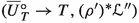is trivial.

To see this, we may assume that ${\overline{V}}{}^\circ = {\overline{V}}$. Set . By the assumption we have

$$\begin{aligned} {\overline{U}}_T \cong T \hspace{1.111pt}{\times }_{\mathbb {C}}\hspace{0.55542pt}F \end{aligned}$$

where (which shows Item (3.17.1)). Thus, over T, $\rho '$ coincides with the natural projection ${{\,\textrm{pr}\,}}_2:T\hspace{1.111pt}{\times }_{\mathbb {C}}\hspace{1.111pt}F\rightarrow F$. Clearly, is trivial.

Theorem 3.18

In the setting of Set-up 3.15, over an open subset $V_{\eta }$ of V there is a line bundle (not unique) such that , with the induced morphism $\mu _{V_{\eta }}:V_{\eta } \rightarrow M_h^{[N]}$ verifying the equality

$$\begin{aligned} \textrm{Var}\hspace{0.55542pt}(f_{U'}) = \dim \hspace{0.55542pt}( \textrm{Im}\hspace{0.55542pt}(\mu _{V_{\eta }}) ). \end{aligned}$$

(3.18.1)

In particular, any relative good minimal model of any smooth family $f_U:U\rightarrow V$ of projective varieties with good minimal model gives rise to a morphism of this form.

Proof

We start by considering Diagram 3.15.1. In Set-up 3.15 we may assume that ${\overline{V}}= {\overline{V}}{}^{\circ }$. Denote $U'\hspace{0.55542pt}{\times }_V\hspace{0.55542pt}{\overline{V}}$ by ${\overline{U}}$ and set ${\overline{f}}:{\overline{U}} \rightarrow {\overline{V}}$ to be the pullback family. Using Item (3.15.3), generically, the morphism $f''$ is a family of good minimal models (see also the global generation case in the proof of Proposition 3.8), that is after replacing V by an open subset $V_{\eta }$ we can assume that $f''$ is a relative good minimal model and flat. Let be a choice of line bundle as in the proof of Theorem 3.13 so that . We may assume that $\sigma$ is Galois, noting that if $\sigma$ is not Galois, we can replace it by its Galois closure and replace $\rho$ by the naturally induced map. Define .

Now, we define and consider the G-sheaf (see for example [18, Definition 4.2.5] for the definition). As $\sigma '$ is étale, the stabilizer of any point ${\overline{u}}\in {\overline{U}}$ is trivial (and thus so is its action on the fibers). Consequently, the above G-sheaf descends [18, Theorem 4.2.15]. That is, there is a line bundle on $U'_{V_{\eta }}$ such that

Therefore, we have

After replacing by , so that , we can ensure that the Hilbert polynomial of ${\overline{f}}$ with respect to is equal to the one for $f''$ with respect to . Let denote the induced moduli map.

Our aim is now to establish the equality (3.18.1). To this end, set W to be the image of $V_{\eta }$ under $\mu _{V_{\eta }}$.

Claim 3.19

$\dim W \geqslant \dim V''$.

Proof of Claim 3.19

Assume that instead $\dim W < \dim V''$. Let $T\subseteq V_{\eta }$ be a subscheme whose pre-image under $\sigma$ is generically finite over $V''$. This implies that $\dim T = \dim V''$ and that the variation of the induced family over T defined by pullback of $f''$ is maximal (see Item (3.15.4)). Now, by comparing the dimensions, we see that

$$\begin{aligned} \dim \hspace{0.55542pt}( \mu _{V_{\eta }}(T) ) < \dim T. \end{aligned}$$

But this contradicts the fact that the induced family over T has maximal variation. This can be seen as a consequence of Kollár’s result [29, Corollary 2.9] for families of varieties with non-negative Kodaira dimension. $\blacksquare$

Now, let $Z\subseteq V_{\eta }$ be a subscheme that is generically finite and dominantover W. By construction, the induced moduli map $\mu _{{\overline{V}}}:{\overline{V}}\rightarrow M_h^{[N]}$ associated to factors through $\mu _{V_{\eta }}$. Therefore, $\sigma ^{-1}(Z)$ is also generically finite over W.

Claim 3.20

$\sigma ^{-1}(Z)$ is generically finite over $V''$ and thus $\dim W\leqslant \dim V''$.

Proof of Claim 3.20

If $\rho |_{\sigma ^{-1}Z}:\sigma ^{-1}Z\rightarrow V''$ is not generically finite, then for each irreducible (positive dimensional) general fiber $T\subseteq \sigma ^{-1}(Z)$ mapping to a smooth closed point $v''$ Observation 3.17 (Item (3.17.2)) applies. Therefore, as the above choice of the polarization for the family defined by ${\overline{f}}$ is pullback of the one fixed for $f''$ via $\rho '$, the family is locally trivial as polarized schemes. Thus, by the construction of $\mu _{{\overline{V}}}$, the general fiber of $\sigma ^{-1}(Z) \rightarrow V''$ must be contracted by $\mu _{{\overline{V}}}$, contradicting the generic finiteness of $\mu _{{\overline{V}}}|_{\sigma ^{-1}(Z)}$. $\blacksquare$

The first half of the theorem now follows from Claims 3.19 and 3.20.

To see that every smooth projective family $f_U:U\rightarrow V$ of varieties admitting a good minimal model leads to a moduli morphism $\mu _{V_{\eta }}:V_{\eta }\rightarrow M_h^{[N]}$ as above, for some $N\in \mathbb {N}$, using the first half of the theorem, it suffices to know that f has a relative good minimal model . But this is guaranteed, for example by [15, 1.2, 1.4].$\square$

Notation 3.21

(Replacing $M^{[N]}_h$ by an étale covering) Let $M \rightarrow M^{[N]}_h$ be an étale covering, with M being a finite type scheme, cf. [37, Chapter 2] (see also [52, pp. 279–280]). Set $\mu '_{V_{\eta }}:V_{\eta }\rightarrow M$ to be the finite type morphism of schemes representing $\mu _{V_{\eta }}$ in this étale covering. Let $M^0\subseteq M$ be an affine subscheme containing the generic point of $\textrm{Im}\hspace{0.55542pt}(\mu '_{V_{\eta }})$. After replacing $V_{\eta }$ by we thus have a finite type morphism

of quasi-projective schemes. By abuse of notation, from now on we will denote $V^0_{\eta }$, $M^0$ by $V_{\eta }$ and $M^{[N]}_h$, respectively, that is $M^{[N]}_h$ is quasi-projective and is the induced moduli map.

Corollary 3.22

Let $f:X\rightarrow B$ be a smooth comapctification of a smooth projective family $f_U:U\rightarrow V$, whose fibres admit good minimal models. Then, depending on a choice of a relative good minimal model for $f_U$ there is a polarization as in Theorem 3.18 and, following the notation introduced in Notation 3.21, there is a rational moduli map $\mu _{V_{\eta }}:B \dashrightarrow {\overline{M}}_h^{[N]}$, where ${\overline{M}}_h^{[N]}$ is a compactification of $M_h^{[N]}$ by a projective scheme. Moreover, we have $\dim \hspace{0.55542pt}(\textrm{Im}\hspace{0.55542pt}(\mu _{V_{\eta }})) = \textrm{Var}\hspace{0.55542pt}(f_U)$.

4 Base spaces of families of manifolds with good minimal models

To prove Theorems 1.3 and 1.1 we will use the moduli functor in Theorem 3.18 to construct a new family $f_Z:X_Z \rightarrow Z$ out of the initial $f:X\rightarrow B$ over which the variation is maximal (Proposition 4.2 below). Serving as a key component of the proof of Theorem 1.3, the subsystems of canonical extensions of VHS in Sect. 2 will then be constructed for $f_Z$ and various families arising from it (see [54, Lemma 2.8]).

Notation 4.1

For a flat morphism $f:X\rightarrow Y$ of regular schemes, by $X^{(r)}$ we denote a strong desingularization of the r-th fiber product over Y

Noting that as $M_h^{[N]}$ is taken to be quasi-projective (Theorem 1.4 and Notation 3.21), as in Corollary 3.22 by ${\overline{M}}_h^{[N]}$ we denote its projective compactification. Since in what follows all our maps to $\overline{M}_h^{[N]}$ originate from reduced schemes, with no loss of generality we will assume that $\overline{M}_h^{[N]}$ is already reduced.

Proposition 4.2

In the setting of Corollary 3.22, assume that $\textrm{Var}\hspace{0.55542pt}(f_U)\ne 0$, $\textrm{Var}\hspace{0.55542pt}(f_U)\ne \dim (V)$ (see Definition 3.16) and set $n=\dim \hspace{0.55542pt}(X/B)$. After replacing B by a birational model, let ${\overline{\mu }}_{V_{\eta }}:B\rightarrow {\overline{M}}_h^{[N]}$ be a desingularization of $\mu _{V_{\eta }}$. Then, there are smooth projective varieties $Z^+$ and Z, a morphism and, after removing a subscheme of $Z^+$ of , a morphism that fit into the commutative diagram

(4.2.1)

verifying the following properties:

(4.2.2):

We have $\dim \hspace{0.55542pt}(B) = \dim \hspace{0.55542pt}(Z^+) > \dim \hspace{0.55542pt}(Z)$, where $\dim \hspace{0.55542pt}( Z) = \textrm{Var}\hspace{0.55542pt}(f_U)$. Moreover, there is a morphism $\overline{\mu }_{V_{\eta }}:B \rightarrow W$ with positive relative dimension, connected fibers and a generically finite map $\mu _Z :Z \rightarrow W$ such that the diagram

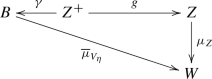
commutes.

(4.2.3):

The morphism is a codimension one flattening of a proper morphism (see Definition 2.20).

(4.2.4):

The two schemes $X_Z^+$ and $X_Z$ are regular and quasi-projective. The two morphisms $f_Z$ and $f_Z^+$ are projective with connected fibers. Moreover, $f_Z$ is semistable.

(4.2.5):

With $X'$ being a strong desingularization of $X \hspace{1.111pt}{\times }_B\hspace{0.55542pt}Z^+$, there is a birational map $\pi :X^+_Z \dashrightarrow X'$ over $Z^+$. The morphism is the naturally induced map.

(4.2.6):

For any $r\in \mathbb {N}$ there is an induced diagram involving similarly defined morphisms $f^{(r)}:X^{(r)} \rightarrow B$, $f_Z^{(r)}:X^{(r)}_Z \rightarrow Z$, ${f_Z^+}^{(r)} :{X_Z^+}^{(r)}\rightarrow Z^+$ and ${f'}^{(r)} :{X'}^{(r)} \rightarrow Z^+$ commuting with the ones in Diagram 4.2.1.

(4.2.7):

For any sufficiently large and divisible m, the line bundle defined by the reflexive hull of $\det \hspace{0.55542pt}(f_Z)_* \hspace{1.111pt}\omega ^{m}_{X_Z/Z}$ is big, implying that for a sufficiently large $N\in \mathbb {N}$ there is an ample line bundle , for some effective divisor $D_Z\geqslant D_{f_Z}$ on Z. Moreover, for sufficiently large integers m, there is $r\in \mathbb {N}$ such that , where

Proof

Let W be the image of $\overline{\mu }_{V_\eta }$. Using Stein factorization we replace W by a finite covering so that ${\overline{\mu }}_{V_{\eta }}$ has connected fibers. Take $Z\subset B$ to be a sufficiently general, smooth and complete-intersection subvariety such that is generically finite. By Corollary 3.22 we have $\dim Z =\textrm{Var}\hspace{0.55542pt}(f_U)$.

Define $Z^+$ to be a desingularization of the normalization of $B\hspace{1.111pt}{\times }_W \hspace{0.55542pt}Z$. Let be the resulting naturally defined map.

For Item (4.2.3), let be a flattening of g such that, after removing a subscheme of $Z^+$ of , the induced map is a codimension one flattening. We now replace Z by $Z'$.

As for Item (4.2.4), take $X_Z$ to be a strong desingularization of the pullback of $f:X\rightarrow B$ via the morphism $Z\rightarrow B$. Let ${\widehat{Z}}\rightarrow Z$ be a cyclic, flat morphism associated to a semistable reduction ${\widehat{f}}_Z:Z_{{\widehat{Z}}}\rightarrow {\widehat{Z}}$ in codimension one for $f_Z$. Again, after removing a subset of Z of (and therefore of $Z^+$ as g is flat), we replace $f_Z$ by ${\widehat{f}}_Z$. $X_{Z}^+$ is a desingularization of $X_Z \hspace{1.111pt}{\times }_Z\hspace{0.55542pt}Z^+$.

For Item (4.2.5), let $V_{\eta }$ be as in Theorem 3.18. Let $U'$ be a good minimal model over $V_{\eta }$ and set $Z_{\eta }$ to denote the restriction of Z to $V_{\eta }$. Define . As before $U'_{Z_{\eta }}$ and $U'_{Z_{\eta }^+}$ denote the pullback of $U'$ via $Z_{\eta }\rightarrow V_{\eta }$ and $Z_{\eta }^+\rightarrow V_{\eta }$, respectively. Next, define $(U'_{Z_{\eta }})^+$ to be the pullback of through $Z^+_{\eta }\rightarrow Z_{\eta }$. Summarizing this construction we have:

Claim 4.3

Up to a finite covering of $Z^+_{\eta }$, $(U'_{Z_{\eta }})^+$ is isomorphic to $U'_{Z_{\eta }^+}$ over $Z^+_{\eta }$.

Proof of Claim 4.3

This follows from the above construction, finiteness of the polarized automorphism groups in Remark 3.12 and the following fact, which is a consequence of representability of the isomorphism scheme for polarized projective varieties (cf. [27, Section 7] for the canonically polarized case).

Fact Assume that $X_i$ and Y are quasi-projective varieties, $i=1,2$. Let be two polarized flat projective families of varieties such that for every $y \in Y$ we have and . Then, there is a finite surjective morphism such that , extending the fiber-wise isomorphism. $\blacksquare$

Therefore, without loss of generality we may replace $Z^+$ by the finite covering defined in Claim 4.3. Consequently, we find a birational map over $Z^+$ as in Item (4.2.5).

Item (4.2.6) can be easily checked.

Item (4.2.7) is a deep result of Kawamata [24, Theorem 1.1] for smooth families of projective varieties with good minimal models, assuming that variation is maximal.

Moreover, given , we recall the natural inclusion

$$\begin{aligned} \bigl ( \det \hspace{0.55542pt}(f_Z)_*\hspace{1.111pt}\omega ^m_{X_Z/Z}\bigr )^m \subseteq \,\bigotimes ^{mr_m} \,(f_Z)_*\hspace{1.111pt}\omega ^m_{X_Z/Z} , \end{aligned}$$

(4.3.1)

where, using the semistability of $f_Z$, the right-hand side is isomorphic to

cf. [51, Section 3]. This implies that

$$\begin{aligned} h^0\bigl ( \omega _{X_Z^{(r)}/Z} \hspace{1.111pt}{\otimes }\hspace{1.111pt}\bigl (f_Z^{(r)}\bigr )^* \bigl (\det \hspace{0.55542pt}(f_Z)_*\hspace{1.111pt}\omega ^m_{X_Z/Z}\bigr )^{-1} \bigr )^m\ne \, 0. \end{aligned}$$

(Note that following the setting of the proposition we may ignore closed subset of .)

Now, after replacing the power m on the left-hand side of (4.3.1) by Nm, and using the definition of we find that

(4.3.2)

where r is now set as $Nmr_m$. As and $D_Z\geqslant D_{f_Z}$, we have

which together with (4.3.2) implies (4.2.8). $\square$

4.1 Proof of Theorem 1.3

Let $f:X\rightarrow B$ be a smooth compactification of $f_U$ such that, consistent with the rest of this paper, D in the setting of the theorem will be replaced by the notation $D_f$. When $\textrm{Var}\hspace{0.55542pt}(f_U) = \dim B$, the theorem is due to [55], in the canonically polarized case, and [43] in general (see also [49]). So assume that $\textrm{Var}\hspace{0.55542pt}(f_U) \ne \dim B$.

By Proposition 4.2 we know that $f:X\rightarrow B$ fits inside the diagram (4.2.1). For now let us identify f with its base change. After replacing X by $X^{(r)}$, for sufficiently large r (Item (4.2.6)), let be the line bundle on $X_Z$ defined in (4.2.7), namely

(4.3.3)

By Item (4.2.7) we know that . For the moment we will assume that $\gamma$ is finite (and therefore flat). As such, and using the birational map $\pi$, the constructions and conclusions of Lemmas 2.11, 2.15 and Proposition 2.17 are valid. As (see Set-up 2.9), by using the map (2.24.1), for some $k\in {\mathbb {N}}$, we have an injective morphism

As is big in Z and $\mu _Z$ is generically finite, we have . Let us denote the saturation of the image of

(4.3.4)

by . After deleting appropriate subscheme of B of ${{\,\textrm{codim}\,}}_B\geqslant 2$, using its Galois closure, we may also assume that is Galois. Set . It follows that the G-sheaf descends [18, Theorem 4.2.15], that is

(4.3.5)

for some line bundle on B. Therefore, the two line bundles in (4.3.5) have the same Kodaira dimension, cf. [19, Lemma 10.3] and we have , as required.

Since, after removing a ${{\,\textrm{codim}\,}}_B\geqslant 2$-subscheme of B, the morphism $\gamma$ is finite, and as our ultimate goal is birational, following the above argument, we may assume with no loss of generality that $\gamma$ is indeed finite. This is not difficult to check (using Stein factorization) and we leave the details to the reader.

Finally, we note that the above argument shows that we may assume with no loss of generality that $f:X\rightarrow B$ is identified with the required finite base change in Proposition 4.2. This finishes the proof of Theorem 1.3.

4.2 Proof of Theorem 1.1

To prove Theorem 1.1 we need a refinement of the statement of Theorem 1.3 in the sense of Theorem 4.7 . As one would expect, the proof of this refinement is inextricably intertwined with that of Theorem 1.3 itself. We note that in the canonically polarized case this refinement is due to Jabbusch–Kebekus [21]. The notion of orbifolds, as developed by Campana, is the key ingredient for realizing this improvement of Theorem 1.3. We refer to the original paper of Campana [4] for the basic definitions and further background. For the reader’s convenience, a brief summary of all required notions in this theory has been included in the appendix.

Set-up 4.4

We will be working in the setting of Proposition 4.2. The line bundles and are the ones defined in (4.3.4) and (4.3.5). To lighten up the notations we will use ${\overline{\mu }}$ to denote ${\overline{\mu }}_{V_{\eta }}$. Let $D_f = D_f^v + D_f^h$ be the decomposition of D into vertical and horizontal components with respect to ${\overline{\mu }}$. Let $W^0\subseteq W$ be the maximal open subset over which ${\overline{\mu }}:(B, D_f)\rightarrow W$ is neat. By construction, over $W^0$ there is a natural map

(4.4.1)

(cf. [20, Section 5.B]). Set to be the saturation of the image of (4.4.1).

Proposition 4.5

Assume that $W^0=W$. Let be the line bundle in (4.3.5). There is an injection .

Proof

Let be the torsion free cokernel of . Since $\gamma$ is flat, we have the short exact sequence

with being torsion free in codimension one.

Claim 4.6

Let be the line bundle on $Z^+$ defined in (4.3.4). After removing a subset of $Z^+$ of if necessary, the injection

factors through .

Proof of Claim 4.6

First, we observe that by Lemma 2.24 we have

Furthermore, again by Lemma 2.24, over an open subset $Z^+_0 \subseteq Z^+$ (given by $Z^+\backslash D_{f^+}$) we have . Using the commutativity of the diagram

this in particular implies that over an open subset of W the line bundle injects into . This means that at least over an open subset of $Z^+$ the factorization in Claim 4.6 holds. In other words, the naturally induced map

has a nontrivial kernel. As is torsion free in codimension one, it follows that this map is zero in codimension one, implying the desired injection in Claim 4.6. $\blacksquare$

Now, we may assume with no loss of generality that the inclusion

is saturated and that $\gamma$ is Galois. By (4.3.5) we have . We may also assume that $|G|=1$ (as we may replace k by k|G|). Now, by applying $\gamma _*(\hspace{1.111pt}{\cdot }\hspace{1.111pt})^G$ to the injection in Claim 4.6 we find the injection in codimension one, which as is reflexive, extends to an injection over B.$\square$

Theorem 4.7

In the situation of Set-up 4.4, let ${\widetilde{\mu }}:({\widetilde{B}}, {\widetilde{D}})\rightarrow {\widetilde{W}}$ be a neat model for ${\overline{\mu }}:(B, D_f) \rightarrow W$, via birational morphisms $\alpha$ and $\pi$ (see Definition 5.3), and with the orbifold base $({\widetilde{W}}, \Delta _{{\widetilde{W}}})$ (Definition 5.15). Let be the saturation of the image of

where $({\widetilde{D}})^\textrm{v}$ denotes the vertical component of ${\widetilde{D}}$ (with respect to ${\widetilde{\mu }}$). Then, there is a line bundle on ${\widetilde{B}}$, with , and equipped with an injection .

Proof

Let ${\widetilde{Z}}$ be a desingularization of the main component of ${\widetilde{B}} \hspace{1.111pt}{\times }_B \hspace{1.111pt}Z^+$, with the naturally induced maps ${\widetilde{\gamma }}:{\widetilde{Z}}\rightarrow {\widetilde{B}}$ and ${\widetilde{\pi }}:{\widetilde{Z}}\rightarrow Z^+$. Set . The proof is now the same as that of Proposition 4.5 after replacing ${\overline{\mu }}:(B,D_f)\rightarrow W$, and , by ${\widetilde{\mu }}:({\widetilde{B}}, {\widetilde{D}})\rightarrow {\widetilde{W}}$, ${\widetilde{\gamma }}:{\widetilde{Z}}\rightarrow {\widetilde{B}}$ and , respectively.$\square$

4.2.1 Generic descent to coarse space as an orbifold base; conclusion of the proof of Theorem 1.1

With Theorem 4.7 at hand, noting that , the proof of Theorem 1.1 is now identical to [48], for which [5] or [6] provides a vital ingredient (see also Claudon’s Bourbaki exposition [7]).

Aiming for a contradiction, we assume that $f_U$ is not isotrivial. Thanks to the already established results in the maximal variation case [5, 43, 55] we know $\textrm{Var}\hspace{0.55542pt}(f_U) \ne \dim \hspace{0.55542pt}(V)$. In particular the constructions of Proposition 4.2 and those of Sect. 4.1 apply. Furthermore, as specialness is a birational invariant for log-smooth pairs, we may replace $(B,D) \rightarrow W$ (with $D=D_f$) by its neat model $({\widetilde{B}}, {\widetilde{D}})\rightarrow {\widetilde{W}}$ as in Theorem 4.7. At this point [20, Corollary 5.8] applies, that is there is a line bundle in , for some $N\in \mathbb {N}$, with (see Definition 5.14 for the definition of ). It then follows that $\kappa ( {\widetilde{W}}, \Delta _{{\widetilde{W}}} ) = \dim {\widetilde{W}}$ [48, Theorem 5.2], which in turn implies that $({\widetilde{B}}, {\widetilde{D}})$ is not special, and thus neither is (B, D), contradicting our initial assumption.

Appendix: Background on orbifolds

In this appendix for the convenience of the reader we review some basic elements of Campana’s theory of orbifolds [4]. Most of the definitions in this appendix have been taken from [48].

Definition 5.1

A pair, or an orbifold pair, consists of a variety Y and a ${\mathbb {Q}}$-Weil divisor $D= \sum d_i D_i$, where $d_i \in [0,1]\cap {\mathbb {Q}}$ and each $D_i$ is prime. We say (Y, D) is snc, if Y is smooth and D has a simple normal crossing support.

Given a quasi-projective morphism $h:(Y,D) \rightarrow W$ with connected fibers and ${\mathbb {Q}}$-factorial W, there is a pair $(W, \Delta _W)$, referred to as the orbifold base or -base associated to h and D, see for example [20, Definition 5.3] or Definition 5.15.

Definition 5.2

We say $h:(Y,D) \rightarrow W$ as above is neat if

• (5.2.1) (Y, D) and the orbifold base $(W, \Delta _W)$ are snc, and

• (5.2.2) every h-exceptional divisor $P\subset Y$ (${{\,\textrm{codim}\,}}_{\hspace{1.111pt}W}(h(P)) \geqslant 2$) is contained in $\textrm{Supp}\hspace{0.55542pt}(D)$ as a reduced divisor.

Definition 5.3

(cf. [48, Definition 4.1]) Given any pair (Y, D) and a morphism $h:Y \rightarrow W$, a neat morphism ${\widetilde{h}}:({\widetilde{Y}}, D_{{\widetilde{Y}}}) \rightarrow {\widetilde{W}}$ is called a neat model for $h:(Y,D)\rightarrow W$ if

• (5.3.1) ${\widetilde{h}}:{\widetilde{Y}} \rightarrow {\widetilde{W}}$ is birationally equivalent to $h:Y\rightarrow W$, i.e., we have a commutative diagram

  

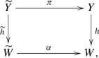
  where $\alpha , \pi$ are birational morphisms, and

• (5.3.2) $D_{{\widetilde{Y}}}$ is the sum of the total $\pi$-transform of D and all ${\widetilde{h}}$-exceptional divisors in ${\widetilde{Y}}$ (as reduced divisors).

Remark 5.4

For any (Y, D) and $h:Y\rightarrow W$ as in Definition 5.3 a neat model can be constructed (not uniquely), cf. [20, Section 10] or [48, Proposition 4.2]. The construction is originally due to Campana.

Notation 5.5

Given an snc pair (Y, D), for each $i \in {\mathbb {N}}$, by we refer to the i-th tensorial orbifold (or -)differential forms. See for example [48, Definition 2.8, Remark 2.11] or Remark 5.13.

Definition 5.6

Let $(X,D = \sum d_i D_i)$ be snc. When $d_i\ne 1$, let $a_i$ and $b_i$ be the positive integers for which the equality $1-{b_i}/{a_i}=d_i$ holds. For every i, we define the -multiplicity of the irreducible component $D_i$ of D by

Definition 5.7

Let (X, D) be a smooth pair, Y a smooth variety, and $\gamma :Y \rightarrow X$ a finite, flat, Galois cover with Galois group G such that if $m_D(D_i)={a_i}/{b_i}<\infty$, then every prime divisor in Y that appears in $\gamma ^*(D_i)$ has multiplicity exactly equal to $a_i$. We call $\gamma$ an adapted cover for the pair (X, D), if it additionally satisfies the following properties:

• (5.7.1) The branch locus is given by

  

  where H is a general member of a linear system |L| of a very ample divisor L in X.

• (5.7.2) $\gamma$ is totally branched over H.

• (5.7.3) $\gamma$ is not branched at the general point of $\textrm{Supp}\hspace{0.55542pt}(\lfloor D \rfloor )$.

Notation 5.8

Let $\gamma :Y\rightarrow X$ be an adapted cover of a smooth pair (X, D), where $D=\sum d_iD_i$, $d_i=1-{b_i}/{a_i}$ as in Definition 5.6. For every prime component $D_i$ of D with $m_D(D_i)\ne \infty$, let $\{D_{ij}\}_{j(i)}$ be the collection of prime divisors that appear in $\gamma ^{-1}(D_i)$. We define new divisors in Y by

Definition 5.9

Given an snc pair (X, D) with an adapted cover $\gamma :Y\rightarrow X$, define the -cotangent sheaf (or orbifold cotangent sheaf) $\Omega ^1_{(Y, \gamma , D)}$ to be the unique maximal locally-free subsheaf of $\Omega ^1_Y(\log D_{\gamma })$ for which the sequence

induced by the natural residue map, is exact.

Definition 5.10

Let (X, D) be snc, $D=\sum d_iD_i$, and $V_x$ an open neighbourhood of a given point $x\in X$ equipped with a coordinate system $z_1,\ldots ,z_n$ such that $\textrm{Supp}\hspace{0.55542pt}(D)\cap V_x=\{z_1 \cdots z_l=0\}$, for a positive integer $1\leqslant l\leqslant n$. For every $N\in \mathbb {N}^+$, define the sheaf of symmetric orbifold or -differential forms by the locally-free subsheaf of $\textrm{Sym}\hspace{0.55542pt}^N (\Omega ^1_X(\log (\ulcorner D \urcorner )))$ that is locally-generated, as an -module, by the elements

$$\begin{aligned} \frac{dz_1^{k_1}}{z_1^{\lfloor d_1\cdot k_1\rfloor }} \cdot \ldots \cdot \frac{dz_l^{k_l}}{z_l^{\lfloor d_l\cdot k_l \rfloor }} \cdot dz_{l+1}^{k_{l+1}} \hspace{1.111pt}{\cdot }\hspace{1.111pt}\ldots \hspace{1.111pt}{\cdot }\hspace{1.111pt}dz_n^{k_n}, \end{aligned}$$

where $\sum k_i =N$.

Remark 5.11

There is an alternative definition for the sheaf of -differential forms: Let $V_x$ be an open neighbourhood of $x\in X$ as in Definition 5.10 and take $\gamma :W \rightarrow V_x$ to be an adapted cover for $(V_x,D|_{V_x})$. Let $\sigma \in \Gamma (V_x,\textrm{Sym}\hspace{0.55542pt}^{N}(\Omega ^1_X(*\ulcorner D \urcorner )))$, that is $\sigma$ is a local rational section of $\textrm{Sym}\hspace{0.55542pt}^{N}(\Omega _X)$ with poles along $\ulcorner D \urcorner$. Then,

So that, in particular, $\gamma ^*(\sigma )$ has at worst logarithmic poles only along those prime divisors in W that dominate $(\lfloor D \rfloor \cap V_x)$, and is regular otherwise.

Explanation 5.12

Assume that is a local -differential form in the sense of Remark 5.11. It follows that

$$\begin{aligned} \sigma \in \Gamma \bigl (V_x,\textrm{Sym}\hspace{0.55542pt}^N\bigl (\Omega ^1_X\log (\ulcorner D \urcorner )\bigr )\bigr ). \end{aligned}$$

In particular we find that along the reduced component of D the equivalence between the two definitions trivially holds. So assume, without loss of generality, that $m_D(D_i)\ne \infty$, for all irreducible components $D_i$ of D. Furthermore let us assume, for simplicity, that

$$\begin{aligned} \sigma =f\hspace{1.111pt}{\cdot }\hspace{1.111pt}\frac{dz_1^{k_1}}{z_1^{e_1}}\hspace{1.111pt}{\cdot }\hspace{1.111pt}\ldots \hspace{1.111pt}{\cdot }\hspace{1.111pt}\frac{dz_l^{k_l}}{z_l^{e_l}}\cdot dz_{l+1}^{k_l+1}\hspace{1.111pt}{\cdot }\hspace{1.111pt}\ldots \hspace{1.111pt}{\cdot }\hspace{1.111pt}dz_n^{k_n} \in \Gamma \bigl (V_x,\textrm{Sym}\hspace{0.55542pt}^{N}\bigl (\Omega ^1_X \log \hspace{0.55542pt}(\ulcorner D \urcorner )\bigr )\bigr ) , \end{aligned}$$

where with no zeros along $D_i$’s, is the local explicit description of $\sigma$. Since $\gamma ^*(\sigma )\in \textrm{Sym}\hspace{0.55542pt}^N(\Omega ^1_{(W, \gamma , D|_{V_x})})$, the inequality

$$\begin{aligned} k_i\hspace{1.111pt}{\cdot }\hspace{1.111pt}(a_i-1)-a_i\hspace{1.111pt}{\cdot }\hspace{1.111pt}e_i \geqslant k_i(b_i-1) \end{aligned}$$

holds for $1\leqslant i\leqslant l$, where $d_i=1-b_i/a_i$, i.e.

$$\begin{aligned} e_i \leqslant k_i.d_i , \quad \text {for all}\;\; 1\leqslant i\leqslant l . \end{aligned}$$

In particular $\sigma$ is a symmetric -differential form on $V_x$ in the sense of Definition 5.10.

Remark 5.13

(Tensorial -differential forms) Similarlyy to the Definitions 5.10 and Remark 5.11, we can define the sheaf of tensorial -differential forms as the maximal subsheaf of $(\Omega ^1_X(\log (\ulcorner D \urcorner )))^{\otimes N}$ such that

Using the notations in Remark 5.11, pluri--differential forms are locally defined as follows:

$$\begin{aligned} \sigma \in \Gamma \Bigl (V_x,\bigl (\Omega ^1_X (\log D)\bigr )^{\otimes _{\mathscr {C}}N}\Bigr ) \iff \gamma ^{*}(\sigma )\in \Gamma \bigl (W, \Omega ^1_{(W, \gamma , D|_{V_x})} \bigr ) . \end{aligned}$$

(5.13.1)

Definition 5.14

Let (X, D) be an snc pair and a saturated coherent subsheaf of rank one. Define the -product of , to the order of m, to be the saturation of the image of inside and define the -Kodaira dimension of by

and when for all $m\in \mathbb {N^+}$, then, by convention, we define .

Definition 5.15

(Orbifold-base; the reduced case) Let (Y, D) be a pair and assume that D is reduced and Y is normal. Given a morphism $h:Y\rightarrow X$ with connected, positive-dimensional fibers and reduced, factorial X, let $\textrm{disc}\hspace{0.55542pt}(h) = \bigcup \Delta _i$ be the union of divisorial components of $\textrm{disc}\hspace{0.55542pt}(h)$. For every i, we have

$$\begin{aligned} h^*\Delta _i = \sum \, a_j \Delta '_{ij(i)} + E_i , \end{aligned}$$

where each $\Delta '_{ij}$ is prime, $a_i \in \mathbb {N}$ and $E_i$ is h-exceptional. For each i, if $\Delta '_{ij}\subseteq \textrm{Supp}\hspace{0.55542pt}(D)$, for every $\Delta '_{ij}$ in $h^{-1}(\Delta _i)$, set . Otherwise, let

Define the orbifold base (or -base) of $h:(Y,D)\rightarrow X$ by

References

Arakelov, S.Yu.: Families of algebraic curves with fixed degeneracies. Math. USSR-Izv. 5(6), 1277–1302 (1971)
Bloch, S., Gieseker, D.: The positivity of the Chern classes of an ample vector bundle. Invent. Math. 12, 112–117 (1971)
Boucksom, S., Demailly, J.-P., Păun, M., Peternell, T.: The pseudo-effective cone of a compact Kähler manifold and varieties of negative Kodaira dimension. J. Algebraic Geom. 22(2), 201–248 (2013)
Campana, F.: Orbifolds, special varieties and classification theory. Ann. Inst. Fourier (Grenoble) 54(3), 499–630 (2004)
Campana, F., Păun, M.: Positivity properties of the bundle of logarithmic tensors on compact Kähler manifolds. Compositio Math. 152(11), 2350–2370 (2016)
Campana, F., Păun, M.: Foliations with positive slopes and birational stability of orbifold cotangent bundles. Publ. Math. Inst. Hautes Études Sci. 129, 1–49 (2019)
Claudon, B.: Semi-positivité du cotangent logarithmique et conjecture de Shafarevich–Viehweg (d’aprés Campana, Păun, Taji, ...). Séminaire Bourbaki, vol. 2015/2016, no. 1105 (2015)
Clemens, H., Kollár, J., Mori, S.: Higher-Dimensional Complex Geometry. Astérisque, vol. 166. Société Mathématique de France, Paris (1989)
Conrad, B.: Grothendieck Duality and Base Change. Lecture Notes in Mathematics, vol. 1750. Springer, Berlin (2000)
Deligne, P.: Théorie de Hodge. II. Inst. Hautes Études Sci. Publ. Math. 40, 5–57 (1971)
Deligne, P.: Un théorème de finitude la monodromie. In: Howe, R. (ed.) Discrete Groups in Geometry and Analysis. Progress in Mathematics, vol. 67, pp. 1–19. Birkhäuser, Boston (1987)
Elkik, R.: Singularités rationnelles et déformations. Invent. Math. 47(2), 139–147 (1978)
Esnault, H., Viehweg, E.: Revêtements cycliques. In: Conte, A. (ed.) Algebraic Threefolds. Lecture Notes in Mathematics, vol. 947, pp. 241–250. Springer, Berlin (1982)
Esnault, H., Viehweg, E.: Lectures on Vanishing Theorems. DMV Seminar, vol. 20. Birkhäuser, Basel (1992)
Hacon, C.D., McKernan, J., Xu, C.: Boundedness of moduli of varieties of general type. J. Eur. Math. Soc. (JEMS) 20(4), 865–901 (2018)
Hartshorne, R.: Algebraic Geometry. Graduate Texts in Mathematics, vol. 52. Springer, New York (1977)
Hassett, B., Kovács, S.J.: Reflexive pull-backs and base extension. J. Algebraic Geom. 13(2), 233–247 (2004)
Huybrechts, D., Lehn, M.: The Geometry of Moduli Spaces of Sheaves. Cambridge Mathematical Library, 2nd edn. Cambridge University Press, Cambridge (2010)
Iitaka, S.: Algebraic Geometry. Graduate Texts in Mathematics, vol. 76. Springer, New York (1982)
Jabbusch, K., Kebekus, S.: Families over special base manifolds and a conjecture of Campana. Math. Z. 269(3–4), 847–878 (2011)
Jabbusch, K., Kebekus, S.: Positive sheaves of differentials coming from coarse moduli spaces. Ann. Inst. Fourier (Grenoble) 61(6), 2277–2290 (2012)
Jost, J., Zuo, K.: Harmonic maps of infinite energy and rigidity results for representations of fundamental groups of quasiprojective varieties. J. Differential Geom. 47(3), 469–503 (1997)
Katz, N.M., Oda, T.: On the differentiation of the de Rham cohomology classes with respect to parameters. J. Math. Kyoto Univ. 1, 199–213 (1968)
Kawamata, Y.: Minimal models and the Kodaira dimension of algebraic fiber spaces. J. Reine Angew. Math. 363, 1–46 (1985)
Kawamata, Y.: Deformations of canonical singularities. J. Amer. Math. Soc. 12(1), 85–92 (1999)
Kebekus, S., Kovács, S.J.: Families of canonically polarized varieties over surfaces. Invent. Math. 172(3), 657–682 (2008)
Kebekus, S., Kovács, S.J.: The structure of surfaces and threefolds mapping to the moduli stack of canonically polarized varieties. Duke Math. J. 155(1), 1–33 (2010)
Keel, S., Mori, S.: Quotients by groupoids. Ann. Math. 145(1), 193–213 (1997)
Kollár, J.: Subadditivity of the Kodaira dimension: fibers of general type. In: Oda, T. (ed.) Algebraic Geometry. Advanced Studies in Pure Mathematics, vol. 10, pp. 361–398. North-Holland, Amsterdam (1987)
Kollár, J.: Projectivity of complete moduli. J. Differential Geom. 32(1), 235–268 (1990)
Kollár, J.: Quotient spaces modulo algebraic groups. Ann. Math. 145(1), 33–79 (1997)
Kollár, J.: Singularities of the Minimal Model Program. In: Bertoin, J. (ed.) Cambridge Tracts in Mathematics, vol. 200. Cambridge University Press, Cambridge (2013)
Kollár, J.: Available online at author’s webpage: https://web.math.princeton.edu/~kollar/book/modbook20170720-hyper.pdf
Kollár, J., Mori, S.: Birational Geometry of Algebraic Varieties. Cambridge Tracts in Mathematics, vol. 134. Cambridge University Press, Cambridge (1998)
Kovács, S.J.: Families over a base with a birationally nef tangent bundle. Math. Ann. 308(2), 347–359 (1997)
Kovács, S.J.: Logarithmic vanishing theorems and Arakelov–Parshin boundedness for singular varieties. Compositio Math. 131(3), 291–317 (2002)
Knutson, D.: Algebraic Spaces. Lecture Notes in Mathematics, vol. 203. Springer, Berlin (1971)
Lazarsfeld, R.: Positivity in Algebraic Geometry. Vol. I. Ergebnisse der Mathematik und ihrer Grenzgebiete, vol. 48. Springer, Berlin (2004)
Mochizuki, T.: Kobayashi-Hitchin correspondence for tame harmonic bundles and an application. Astérisque, vol. 309. Société Mathématique de France, Paris (2006)
Mochizuki, T.: Asymptotic Behaviour of Tame Harmonic Bundles and an Application to Pure Twistor \(D\)-Modules. Vol. II. Memoirs of the American Mathematical Society, vol. 185(870). American Mathematical Society, Providence (2007)
Parshin, A.N.: Algebraic curves over function fields. I. Math. USSR-Izv. 2(5), 1145–1170 (1968)
Patakfalvi, Zs.: Viehweg’s hyperbolicity conjecture is true over compact bases. Adv. Math. 229(3), 1640–1642 (2012)
Popa, M., Schnell, C.: Viehweg’s hyperbolicity conjecture for families with maximal variation. Invent. Math. 208(3), 677–713 (2017)
Popa, M., Taji, B., Wu, L.: Brody hyperbolicity of base spaces of certain families of varieties. Algebra Number Theory 13(9), 2205–2242 (2019)
Raynaud, M., Gruson, L.: Critères de platitude et de projectivité. Techniques de “platification’’ d’un module. Invent. Math. 13, 1–89 (1971)
Siu, Y.-T.: Invariance of plurigenera. Invent. Math. 134(3), 661–673 (1998)
Steenbrink, J.: Limits of Hodge structures. Invent. Math. 31(3), 229–257 (1975/76)
Taji, B.: The isotriviality of smooth families of canonically polarized manifolds over a special quasi-projective base. Compositio Math. 152(7), 1421–1434 (2016)
Taji, B.: On the Kodaira dimension of base spaces of families of manifolds. J. Pure Appl. Algebra 225(11), 106729 (2021)
Takayama, S.: On the invariance and the lower semi-continuity of plurigenera of algebraic varieties. J. Algebraic Geom. 16(6), 1–18 (2007)
Viehweg, E.: Weak positivity and the additivity of the Kodaira dimension for certain fibre spaces. In: Iitaka, S. (ed.) Algebraic Varieties and Analytic Varieties. Advanced Studies in Pure Mathematics, vol. 1, pp. 329–353. North-Holland, Amsterdam (1983)
Viehweg, E.: Quasi-Projective Moduli for Polarized Manifolds. Ergebnisse der Mathematik und ihrer Grenzgebiete, vol. 30. Springer, Berlin (1995)
Viehweg, E., Zuo, K.: On the isotriviality of families of projective manifolds over curves. J. Algebraic Geom. 10(4), 781–799 (2001)
Viehweg, E., Zuo, K.: Base spaces of non-isotrivial families of smooth minimal models. In: Huybrechts, D. (ed.) Complex Geometry, pp. 279–328. Springer, Berlin (2002)
Viehweg, E., Zuo, K.: Discreteness of minimal models of Kodaira dimension zero and subvarieties of moduli stacks. In: Yau, S.-T. (ed.) Surveys in Differential Geometry. Vol. VIII. Surveys in Differential Geometry, vol. 8, pp. 337–356. International Press, Somerville (2003)
Viehweg, E., Zuo, K.: On the Brody hyperbolicity of moduli spaces for canonically polarized manifolds. Duke Math. J. 118(1), 103–150 (2003)
Wei, C., Wu, L.: Isotrivilaity of Smooth Families of Varieties of General Type (2020). arXiv:2001.08360
Zuo, K.: On the negativity of kernels of Kodaira–Spencer maps on Hodge bundles and applications, Kodaira’s issue. Asian J. Math. 4(1), 279–301 (2000)
Acknowledgements
The author is very thankful to Frédéric Campana. This project was triggered by his visit to the Sydney Mathematical Research Institute (SMRI) and his help was decisive throughout the process of writing this paper. The author also owes a special debt of gratitude to Sándor Kovács for answering my multiple questions and providing detailed feedback regarding Sect. 3 of this paper. The author would also like to thank Yajnaseni Dutta for helpful comments and Sung Gi Park for pointing out a gap in the arguments in an earlier version of Sect. 2.
Funding
Open Access funding enabled and organized by CAUL and its Member Institutions
Author information
Authors and Affiliations
Corresponding author
Additional information
Publisher's Note
Springer Nature remains neutral with regard to jurisdictional claims in published maps and institutional affiliations.