Lyapunov exponents and entropy for divergence-free Lipschitz vector fields

Abstract

Let $\mathfrak {X}^{0,1}_\nu (M)$ be the subset of divergence-free Lipschitz vector fields defined on a closed Riemannian manifold M endowed with the Lipschitz topology $\Vert \,{\cdot }\,\Vert _{0,1}$ where $\nu$ is the volume measure. Let $\mathfrak {X}^{0,1}_{\nu ,\ell }(M)\subset \mathfrak {X}^{0,1}_\nu (M)$ be the subset of vector fields satisfying the $\ell$-property, a property that implies $C^1$-regularity $\nu$-almost everywhere. We prove that there exists a residual subset with respect to $\Vert \,{\cdot }\,\Vert _{0,1}$ such that Pesin’s entropy formula holds, i.e. for any the metric entropy equals the integral, with respect to $\nu$, of the sum of the positive Lyapunov exponents.

1 Introduction and statement of the results

1.1 Motivations and some back history

The main goal of this paper is to initiate and motivate the study of dynamics of divergence-free Lipschitz vector fields on manifolds of dimension greater than three. Lower dimensions will not be considered because the issues we are adressing in this manuscript are somewhat irrelevant and trivial when analyzed in the context of divergence-free vector fields in low-dimensional manifolds. As it is well known, Lipschitz continuity is a strong form of uniform continuity. However, in the case of vector fields, the Lipschitz condition turns out to be of crucial importance as it implies the uniqueness of integral curves by the well-known Picard–Lindelöf theorem which may fail to hold if one assumes continuity only (cf. [16, Figure 2, p. 19]). On the other hand, Lipschitz continuous vector fields strictly contain $C^1$-vector fields hence they form a class of models with a wider range of applications. One major difficulty in proving results of either a genericity or stability character for divergence-free Lipschitz vector fields stems from the fact that the latter are not Lipschitz approximable by $C^1$-divergence-free vector fields (see Example 2.1). Therefore, any attempt to generalize results from the $C^1$ to the Lipschitz class via an approximation by $C^1$-vector fields is not viable.¹ Nonetheless, it is worth pointing out that the Lipschitz topology on the $C^1$-class is intrinsically the same as the $C^1$-Whitney topology (cf. [2, Section 5]).

1.2 Metric entropy

The concept of metric entropy was introduced by Kolmogorov and Sinai in mid twentieth century and it is a central concept in ergodic theory with connections to several areas of physics (e.g., Thermodynamics and Statistical Mechanics) and Information Theory among others. Given a state space equipped with a sigma-algebra of sets and a measurable dynamical system which possesses an invariant measure on that same sigma-algebra, the entropy measures the complexity of this system in the sense that it captures the asymptotic expansion rate characteristic of the flow in the whole set observed by the given measure. Not surprisingly, many definitions of a chaotic system impose positive metric entropy. Given a measure $\nu$ and a $\nu$-measurable flow $X^t$, we denote by $h_\nu (X^1)$ the measure-theoretic entropy of the time-1 map $X^1$ with respect to (w.r.t.) the measure $\nu$ (for more details see [10]). It is worth pointing out that several authors defined different concepts of flow entropy which are well behaved when we consider a re-parametrization of the flow [14, 37]. A complete survey on entropy can be found in [18].

1.3 Lyapunov exponents

Being key objects in smooth ergodic theory, Lyapunov exponents measure the asymptotic growth rate of the tangent map of a dynamical system along orbits when restricted to certain fixed directions. Positive or negative Lyapunov exponents ensure, respectively, exponential divergence or convergence of nearby orbits whereas zero Lyapunov exponents imply lack of exponential behavior. As the behavior of orbits moving apart or closer together can be described topologically one expects to find similar notions for maps satisfying continuity only (see e.g. [7, 25, 31]). However, measurability alone, as it is required in the case of metric entropy, seems to be quite insufficient for developing an interesting theory of Lyapunov exponents. Furthermore, as a complete theory for $C^1$-systems is available since the late sixties [30], it is common to consider this class of differentiability when dealing with Lyapunov exponents.

1.4 Pesin’s formula

In the late seventies Ruelle [35] obtained an upper bound to the metric entropy of a $C^1$-measurable map preserving a probability measure. This upper bound is precisely the integral, w.r.t. the given measure, of the sum of all positive Lyapunov exponents. Indeed, Pesin [33] had already proved that the metric entropy equals the integral of the sum of all positive Lyapunov exponents as long as the map is $C^{1+\alpha }$ and the invariant measure is equivalent to the Lebesgue measure. Notice that, Morse–Smale systems (see e.g. [32, Section 4]) are examples which attest that the Ruelle inequality may be strict. In order to obtain an equality, which is currently designated by Pesin’s entropy formula, Pesin developed an outstanding theory that is paramount in dynamical systems and forms the basis of the so-called nonuniform hyperbolicity. Later in [23], Mañé was able to obtain Pesin’s entropy formula without making use of Pesin’s invariant manifold theory. Undoubtedly, this is one of the most elegant formulas in the whole theory of dynamical systems and the type of result which is useful having at our disposal.

1.5 A generic Pesin’s formula

Although Pesin’s entropy formula requires that the map is $C^{1+\alpha }$ and also that $C^1$-generically (i.e., for a set that contains the intersection of a countable collection of dense open sets) $C^1$-maps are not.² of class $C^{1+\alpha }$, Tahzibi obtained in [38] a simple yet interesting result: $C^1$-generic area-preserving diffeomorphisms satisfy Pesin’s entropy formula. Later, this result was generalized to any dimension by Sun and Tian [36], to volume-preserving flows and low-dimension Hamiltonians by the author and Varandas [11] and to volume-preserving lipeomorphisms displaying some $C^1$-regularity of measure theoretic type, by the author, Silva and Vilarinho [8]. Sun and Tian (see [36]) follow Mañé’s clever arguments in [20, 21] on the proof of Pesin’s entropy formula using merely $C^1$-regularity of diffeomorphisms, but they appended an additional hypothesis of a dominated splitting for almost every point. The dominated splitting was obtained from an outstanding result having its roots also in the ingenious ideas of Mañé: the Mañé–Bochi–Viana dichotomy [11]. Our main result was motivated by [8] and arguably the main reason for studying maps first was that the proofs of the results are somewhat easier than for vector fields. The step forward is then the study of the continuous-time case. Therefore, the prime goal of this article is to present a proof of Pesin’s entropy formula for divergence-free vector fields. Thus, tacitly we are considering the entropy related to the volume measure.

This formula may be summarized by saying that the metric entropy related to the volume measure is equal to the integral over the whole manifold of the sum of the positive Lyapunov exponents which are observed by the volume measure.

The proof follows the same method as in [8] but all the constructions are rearranged to work in a differential equations environment. The proof will be divided into three main steps:

• Firstly, we use Ruelle’s inequality (Main Proposition) in order to obtain that the metric entropy is less or equal to the integral, over the whole manifold, of the sum of the positive Lyapunov exponents. This formula follows directly from the one obtained in the discrete case in [8, Proposition 1].

• Secondly, the reverse inequality is obtained by dividing it into two parts according to the Lipschitz generic dichotomy domination versus zero Lyapunov exponents stated in Theorem B and proved in Sect. 3. The proof of Theorem B requires a careful analysis in several parts of the arguments which are necessary to generalize the $C^1$-case to the Lipschitz one.

• Finally, as the reverse inequality over the zero Lyapunov exponents part follows trivially we are left to show it under the presence of a dominated splitting. This is obtained by considering Theorem C and will be proved in Sect. 4 by adapting and generalizing the work made in [8, 36].

1.6 Generalizing a generic Pesin’s formula

We observe that in Theorem A we consider a measure derived from a volume form. This constraint on the measure is due to the fact that the Lipschitz continuous-time version of Bochi–Mañé–Viana dichotomy (Theorem B) is used as an intermediate step. However, Main Proposition and Theorem C hold for any smooth measure. It is an open and interesting question if Theorem A holds for a broader set of measures. Indeed, Theorem A depends on Theorem B which holds only for the volume measure. Thus, a corresponding version for general measures could be hard to establish. There are four natural directions to generalize Theorem A: (a) consider more general smooth measures, (b) weaken the topology, (c) widen our set of dynamical systems, or (d) consider other classes of conservative dynamical systems. Nonetheless, there exist six important ingredients in the scheme we use: (i) Ruelle’s inequality, (ii) the dominated splitting zone on which we use Theorem C, (iii) some regularity on the tangent map, which is fundamental in order to obtain Theorem C, (iv) the zero Lyapunov exponents zone where the formula is controlled trivially, (v) a dichotomy between dominated splitting and zero exponents managed via Theorem B, and (vi) the upper semicontinuity³ of the integral of the Lyapunov exponents which is crucial to the proof of the previous dichotomy. Unfortunately, it seems to be not feasible to generalize Theorem A using the above strategy. In fact, it is very likely that we have reached the threshold of validity of this approach to prove the generic Pesin’s formula as far as weakening the topology is concerned because all points (i)–(vi) are compromised. If we try to widen our set of dynamical systems while keeping a ‘good’ topology then the Baire property may vanish and a ‘generic’ result would be uninteresting. Therefore, we are left with possible generalizations considering other classes of conservative dynamical systems, e.g., symplectic homeomorphisms, Hamiltonians, contact flows, geodesic flows, etc. In this direction [10] proves that $C^2$-generic Hamiltonians, i.e. $C^1$-generic Hamiltonian flows, satisfy the Pesin entropy formula. An interesting problem is to find out if we could generalize this result to the class of Lipschitz Hamiltonian flows imbued with the same spirit of the present paper. In divergence-free Lipschitz vector fields we make use of a conceptual idiosyncratic property: they can be characterized both from a differentiable and from a measurable point of view.

Indeed, the flow $X^t$ preserves the volume form if $\det DX^t=1$ or if $\nu (X^t(B))=\nu (B)$ for any Borelian set B. When dealing with Hamiltonians we have a conceptual shortcoming because the symplectic invariance is strongly based on a differentiable assumption: the pullback of $X^t$ applied to a symplectic form $\omega$ is again the symplectic form $\omega$, i.e. . We could try to use the Rademacher theorem and formally define symplectic invariance $\nu$-a.e. but we have a gap in the literature concerning this ‘symplectic $\nu$-a.e. structures’. Yet, considering $C^0$-closures of Hamiltonian flows is a subject of growing interest that is related to Gromov–Eliasberg symplectic rigidity [12, 28, 29, 39, 40]. It would be interesting to better understand how these two concepts are related.

1.7 Statement of the results and proof of Theorem A

The main result in the present paper, stated in Theorem A, is to establish that Pesin’s entropy formula holds generically in $\mathfrak {X}^{0,1}_{\nu ,\ell }(M)$. The set of vector fields $\mathfrak {X}^{0,1}_{\nu ,\ell }(M)$ will be defined in Sects. 2.1 and  2.4 but briefly they represent Lipschitz vector fields with associated flows preserving the volume $\nu$ and with a nice regularity of the derivative $\nu$-a.e. Let $X\in \mathfrak {X}_{\nu ,\ell }^{1}(M)$ and let $X^t$ be the flow associated to X. We denote by $h_\nu (X^t)$ the measure-theoretic entropy of the time-t map $X^t$ w.r.t. the measure $\nu$ (for more details see [10]). Since Abramov [1] formula says that $h_{\nu }(X^t)=|t|\,h_{\nu }(X^1)$ for any $t\in {\mathbb {R}}$ (for a proof see [13, Theorem 3, p. 255]), it is irrelevant to choose other time-t flow to evaluate the metric entropy. From now on, and for practice convenience, we consider $h_\nu (X^1)$ and denote it simply by $h_\nu (X)$. The topology regarding the definition of the residual set in Theorem A will be defined in Sect. 2.2. The numbers $\lambda _i^+(X,x)$ are the d positive Lyapunov exponents associated to the time-1 flow and will be defined properly in Sect. 2.5.

Theorem A

There exists a -residual subset such that for all

$$\begin{aligned} h_\nu (X)=\int _M \sum _{i=1}^d\,\lambda _i^+(X,x)\, d\nu (x). \end{aligned}$$

(1.1)

In order to obtain equality (1.1) we first consider Ruelle’s inequality for Lipschitz vector fields which is a fairly straightforward generalization of [8, Proposition 1]. In [8], it was proved for Lipschitz homeomorphisms but the same conclusion can be drawn for time-1 maps of Lipschitz flows.

Main Proposition

(Ruelle’s inequality for Lipschitz vector fields) For all $X\in \mathfrak {X}^{0,1}(M)$ with associated flow preserving the measure $\nu$ we have

$$\begin{aligned} h_\nu (X) \leqslant \int _M \sum _{i=0}^d\,\lambda _i^+(X,x) \,d\nu (x). \end{aligned}$$

(1.2)

The proof of the inverse inequality of (1.2) has two parts, as in the previous approaches [8, 36]. The first is the Lipschitz flows version of a result by the author and Rocha [4, 6] and it seeks to validate the generic Mañé–Bochi–Viana dichotomy: dominated splitting versus zero Lyapunov exponents, proved in [11], for our class of dynamical systems. The proof of this dichotomy is given in Sect. 3 and relies, between other arguments, on the upper semicontinuity of the integrated Lyapunov exponents map defined in (2.9) w.r.t. the Lipschitz topology and that a continuity point of the integrated Lyapunov exponents has either a dominated Oseledets splitting for the linear Poincaré map or else a trivial Oseledets spectrum. Let us be formal and state the result that will be instrumental to prove Theorem A but which has its own interest. The set $\widetilde{M}_X\subset M$ is the set of Rademacher points for the lipeomorphism $X^1$ and the linear Poincaré map (see Sects. 2.1 and 2.3 for details).

Theorem B

There exists a -residual subset such that for all there exists a $\nu$-full measure subset such that every Lyapunov exponent vanishes for all , and for all the Oseledets splitting has an $m_x$-dominated splitting for the linear Poincaré map along the orbit of x, for some $m_x\in \mathbb N$.

To deal with the dominated component in the previous result we will prove in Sect. 4 a continuous-time version of a result proved in [8, Theorem 3] which was based on [36, Theorem 2.2] and whose construction goes back to the work [20, 21].

Theorem C

Let $X\in \mathfrak {X}^{0,1}_{\nu ,\ell }(M)$ and $m:M\rightarrow {\mathbb {N}}$ ne a measurable map which is $X^t$-invariant. If for $\nu$-a.e. $x\in M$ there is an $m_x$-dominated splitting for the linear Poincaré map on the orbit of x, then

Observe that in Theorem C if F is associated to the non-negative (or positive) Lyapunov exponents and E is associated to the negative (or non-positive) Lyapunov exponents, then (1.1) holds for $X\in \mathfrak {X}^{0,1}_{\nu ,\ell }(M)$ with dominated splitting.

1.7.1 Proof of Theorem A

Now we are going to prove Theorem A assuming Theorem B, Main Proposition and Theorem C. By Theorem B we know that there exists a residual set such that, for each and $\nu$-almost every $x\in M$, the Oseledets splitting of the linear Poincaré map is either dominated along the orbit of x or else the Lyapunov spectrum of X at x is trivial. Consider . By Main Proposition we have for $\nu$-a.e. $x\in M$ that

$$\begin{aligned} h_\nu (X)\leqslant \int _M \sum _{i=1}^d\,\lambda _i^+(X,x)\, d\nu (x). \end{aligned}$$

We are left with the task of proving that

$$\begin{aligned} h_\nu (X)\geqslant \int _M \sum _{i=1}^d\,\lambda _i^+(X,x)\, d\nu (x). \end{aligned}$$

(1.3)

Let stand for the set of points such that the Lyapunov spectrum of X at x is trivial and let stand for the set of points such that the Oseledets splitting of the linear Poincaré map is dominated. It is convenient to choose because other cases follow from this one. Define for any Borelian $A\subseteq M$ the following measures:

Clearly, , and . Therefore, using the affine property of the metric entropy we get

We only have to show that (1.3) holds for and separately. Since the metric entropy is always non-negative and the Lyapunov exponents of X are all zero in , we get

Finally, Theorem C gives that

and Theorem A follows.

2 Divergence-free Lipschitz vector fields

2.1 Definition

Let M be a connected, closed and $C^\infty$-Riemannian manifold of dimension $d\geqslant 3$. Since along this paper we deal with divergence-free vector fields, we assume that M is also a volume-manifold with a volume form where TM stands for the tangent bundle. Furthermore, we equip M with an atlas of M (cf. [26]) such that , where $x_n$ are the canonical coordinates in the Euclidian space, $\varphi _i:U_i\rightarrow {\mathbb {R}}^d$ a local $C^\infty$-volume-preserving diffeomorphism, $U_i$ an open subset of M and $\bigcup _i U_i$ covers M. The fact that M is compact guarantees that can be taken finite, say . We call Lebesgue measure or volume to the measure related to and denote it by $\nu$. This relation is established by

for some Borelian ${B}\subset M$ where $\{e_1,\dots ,e_d\}$ is the canonical base of ${\mathbb {R}}^d$. Let stand for the distance associated to the Riemannian metric and let $\text {C}(M, {\mathbb {R}})$ be the set of continuous maps on M endowed with the usual metric defined by

$$\begin{aligned} d_0(F, G) = \max _{x\in M} \,\{|F(x)- G(x)| \,{:}\, x \in M\}. \end{aligned}$$

We notice that $(\text {C}(M, {\mathbb {R}}),d_0)$ is a complete metric space. We say that $F\in \text {C}(M,{\mathbb {R}})$ is Lipschitz if there exists a constant $L\geqslant 0$ such that

$$\begin{aligned} |F(x)-F(y)|\leqslant L\, d(x,y), \end{aligned}$$

for all $x,y\in M$. The infimum of such constants is called the Lipschitz constant of F, that we denote by ${{\,\textrm{lip}\,}}(F)$:

A $C^r$-vector field X ($r\geqslant 0$) is a $C^r$-map $X:M\rightarrow TM$ and so $X(x)\in T_xM$. Let $X=\sum _{n=1}^d X_n\frac{\partial }{\partial x_n}$ be written in the coordinate charts in the following sense: given $x\in M$ we take $(\varphi _i(x),U_i(x))$ where $i(x)\in \{1,\dots , k\}$ is chosen to be the mininum and consider $\widehat{X}=(\varphi _{i(x)})_* X$ defined by . Hence where $\hat{x}=\varphi _{i(x)}(x)$. In conclusion we say that $\widehat{X}$ is the expression of X in the coordinate charts .

If, for every $n=1,\dots ,d$, each function $X_n\in \textrm{C}(M,{\mathbb {R}})$ and it is Lipschitz continuous, then X is said to be a Lipschitz vector field. We will denote by $\mathfrak {X}^{0,1}(M)$ the set of Lipschitz vector fields in M and by $\mathfrak {X}^{r}(M)$ the set of $C^r$ ones. The integral family of curves, $X^t:M\rightarrow M$, associated to $X\in \mathfrak {X}^{0,1}(M)$ satisfies $X^{t+s}(x)=X^t(X^s(x))$ and $X^0(x)=x$ for all $t,s\in {\mathbb {R}}$ and $x\in M$ and is called the flow associated to X. In [17, Theorem 3.41 and Lemma 3.42], it is proved that Lipschitz vector fields integrate Lipschitz flows.

Rademacher’s theorem [15, Theorem 3.1.6] yields that Lipschitz functions admit derivatives for $\nu$-a.e. (almost every) point. The points inside this full measure set w.r.t. the measure $\nu$ are called Rademacher’s points. The divergence of a vector field, , where , is a well-defined function on a $\nu$-full measure subset of M if we assume X to be a Lipschitz vector field. We say that a Lipschitz vector field X is divergence-free if for $\nu$-a.e. $x\in M$. We denote this set by $\mathfrak {X}^{0,1}_\nu (M)$. The relation between the volume-preserving property of the flow and the divergence-freeness of the vector field is embodied in the Abel–Jacobi–Liouville formula proved for the Lipschitz class in [5, Proposition 1]. In [5, Proposition 1], it was proved that if $X\in \mathfrak {X}^{0,1}_\nu (M)$ and $\tau \in {\mathbb {R}}$, then, for any Borelian B we have $\nu (B)=\nu (X^\tau (B))$. When a vector field X is of class $C^r$ ($r\geqslant 1$) we say that X is divergence-free if for all $x\in M$. Let denote the set of singularities of X and let denote the set of regular points.

2.2 Lipschitz topology

Given a map $F:B\subset \mathbb R^d\rightarrow \mathbb R^d$, we write ${{\,\textrm{lip}\,}}_B(F)$ for the corresponding Euclidean Lipschitz constant:

We will denote by the norm of uniform convergence in the space $C^0(\mathbb {R}^d)$ of continuous maps $F:\mathbb {R}^d\rightarrow \mathbb {R}^d$. We notice that the space of Lipschitz maps from $\mathbb {R}^d$ to $\mathbb {R}^d$ has a linear structure, and that

defines a complete norm. Let us now introduce the Lipschitz topology on $\mathfrak {X}^{0,1}_\nu (M)$. Since any smooth metric is Lipschitz equivalent to the Euclidean metric, F is a Lipschitz map if and only if for any coordinate charts the map $\widehat{F} = (\varphi )_* F$ is Lipschitz on the Euclidean domain $B=\varphi (U)$, that is ${{\,\textrm{lip}\,}}_B(\widehat{F})<\infty$. If for $x\in U$ the derivative $DF_x$ is well defined, then so is $\Vert D\widehat{F}_{\varphi (x)}\Vert$, and moreover we have $\Vert D\widehat{F}_{\varphi (x)}\Vert \leqslant {{\,\textrm{lip}\,}}_{B}(\widehat{F})<\infty$. Given $X\in \mathfrak {X}^{0,1}(M)$, consider coordinate charts on M, compact sets $K\subset U$ and $0<\varepsilon \leqslant \infty$. Define a subbasic neighborhood

(2.1)

to be the set of vector fields $Y\in \mathfrak {X}^{0,1}(M)$ such that $\max _{x\in M}\Vert X(x)-Y(x)\Vert <\varepsilon$, and moreover

Unless M displays a structure of linear space, the expression $X-Y$ is meaningless, and its use is only to remind the relation between the corresponding charts representatives of X and Y. Let be the topology generated by the subbasic neighborhoods (2.1). Consider a finite family of subbasic neighborhoods such that $\{K_i\}_{i\in I}$ covers M. Let be a neighborhood of X obtained as the intersection of the subbasic sets . There is a metric $d_{0,1}$ compatible with its topology that for each assigns

The closure of is then a complete metric space and thus a Baire space. Since each $X\in \mathfrak {X}^{0,1}(M)$ has a neighborhood which is a Baire space, is itself a Baire space and so is .

In the following simple example we show that vector fields in $\mathfrak {X}^{0,1}_\nu (M)$ may not be -approximable by vector fields in $X\in \mathfrak {X}^{1}_\nu (M)$. Thus, the attempt of using -approximation by smooth vector fields to study Lipschitz vector fields will fail.

Example 2.1

Take $X(x,y)=(X_1(x,y),X_2(x,y))=(1+|y|,0)$ in $\mathfrak {X}^{0,1}_\nu ({\mathbb {R}}^2)$ and use [26] to transport it to $M={\mathbb {S}}^2$ defining a vector field in $\mathfrak {X}^{0,1}_\nu (M)$. Assume, by contradiction, that there exists a $C^1$-vector field $Y(x,y)=(Y_1(x,y),Y_2(x,y))\in \mathfrak {X}^{1}_\nu (M)$ such that $\frac{\partial Y_1}{\partial y}\big |_{(0,0)}$ exists and $\Vert X-Y\Vert _{0,1}<1$. Let us define, for $y\in (-1,1)$, $\alpha (y)=Y_1(0,y)$, $\beta (y)=X_1(0,y)=1+|y|$ and

We observe that,

$$\begin{aligned} \underset{y\rightarrow 0^+}{\lim }\frac{\alpha (y)-\alpha (0)}{|y|}&=\alpha ^\prime (0)=\frac{\partial Y_1}{\partial y}\bigg |_{(0,0)}\quad \text {and}\\ \underset{y\rightarrow 0^-}{\lim }\frac{\alpha (y)-\alpha (0)}{|y|}&={}-\alpha ^\prime (0)={}-\frac{\partial Y_1}{\partial y}\bigg |_{(0,0)}. \end{aligned}$$

Hence one of these numbers $\alpha ^\prime (0)$ or $-\alpha ^\prime (0)$ is $\leqslant 0$ which contradicts $\Vert X-Y\Vert _{0,1}<1$ above.

2.3 The linear Poincaré map

Fix $X\in \mathfrak {X}^{0,1}(M)$, and let $N_{x}\subset T_{x}M$ denote the normal fiber at X(x), that is, the subfiber spanned by the orthogonal complement of X(x). As we already said, from [17, Theorem 3.41 and Lemma 3.42] we know that Lipschitz vector fields integrate Lipschitz flows. Moreover, we know that we gain some differentiability along the direction of the vector field. Indeed, $X^t(x)$ is a $C^{1,1}$-function of t and so $N_{X^t(x)}$ vary in a $C^{1,1}$-way. We denote by $N\subset TM$ the normal bundle which is defined on . Now, let and be two $(d-1)$-dimensional manifolds contained in M whose tangent spaces at x and $X^{t}(x)$, respectively, are $N_{x}$ and $N_{X^{t}(x)}$. Let also be a small neighborhood of x in . The set can be taken small enough so that the usual Poincaré map is well defined.

We recall that by Rademacher’s theorem the derivative of a Lipschitz map $X^\tau$ ($\tau >0$) is defined for a full $\nu$-measure subset $\widetilde{M}_{X^\tau }\subseteq M$. In particular, , and since $X^\tau$ is $\nu$-invariant we conclude that for all $n \in {\mathbb {Z}}$. Therefore the set of orbits with points where $X^\tau$ is not differentiable is the set . Since

the set of orbits with points where $X^\tau$ is not differentiable has zero measure. In view of this we may assume invariant by $X^\tau$, and the existence of $DX^{\tau }_x$ implies the existence of $DX^t_{X^{n\tau }(x)}$ for all $n\in \mathbb Z$.

The linear Poincaré flow of $X\in \mathfrak {X}^{0,1}(M)$ is the differential of the Poincaré map and so it exists only for $\nu$-a.e. once we fix $t=\tau >0$. To define it properly for each $\tau >0$ we consider the tangent map which is defined by . Let $\Pi _{X^{t}(x)}$ be the canonical projection on $N_{X^{t}(x)}$. The linear map

is called the linear Poincaré map at x associated to the vector field X.

Now we will define dominated splitting for the linear Poincaré map associated with $X\in \mathfrak {X}^{0,1}(M)$. Let $\mathfrak {m}(A)=\Vert A^{-1}\Vert ^{-1}$ denote the co-norm of a linear map A. Consider $m\in \mathbb N$. A nontrivial $P_X^1$-invariant $\nu$-measurable splitting , with , is said to be an m-dominated splitting for $P_X^1$ over if the following inequality holds for any :

2.4 The $\ell$-property and some useful continuous dependence results

Let $X\in \mathfrak {X}^{0,1}_\nu (M)$ and let $x_0\in \widetilde{M}$ be a Rademacher point. We consider appropriate coordinate charts and in a small neighborhood $B(x_0,r)$, $r>0$, the linearization given by

$$\begin{aligned} X(x)=X(x_0)+DX_{x_0}(x-x_0)+\rho (X,x_0,r). \end{aligned}$$

As $X\in \mathfrak {X}^{0,1}_\nu (M)$ the remainder $\rho (X,x_0,r):B(x_0,r)\rightarrow \mathbb R^d$ varies Lipschitz continuously in the variable $x\in B(x_0,r)$. We will write it simply $\rho (x)$ instead of $\rho (X,x_0,r)$ when no ambiguity can arise. We are interested in Lipschitz vector fields such that the Lipschitz constant of the remainder decreases as we consider smaller radius for the corresponding domain. We say that $X\in \mathfrak {X}^{0,1}_\nu (M)$ satisfies the $\ell$-property at $x_0\in \widetilde{M}$ if

$$\begin{aligned} \lim _{r\rightarrow 0}{{\,\textrm{lip}\,}}_{B(x_0,r)}\rho (X,x_0,r)=0. \end{aligned}$$

(2.2)

We denote by $\mathfrak {X}^{0,1}_{\nu ,\ell }(M)\subset \mathfrak {X}^{0,1}_\nu (M)$ the set of vector fields such that for $\nu$-almost every $x_0\in M$ the $\ell$-property holds. Notice that, in $\mathfrak {X}^{0,1}_{\nu ,\ell }(M)$, the $\ell$-property is algebraically closed w.r.t. the sum.

We say that $X\in \mathfrak {X}^{0,1}_\nu (M)$ is almost $C^1$ (w.r.t. $\nu$) if $DX_{(\cdot )}$ is continuous when restricted to $\widetilde{M}_X$. Observe that being almost $C^1$ is weaker than saying that $DX_{x}$ is continuous for $\nu$-a.e. x on M, because $DX_{x}$ could not be even defined in some points x of M in the almost $C^1$-case.

Remark 2.2

If $X\in \mathfrak {X}^{0,1}_{\nu ,\ell }(M)$ then X is almost $C^1$ (w.r.t. $\nu$). Indeed we will prove that for $x_0\in \widetilde{M}_X$, $\Vert DX_{x_0}-DX_{x}\Vert$ goes to zero as x goes to $x_0$, with $x\in \widetilde{M}_X$. For $y\in B(x_0,r)$ we have, $X(y)=X(x_0)+DX_{x_0}(y-x_0)+\rho (y)$, where $\rho =\rho (X,x_0,r)$, and then taking derivatives w.r.t. the variable y evaluated at $x\in \widetilde{M}_X$ we get $DX_{x}=DX_{x_0}+D\rho _{x}$. Thus, $\Vert DX_{x_0}-DX_{x}\Vert \leqslant \Vert D\rho _{x}\Vert \leqslant {{\,\textrm{lip}\,}}_{B(x_0,r)}\rho$, which from (2.2) goes to 0 as $r\rightarrow 0$.

Remark 2.3

The $\ell$-property everywhere is not universal among $\mathfrak {X}^{0,1}_\nu (M)$. Indeed, define a divergence-free vector field in ${\mathbb {R}}^2$ by $X(x,y)=\bigl (0,x^2\sin \frac{1}{x}\bigr )$ for $x\not =0$ and $X(0,y)=(0,0)$ otherwise. Notice that X is differentiable everywhere;

We have $X\notin \mathfrak {X}^{1}_\nu ({\mathbb {R}}^2)$ and $X\in \mathfrak {X}^{0,1}_{\nu }({\mathbb {R}}^2)$ but $X\notin \mathfrak {X}^{0,1}_{\nu ,\ell }({\mathbb {R}}^2)$. More precisely,

$$\begin{aligned} X(x,y)=(0,0)+DX_{(0,0)}(x,y)+\rho (x,y)=\biggl (0,x^2\sin \frac{1}{x}\biggr ), \end{aligned}$$

being $\rho (x,y)=\bigl (0,x^2\sin \frac{1}{x}\bigr )$ thus property (2.2) fails.

Lemma 2.4

The vector space $\mathfrak {X}^{0,1}_{\nu ,\ell }(M)\subset \mathfrak {X}^{0,1}_{\nu }(M)$ is -closed and thus $\mathfrak {X}^{0,1}_{\nu ,\ell }(M)$ is a Baire space.

Proof

Let $(X_n)$ be a sequence of vector spaces in $\mathfrak {X}^{0,1}_{\nu ,\ell }(M)$ converging w.r.t. to $X\in \mathfrak {X}^{0,1}_{\nu }(M)$. For each n there is a $\nu$-full measure subset $\widetilde{M}_n\subset M$ of points z where $(DX_n)_z$ is defined. Similarly, there is a $\nu$-full measure subset $\widetilde{M}_X\subset M$ of points z where ${DX}_z$ is defined. Let z be any point in the $\nu$-full measure subset $\widetilde{M}= \bigcap _n\widetilde{M}_n\cap \widetilde{M}_X$. We have

$$\begin{aligned}X(y)=X(z)+(DX)_{z}(y-z)+\rho (y) \end{aligned}$$

and, for each n, we also have

$$\begin{aligned} X_n(y)=X_n(z)+(DX_n)_{z}(y-z)+\rho _n(y), \end{aligned}$$

where $\rho =\rho (X,z,r)$ and $\rho _n=\rho (X_n,z,r)$. Since $X_n\in \mathfrak {X}^{0,1}_{\nu ,\ell }(M)$ we have for all n that $\lim _{r\rightarrow 0}{{\,\textrm{lip}\,}}_{{B(z,r)}}\rho _n=0$. We are going to prove that $X\in \mathfrak {X}^{0,1}_{\nu ,\ell }(M)$, that is, for any given $\varepsilon >0$ there is $R>0$ such that ${{\,\textrm{lip}\,}}_{B(z,R)}\rho <\varepsilon$ and consequently the same holds for all $0<r<R$. Let $\varepsilon >0$ be given. We can find $N_0>0$ such that $\Vert X_{N_0}-X\Vert _{0,1}<\varepsilon /3$ and $R_0$ such that ${{\,\textrm{lip}\,}}_{B(z,R_0)}\rho _{N_0}<\varepsilon /3$. Hence

$$\begin{aligned} {{\,\textrm{lip}\,}}_{B(z,R)}\rho&\leqslant {{\,\textrm{lip}\,}}_{B(z,{R_0})}\rho _{N_0}+{{\,\textrm{lip}\,}}_{B(z,{R_0})}(\rho -\rho _{N_0})\nonumber \\&< \frac{\varepsilon }{3}+{{\,\textrm{lip}\,}}_{B(z,{R_0})}(X-X_{N_0})+\Vert D(X-X_{N_0})_{z}\Vert \nonumber \\&\leqslant \frac{\varepsilon }{3}+2{{\,\textrm{lip}\,}}_{B(z,{R_0})}(X-X_{N_0})<\varepsilon . \end{aligned}$$

$\square$

The next result shows that the flow inherits the $\ell$-property from the associated vector field.

Lemma 2.5

If $X\in \mathfrak {X}^{0,1}_{\nu ,\ell }(M)$ and $\tau >0$, then $X^\tau$ satisfies the $\ell$-property $\nu$-a.e.

Proof

Fixing $\tau >0$ we have by the Rademacher theorem that for $\nu$-a.e. $x_0\in M$ the tangent map $DX^\tau _{x_0}$ exists. Near $x_0$ we write: $X^\tau (x)=X^\tau (x_0)+DX_{x_0}^\tau (x-x_0)+\rho _\tau (x)$, where . It is enough to check that $\lim _{r\rightarrow 0}{{\,\textrm{lip}\,}}_{B(x_0,r)}\rho _\tau (x) =0$.

Since $X\in \mathfrak {X}^{0,1}_{\nu ,\ell }(M)$, we have that $X(x)=X(x_0)+DX_{x_0}(x-x_0)+\rho (X,x_0,r)$ and

$$\begin{aligned} \lim _{r\rightarrow 0}{{\,\textrm{lip}\,}}_{B(x_0,r)}\rho (X,x_0,r)=0 \end{aligned}$$

that is

In the same way we have also that $X(X^t(x))=X(X^t(x_0))+DX_{X^t(x_0)}(X^t(x)-X^t(x_0))+\rho (X^t(x))$ for a.e. choice of $t\in [0,\tau ]$ and we also have that

$$\begin{aligned} \lim _{r\rightarrow 0}{{\,\textrm{lip}\,}}_{B(X^t(x_0),r)}\rho (X,X^t(x_0),r)=0. \end{aligned}$$

As

we conclude that

(2.3)

For a.e. $t\in [0,\tau ]$ we consider $L\geqslant \Vert DX_{X^t(x_0)}\Vert$. Define two parametric maps

and observe that from basic properties of flows we get

$$\begin{aligned} u(0)=v(0)=0. \end{aligned}$$

(2.4)

Using the linear variational equation we also get

(2.5)

Therefore,

Thus

By Gronwall’s inequality (see e.g. [32]) we obtain

$$\begin{aligned} \begin{aligned}&\Vert u(t)-v(t)\Vert \\&\;\;\leqslant \int _0^t \bigl \Vert X(X^s(u))-X(X^s(v))-DX_{X^s(x_0)} (X^s(u)-X^s(v))\bigr \Vert \,ds \,e^{L|t|}. \end{aligned} \end{aligned}$$

(2.6)

Finally,

$\square$

The next result is a consequence of Lemma 2.5 by using standard ‘add and subtract’ arguments.

Lemma 2.6

If $X\in \mathfrak {X}^{0,1}_{\nu ,\ell }(M)$ and $\tau >0$, then satisfies the $\ell$-property for $\nu$-a.e. .

Proof

Fix a Rademacher point where the tangent map $DX^\tau _{x_0}$, thus the Poincaré map , exists. Near $x_0$ we write

where . We will prove that

First notice that

Recalling that $\tau (x)\underset{r\rightarrow 0}{\longrightarrow } \tau$ it suffices to prove that

We notice that

The lemma is proved once we observe that $\Vert \textrm{Id}-\Pi _{X^{\tau }(x_0)}\Vert \underset{r\rightarrow 0}{\longrightarrow } 0$ and $\Vert DX^{\tau }_{x_0}\Vert$ is bounded. $\square$

Lemma 2.7

If $X\in \mathfrak {X}^{0,1}(M)$ and $\tau >0$, then the map $X\mapsto P^\tau _X$ is continuous when the domain is equipped with and the codomain is equipped with the uniform norm of operators.

Proof

It is sufficient to prove that $X\mapsto X^\tau$ is continuous when both the domain and the codomain are equipped with . Let $L_X={{\,\textrm{lip}\,}}(X)$, $Y\in \mathfrak {X}^{0,1}(M)$ and $L_Y={{\,\textrm{lip}\,}}(Y)$. We have the two integral canonical identities $X^t(x)=x+\int _0^t X(X^s(x))\,ds$ and $Y^t(x)=x+\int _0^t Y(Y^s(x))\,ds$.

Let $U(t)=\Vert X^t(u)-Y^t(u)-X^t(v)+Y^t(v)\Vert$. Then,

From Gronwall’s inequality we obtain

Therefore,

and so

We perform the calculation by analysing the local problem in a small ball $B\subset M$

$\square$

2.5 Oseledets’ theorem in three scenarios

Let $X\in \mathfrak {X}^{0,1}_\nu (M)$, and let be the line field direction at x. Recalling that we conclude that the vector field direction is $DX^{t}$-invariant. The existence of other $DX^{t}$-invariant fibers is guaranteed, at least for Lebesgue almost every point, by a theorem due to Oseledets (see [30]). However, since we consider vector fields in $\mathfrak {X}^{1,0}_{\nu }(M)$, we need to pay attention on the construction of the continuous-time dynamical cocycle.

Take $X\in \mathfrak {X}^{0,1}_{\nu ,\ell }(M)$ and $\tau >0$. Since from Gronwall’s inequality we have $\Vert DX^\tau _x\Vert \leqslant e^{\tau \Vert DX_x\Vert }\leqslant e^{\tau {{\,\textrm{lip}\,}}(X)}<\infty$ for all $x\in \widetilde{M}_{X^\tau }$, we obtain the integrability condition

$$\begin{aligned} \int _{M} \log ^+ \Vert DX^{\tau }_x\Vert \, d\nu (x) < +\infty , \end{aligned}$$

which is crucial to obtain the Oseledets theorem. Let denote the d-dimensional special linear group with entries in ${\mathbb {R}}$. The map

is a cocycle in the sense that it satisfies the identities:

• $DX^\tau (x,0)=DX^{0}_x=\textrm{Id}$ for all $x\in \widetilde{M}_{X^\tau }$, and

• for all $n,m\in {\mathbb {Z}}$ and $x\in \widetilde{M}_{X^\tau }$. Here we use the chain rule for Lipschitz maps [19].

Under these assumptions we are in a position to apply the Oseledets theorem to the dynamical cocycle $DX^\tau$ (see e.g. [3]).

Theorem 2.8

(Oseledets theorem for the flow) Let $X\in \mathfrak {X}^{0,1}_{\nu ,\ell }(M)$ and $\tau >0$, then there is a $\nu$-full measure subset such that, for all :

• (1) there exists a $DX^\tau$-invariant splitting of the fiber along the orbit of x called Oseledets’ splitting. Moreover, one of the $E^{i_0}_x$ is 1-dim and since , and

• (2) there exist real numbers $\hat{\lambda }_{1}(X,x)>\dots >\hat{\lambda }_{k(x)}(X,x)$, with $1\leqslant k(x)\leqslant d$, called Lyapunov exponents, such that

  

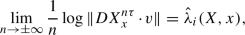
  for any and $i=1,\dots ,k(x)$. We also have a multiplicity one for the Lyapunov exponent $\hat{\lambda }_{i_0}(X,x)=0$.

Remark 2.9

A ‘Lyapunov exponent’ is constant along an orbit even when, for the transition from y to a point $x=X^\tau (y)$, the map $DX_y^\tau$ does not exist. In fact, we can use the broader definition of Lyapunov exponent (cf. [7]) and the fact that the mentioned transition is bounded by some constant depending on ${{\,\textrm{lip}\,}}(X)$ and $\tau$. Moreover, the Lyapunov exponents fulfill a property similar to what Abramov’s formula says about the metric entropy. We have $\lambda (X^t)=|t|\lambda (X^1)$ so it is irrelevant to choose other time-t flow to evaluate the Lyapunov exponents.

Let ${\lambda }_{1}(X,x)\geqslant \cdots \geqslant {\lambda }_{d}(X,x)$ denote the d Lyapunov exponents counted with multiplicity and set . The set $\{{\lambda }_{i}(X,x)\}_{i=1,\dots , d}$ is called the Lyapunov spectrum of X at x. When all Lyapunov exponents are equal we say that the Lyapunov spectrum is trivial. Since we have

$$\begin{aligned} \underset{n\rightarrow +\infty }{\lim }\,\frac{1}{n}\log |{\det DX^n_x}|=\sum _{i=1}^{d}\,\lambda _i(X,x), \end{aligned}$$

(2.7)

and in the divergence-free context $|{\det DX^n_x}|=1$, then being all equal means being all equal to 0. Due to the fact that for any of these subspaces $E^{i}_{x}\subset T_{x}M$, the angle between this space and ${\mathbb {R}}X(x)$ along the orbit has sub-exponential growth, that is

$$\begin{aligned} \lim _{n\rightarrow {\pm {\infty }}}\,\frac{1}{n}\log \sin \measuredangle \bigl (E^{i}_{X^{n\tau }(x)},{\mathbb {R}}X(X^{n\tau }(x))\bigr )=0, \end{aligned}$$

(2.8)

we conclude that the Lyapunov exponent $\hat{\lambda }_{i}(x)$ for $DX^{\tau }$ with associated subspace $E^i_x$ is also a Lyapunov exponent for $P_{X}^\tau$ associated to subspace $N^{i}_{x}=\Pi _x(E^i_x)$, $i \in \{1,\dots ,k(x)\}$, where $\Pi _x$ is the projection into $N_{x}$. In resume we have the following reformulation of Theorem 2.8.

Theorem 2.10

(Oseledets theorem for the linear Poincaré flow) Let $X\in \mathfrak {X}^{0,1}_{\nu ,\ell }(M)$ and $\tau >0$, then there is a $\nu$-full measure subset such that, for all :

• (1) there exists a $P^\tau _X$-invariant splitting of the fiber , with $1\leqslant k(x)\leqslant d-1$, along the orbit of x, and

• (2) there exist real numbers $\hat{\lambda }_{1}(f,x)>\dots >\hat{\lambda }_{k(x)}(f,x)$ called Lyapunov exponents, such that

  

  for any and $i=1,\dots ,k(x)$.

Remark 2.11

As the Lyapunov exponent in the vector field direction is 0, i.e. $\lambda _{i_0}=0$, and along this direction no metric entropy is added, then in (1.1) of Theorem A we have that $h_\nu (X)$ is equal to the entropy of the linear Poincaré time-1 map. Moreover, the right-hand side of (1.1) can be written as $\int _M \sum _{i=1}^{{d-1}}\lambda _i^+(P_X^1,x)\, d\nu (x)=\int _M \sum _{i=1}^d\lambda _i^+(DX^1,x)\, +\lambda _{i_0}(X,x)\,d\nu (x)$.

Now we present some multilinear algebra for the linear Poincaré map. The $k^\textrm{th}$ exterior power of the normal space N, denoted by , is a $\left( {\begin{array}{c}d-1\\ k\end{array}}\right)$-dimensional vector space. Let $\{e_{j}\}_{j\in J}$ ($\#\, J=d-1$) be an orthonormal basis of N, then the family of exterior powers for $j_{1}<\dots <j_{k}$ with $j_{\alpha }\in J$ forms an orthonormal basis of . Given $P_{X}^{t}(x):N_{x}\rightarrow N_{X^{t}(x)}$ we define

This formalism of multilinear algebra reveals to be the adequate to prove Theorem B. This is because we can recover the spectrum and the splitting information of the dynamics of from the one obtained by applying Oseledets’ theorem to $P_{X}^t(x)$. This is precisely the meaning of the next theorem [1, Theorem 5.3.1]. For a deeper discussion of exterior power algebra see [1, Section 3.2.3].

Theorem 2.12

(Oseledets theorem for the exterior power operator) The Lyapunov exponents $\lambda _{i}^{\wedge k}(x)$ for $i\in \{1,\dots ,(_{\,\,\,k}^{d-1})\}$ (repeated with multiplicity) of the $k^\textrm{th}$ exterior power operator are numbers of the form:

$$\begin{aligned} \sum _{j=1}^{k}\,\lambda _{i_{j}}(x),\quad \text{ where }\;\; 1\leqslant i_{1}< \cdots <i_{k}\leqslant d-1. \end{aligned}$$

This nondecreasing sequence starts with

• $\lambda _{1}^{\wedge k}(x)=\lambda _{1}(x)+\lambda _{2}(x)+\dots +\lambda _{k}(x)$, and ends with

• $\lambda _{q(k)}^{\wedge k}(x)=\lambda _{d-k}(x)+\lambda _{d+1-k}(x)+\dots +\lambda _{d-1}(x)$.

Take an Oseledets basis $\{e_{1}(x),\dots ,e_{d-1}(x)\}$ of $N_{x}$ such that $e_{i}(x)\in N_{x}^{\ell }$ for

$$\begin{aligned} \dim (N_{x}^{1})+\cdots +\dim (N_{x}^{\ell -1})<i\leqslant \dim (N_{x}^{1})+\cdots +\dim (N_{x}^{\ell }). \end{aligned}$$

Then the Oseledets space of is the subspace of which is generated by the k-vectors

Now we will consider the integrated upper Lyapunov exponent of the exterior power of the linear Poincaré map. Fixing $\tau >0$ we consider the following function:

(2.9)

In the same way we define the function , where $\Gamma \subseteq M$ is an $X^{t}$-invariant set, defined by

Let $\Sigma _{k}(X,x)$ denote the sum of the first k Lyapunov exponents of X, that is $\Sigma _{k}(X,x)=\lambda _{1}(X,x)+\dots +\lambda _{k}(X,x)$. It is an easy consequence of Theorem 2.12 (recall (2.7)) that for $k=1,\dots ,d-2$ we have and so , for any $X^t$-invariant set $\Gamma$. By using [11, Proposition 2.2] we get immediately that

concluding, from Lemma 2.7, that for all $k\in \{1,\dots ,d-2\}$, the function (2.9) is an upper semicontinuous function when the domain is endowed with the topology.

2.6 Dealing with singularities

In the next section we will see that small tailor made perturbations cause a decrease on the Lyapunov exponents. Yet, to perform these perturbations we need ‘time’ along the orbit and consequently the singularities, as equilibrium points, can make our task difficult. We will now see how we can rule out singularities in a sense that they typically represent a zero measure set. Given $X\in \mathfrak {X}_{\nu }^{1}(M)$, we observe that the hypothesis holds if all the singularities of X are hyperbolic, thus from classical results in [34], it is satisfied for a $C^1$-open⁴ and $C^1$-dense subset of ${\mathfrak {X}^{1}_{\nu }(M)}$. We say that $x\in M$ is a hyperbolic singularity for $X\in \mathfrak {X}_{\nu }^{1}(M)$ if the spectrum of $DX_x$ has neither pure complex nor zero as an eigenvalue. It is well known that a hyperbolic singularity is stable/persistent and moreover is isolated. Thus, hyperbolicity is a fundamental tool for checking whether a singularity is indeed an isolated singularity in the $C^r$ ($r\geqslant 1$) case. Basically, a similar statement holds for the Lipschitz class. However, as hyperbolicity is linked to differentiability, we must characterize a singularity being isolated through a broader analysis. Indeed, hyperbolicity is basically transversality and this property behaves in a similar way in the Lipschitz topology. We observe that thickening from the Lipschitz to the $C^0$-topology still captures the persistence of transversality but the ‘unicity’ is lost. Therefore, being isolated can no longer be guaranteed, as the reader can easily see. The next trivial example is illuminating.

Example 2.13

The Lipschitz function f defined by $f(x)=2x$ if $x\geqslant 0$ and $f(x)=3x$ if $x\leqslant 0$ is not derivable at the fixed point 0. Nevertheless, the fixed point is isolated under Lipschitz perturbations.

Let us consider the following observations:

• (1) The stability of elliptic singularities in divergence-free vector fields only happens when $\dim (M) = 2$. In fact pure complex eigenvalues (the elliptic case) persists under perturbations within the conservative setting. As we are considering $\dim (M)\geqslant 3$ we only have to deal with stable hyperbolic singularities (see [34] for more details).

• (2) Hyperbolic singularities are -stable in a sense that have a unique analytic continuation under perturbations. Notice that we are not saying that the continuation $\hat{x}$ of x for the perturbed $\widehat{X}\in \mathfrak {X}^{1}_{\nu }(M)$ is a hyperbolic singularity, because $D\widehat{X}_{\hat{x}}$ may not even exist. Still we get $\widehat{X}(\hat{x})=\textbf{0}$ and there exists a -open set containing $\hat{x}$ as the only singularity of $\hat{X}$.

• (3) Let be given $X\in \mathfrak {X}^{1}_{\nu }(M)$, $x\in M$ such that $X(x)=\textbf{0}$ and U an arbitrarily small open neighborhood of x. Then there exists an arbitrarily -close vector field $\widehat{X}\in \mathfrak {X}^{1}_{\nu }(M)$ such that $\widehat{X}(\hat{x})=\textbf{0}$, $\hat{x}$ is the only singularity in U, $D\widehat{X}_{\hat{x}}$ exists and $\hat{x}$ is hyperbolic for $\widehat{X}$. The conclusion is trivial when $DX_x$ exists and x is hyperbolic.

Let $X\in \mathfrak {X}_{\nu }^{0,1}(M)$. If all the singularities of X are hyperbolic, then they form a finite set, therefore with $\nu$-measure zero. Let $\widetilde{M}_X$ be the Rademacher points and be the set of singularities of X. We are only interested in the case when . In this case we cannot have hyperbolicity in the whole set . Yet, a small -perturbation can be made so that all singularities are of hyperbolic type and for this perturbed vector field $\widehat{X}\in \mathfrak {X}^{1}_{\nu }(M)$ we have .

3 Proof of Theorem B

3.1 Toolbox for realizable sequences

Our proof depends on the fact that the absence of a dominated splitting allows the Lyapunov exponents to decrease after a small perturbation. Once we have no dominated splitting then we can rotate the unstable Oseledets fiber until it reaches the stable Oseledets fiber mixing the rates of expansion and contraction. This idea goes back at least as far as the 1970s and the Soviet school (see e.g. [27]). In our precise context we refer to Mañé’s seminal ideas [22, 24] culminated in the outstanding work by Bochi and Viana [11] for the discrete case. For the continuous-time case, see [4, 6].

The main tool to realize, implement and make explicit such perturbations is a flowbox theorem for the divergence-free Lipschitz vector fields which has been proved recently. Let us recall this result but first we begin by defining some useful objects. We say that two vector fields $X_1:U_1\rightarrow TU_1$ and $X_2:U_2\rightarrow TU_2$ are locally topologically conjugate near $p_1\in U_1$ and $p_2\in U_2$ if there exist two open neighborhoods $O_i\ni p_i$ ($i=1,2$) and a homeomorphism $\phi :O_1\rightarrow O_2$ with $\phi (p_1)=p_2$ such that for any $x\in O_1$ and a small interval I containing 0 the integral curve $\sigma _x:I\rightarrow O_1$ defined by $\sigma _x(0)=x$ and $\frac{d}{dt}\sigma _x(t)=X_1(\sigma _x(t))$ for all $t\in I$ (i.e. defined by $X_1^{t}(x)$ for $t\in I$) is a solution associated to $X_1$ if and only if the integral curve is a solution associated to $X_2$.

Theorem 3.1

(Flowbox theorem for Lipschitz divergence-free vector fields [5]) Let be given $X\in \mathfrak {X}_{\nu }^{0,1}(M)$, a non-singular point $p_1\in {M}$ and the trivial vector field $T(\hat{x}_1,\hat{x}_2,\dots ,\hat{x}_{{d}})=(1,0,\dots ,0)$ on canonical coordinates $(\hat{x}_1,\hat{x}_2,\dots ,\hat{x}_{{d}})$ of $\,{\mathbb {R}}^d$. Then:

• (i) X and T are locally topologically conjugate near $p_1$ and $p_2=\hat{0}$. The homeomorphism $\phi$ which gives the conjugacy is a lipeomorphism.

• (ii) X and $T_c=c T$ are locally topologically (volume-preserving) conjugate near $p_1$ and $p_2=\hat{0}$ for some $c=c(X,p_1)>0$. The homeomorphism $\Phi$ which gives the conjugacy is a volume-preserving lipeomorphism.

For the reader’s convenience, we repeat the relevant material from [6] omitting most of the proofs, thus making the text self-contained. As in [6, Definition 4.1] the realizable sequences will be a key object to obtain Theorem B. By modified volume-preserving we mean the volume on the $(d-1)$-dimensional transversal section whose measure is denoted by $\overline{\nu }$. This is a simple point regarding that $\overline{\nu }$ is not invariant but by considering a density given by the direction of the flow we obtain invariance (see [6, Section 2.4]). The set represents a flowbox obtained by the $X^t$-saturation of the set U contained in a transverse section through x.

Definition 3.2

Given $X\in \mathfrak {X}_{\nu }^{0,1}(M)$, $\varepsilon >0$, $\kappa \in (0,1)$, $\ell \in {\mathbb {N}}$, and a non-periodic point x, we say that the modified volume-preserving sequence of linear maps $L_{j}:N_{X^{j}(x)}\rightarrow {N_{X^{j+1}(x)}}$ for $j=0,\dots ,\ell -1$ is an $(\varepsilon ,\kappa )$-realizable sequence of length $\ell$ at x if the following occurs: For all $\gamma >0$, there is $r>0$ such that for any $(d-1)$-manifold (tangent to $N_x$) and any non-empty open set , there exist a measurable set $K\subseteq {U}$ and $Y\in \mathfrak {X}_{\nu }^{0,1}(M)$ satisfying the conditions:

• (a) ;

• (b) $\Vert Y-X\Vert _{0,1}<\varepsilon$;

• (c) $Y=X$ outside ; and

• (d) if $y\in {K}$, then $\Vert P^{1}_{Y}(Y^{j}(y))-L_{j}\Vert <\gamma$ for all $j=0,1,\dots ,\ell -1.$

Let ${\mathbb {R}}^d$ be the Euclidean space in canonical coordinates $(\hat{x}_1,\hat{x}_2,\dots ,\hat{x}_{{d}})$. We denote the $(d\,{-}\,1)$-dimensional ball with radius r in the subspace described by $\hat{x}_1=0$ by $B^{{d}-1}(\textbf{0},r)$. That is $B^{{d}-1}(\textbf{0},r)$ is the set of points $(0,\hat{x}_2,\dots ,\hat{x}_{{d}})$ such that $\Vert (0,\hat{x}_1,\hat{x}_2,\dots ,\hat{x}_{{d}})\Vert \leqslant r$. The following result is the basic tool in order to build realizable sequences.

Lemma 3.3

Given the trivial vector field T written in canonical coordinates of ${\mathbb {R}}^d$, $\varepsilon >0$, $r>0$ and $\kappa \in (0,1)$, there exists $\xi _{0}>0$ such that for any $\xi \in (0,\xi _{0})$, for $\textbf{0}\in {\mathbb {R}}^d$ and any 2-dimensional vector space $V_{\textbf{0}} \subset \langle (0,\hat{x}_2,\dots ,\hat{x}_{{d}})\rangle$ there exists a smooth vector field Y such that:

• (a) $Y=T$ outside the flowbox cylinder ;

• (b) ;

• (c) $\Vert Y-T\Vert _{0,1}<\varepsilon$; and

• (d) where and $\mathfrak {R}_\xi$ is the rotation of angle $\xi$ in $V_{\textbf{0}}$ and the identity in the complementary subspace (i.e. a ‘cylindrical rotation’).

Proof

For simplicity of presentation, we assume that $V_{\textbf{0}} = \langle (0,\hat{x}_2,\hat{x}_3,0,\dots ,0)\rangle$ and also abusively assume that $c=1$ in (ii) of Theorem 3.1. Consider the bump-functions g and G defined by:

• $g:{\mathbb {R}}\rightarrow {{\mathbb {R}}}$ is a $C^{\infty }$-function such that $g(t)=0$ for $t<0$, $g(t)=t$ for $t\in [\eta ,1-\eta ]$ for $\eta >0$ small, $g(t)=1$ for $t\geqslant {1-\eta /2}$, $\dot{g}\leqslant 1$ and $\ddot{g}\leqslant 2\eta ^{-1}$, and

• $G:{\mathbb {R}}\rightarrow {[0,1]}$ is a $C^{\infty }$-function such that $G(\rho )=1$ for $\rho \leqslant {r\sqrt{1-{\kappa }/{2}}}$, $G(\rho )=0$ for $\rho \geqslant {r}$ and .

Let $\rho =\sqrt{{\hat{x}_2}^{2}+{\hat{x}_3}^{2}}$ and consider the rotation flow $R_{\xi {g(t)}G(\rho )}(0,{\hat{x}_2},{\hat{x}_2},0,\dots ,0)$ acting on $V_{\textbf{0}}$, which we denote by and defined by

Notice that . Denote . Through a simple calculation we obtain that

(3.1)

We note that and outside $\mathscr {F}^{1}_{T}(\textbf{0})(B^{{d}-1}(\textbf{0},r))$. We define

Hence . We are left to see that $\Vert Y-T\Vert _{0,1}<\varepsilon$ and for that we notice that . We will show that the perturbation defined in (3.1) is such that

where stands for the $C^1$-Whitney topology. Clearly, the $C^0$-norm is controlled essentially by the size of $\xi$ so let us estimate the $C^1$-norm. Using the product rule on the derivative of the perturbation we get

(3.2)

Observe that the gradient is equal to

Let us see that all the terms in (3.2) are controlled. In the second item below we use the polar coordinates representation $\hat{x}_2=\widetilde{r}\cos \beta$ and $\hat{x}_3=\widetilde{r}\sin \beta$.

We have which is controlled by the size of $\xi$. We also have

which is also controlled by the size of $\xi$. Hence, all the items (a)–(d) are fulfilled and the lemma is proved. $\square$

The next result follows directly from combining Theorem 3.1 and Lemma 3.3. Firstly, Theorem 3.1 provides us with good trivial coordinates and secondly Lemma 3.3 allows us to perform the perturbations which essentially will be done into several small balls that fill the open set U proclaimed in Definition 3.2 (see [6, Lemma 5.3]).

Lemma 3.4

Given $X\in \mathfrak {X}_{\nu }^{0,1}(M)$, $\varepsilon >0$ and $\kappa \in (0,1)$, there exists $\xi _{0}>0$ such that for any $\xi \in (0,\xi _{0})$, any $x\in M$ (non-periodic or with period $>1$) and any 2-dimensional vector space $V_x \subset N_{x}$ one has that the time-1 map is an $(\varepsilon ,\kappa )$-realizable sequence of length 1 at x, where and $\mathfrak {R}_\xi$ is the rotation of angle $\xi$ in $V_x$.

The next result is the key step that allows us to mix the Oseledets directions in the absence of a dominated splitting. This is the rotation (using Lemma 3.4) from the unstable Oseledets fiber to the stable Oseledets fiber referred to in the first paragraph of this section.

Proposition 3.5

Given $X\in \mathfrak {X}_{\nu }^{0,1}(M)$, $\varepsilon >0$ and $\kappa \in (0,1)$, there exists $m_{0}\in {\mathbb {N}}$ such that for every $m\geqslant m_{0}$ the following property holds. For any non-periodic point $x\in \widetilde{M}_{X}$ with a splitting , $t \in {\mathbb {R}}$ and $j \in \{1,\dots ,d-2\}$ fixed, satisfying

(3.3)

there exist $(\varepsilon _i,\kappa _i)$-realizable sequences of length $\ell _i \geqslant 1$ at $X^{\tau _i}(x)$, with $0 \leqslant i \leqslant b \leqslant m$, $\sum _{i=0}^{b}\ell _i=m$ and $\tau _i=\sum _{j=1}^{i-1}\ell _j$, denoted by $\{L_{i}\}_{i=1}^{b}$ and vectors and such that:

• (a) the concatenation of the b-realizable sequences is an $(\varepsilon ,\kappa )$-realizable sequence of length m at x, and

• (b) .

3.2 Concluding the proof of Theorem B

Once we have established Proposition 3.5 it remains:

$\lozenge$:

First, use Proposition 3.5 to decrease the Lyapunov exponent in a single orbit by showing that for every $\varepsilon ,\delta >0$, $k\in \{1,\dots ,d-2\}$ and $\nu$-almost every point x in a set without dominated splitting with $\dim E=k$ we can find a ‘time’ $t>\widetilde{T}(x)$ such that there exists a modified volume-preserving sequence of linear maps $L_{j}:N_{X^{j}(x)}\rightarrow {N_{X^{j+1}(x)}}$ for $j=0,\dots ,t-1$ which is an $(\varepsilon ,\kappa )$-realizable sequence of length t at x satisfying

This local procedure uses the lack of domination (3.3) and also the different Lyapunov exponents to cause a decrease of the largest Lyapunov exponent of the $k^\textrm{th}$ exterior power of the linear Poincaré map by a small -perturbation.

$\blacklozenge$:

Second, we generalize the previous construction from a point to a large measure set using a Kakutani’s tower argument. It is possible to prove that, given any $\varepsilon ,\delta >0$, and $k \in \{1,\dots ,d-2\}$, there exists $Y\in \mathfrak {X}_{\nu }^{0,1}(M)$, which is $\varepsilon$--close to X, such that

$$\begin{aligned} \int _M\Sigma _k(Y,x)\,d\nu (x)<\int _M\Sigma _k(X,x)\,d\nu (x)- 2J_k(X)+\delta , \end{aligned}$$

where $J_k(X)$ is the jump of the function, namely, the integral of $\lambda _k(X,x)-\lambda _{k+1}(X,x)$ over a set without domination between the Oseledets directions associated to $\lambda _k(X,x)$ and $\lambda _{k+1}(X,x)$. Of course, if this set without dominated splitting has zero $\nu$-measure we apply this argument again, with k replaced by $k+1$ until we reach $d-2$.

Finally, to prove Theorem B we follow ipsis litteris the arguments in [11, p. 1467]. More precisely, for $k \in \{1,\dots ,d-2\}$ let be the subset corresponding to the points of continuity of the map defined in (2.9). Take . It is well known that the sets are residual subsets and so is . If then, by the definition of this set and by $\blacklozenge$ above, we obtain that $J_k(X)=0$. Therefore $\lambda _k(X,x)=\lambda _{k+1}(X,x)$ for a.e. x in a set without a dominated splitting. For the subset is defined by the Oseledets regular points without any dominated splitting between any fiber, and the set is defined by the Oseledets regular points with some kind of dominated splitting. Hence, if then all the Lyapunov exponents of x are equal to zero and this ends the proof of Theorem B.

4 Proof of Theorem C

4.1 Preliminary results

We have divided the proof of Theorem C into three lemmas focusing on a suitable choice of the decomposition given by the Oseledets theorem. The idea of the proof of the first lemma goes back at least as far as [20, Lemma 3] where this was proved under a uniform hyperbolic context. It was subsequently proved in [36, Lemma 3.3] under the weaker assumption of a dominated splitting and in [8, Lemma 6.1] it was again proved but in the even weaker context of lipeomorphisms. We will state it and observe that its proof follows closely the arguments in [8, 23, 36]. In order to present this lemma let us first recall some definitions. The formulation of item (ii) of Lemma 4.1 is equivalent to the one in [8, Lemma 6.1] but substantially different from the original one in [23, 36] that was based on $C^1$-regularity which is not taken for granted for Lipschitz vector fields. The motivation of using the $\ell$-property defined in Sect. 2.4 lies in the fact that the next result remains operational. Recalling again Abramov’s formula and Remark 2.9 we perform our study for the time-1 Poincaré map and so our proof is very close to the proof of the discrete-time case. Indeed, we are considering metric entropy and Lyapunov exponents, on which the usual considerations about having an ${\mathbb {R}}$-action instead of a ${\mathbb {Z}}$-action does not need a specific analysis. Loosely speaking the directions of the vector field do not contribute to the change of both entropy and Lyapunov exponents.

Given a normed space and a splitting , we define $\gamma (E,F)$ as the maximum of the norms of the projections ($i=1,2$). A subset is said to be an (E, F)-graph if there exists an open set $U\subset F$ and a Lipschitz map $\psi :U\rightarrow E$ such that $G=\{x+\psi (x)\,{:}\, x\in U\}$. The dispersion of the graph G is given by ${{\,\textrm{lip}\,}}_U(\psi )=\sup _{x\not =y\in U}\frac{\Vert \psi (x)-\psi (y)\Vert }{\Vert x-y\Vert }$.

Lemma 4.1

([8, Lemma 6.1]) Let $\alpha , \beta , c,\delta >0$ be such that

Let , be two finite-dimensional normed spaces, a splitting such that $\gamma (E,F)\leqslant \alpha$ and a Lipschitz map where is defined and satisfying the following properties:

• (i) is an isomorphism and ;

• (ii) denoting and and for some small $r>0$ and $(x,y)\in B(0,r)$, we have

  

  with remainders p(x, y) and q(x, y) having Lipschitz constants less than $\delta$;

• (iii) , and

• (iv) ,

then is a -graph with dispersion $\leqslant c$, for every (E, F)-graph $G\subset B(0,r)$ with dispersion $\leqslant c$.

When applying previous lemma and according to item (iii) above we need to have a set with a dominated splitting. This set will be precisely the set of Theorem B. As the dominated splitting is w.r.t. the linear Poincaré map we will take and of Lemma 4.1 to be, respectivelly, the Poincaré map and the linear Poincaré map $P_X^t(x)$ associated to a certain $X\in \mathfrak {X}_{\nu }^{0,1}(M)$. We notice that we are not able to proceed with the arguments considering the tangent map $DX^t$ because there is no reason to have a dominated splitting of TM for $DX^t$. Recall that by (2.8) the only control we have over the angle is that the convergence to zero (if exists) is not very fast. The existence of a convergence to zero of this angle forbids a dominated splitting.

Let $f:M\rightarrow M$ be a homeomorphism, $r>0$, $x\in M$ and $n\in {\mathbb {N}}$. Let

$$\begin{aligned} B_n(f,r,x)=\bigcap _{j=0}^n f^{-j}(B(f^{j}(x),r)) \end{aligned}$$

be the Bowen ball. Define also

(4.1)

In [20, 21], it was proved that

$$\begin{aligned} h_\nu (f)\geqslant \sup _{r>0}\int _M h_\nu (f,r,x)\, d\nu (x). \end{aligned}$$

(4.2)

From Lemmas 4.1, 2.2 and a simple induction argument we deduce the following result. For details see [36, Lemma 3.4].

Lemma 4.2

Let $X\in \mathfrak {X}_{\nu }^{0,1}(M)$ and be an $X^t$-invariant set. If there is a 1-dominated splitting on for the linear Poincaré map, say , then for any $c>0$, there exists $r>0$ such that for every and any $(E_x,F_x)$-graph with dispersion $\leqslant c$ contained in a Bowen ball $B_n(X^1,x,r)$, $n\geqslant 1$, is a -graph with dispersion $\leqslant c$.

Take a vector field $X\in \mathfrak {X}_{\nu }^{0,1}(M)$, $\varepsilon >0$ and a $\nu$-full measure set $\Sigma \subseteq \widetilde{M}_{X^1}$ with an $m_x$-dominated splitting for $P_X^1$ of a certain fixed index. Consider $N_\varepsilon \in {\mathbb {N}}$ sufficiently large in order to have $\nu (\Sigma _\varepsilon )>1-\varepsilon$, where $\Sigma _\varepsilon =\{x\in \Sigma \,{:}\, m_x\leqslant N_\varepsilon \}$. Observe that , for $N=N_\varepsilon !$, is such that displays a 1-dominated splitting for say for $P_X^N$ (see [36, p. 1430]). Recall that a dominated splitting can be extended to the closure of $\Sigma _\varepsilon$ wherever it is defined⁵ and moreover it varies continuously with the point.

Lemma 4.3

Given f, N and $\varepsilon$ as above, there exists $r>0$ such that for $\nu$-a.e. $x\in \Sigma _\varepsilon$ we have

(4.3)

Proof

Fix $a,c>0$ such that if $x\in \Sigma _\varepsilon$ and $y\in B(x,a)$ is a $\nu$-generic Rademacher point, then for any linear subspace $G\subseteq N_x$ which is an $(E_x,F_x)$-graph with dispersion $\leqslant c$, we have from Remark 2.2 that

$$\begin{aligned} \bigl | {\log |{\det Df_y}|_{G}}\bigr |- \log |{\det Df_x|_{F}}|<\varepsilon . \end{aligned}$$

and so

(4.4)

Providing Lemma 4.2 with $(\text {mod} \,\nu )$, the 1-dominated splitting and the $c>0$ above, there exists $r>0$ such that for every and any $(E_x,F_x)$-graph G with dispersion $\leqslant c$ contained in a Bowen ball $B_n(f,x,r)$, $n\geqslant 1$, $f^n(G)$ is a -graph with dispersion $\leqslant c$.

Given $x\in \Sigma _\varepsilon$ and $y\in E_x$, we denote by $\nu _E$ the volume measure in $E_x$ and by $\nu _F$ the volume measure in $y+F_x$. There exists $B>0$ such that the disintegration holds for all $n\geqslant 1$:

(4.5)

where . Here notice that B incorporates also the length of the 1-dimensional component transversal to the $(d\,{-}\,1)$-dimensional subspace associated to . From (4.1) and (4.5) we get

Hence, Lemma 4.3 is proved once we obtain that for $\nu$-a.e. $x\in \Sigma _\varepsilon$ the following inequality holds:

(4.6)

Considering that and using Lemma 4.2 we obtain that is a -graph with dispersion $\leqslant c$. Given $r\in (0,a)$, we take

Notice that for $f^n(x)\in \Sigma _\varepsilon$ we have . Thus,

(4.7)

For any $j=0,1,\dots ,n$ we have , and so given any , we have $d(f^j(z),f^j(x))<a$ for all $j=0,1,\dots ,n$. By (4.7) we obtain

which is equivalent to

Taking limits and recalling that $f=X^N$ we obtain

and (4.6) is proved and so is the lemma. $\square$

4.2 Proof of Theorem C

We would like to show that for a given $X\in \mathfrak {X}_{\nu }^{0,1}(M)$ if for $\nu$-a.e. $x\in M$ there is an $m_x$-dominated splitting for the linear Poincaré map along the orbit of x (where $m:M\rightarrow {\mathbb {N}}$ is an $X^t$-invariant measurable function), then

Notice that it suffices to prove the theorem for a certain fixed dimension of F. Remark 2.11 sheds some light on the fact that we focus on a dominated splitting for the linear Poincaré map.

Let $f,N,\varepsilon$ and $r>0$ be given like in Lemma 4.3. Let $C={{\,\textrm{lip}\,}}(X)$, and from Gronwall’s inequality we get $\Vert DX_x^t\Vert \leqslant e^{t\Vert DX_x\Vert }\leqslant e^{t{{\,\textrm{lip}\,}}(X)}=e^{tC}$ for $\nu$-a.e. x. We have

Hence, recalling the Abramov formula,

and since $\varepsilon$ is arbitrarily small, Theorem C is proved.

References

Abramov, L.M.: On the entropy of a flow. Dokl. Akad. Nauk SSSR 128, 873–875 (1959) (in Russian)
Artigue, A.: Lipschitz perturbations of expansive systems. Discrete Contin. Dyn. Syst. 35(5), 1829–1841 (2015)
Barreira, L., Pesin, Ya.: Nonuniform Hyperbolicity. Encyclopedia of Mathematics and Its Applications, vol. 115. Cambridge University Press, Cambridge (2007)
Bessa, M.: The Lyapunov exponents of zero divergence three-dimensional vector fields. Ergodic Theory Dynam. Systems 27(5), 1445–1472 (2007)
Bessa, M.: The flowbox theorem for divergence-free Lipschitz vector fields. C. R. Math. Acad. Sci. Paris 355(8), 881–886 (2017)
Bessa, M., Rocha, J.: Contributions to the geometric and ergodic theory of conservative flows. Ergodic Theory Dynam. Systems 33(6), 1709–1731 (2013)
Bessa, M., Silva, C.M.: Dense area-preserving homeomorphisms have zero Lyapunov exponents. Discrete Contin. Dyn. Syst. 32(4), 1231–1244 (2012)
Bessa, M., Silva, C., Vilarinho, H.: Stretching a generic Pesin’s entropy formula. J. Stat. Phys. 173(5), 1523–1546 (2018)
Bessa, M., Torres, M.J., Varandas, P.: On the periodic orbits, shadowing and strong transitivity of continuous flows. Nonlinear Anal. 175, 191–209 (2018)
Bessa, M., Varandas, P.: On the entropy of conservative flows. Qual. Theory Dyn. Syst. 10(1), 11–22 (2011)
Bochi, J., Viana, M.: The Lyapunov exponents of generic volume-preserving and symplectic maps. Ann. Math. 161(3), 1423–1485 (2005)
Buhovsky, L., Seyfaddini, S.: Uniqueness of generating Hamiltonians for topological Hamiltonian flows. J. Symplectic Geom. 11(1), 37–52 (2013)
Cornfeld, I.P., Fomin, S.V., Sinai, Ya.G.: Ergodic Theory. Grundlehren der Mathematischen Wissenschaften, vol. 245. Springer, New York (1982)
Dou, D., Fan, M., Qiu, H.: Topological entropy on subsets for fixed-point free flows. Discrete Contin. Dyn. Syst. 37(12), 6319–6331 (2017)
Federer, H.: Geometric Measure Theory. Die Grundlehren der mathematischen Wissenschaften, vol. 153. Springer, New York (1969)
Hartman, P.: Ordinary Differential Equations. Classics in Applied Mathematics, vol. 38, 2nd edn. SIAM, Philadelphia (2002)
Irwin, M.C.: Smooth Dynamical Systems. Advanced Series in Nonlinear Dynamics, vol. 17. World Scientific, River Edge (2001)
Katok, A.: Fifty years of entropy in dynamics: 1958–2007. J. Mod. Dyn. 1(4), 545–596 (2007)
Maleva, O., Preiss, D.: Directional upper derivatives and the chain rule formula for locally Lipschitz functions on Banach spaces. Trans. Amer. Math. Soc. 368(7), 4685–4730 (2016)
Mañé, R.: A proof of Pesin’s formula. Ergodic Theory Dynam. Systems 1(1), 95–102 (1981)
Mañé, R.: Errata to: “A proof of Pesin’s formula’’. Ergodic Theory Dynam. Systems 3(1), 159–160 (1981)
Mañé, R.: Oseledec’s theorem from the generic viewpoint. In: Ciesielski, Z., Olech, C. (eds.) Proceedings of the International Congress of Mathematicians, vol. 1, 2 (Warsaw, 1983), pp. 1269–1276. PWN, Warsaw (1984)
Mañé, R.: Ergodic Theory and Differentiable Dynamics. Ergebnisse der Mathematik und ihrer Grenzgebiete, vol. 8. Springer, Berlin (1987)
Mañé, R.: The Lyapunov exponents of generic area preserving diffeomorphisms. In: Ledrappier, F., et al. (eds.) International Conference on Dynamical Systems (Montevideo, 1995). Pitman Res. Notes Math. Ser., vol. 362, pp. 110–119. Longman, Harlow (1996)
Morales, C.A., Thieullen, P., Villavicencio, H.: Lyapunov exponents on metric spaces. Bull. Aust. Math. Soc. 97(1), 153–162 (2018)
Moser, J.: On the volume elements on a manifold. Trans. Amer. Math. Soc. 120, 286–294 (1965)
Novikov, V.L.: Almost reducible systems with almost periodic coefficients. Mat. Zametki 16, 789–799 (1974) (in Russian)
Oh, Y.-G.: The group of Hamiltonian homeomorphisms and continuous Hamiltonian flows. In: Fathi, A., et al. (eds.) Symplectic Topology and Measure Preserving Dynamical Systems. Contemporary Mathematics, vol. 512, pp. 149–177. American Mathematical Society, Providence (2010)
Oh, Y.-G., Müller, S.: The group of Hamiltonian homeomorphisms and \(C^0\)-symplectic topology. J. Symplectic Geom. 5(2), 167–219 (2007)
Oseledets, V.I.: A multiplicative ergodic theorem. Characteristic Ljapunov, exponents of dynamical systems. Trans. Moscow Math. Soc. 19, 197–231 (1968)
Pacifico, M.J., Vieitez, J.L.: Lyapunov exponents for expansive homeomorphisms. Proc. Edinb. Math. Soc. 63(2), 413–425 (2020)
Palis, J., de Melo, W.: Geometric Theory of Dynamical Systems. Springer, New York (1982)
Pesin, Ya.B.: Characteristic Ljapunov exponents, and smooth ergodic theory. Uspehi Mat. Nauk 32(4)(196), 55–112 (1977) (in Russian)
Robinson, R.C.: Generic properties of conservative systems. Amer. J. Math. 92, 562–603 (1970)
Ruelle, D.: An inequality for the entropy of differentiable maps. Bol. Soc. Brasil. Mat. 9(1), 83–87 (1978)
Sun, W., Tian, X.: Dominated splitting and Pesin’s entropy formula. Discrete Contin. Dyn. Syst. 32(4), 1421–1434 (2012)
Sun, W., Vargas, E.: Entropy of flows, revisited. Bol. Soc. Brasil. Mat. (N.S.) 30(3), 315–333 (1999)
Tahzibi, A.: \(C^1\)-generic Pesin’s entropy formula. C. R. Math. Acad. Sci. Paris 335(12), 1057–1062 (2002)
Viterbo, C.: On the uniqueness of generating Hamiltonian for continuous limits of Hamiltonians flows. Int. Math. Res. Not. 2006, Art. No. 34028 (2006)
Viterbo, C.: Erratum to: “On the uniqueness of generating Hamiltonian for continuous limits of Hamiltonians flows”. Int. Math. Res. Not. 2006, Art. No. 38784 (2006)
Acknowledgements
The author thanks the referee for careful reading of the paper and for making constructive comments which helped improving the presentation.
Funding
Open access funding provided by FCT|FCCN (b-on).
Author information
Authors and Affiliations
Corresponding author
Additional information
Publisher's Note
Springer Nature remains neutral with regard to jurisdictional claims in published maps and institutional affiliations.
The author was partially supported by FCT—‘Fundação para a Ciência e a Tecnologia’, through Centro de Matemática e Aplicações (CMA-UBI), Universidade da Beira Interior, project UID/00212/2020, and partially supported by the Project ‘New Trends in Lyapunov Exponents’ (PTDC/MAT-PUR/29126/2017). The author thanks CMUP for providing necessary conditions in which this work was developed.
Rights and permissions
Open Access This article is licensed under a Creative Commons Attribution 4.0 International License, which permits use, sharing, adaptation, distribution and reproduction in any medium or format, as long as you give appropriate credit to the original author(s) and the source, provide a link to the Creative Commons licence, and indicate if changes were made. The images or other third party material in this article are included in the article’s Creative Commons licence, unless indicated otherwise in a credit line to the material. If material is not included in the article’s Creative Commons licence and your intended use is not permitted by statutory regulation or exceeds the permitted use, you will need to obtain permission directly from the copyright holder. To view a copy of this licence, visit http://creativecommons.org/licenses/by/4.0/.
About this article
Cite this article
Bessa, M. Lyapunov exponents and entropy for divergence-free Lipschitz vector fields. European Journal of Mathematics 9, 20 (2023). https://doi.org/10.1007/s40879-023-00611-6
Received:
Revised:
Accepted:
Published:
DOI: https://doi.org/10.1007/s40879-023-00611-6