On standing waves and gradient-flow for the Landau–De Gennes model of nematic liquid crystals

Abstract

The article treats the existence of standing waves and solutions to gradient-flow equation for the Landau–De Gennes models of liquid crystals, a state of matter intermediate between the solid state and the liquid one. The variables of the general problem are the velocity field of the particles and the Q-tensor, a symmetric traceless matrix which measures the anisotropy of the material. In particular, we consider the system without the velocity field and with an energy functional unbounded from below. At the beginning we focus on the stationary problem. We outline two variational approaches to get a critical point for the relative energy functional: by the Mountain Pass Theorem and by proving the existence of a least energy solution. Next we describe a relationship between these solutions. Finally we consider the evolution problem and provide some Strichartz-type estimates for the linear problem. By several applications of these results to our problem, we prove via contraction arguments the existence of local solutions and, moreover, global existence for initial data with small $L^2$-norm.

1 Introduction

There are different models describing nematic liquid crystals (we avoid long list of references, but refer to the recent one [25] that gives a very detailed panorama of the state of the art). We are interested in the Q-tensor model, i.e. De Gennes type model (see [1, 9, 16]) for a molecule in a flux of nematic liquid crystals, which is a state of matter intermediate between the solid state and the liquid one. Concerning the physical modeling of nematic liquid crystals, we refer to [1,2,3,4, 23, 25]. The model has been actively studied during the last years both on torus [7, 24], bounded domains [13], in ${\mathbb {R}}^n$ [17, 18], and in exterior domains [8, 19, 20]. In general the model is described by a system of Navier–Stokes equations and an equation for the Q-tensor:

where $Q=(q_{i j})_{i, j=1,2,3}$ and

We are looking for the functions

where $S_{0}(3, {\mathbb {R}})$ denotes the space of symmetric matrices with zero trace. The function u represents the velocity field of the molecules, p represents the pressure of the fluid and Q is the De Gennes Q-tensor.

In the model, F denotes the energy of liquid crystals and it is given by

where $a,b,c\in {\mathbb {R}}$ and is the Frobenius norm. It is easy to prove that

$$\begin{aligned} \partial F(Q)=aQ+b(Q^2)^{\mathrm{T}}+c|Q|^2Q \quad \text {for all}\;\; Q\in M(3,{\mathbb {R}}). \end{aligned}$$

In the case $u=0$ the model reduces to the gradient flow equation

$$\begin{aligned} \partial _{t} Q = \Delta _{x} Q-L[\partial F(Q)]. \end{aligned}$$

Our first goal is to find standing waves, i.e. solutions to the equation

(1)

for $Q\in H^1({\mathbb {R}}^3;S_0(3,{\mathbb {R}}))$.

We shall use the following parametrization for the matrices of $S_0(3,{\mathbb {R}})$:

$$\begin{aligned} Q(q(x))=\left( \begin{array}{llc} q_{1}(x) &{}\, q_{3}(x) &{}\, q_{4}(x) \\ q_{3}(x) &{}\, q_{2}(x) &{}\, q_{5}(x) \\ q_{4}(x) &{}\, q_{5}(x) &{}\,{} -q_{1}(x)-q_{2}(x) \end{array}\right) ,\quad q = (q_1,q_2, q_3,q_4,q_5). \end{aligned}$$

It can be proved that every critical point q of the following functional:

gives a matrix Q(q) which satisfies (1).

The part of our work, related to the stationary problem, was announced in [12]. However, for completeness we present the proofs or key points in the proofs, so that the article is self-contained.

2 Least energy solution

2.1 Existence of a least energy solution

We study the case $a>0$ and $c<0$.

Definition 2.1

Let $d\geqslant 3$, $n\geqslant 2$, $p=\frac{2d}{d-2}$, and

let q be a solution of the system

(2)

where $\alpha \in [0,1]$ and $e_1,e_2$ are the following vectors of ${\mathbb {R}}^n$:

and

We say that q is a least energy solution of (2) if and

where

Following [6], we consider a function which satisfies the following properties for $p=\frac{2d}{d-2}$:

• $G(0)=0$;

• $\limsup _{|v|\rightarrow +\infty } |v|^{-p}G(v)\leqslant 0$;

• $\limsup _{|v|\rightarrow 0} |v|^{-p}G(v)\leqslant 0$;

• there exists $\xi _0\in {\mathbb {R}}^n$ such that $G(\xi _0)>0$;

• for all $\gamma >0$ there exists $C_\gamma$ such that

  $$\begin{aligned} |G(v+w)-G(v)|\leqslant \gamma [|G(v)|+|v|^p]+C_\gamma [|G(w)|+|w|^p+1] \end{aligned}$$

  (3)

  for all $v,w\in {\mathbb {R}}^n$;

• there exists a constant $C>0$ such that

  $$\begin{aligned} g(v)\leqslant C+C|v|^{p-1} \quad \text {for all}\;\; v\in {\mathbb {R}}^n. \end{aligned}$$

In [6] the existence of a least energy solution is established for $\alpha =0$. We need a small generalization to show it for $\alpha \in [0,1]$.

Theorem 2.2

Let $\alpha \in [0,1]$, $d\geqslant 3$, $n\geqslant 2$ and $G:{\mathbb {R}}^n\rightarrow {\mathbb {R}}$ satisfy the above hypotheses, then there exists a least energy solution $q:{\mathbb {R}}^d\rightarrow {\mathbb {R}}^n$ of (2).

Proof

The proof is almost the same as in [6], so we just list the steps:

Step 1: Let us consider the problem

Let $\{q^j\}_j$ be a minimizing sequence for T, then $\{\nabla q^j\}_j$ is bounded in $L^2({\mathbb {R}}^d;{\mathbb {R}}^n)$ and $\{q^j\}_j$ is bounded in $L^p({\mathbb {R}}^d;{\mathbb {R}}^n)$. It can be proved also that, passing to a subsequence,

for .

Step 2: $\int G(q)\,dx=1$ and

In particular, $\nabla q^j\rightarrow \nabla q$ in $L^2({\mathbb {R}}^d;{\mathbb {R}}^n)$ and therefore $q^j\rightarrow q$ in $L^p({\mathbb {R}}^d;{\mathbb {R}}^n)$.

Step 3: Let ${\overline{q}}(x)=q(\theta x)$ with $\theta =\frac{d}{T(d-2)}$, then in there holds

$$\begin{aligned} {} -\Delta {\overline{q}}-\alpha (\Delta {\overline{q}}_1e_2+\Delta {\overline{q}}_2e_1)=g({\overline{q}})=\nabla G({\overline{q}}). \end{aligned}$$

Step 4: If is a solution of (2), then there holds

Step 5: For all non-zero and satisfying (2), we have

$$\begin{aligned} 0<\int |\nabla {\overline{q}}|^2+\alpha \nabla {\overline{q}}_1\nabla {\overline{q}}_2-G({\overline{q}})\,dx\leqslant \int |\nabla v|^2+\alpha \nabla v_1\nabla v_2-G(v)\,dx. \end{aligned}$$

Step 6: We have the following regularity result:

Theorem 2.3

Let be a solution of (2) with $g(q)\in L^1_{\mathrm{loc}}({\mathbb {R}}^d;{\mathbb {R}}^n)$, then it satisfies the following properties:

• $q\in W^{2,t}_{\mathrm{loc}}({\mathbb {R}}^d;{\mathbb {R}}^n)$ for any $t<\infty$;

• $q\in L^\infty ({\mathbb {R}}^d;{\mathbb {R}}^n)$;

• q tends to 0 as $|x|\rightarrow +\infty$.

Moreover, if there are $C,\delta >0$ such that

(4)

then q decays exponentially as $|x|\rightarrow +\infty$.

This result corresponds to [6, Theorem 2.3] for $\alpha =0$. The proof for $\alpha \in [0,1]$ is analogous. Thanks to this theorem, we gain that ${\overline{q}}$ is a least energy solution in . $\square$

Let us prove the following easy observation.

Lemma 2.4

If $d\geqslant 3$, $p=\frac{2d}{d-2}$, $G:{\mathbb {R}}^n\rightarrow {\mathbb {R}}$ is continuous in ${\mathbb {R}}^n$ and

$$\begin{aligned} \lim _{|v|\rightarrow +\infty } |v|^{-p}|G(v)| = 0, \end{aligned}$$

(5)

then G satisfies the condition (3).

Proof

Let us suppose by contradiction that there is $\gamma >0$ such that for any $m\in {\mathbb {N}}$ we can find $u_m,w_m\in {\mathbb {R}}^n$ which satisfy

$$\begin{aligned} |G(u_m+w_m)-G(u_m)|> \gamma [|G(u_m)|+|u_m|^p]+m[|G(w_m)|+|w_m|^p+1]. \end{aligned}$$

Divide the above inequality by $m[|G(w_m)|+|w_m|^p+1]$, we have

Let us show that $\{u_m+w_m\}_m$ is bounded: if $\{u_m+w_m\}_m$ were unbounded, then passing to a subsequence we can suppose that $|u_m+w_m|\rightarrow +\infty$ as $m\rightarrow +\infty$. Then, for any $C>0$, by our hypothesis (5), $|G(u_m+w_m)|\leqslant C|u_m+w_m|^p$, so

Let us distinguish two cases:

• Suppose $|u_m|\leqslant R$ for some $R>0$. This means that $|w_m|\rightarrow +\infty$. By continuity of G, we can find $K>0$ such that $|G(u_m)|\leqslant K$. Therefore

  $$\begin{aligned} 1\leqslant \frac{C2^{p-1}(R^p+|w_m|^p)+K}{m[|G(w_m)|+|w_m|^p+1]}\lesssim \frac{|w_m|^p+K}{m|w_m|^p}\xrightarrow {m\rightarrow +\infty } 0, \end{aligned}$$

  which is a contradiction.

• Suppose $\{u_m\}_m$ is unbounded; then passing to a subsequence, we can suppose $|u_m|\rightarrow +\infty$ as $m\rightarrow +\infty$. Again by our hypothesis, for any $C>0$, $|G(u_m)|\leqslant C|u_m|^p$, then

  

  If we take $C={\gamma }/({2^{p-1}+1})$, we get

  $$\begin{aligned} 1\leqslant \frac{C2^{p-1}|w_m|^p}{m[|G(w_m)|+|w_m|^p+1]}\lesssim \frac{1}{m}\xrightarrow {m\rightarrow +\infty } 0, \end{aligned}$$

  which is a contradiction.

Thus, $\{u_m+w_m\}_m$ is bounded. Now we are ready to conclude:

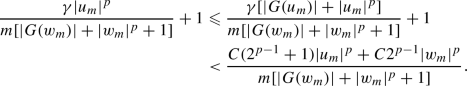
• If $\{u_m\}_m$ is unbounded, passing to a subsequence we have $|G(u_m)|\leqslant \gamma |u_m|^p$. So,

  

  By continuity of G, we have that $\{G(u_m+w_m)\}_m$ is bounded and therefore

  $$\begin{aligned} 1\leqslant \frac{\gamma |G(u_m)|}{m[|G(w_m)|+|w_m|^p+1]}+1 <\frac{|G(u_m+w_m)|}{m[|G(w_m)|+|w_m|^p+1]}\xrightarrow {m\rightarrow +\infty }0, \end{aligned}$$

  which is a contradiction.

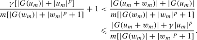
• If $\{|u_m|\}_m$ is bounded, there is $K>0$ such that $|G(u_m\,{+}\,w_m)|,|G(u_m)|\leqslant K$. Therefore

  $$\begin{aligned} 1\leqslant \frac{\gamma [|G(u_m)|+|u_m|^p]}{m[|G(w_m)|+|w_m|^p+1]}+1 <\frac{|G(u_m+w_m)|+|G(u_m)|}{m[|G(w_m)|+|w_m|^p+1]}\leqslant \frac{2K}{m}\rightarrow 0, \end{aligned}$$

  which is a contradiction. $\square$

In our case $n=5$, $d=3$, $p=6$, $\alpha =1$ and

(6)

Taking into account Lemma 2.4 it is easy to show that $g(q)=\nabla G(q)$ satisfies all conditions of Theorem 2.2. Moreover, it is easy to see that it also satisfies (4). Thus we have proved:

Corollary 2.5

Let $a,b,c\in {\mathbb {R}}$ with $a>0$ and $c<0$, then there exists a least energy solution ${\overline{q}}$ in $H^1({\mathbb {R}}^3;{\mathbb {R}}^5)$ for the system

Moreover, ${\overline{q}}$ decays exponentially as $|x|\rightarrow +\infty$.

2.2 Least energy solution as a saddle point

Let us recall the functional related to our model:

(7)

We assumed $a>0$ and $c<0$. This choice of signs for the parameters gives J a particular structure: since $c<0$, the functional is unbounded from below; however, the sign of a implies that J is positive near the zero. Such information suggests existence of a saddle point for the functional.

Definition 2.6

Let X be a Hilbert space and $J:X\rightarrow {\mathbb {R}}$ be a differentiable function, then we say that $\{q_n\}_n\subseteq X$ is a Palais–Smale sequence if $\{J(q_n)\}_n$ is bounded and $J^\prime (q_n)\rightarrow 0$ in $X^*$ as $n\rightarrow \infty$.

We say that $J:X\rightarrow {\mathbb {R}}$ satisfies the Palais–Smale condition (P.S.) when, for each Palais–Smale sequence, there is a convergent subsequence in X.

Theorem 2.7

(Mountain Pass Theorem [22]) Let X be a Hilbert space and $J\in C^1(X)$ be such that:

• J satisfies P.S.;

• $J(0)=0$ and there exist $\rho ,\alpha >0$ and $e\in X$ such that

  • if $\Vert q\Vert =\rho$ then $J(q)\geqslant \alpha$;

  • $\Vert e\Vert >\rho$ and $J(e)<0$;

then, for a fixed , the quantity

is a critical value of J in X.

Remark 2.8

Thanks to the geometric hypotheses of the theorem, it is easy to see that any critical point related to M is not 0.

It is not difficult to check that our J(q) belongs to $C^1(H^1({\mathbb {R}}^d;{\mathbb {R}}^n))$ and that it satisfies the geometric hypotheses of the Mountain Pass Theorem. Conversely, it is difficult to prove the P.S. condition is fulfilled. For this reason we use the Mountain Pass Theorem for J restricted to the space $H^1_{\mathrm{rad}}({\mathbb {R}}^d;{\mathbb {R}}^n)$: this set is weakly closed in $H^1({\mathbb {R}}^d;{\mathbb {R}}^n)$, in particular it is a Hilbert space. Moreover, its elements satisfy the following proposition:

Proposition 2.9

Given $r\in \bigl (2,\frac{2d}{d-2}\bigr )$ with $d\geqslant 3$, then $H^1_{\mathrm{rad}}({\mathbb {R}}^d;{\mathbb {R}}^n)\hookrightarrow L^r({\mathbb {R}}^d;{\mathbb {R}}^n)$ is a compact embedding.

Its proof follows from [21, Lemma 1].

Proposition 2.10

The function $J:H^1_{\mathrm{rad}}({\mathbb {R}}^3;{\mathbb {R}}^5)\rightarrow {\mathbb {R}}$ from (7) with $a>0$ and $c<0$ has a critical point ${\overline{q}}\ne 0$.

Proof

Let us denote and

which is equivalent to .

The idea is to show that J satisfies the hypotheses of the Mountain Pass Theorem. Firstly, we verify the geometric hypotheses:

• Obviously, $J(0)=0$.

• Let $\rho >0$ and q be such that $\Vert q\Vert _{H^1_*}=\rho$.

  

  Then, by Sobolev embeddings, there is $K>0$ such that

  $$\begin{aligned} J(q)\geqslant \rho ^2-K\Vert q\Vert _{H^1_*}^3-K\Vert q\Vert _{H^1_*}^4=\rho ^2(1-K\rho -K\rho ^2). \end{aligned}$$

  Therefore, we can find $\rho$ sufficiently small and $\alpha >0$ such that $J(q)\geqslant \alpha$ for any $\Vert q\Vert _{H^1_*}=\rho$.

• Fix ${\overline{q}}\in X$ different from 0 and let for $\lambda >0$.

  $$\begin{aligned} J(q_\lambda )&\lesssim \Vert \nabla q_\lambda \Vert _{L^2}^2+a\Vert q_\lambda \Vert _{L^2}^2 +|b|\Vert q_\lambda \Vert _{L^3}^3+c\Vert q_\lambda \Vert _{L^4}^4 \\&=\lambda ^2\Vert \nabla \, {\overline{q}}\Vert _{L^2}^2+a\lambda ^2\Vert {\overline{q}}\Vert _{L^2}^2 +\lambda ^3|b|\Vert {\overline{q}}\Vert _{L^3}^3+c\lambda ^4\Vert {\overline{q}}\Vert _{L^4}^4. \end{aligned}$$

  Therefore, since $c<0$, $J(q_\lambda )\rightarrow -\infty$ as $\lambda \rightarrow +\infty$, so we can choose $e=q_\lambda$ with $\lambda \gg 1$.

Now let us show that J satisfies the P.S. condition: let $\{q^k\}_k\subseteq X$ be a Palais–Smale sequence, that is

$$\begin{aligned} \left\{ \begin{aligned}&{}-2\Delta q^k-\Delta q_1^ke_2-\Delta q_2^ke_1+\nabla _qF(q^k)=dJ(q^k)\rightarrow 0\quad \text {in}\;\; X^*; \\&\biggl |\int |\nabla q^k|^2+\nabla q^k_1\nabla q^k_2+F(q^k)\,dx\biggr |\leqslant K \quad \text {for all}\;\; k\in {\mathbb {N}}. \end{aligned}\right. \end{aligned}$$

We recall that, for all $v\in X$, $\Vert dJ(q^k)[v]\Vert \leqslant \delta _k\Vert v\Vert \rightarrow 0$, where . In particular,

(8)

If we take $v=q^k$ , we get

Firstly we consider

Calculate $\mathrm{(U2)} + \frac{1}{2}\mathrm{(U1)}$:

One can check that

with

Notice that

Thanks to this, we get

(9)

Now, consider

Calculate $\mathrm{(L1)}-2\mathrm{(L2)}$:

(10)

Combining (9) and (10), we get

We have

Since $c<0$, we have

therefore,

$$\begin{aligned} \Vert q^k\Vert _{H^1_*}^2\leqslant 4\delta _k\Vert q^k\Vert _{H^1_*}+6K. \end{aligned}$$

So $\{q^k\}_k$ is bounded in X. Passing to a subsequence, we can suppose $q^k\rightharpoonup {\overline{q}}$ in X.

Now let us show the strong convergence. Take $v=q^k-{\overline{q}}$ in (8), then

Denote

It is clear that $q^k_a-{\overline{q}}_a=(q^k-{\overline{q}})_a$, so

$$\begin{aligned} dJ(q^k)[q^k-{\overline{q}}]-I_k=\Vert q^k-{\overline{q}}\Vert ^2_{H^1_*}+\int bq^k_b(q^k-{\overline{q}})+c|Q(q^k)|^2q_a^k(q^k-{\overline{q}})\,dx. \end{aligned}$$

We notice that $I_k=2\langle {\overline{q}},q^k-{\overline{q}}\rangle _{H^1_*}$ so, by weak convergence, $I_k\rightarrow 0$. We are then in the following situation:

$$\begin{aligned} \Vert q^k-{\overline{q}}\Vert ^2_{H^1_*}+\int b q^k_b(q^k-{\overline{q}})+c|Q(q^k)|^2q_a^k(q^k-{\overline{q}})dx\rightarrow 0. \end{aligned}$$

We need to show that the last two terms tend to 0 as $k\rightarrow +\infty$. Thanks to Proposition 2.9, we can suppose also that $q^k\rightarrow {\overline{q}}$ in $L^4({\mathbb {R}}^3;{\mathbb {R}}^5)$. Then

$$\begin{aligned} \left\{ \begin{aligned}&\biggl |\int |Q(q^k)|^2q_a^k(q^k-{\overline{q}})\,dx\biggr |\lesssim \int |q^k|^3|q^k-{\overline{q}}|\,dx\leqslant \Vert q^k\Vert _{L^4}^3\Vert q^k-{\overline{q}}\Vert _{L^4}; \\&\biggl |\int q^k_b(q^k-{\overline{q}})\,dx\biggr |\lesssim \int |q^k|^2|q^k-{\overline{q}}|\,dx\leqslant \Vert q^k\Vert _{L^{8/3}}^2\Vert q^k-{\overline{q}}\Vert _{L^4}. \end{aligned}\right. \end{aligned}$$

Since ${8}/{3}\in [2,6]$ and $\{q^k\}_k$ is bounded in $H^1({\mathbb {R}}^3;{\mathbb {R}}^5)$, we are done. $\square$

The least energy solution ${\overline{q}}$ built in the Sect. 2.1 can be seen as a saddle point of the functional J(q), similarly to the one given by the Mountain Pass Theorem:

where

In fact, with the same techniques as in [14], one can prove

Theorem 2.11

Let $J:H^1({\mathbb {R}}^d;{\mathbb {R}}^n)\rightarrow {\mathbb {R}}$ with $d\geqslant 3$ and $n\geqslant 2$ be defined as

$$\begin{aligned} J(q)=\int |\nabla q|^2+\alpha \nabla q_1\nabla q_2-G(q)\,dx, \end{aligned}$$

where $\alpha \in [0,1]$; let G satisfy the hypotheses of Theorem 2.2 and condition (4). Let us also suppose that there exists $\rho _0>0$ such that

where

let be the least energy solution built in Theorem 2.2, then

Proof

We give a sketch of the proof:

Step 1: Since G satisfies condition (4), thanks to Theorem 2.3 we have that ${\overline{q}}\in H^1({\mathbb {R}}^d;{\mathbb {R}}^n)$. Let

with $L>0$. It can be seen that, for L sufficiently small, $J(\gamma (1))<0$, so $\gamma \in \Gamma$. On the other hand, thanks to Step 4 in the proof of Theorem 2.2, we have

$$\begin{aligned} \frac{d}{dt}\,J(\gamma (t))&=\frac{d-2}{L^{d-2}}\,t^{d-3}\Vert \nabla {\overline{q}}\Vert _*^2-\frac{d}{L^d}\,t^{d-1}\int G({\overline{q}})\,dx\\&=\frac{d-2}{L^{d-2}}\,t^{d-3}\Vert \nabla {\overline{q}}\Vert _*^2\,\biggl (1-\frac{t^2}{L^2} \biggr ). \end{aligned}$$

So $J({\overline{q}})=J(\gamma (L))=\max _{t\in [0,1]}J(\gamma (t))$. In particular, $J({\overline{q}})\geqslant M$, where

Step 2: Let

One can check that

is invertible as .

Step 3: It can be seen from the proof of Theorem 2.2 that ${\overline{q}}=\phi (q)$ with q such that

On the other hand, ${\overline{q}}\in H^1({\mathbb {R}}^d;{\mathbb {R}}^n)$, so $q\in H^1({\mathbb {R}}^d;{\mathbb {R}}^n)$ and we also proved that $\int G(q)\,dx=1$. Then

Thanks to the previous step,

Step 4: For any $\gamma \in \Gamma$, we have that . Let

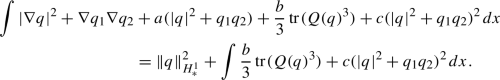
We notice that $S(q)=dJ(q)-2\Vert \nabla q\Vert _*^2$. For any $\gamma \in \Gamma$ we then have

$$\begin{aligned} S(\gamma (0))=0,\quad S(\gamma (1))\leqslant d J(\gamma (1))<0. \end{aligned}$$

It is clear that $S\in C(H^1({\mathbb {R}}^d;{\mathbb {R}}^n))$, so we can find $t_0\in [0,1]$ such that $S(\gamma (t_0))=0$. We also know by hypothesis that

$$\begin{aligned} 0<\Vert q\Vert _{H^1_*}\leqslant \rho _0\,\Longrightarrow \, S(q)>0. \end{aligned}$$

Therefore, $\Vert \gamma (t_0)\Vert >\rho _0$. In particular, .

Thus

$\square$

Just to conclude, we note that

Proposition 2.12

If G(q) is continuous and satisfies

$$\begin{aligned} \limsup _{|q|\rightarrow 0^+}\frac{G(q)}{|q|^2}\leqslant -\nu <0,\quad \limsup _{|q|\rightarrow +\infty }\frac{G(q)}{|q|^p}\leqslant 0, \end{aligned}$$

then there exists $\rho _0>0$ such that

$$\begin{aligned} 0<\Vert q\Vert _{H^1_*}\leqslant \rho _0\,\Longrightarrow \, S(q)>0. \end{aligned}$$

So our functional (7) satisfies also the additional hypothesis of Theorem 2.11.

3 Evolution equation

Consider the system

(11)

where $G(Q)=bQ^2+c|Q|^{p-1}Q$ with $a>0$, $b,c\in {\mathbb {R}}$ and $p\in (1,5)$.

Let us recall that by Duhamel’s formula any solution Q of (11) satisfies the following equality:

$$\begin{aligned} Q(t,x)=e^{(\Delta -a) t}Q_0(x)+\int _0^te^{(\Delta -a)(t-\tau )}G(Q(\tau ,x))\,d\tau , \end{aligned}$$

where with .

Proposition 3.1

Let $t>0$ and $1\leqslant r\leqslant q\leqslant \infty$, then

$$\begin{aligned} \Vert e^{(\Delta -a) t}f\Vert _{L^q_x}\lesssim t^{-\frac{n}{2}\bigl (\frac{1}{r}-\frac{1}{q}\bigr )}e^{-at}\Vert f\Vert _{L^r}. \end{aligned}$$

The proof follows using the well-known estimates on $K_t$ and the Young inequality.

3.1 Strichartz estimates

Consider the problem

(12)

with $Q_0$ and F taken in a suitable space to be chosen later.

Our aim is to obtain certain estimates in the space $L^q({\mathbb {R}}^+;L^r({\mathbb {R}}^3;S_0(3,{\mathbb {R}})))$ for $q,r\in (1,+\infty )$. We will use the norm

Theorem 3.2

Let $I\subseteq {\mathbb {R}}^+$ , then for $q\in [1,+\infty )$ and $r\in (1,\infty )$ the dual of $L^q_t(I;L^r_x)$ is isometric to $L^{q^\prime }_t(I;L^{r^\prime }_x)$ with the duality pair

In particular, when $q>1$, these spaces are reflexive.

The proof follows from [10, Theorems 8.20.3 and 8.20.5, pp. 602–607].

Let us consider the following spacial class of exponents:

Definition 3.3

Let $\sigma >0$, then (q, r) is said to be a $\sigma$-admissible couple if $q,r\geqslant 2$, $(q,r,\sigma )\ne (2,\infty ,1)$ and

If the equality holds, the couple is called strictly $\sigma$-admissible. Moreover, when $\sigma >1$, the couple $\bigl (2,\frac{2\sigma }{\sigma -1}\bigr )$ is called the endpoint.

Thanks to [15, Theorem 1.2] and the embedding theorems for $H^s$ with $s>0$ (which can be found in [5, pp. 153–154]) we get

Proposition 3.4

Let $a\geqslant 0$, then

$$\begin{aligned} \bigl \Vert e^{(\Delta -a)t}f\bigr \Vert _{L^q_tL^r_x}\lesssim \Vert f\Vert _{H^s} \end{aligned}$$

where $q,r\geqslant 2$, $s\in \bigl [0,\frac{n}{2}-\frac{2}{q}\bigr )$ and

Let us obtain an estimate for the term $\int _0^t e^{(\Delta -a)(t-\tau )}F(\tau ,x)\,d\tau$.

Proposition 3.5

Let $\lambda >0$ and $I,J\subseteq {\mathbb {R}}^+$ be such that $l(I)=l(J)=\lambda$ and $d(I,J)\approx \lambda$, then, for all $r,{\widetilde{r}}\in [2,+\infty ]$ and $q,{\widetilde{q}}\in [1,+\infty ]$,

(13)

where

Proof

Firstly is defined only on I but, preserving the notation we can suppose that it is defined on ${\mathbb {R}}^+$ with support on I. If $\sup J<\inf I$, then the left-hand side of (13) is equal to zero, since $\tau \not \in I$. In this case the inequality is obvious.

Let us suppose now that $\sup I<\inf J$. Then

$$\begin{aligned}&\biggl \Vert \int _0^te^{\Delta (t-\tau )}F(\tau )\,d\tau \biggr \Vert _{L^r_x}\\&\quad \leqslant \int _0^t \bigl \Vert e^{\Delta (t-\tau )}F(\tau )\bigr \Vert _{L^r_x}d\tau \lesssim \int _0^t\frac{1}{|t-\tau |^{\frac{n}{2}\bigl (\frac{1}{{\tilde{r}}^\prime }-\frac{1}{r}\bigr )}} \,\Vert F(\tau )\Vert _{L^{{\tilde{r}}^\prime }_x}\,d\tau \end{aligned}$$

which follows from Proposition 3.1.

since $I\subseteq [0,t]$ for $t\in J$. If ${\widetilde{q}}<+\infty$ by the Hölder inequality

By hypothesis, $d(I,J)=\lambda$, $t\in J$ and $\tau \in I$, then $|t-\tau |\geqslant \lambda$ so

where we have used that $|I|=|J|=\lambda$. For ${\widetilde{q}}=\infty$ it is easier:

$\square$

Theorem 3.6

For any $r,{\widetilde{r}}\in [2,+\infty )$ and $q,{\widetilde{q}}\in (1,+\infty )$ such that

$$\begin{aligned} \frac{1}{q}+\frac{1}{{\widetilde{q}}}=\frac{n}{2}\, \biggl (\frac{1}{{\widetilde{r}}^\prime }-\frac{1}{r}\biggr ),\quad \frac{1}{q}+\frac{1}{{\widetilde{q}}}<1 \end{aligned}$$

we have the following inequality:

$$\begin{aligned} \biggl \Vert \int _0^te^{\Delta (t-\tau )}F(\tau )\,d\tau \biggr \Vert _{L^q_tL^r_x}\lesssim \Vert F\Vert _{L^{{\tilde{q}}^\prime }_tL^{{\tilde{r}}^\prime }_x} . \end{aligned}$$

Proof

If we denote

by duality we get

Let us define the bilinear form

To show that

$$\begin{aligned} |B(F,G)|\lesssim \Vert F\Vert _{L^{{\tilde{q}}^\prime }_tL^{{\tilde{r}}^\prime }_x}\, \Vert G\Vert _{L^{q^\prime }_tL^{r^\prime }_x}, \end{aligned}$$

it is useful to rewrite the operator B as

Then we conclude following the proof of [11, Theorem 1.4]. $\square$

Before passing to the main theorem of this section, let us remark that

Let us also assume the condition of Proposition 3.4 (in the case $s=0$) holds:

$$\begin{aligned} \frac{1}{q}+\frac{n}{2r}=\frac{n}{4}\,\Longleftrightarrow \, \frac{1}{q}=\frac{n}{2}\,\biggl (\frac{1}{2}-\frac{1}{r}\biggr ). \end{aligned}$$

Then the condition on the indices in Theorem 3.6 becomes

$$\begin{aligned} \frac{1}{{\widetilde{q}}}=\frac{n}{2}\, \biggl (\frac{1}{{\widetilde{r}}^\prime }-\frac{1}{r}\biggr )-\frac{1}{q} =\frac{n}{2}\,\biggl (\frac{1}{{\widetilde{r}}^\prime }-\frac{1}{2}\biggr ) =\frac{n}{2}\,\biggl (\frac{1}{2}-\frac{1}{{\widetilde{r}}}\biggr ). \end{aligned}$$

This means that (q, r) and $({\widetilde{q}},{\widetilde{r}})$ are strictly $\frac{n}{2}$-admissible.

Theorem 3.7

Let $a\geqslant 0$, $n\geqslant 3$, $r,{\widetilde{r}},q,{\widetilde{q}}\in [2,+\infty )$ be such that (q, r) and $({\widetilde{q}},{\widetilde{r}})$ are strictly $\frac{n}{2}$-admissible and such that $\frac{1}{r}+\frac{1}{{\widetilde{r}}}>\frac{n-2}{n}$. If and $Q_0\in L^2({\mathbb {R}}^n;S_0(3,{\mathbb {R}}))$, then there is a solution Q of (12) such that

The proof follows from Proposition 3.4, Theorem 3.6 and the above remarks.

For simplicity, in what follows we shall take $n=3$. If $Q_0\in H^s({\mathbb {R}}^3;S_0(3,{\mathbb {R}}))$, then we have more freedom in the choice of couples:

Certainly, if $Q_0\in H^s({\mathbb {R}}^3;S_0(3,{\mathbb {R}}))$, then $Q_0\in H^l({\mathbb {R}}^3;S_0(3,{\mathbb {R}}))$ for every $l\in [0,s]$. If we ignore the condition $\frac{1}{r}+\frac{1}{{\widetilde{r}}}>\frac{1}{3}$, the two areas representing the admissible couples are the following:

excluding the points on the axes. Precisely, these two sets are defined as

Corollary 3.8

Let $a\geqslant 0$, $s\geqslant 0$, and be such that $\frac{1}{{\widetilde{r}}}+\frac{1}{r}>\frac{1}{3}$. If and $Q_0\in H^s({\mathbb {R}}^3;S_0(3,{\mathbb {R}}))$, then there is a solution Q of (12) such that

Remark 3.9

The theorem holds also when one of the couples is an endpoint.

Remark 3.10

The theorem holds also when we work with $J=[0,T]$ instead of ${\mathbb {R}}^+$: we only need to switch with u and with F, getting

The constant C does not depend on T.

Another important result is the following smoothing inequality.

Proposition 3.11

Let $s\geqslant 0$ and $a,T>0$ be constants, let $Q_0\in H^s({\mathbb {R}}^3;S_0(3,{\mathbb {R}}))$ and $F\in L^2([0,T];H^{s-1}({\mathbb {R}}^3;S_0(3,{\mathbb {R}})))$, let Q be a solution of (12), then Q satisfies

$$\begin{aligned} \Vert Q\Vert _{L^\infty _tH^s_x}^2+\Vert Q\Vert _{L^2_tH^{s+1}_x}^2\lesssim \Vert Q_0\Vert _{H^s}^2+\Vert F\Vert _{L^2_tH^{s-1}_x}^2. \end{aligned}$$

Proof

Firstly we prove the case $s=0$: let us multiply (12) by Q(t, x):

$$\begin{aligned} \frac{1}{2}\,\frac{d}{dt}\,\Vert Q(t)\Vert _{L^2_x}^2+\Vert \nabla Q(t)\Vert _{L^2_x}^2+a\Vert Q(t)\Vert _{L^2_x}^2\leqslant \bigl |\langle F(t),Q(t)\rangle _{L^2_x}\bigr |. \end{aligned}$$

Since $a>0$, it is clear that $\Vert Q(t)\Vert _{H^1_x}\simeq \Vert (a\mathrm{Id}-\Delta )^{1/2}Q(t)\Vert _{L^2_x}$ for any $t\geqslant 0$. Then we have

$$\begin{aligned} \begin{aligned} \frac{1}{2}\,\frac{d}{dt}\,\Vert Q(t)\Vert _{L^2_x}^2+\Vert Q(t)\Vert _{H^1_x}^2&\lesssim \frac{1}{2}\,\frac{d}{dt}\, \Vert Q(t)\Vert _{L^2_x}^2+\bigl \Vert (a-\Delta )^{{1/2}}u(t)\bigr \Vert _{L^2_x}^2\\&\lesssim \bigl |\langle F(t),Q(t)\rangle _{L^2_x}\bigr |. \end{aligned} \end{aligned}$$

By the Plancherel identity, we have

$$\begin{aligned} \bigl |\langle F(t),Q(t)\rangle _{L^2_x}\bigr |&=\bigl |\langle {\widehat{F}}(t),{\widehat{Q}}(t)\rangle _{L^2_\xi }\bigr |\\&=\bigl |\bigl \langle (a+|\xi |^2)^{-{1/2}}{\widehat{F}}(t),(a+|\xi |^2)^{1/2}{\widehat{Q}}(t)\bigr \rangle _{L^2_\xi }\bigr |\\&\leqslant C_\varepsilon \bigl \Vert (a+|\xi |^2)^{-{1/2}}{\widehat{F}}(t)\bigr \Vert _{H^{-1}_\xi }^2 +\varepsilon \bigl \Vert (a+|\xi |^2)^{1/2}{\widehat{Q}}(t)\bigr \Vert _{L^2_\xi }^2\\&\leqslant \widetilde{C_\varepsilon }\Vert F(t)\Vert _{H^{-1}_x}^2+C_2\varepsilon \Vert Q(t)\Vert _{H^1_x}^2. \end{aligned}$$

If we take $\varepsilon <{1}/{C_2}$, then

$$\begin{aligned} \frac{1}{2}\,\frac{d}{dt}\,\Vert Q(t)\Vert _{L^2_x}^2+\Vert Q(t)\Vert _{H^1_x}^2\lesssim \Vert F(t)\Vert _{H^{-1}_x}^2 \end{aligned}$$

and taking the integral from 0 to T we achieve the result.

For the case $s>0$ we only need to apply this result to $(\mathrm{Id}-\Delta )^{s/2}Q$.$\square$

3.2 Local existence of the solutions

We consider the following spaces:

where

In the following, for simplicity, we omit the index s. With respect to the previous theorems, we assume $r,{\widetilde{r}}<6$ so that the condition ${1}/{r}+{1}/{{\widetilde{r}}}> {1}/{3}$ is automatically satisfied. In this case, thanks to Proposition 3.4 and Theorem 3.6 we obtain

Moreover, Remark 3.10 tells us that this inequality holds for any $T>0$.

Lemma 3.12

Let $s\in \bigl [0,\frac{3}{2}\bigr )$ and $p\in \bigl (\frac{5}{3},\min \bigl \{5,\frac{7}{3-2s}\bigr \}\bigr )$, then there are $\varepsilon _0,\delta _0>0$ such that for all $\varepsilon \in (0,\varepsilon _0)$, $\delta \in (0,\delta _0)$ there exist

such that $l_1+{\widetilde{l}}_1,l_2+{\widetilde{l}}_2\in \bigl [\frac{5}{3},5\bigr )$ and

All the couples, the parameters $\gamma _1,\gamma _2$ and $l_1,{\widetilde{l}}_1,l_2,{\widetilde{l}}_2$ depend on the choice of $\varepsilon$ and $\delta$.

The proof is technical and follows from several uses of interpolation and Hölder inequalities.

Remark 3.13

If we want to capture all the powers $p\in \bigl [\frac{5}{3},5\bigr )$, it is necessary to assume that $s\geqslant \frac{4}{5}$.

We are finally ready to prove the existence and uniqueness of the solution in $S_T$.

Theorem 3.14

Let $s\geqslant 0$, $p\in \bigl [\frac{5}{3},5\bigr )$ be such that $p<\frac{7}{3-2s}$, let $a\geqslant 0$ and $b,c\in {\mathbb {R}}$. If $Q_0\in H^s({\mathbb {R}}^3;S_0(3,{\mathbb {R}}))$ with for some $R>0$, then there is $T=T(R)>0$ such that there exists a unique $Q\in B(0,R)\subseteq S_T$ which satisfies

Proof

The idea of the proof is to apply the Banach Fixed Point Theorem to the operator

on the ball B(0, R) of the Banach space

for T and R sufficiently small (the couples $(q_i,k_i)$ are the ones of Lemma 3.12 for both the powers in G(Q)). In particular, for any , we have the inequality

Therefore, if T and R are sufficiently small, then there exists a unique solution of the Cauchy problem.

Let us see that $Q\in S_T$: let , define for ${\widetilde{T}}$ to be defined. Thanks to what we have already proved we get

On the other hand,

So, exactly as before, it can be proved that there exists a unique fixed point for K. Moreover the choice of ${\widetilde{T}}$ is the same as before: it depends only on some global constants (thanks to Remark 3.10) and on R, which can be taken as before. In conclusion, we can choose ${\widetilde{T}}=T$. On the other hand, , in particular the R-balls of the two spaces share the same inclusion. So, by uniqueness of the fixed point in the greater ball, $Q={\widetilde{Q}}$ and therefore $Q\in L^q_t([0,T];L^r_x)$. Certainly, this argument can be repeated for all , so $Q\in B(0,R)\subseteq S_T$.$\square$

Before finishing this section, let us present some regularity results.

Proposition 3.15

If $Q\in S_T$ is a solution of

$$\begin{aligned} \left\{ \begin{aligned}&(\partial _t-\Delta +a)Q(t,x)=G(Q), \\&Q(0,x)=Q_0(x)\in H^1({\mathbb {R}}^3;S_0(3,{\mathbb {R}})) \end{aligned}\right. \end{aligned}$$

(14)

for $p\!\in \!\bigl [\frac{5}{3},5\bigr )$, then $Q\!\in \! L^\infty ([0,T];H^1({\mathbb {R}}^3;S_0(3,{\mathbb {R}})))\cap L^2([0,T];H^2({\mathbb {R}}^3;S_0(3,{\mathbb {R}})))$.

Proof

Thanks to Proposition 3.11, we have

$$\begin{aligned} \Vert Q\Vert _{L^\infty _tH^1_x}^2+\Vert Q\Vert _{L^2_tH^2_x}^2&\lesssim \Vert Q_0\Vert _{H^1}^2+\Vert G(Q)\Vert _{L^2_tL^2_x}^2\\&\leqslant \Vert Q_0\Vert _{H^1}^2+\Vert Q\Vert _{L^4_tL^4_x}^2+\Vert Q\Vert _{L^{2p}_tL^{2p}_x}^2. \end{aligned}$$

Therefore, for a fixed $p\in \bigl [\frac{5}{3},5\bigr )$, we only need to see that :

$$\begin{aligned} \frac{1}{2p}\leqslant \frac{3}{2}\,\biggl (\frac{1}{2}-\frac{1}{2p}\biggr )\,\Longleftrightarrow \, p\geqslant \frac{5}{3},\quad \frac{1}{2p}\geqslant \frac{3}{2}\,\biggl (\frac{1}{2}-\frac{1}{2p}\biggr )-\frac{1}{2}\,\Longleftrightarrow \, p\leqslant 5. \end{aligned}$$

$\square$

Proposition 3.16

If $Q\in S_T$ is a solution of (14) for $p\in \bigl [\frac{5}{3},5\bigr )$, then $Q\in C([0,T];H^1({\mathbb {R}}^3;S_0(3,{\mathbb {R}})))$.

Proof

Let us take $s,t\geqslant 0$.

$$\begin{aligned} Q(t,x)&-Q(s,x)\\&= \int _s^t e^{(\Delta -a)(t-\tau )}G(Q(\tau ,x))\,d\tau \\&\qquad \qquad \quad +\bigl (e^{(\Delta -a)(t-s)}-\mathrm{Id}\bigr )\,\biggl [\int _0^s e^{(\Delta -a)(s-\tau )}G(Q(\tau ,x))\,d\tau \biggr ]. \end{aligned}$$

Let us see what happens to the first term when $s\rightarrow t$: thanks to Proposition 3.1, it is easy to see that for any $p\in \bigl [\frac{5}{3},5\bigr )$ and $r\leqslant \frac{6}{p}$,

Let us evaluate the part related with the $L^2$-norm of the gradient:

Thanks to Proposition 3.15, we know that $Q\in L^\infty ([0,T];L^q({\mathbb {R}}^3;S_0(3,{\mathbb {R}})))$ and that $\nabla Q\in L^2([0,T];L^q({\mathbb {R}}^3;S_0(3,{\mathbb {R}})))$ for any $q\in [2,6]$. So, if we take $r=\frac{6}{p}$, $\alpha =\frac{6}{r(p-1)}$ and $\beta =\frac{6}{6-r(p-1)}$, we get

As for the second term, by similar calculations we have

with $r=\frac{6}{p}$. In particular, this term is bounded for $s\rightarrow t$. On the other hand, it is easy to see that $e^{(\Delta -a)\varepsilon }\rightarrow \mathrm{Id}$ as $\varepsilon \rightarrow 0+$ as a map from $H^1({\mathbb {R}}^3;S_0(3,{\mathbb {R}}))$ to itself. $\square$

3.3 Global existence and decay for $t\rightarrow +\infty$

Let us show that any solution of (11) does not blow up in a finite time when the data are “small”.

Proposition 3.17

If $Q\in C([0,T); H^1({\mathbb {R}}^3;S_0(3,{\mathbb {R}})))$ is a solution of

$$\begin{aligned} \left\{ \begin{aligned}&(\partial _t -\Delta +a)Q=bQ^2+c|Q|^{p-1}Q,\\&Q(0,x)=Q_0(x)\in H^1({\mathbb {R}}^3;S_0(3,{\mathbb {R}})), \end{aligned}\right. \end{aligned}$$

(15)

where $1<p<5$ and $a,b,c\in {\mathbb {R}}$, then

(16)

It can be gained multiplying the equation by Q.

It can be seen that, for sufficiently small, the local solution exists globally. However we can do better: we only need to require that $\Vert Q_0\Vert _{L^2}$ is small.

Proposition 3.18

If $Q(t,x)\in C([0,T);H^1({\mathbb {R}}^3;S_0(3,{\mathbb {R}})))$ is a solution of (15), where $\frac{5}{3}<p<\frac{7}{3}$, $a>0$, $b,c\in {\mathbb {R}}$ and , then there is $\varepsilon$ sufficiently small such that and for $t\geqslant 0$.

Proof

We start from equality (16), which can be rewritten as

If we denote and , then we have

for all $\delta >0$, where we have used that $\frac{3(p-1)}{4}<1$ for $p<\frac{7}{3}$. Therefore, if we take $\delta ^4+\delta ^\frac{4}{7-3p}=1$, then

$$\begin{aligned} f^\prime (t)\leqslant \overline{C_1}e^{-4at}f(t)^3 +\overline{C_2}e^{-\frac{4a(p-1)}{7-3p}t}f(t)^\frac{5-p}{7-3p}. \end{aligned}$$

By comparison, we have that $f(t)\leqslant y(t)$ for y(t) which satisfies

$$\begin{aligned} \left\{ \begin{aligned}&y^\prime (t)=\overline{C_1}e^{-4at}y(t)^3 +\overline{C_2}e^{-\frac{4a(p-1)}{7-3p}t}y(t)^\frac{5-p}{7-3p},\\&y(0)=f(0)=\Vert Q_0\Vert ^2. \end{aligned}\right. \end{aligned}$$

Let us show that there exists $\varepsilon$ sufficiently small such that y(t) is uniformly bounded on $t\in {\mathbb {R}}^+$ . Let us start with the case of just one non-linearity:

$$\begin{aligned} \left\{ \begin{aligned}&y^\prime (t)={\overline{C}}e^{-B t}y(t)^A, \\&y(0)=\Vert Q_0\Vert ^2. \end{aligned}\right. \end{aligned}$$

With $A>1$ and $B,{\overline{C}}>0$, it is easy to prove that

$$\begin{aligned} y(t)=\frac{1}{(A-1)\bigl (\frac{{\overline{C}}}{B}\, e^{-Bt}-\gamma \bigr )} \end{aligned}$$

where

If we take $\Vert Q_0\Vert _{L^2}\leqslant \varepsilon$ sufficiently small such that $\gamma < 0$, then $y(t)\leqslant -\frac{1}{(A-1)\gamma }$ for all $t\geqslant 0$.

Let us return to the case of two non-linearities. If, by contradiction, y(t) were unbounded, then, for any $\varepsilon >0$, there would exist $T_\varepsilon >0$ such that

$$\begin{aligned} y(t)\leqslant 1\quad \text {for all}\;\; t<T_\varepsilon ,\;\; y(T_\varepsilon )=1. \end{aligned}$$

If we call , and , then $y(t)\leqslant w(t)$ with w(t) solution of

$$\begin{aligned} \left\{ \begin{aligned}&w^\prime (t)={\overline{C}}e^{-B t}w(t)^A ,\\&w(0)=\Vert Q_0\Vert ^2. \end{aligned}\right. \end{aligned}$$

We already know that $w(t)\leqslant -\frac{1}{(A-1)\gamma }$ and we can take $\varepsilon$ sufficiently small so that $\gamma <-\frac{1}{A-1}$. In this case $w(t)< 1$ for any $t\in {\mathbb {R}}^+$ . In particular, $y(T_\varepsilon )\leqslant w(T_\varepsilon )<1$ which gives us a contradiction.$\square$

Corollary 3.19

If $Q(t,x)\in C([0,T);H^1({\mathbb {R}}^3;S_0(3,{\mathbb {R}})))$ is a solution of (15), where $\frac{5}{3}<p<\frac{7}{3}$, $a>0$, $b,c\in {\mathbb {R}}$ and , then there is $\varepsilon$ sufficiently small such that for any $t\geqslant 0$.

Proof

Let us take $V\in H^1({\mathbb {R}}^3;S_0(3,{\mathbb {R}}))$ such that $Q(t,x)=e^{-at}V(t,x)$. The function V satisfies

$$\begin{aligned} \partial _t V-\Delta V=be^{-at}V^2+ce^{-(p-1)at}|V|^{p-1}V. \end{aligned}$$

If we multiply this equation by $\partial _t V$, we get

(17)

By Proposition 3.17 we have that so, integrating (17), we get

For $\beta _1,\beta _2<2$, since $x^\beta \leqslant 1+x^2$ for any $\beta \leqslant 2$ and for any $x\geqslant 0$, we get

Finally, we apply the Grönwall inequality and obtain

$$\begin{aligned} \Vert \nabla V(\tau )\Vert \leqslant {\widetilde{C}}e^{\int _0^t e^{-a\tau }+e^{-a(p-1)\tau }d\tau }\lesssim 1\quad \text {for all}\;\; t\geqslant 0. \end{aligned}$$

We are done, since $\Vert \nabla Q(t)\Vert _{L^2_x}=e^{-at}\Vert \nabla V(t)\Vert _{L^2_x}$.$\square$

References

Andrienko, D.: Introduction to liquid crystals. Journal of Molecular Liquids 267, 520–541 (2018)
Ball, J.: The Mathematics of Liquid Crystals. Cambridge CCA Course (2012). https://people.maths.ox.ac.uk/ball/Teaching/cambridge.pdf
Ball, J.M., Majumdar, A.: Nematic liquid crystals: From Maier-Saupe to a continuum theory. Molecular Crystals and Liquid Crystals 525(1), 1–11 (2010)
Ball, J.M., Zarnescu, A.D.: Orientability and energy minimization in liquid crystal model. Arch. Ration. Mech. Anal. 202(2), 493–535 (2011)
Bergh, J., Löfström, J.: Interpolation Spaces. Grundlehren der Mathematischen Wissenschaften, vol. 223. Springer, Berlin (1976)
Brezis, H., Lieb, E.H.: Minimum action solutions of some vector field equations. Comm. Math. Phys. 97(1), 97–113 (1984)
Cavaterra, C., Rocca, E., Wu, H., Xu, X.: Global strong solutions of the full Navier-Stokes and\( Q\)-tensor system for nematic liquid crystal flows in two dimensions. SIAM J. Math. Anal. 48(2), 1368–1399 (2016)
Dai, M., Feireisl, E., Rocca, E., Schimperna, G., Schonbek, M.E.: On asymptotic isotropy for a hydrodynamic model of liquid crystals. Asymptot. Anal. 97(3–4), 189–210 (2016)
De Gennes, P.G., Prost, J.: The Physics of Liquid Crystals. Oxford University Press, New York (1993)
Edwards, R.E.: Functional Analysis. Holt, Rinehart and Winston, New York (1965)
Foschi, D.: Inhomogeneous Strichartz estimates. Hyperbolic. Differ. Equ. 2(1), 1–24 (2005)
Georgiev, V., Barbera, D.: Least energy solutions for a model of liquid crystals. In: Seventh International Conference on New Trends in the Applications of Differential Equations in Sciences (NTADES 2020). AIP Conference Proceedings 2321, Art. No. 030001 (2021)
Iyer, G., Xu, X., Zarnescu, A.D.: Dynamic cubic instability in a 2d \(Q\)-tensor model for liquid crystals. Math. Models Methods Appl. Sci. 25(8), 1477–1517 (2015)
Jeanjean, L., Tanaka, K.: A remark on least energy solution in \({\mathbb{R} }^N\). Amer. Math. Soc. 131(8), 2399–2408 (2002)
Keel, M., Tao, T.: Endpoint Strichartz estimates. Amer. J. Math. 120(5), 955–980 (1998)
Mottram, N.J., Newton, C.J.P.: Introduction to \(Q\)-tensor theory (2014). arXiv:1409.3542
Paicu, M., Zarnescu, A.D.: Global existence and regularity for the full coupled Navier-Stokes and \(Q\)-tensor system. SIAM J. Math. Anal. 43(5), 2009–2049 (2011)
Paicu, M., Zarnescu, A.: Energy dissipation and regularity for a coupled Navier-Stokes and \(Q\)-tensor system. Arch. Ration. Mech. Anal. 203(1), 45–67 (2012)
Schonbek, M., Shibata, Y.: Global well-posedness and decay for a \(Q\)-tensor model of incompressible nematic liquid crystals in \({\mathbb{R} }^N\). J. Differential Equations 266(6), 3034–3065 (2019)
Schonbek, M., Shibata, Y.: On the global well-posedness of strong dynamics of incompressible nematic liquid crystals in \({\mathbb{R} }^N\). J. Evol. Equ. 17(1), 537–550 (2017)
Strauss, W.A.: Existence of solitary waves in higher dimensions. Comm. Math. Phys. 55(2), 149–162 (1977)
Struwe, M.: Variational Methods: Applications to Nonlinear Partial Differential Equations and Hamiltonian Systems. Ergebnisse der Mathematik und ihrer Grenzgebiete, vol. 34. 2nd edn. Springer, Berlin (1996)
Virga, E.G.: Variational Theories for Liquid Crystals. Applied Mathematics and Mathematical Computation, vol. 8. Chapman & Hall, London (1994)
Wu, H., Xu, X., Zarnescu, A.: Dynamics and flow effects in the Beris-Edwards system modeling nematic liquid crystals. Arch. Ration. Mech. Anal. 231(2), 1217–1267 (2019)
Zarnescu, A.: Mathematical problems of nematic liquid crystals: between dynamical and stationary problems. Philos. Trans. Roy. Soc. A 379(2201), Art. No. 20200432 (2021)
Acknowledgements
We are grateful to the anonymous referee for remarks and suggestions which improved the presentation.
Funding
Open access funding provided by Università di Pisa within the CRUI-CARE Agreement.
Author information
Authors and Affiliations
Corresponding author
Additional information
Publisher's Note
Springer Nature remains neutral with regard to jurisdictional claims in published maps and institutional affiliations.
Daniele Barbera is supported in part by INDAM — Gruppo Nazionale per l’Analisi Matematica, la Probabilità e le loro Applicazioni. Vladimir Georgiev is partially supported by Project 2017 “Problemi stazionari e di evoluzione nelle equazioni di campo nonlineari” of INDAM, GNAMPA — Gruppo Nazionale per l’Analisi Matematica, la Probabilità e le loro Applicazioni, by Institute of Mathematics and Informatics, Bulgarian Academy of Sciences, by Top Global University Project, Waseda University, the Project PRA 2018 49 of University of Pisa and by the project PRIN 2020XB3EFL funded by the Italian Ministry of Universities and Research.
Rights and permissions
Open Access This article is licensed under a Creative Commons Attribution 4.0 International License, which permits use, sharing, adaptation, distribution and reproduction in any medium or format, as long as you give appropriate credit to the original author(s) and the source, provide a link to the Creative Commons licence, and indicate if changes were made. The images or other third party material in this article are included in the article’s Creative Commons licence, unless indicated otherwise in a credit line to the material. If material is not included in the article’s Creative Commons licence and your intended use is not permitted by statutory regulation or exceeds the permitted use, you will need to obtain permission directly from the copyright holder. To view a copy of this licence, visit http://creativecommons.org/licenses/by/4.0/.
About this article
Cite this article
Barbera, D., Georgiev, V. On standing waves and gradient-flow for the Landau–De Gennes model of nematic liquid crystals. European Journal of Mathematics 8, 672–699 (2022). https://doi.org/10.1007/s40879-022-00537-5
Received:
Revised:
Accepted:
Published:
Issue Date:
DOI: https://doi.org/10.1007/s40879-022-00537-5