Cyclopermutohedron: geometry and topology

Abstract

The face poset of the permutohedron realizes the combinatorics of linearly ordered partitions of the set . Similarly, the cyclopermutohedron is a virtual polytope that realizes the combinatorics of cyclically ordered partitions of the set . The cyclopermutohedron was introduced by the second author by motivations coming from configuration spaces of polygonal linkages. In the paper we prove two facts: (a) the volume of the cyclopermutohedron equals zero, and (b) the homology groups $H_k$ for $k=0,\ldots ,n-2$ of the face poset of the cyclopermutohedron are non-zero free abelian groups. We also present a short formula for their ranks.

1 Introduction

The standard permutohedron $\mathrm{\Pi }_n$ (see [7]) is defined as the convex hull of all points in $\mathbb {R}^n$ that are obtained by permuting the coordinates of the point $(1, 2, \dots , n)$. It has the following properties:

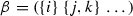
Here and in the sequel, by a refinement we mean an order preserving refinement. For instance, the label refines the label but does not refine .

• (II) $\mathrm{\Pi }_n$ is an -dimensional polytope.

• (III) $\mathrm{\Pi }_n$ is a zonotope, that is, the Minkowski sum of line segments $q_{ij}$, whose defining vectors are , where are the standard orthonormal basis vectors.

By analogy, we replace the linear order by cyclic order and build up the following regular¹ cell complex $\textit{CP}_{n+1}$ [3], see Fig. 1.

• (I) Assume that $n>2$. For $k=0, \dots , n-2$, the k-dimensional cells (k-cells, for short) of the complex $\textit{CP}_{n+1}$ are labeled by (all possible) cyclically ordered partitions of the set into $n-k+1$ non-empty parts.

• (II) A (closed) cell F contains a cell $F'$ whenever the label of $F'$ refines the label of F. Here we again mean order-preserving refinement.

The cyclopermutohedron $\mathscr {CP}_{n+1}$ is a virtual polytope whose face poset is combinatorially isomorphic to complex $\textit{CP}_{n+1}$. More details will be given in Sect. 2.1; for a complete presentation see [3].

Fig. 1

These are labels of two cells whose dimensions are 3 and 4. The first cell is a face of the second one

In the paper we study geometry and topology of the cyclopermutohedron. Before we formulate the main result some explanation is needed. The cyclopermutohedron is a virtual polytope, that is, the Minkowski difference of two convex polytopes. A detailed discussion on virtual polytopes can be found in the survey [4]. One of the messages of the survey is that virtual polytopes inherit almost all properties and structures of convex polytopes: the volume (together with its polynomiality property), normal fan, face poset, etc. However, virtual polytopes do not inherit the convexity property and therefore may appear as counter-intuitive: (a) The volume of a virtual polytope, although well-defined, can be negative, see [2, 4]. The volume also can turn to zero, even if the virtual polytope does not degenerate. (b) The face poset of a virtual polytope is also well-defined. However, it is not necessarily isomorphic to a combinatorial sphere. So one can expect non-zero homologies in all dimensions.

The main results of the paper are:

Theorem 1.1

The volume of the cyclopermutohedron $\mathscr {CP}_{n+1}$ equals zero.

Fig. 2

Left The face poset of $\mathscr {CP}_{4}$. We indicate labels of all vertices and labels of two edges. Middle The cyclopermutohedron $\mathscr {CP}_{4}$ represented by a closed polygon, the limit of the polygon depicted on the right

Theorem 1.2

The homology groups of the face poset of the cyclopermutohedron $\mathscr {CP}_{n+1}$ are free abelian groups. Their ranks are:

Let us understand the meaning of these theorems for the toy example $n=3$, that is, for $\mathscr {CP}_{4}$. The complex $\textit{CP}_{4}$ (and therefore, the face poset of the cyclopermutohedron) is the graph with six vertices and twelve edges, see Fig. 2, left. Its Betti numbers are 1 and 7.

The cyclopermutohedron $\mathscr {CP}_{4}$ (computed in [3]) can be represented by a closed polygon, whereas its area (that is, two-dimensional volume) equals the integral of the winding number against the Lebesgue measure (see [4]). In other words, in this case the volume equals “sum of areas of six small triangles minus the area of the hexagon” in Fig. 2 (middle), which is zero.

We use the following methods: (a) Proof of Theorem 1.1 is based on the polynomiality of the volume combined with the theory of Abel polynomials. The proof resembles the volume computation of the standard permutohedron, which reduces to counting of spanning trees. (b) Theorem 1.2 is proven via discrete Morse theory by Forman [1]. In a sense, it is a simplification of the approach of [5] where a perfect discrete Morse function on the moduli space of a polygonal linkage was constructed.

One of motivations for considering the cyclopermutohedron comes from polygonal linkages. A polygonal n-linkage is a generic sequence of positive numbers $L=(l_1, \dots , l_n)$. It should be interpreted as a collection of rigid bars of lengths $l_i$ joined consecutively in a chain by revolving joints.

The space M(L) of all planar configurations modulo orientation preserving isometries of $\mathbb {R}^2$ is the moduli space, or configuration space, of the linkage L. It is proven (see [3]) that M(L) admits the structure of a regular cell complex whose description literally repeats the combinatorics of the cyclopermutohedron except when all partitions are admissible, that is, the total length of any part does not exceed the total length of the rest. Such a partition has at least three parts. Consequently, for any n-linkage L, the cell complex combinatorially embeds in the face lattice of the cyclopermutohedron $\mathscr {CP}_n$.

2 Theoretical backgrounds and toolboxes

2.1 Virtual polytopes [4]

Virtual polytopes appeared in the literature as useful geometrization of Minkowski differences of convex polytopes; below we give just a brief sketch.

A convex polytope is the convex hull of a finite, non-empty point set in the Euclidean space $\mathbb {R}^n$. The Minkowski addition turns the set of all convex polytopes $\mathscr {P}^+$ into a commutative semigroup whose unit element is the single-point polytope .

Definition 2.1

The group $\mathscr {P}$ of virtual polytopes is the Grothendieck group associated to the semigroup $\mathscr {P}^+$. The elements of $\mathscr {P}$ are called virtual polytopes.

More instructively, $\mathscr {P}$ can be explained as follows.

• A virtual polytope is a formal difference $K- L$ of convex polytopes.

• Two such expressions $K_1 - L_1$ and $K_2 - L_2$ are identified, whenever $K_1 + L_2 = K_2 + L_1$ as convex polytopes.

• The group operation is defined by

  $$\begin{aligned} (K_1 - L_1) + (K_2 - L_2) = (K_1 + K_2)- (L_1 + L_2). \end{aligned}$$

2.2 Cyclopermutohedron [3]

Assuming that are standard basis vectors in $\mathbb {R}^n$, define the points

and the following two families of line segments: , $i<j$, and . We also need the point $e=(1, 1, \dots , 1)\in \mathbb {R}^{n}$. The cyclopermutohedron is a virtual polytope defined as the Minkowski sum:

Throughout the paper the sign “$\bigoplus$” denotes the Minkowski sum, whereas the sign “$\sum$” is reserved for the sum of numbers.

The cyclopermutohedron lies in the hyperplane $x_1+\cdots +x_n=n(n+1)/2$, so its dimension is $n-1$. Therefore, by its volume we mean the -volume.

The face poset of $\mathscr {CP}_{n+1}$ is isomorphic to the complex $\textit{CP}_{n+1}$ (defined in Sect. 1) [3].

2.3 Abel polynomials and rooted forests [6]

A rooted forest is a disjoint union of trees, where each of the trees has one marked vertex. The Abel polynomials form a sequence of polynomials, where the n-th term is defined by

$$\begin{aligned} A_{n,a}(x)=x(x-an)^{n-1}. \end{aligned}$$

A special case of Abel polynomials with counts rooted labeled forests. Namely, if is the n-th Abel polynomial, then

where $t_{n,k}$ is the number of forests on n labeled vertices consisting of k rooted trees.

2.4 Discrete Morse theory on a regular cell complex [1]

Assume we have a regular cell complex X. By $\alpha ^p, \beta ^p$ we denote its p-dimensional cells, or p-cells, for short. A discrete vector field on X is a set of pairs $(\alpha ^p,\beta ^{p+1})$ such that:

• each cell of the complex participates in at most one pair,

• in each pair, the cell $\alpha ^p$ is a facet of the cell $\beta ^{p+1}$.

Given a discrete vector field, a gradient path is a sequence of cells

$$\begin{aligned} \beta _0^{p+1},\quad \alpha _1^p,\quad \beta _1^{p+1}, \quad \alpha _2^p,\quad \beta _2^{p+1} ,\quad \dots ,\quad \alpha _m^p,\quad \beta _m^{p+1},\quad \alpha _{m+1}^p, \end{aligned}$$

which satisfies the conditions:

• each $(\alpha _i^p, \beta _i^{p+1})$ is a pair;

• $\alpha _i^p$ is a facet of $\beta _{i-1}^{p+1}$;

• $\alpha _i \ne \alpha _{i+1}$ for any i.

A path is closed if $\alpha _{m+1}^p$ is paired with $\beta _0^{p+1}$. A discrete Morse function is a discrete vector field without closed paths.

Assuming that a discrete Morse function is fixed, the critical cells are those cells of the complex that are not paired. The Morse index of a critical cell is its dimension. The Morse inequality says that we cannot avoid them completely. However, our goal is to minimize their number.

The discrete Morse function theory allows to compute homology groups. Fix an orientation for each of cells of complex and introduce the free abelian groups $\mathscr {M}_k(X,\mathbb {Z})$ whose generators bijectively correspond to critical cells of index k. These groups are incorporated in the chain complex called the Morse complex associated with X

$$\begin{aligned} \cdots \rightarrow \mathscr {M}_k(X,\mathbb {Z}) \rightarrow \mathscr {M}_{k-1}(X,\mathbb {Z})\rightarrow \cdots , \end{aligned}$$

where the boundary operators ${\partial _k}$ are defined by

where $\alpha$ ranges over all -dimensional cells, and is the number of gradient paths from $\beta ^k$ to $\alpha ^{k-1}$. Each gradient path is counted with a sign $\pm 1$, depending on whether the orientation of $\beta ^k$ induces the already fixed orientation on $\alpha ^{k-1}$, or the opposite one. With this boundary operators the above complex computes the homology groups of X:

3 Volume of cyclopermutohedron equals zero

As we have already mentioned, the notion of volume extends nicely from convex polytopes to virtual polytopes. We explain here the meaning of the volume of a virtual zonotope.

Assume we have a convex zonotope $Z\subset \mathbb {R}^n$, that is, the Minkowski sum of some linear segments $\{s_i\}_{i=1}^m$:

For each subset such that $|I| = n$, denote by $Z_I$ the elementary parallelepiped, or the brick spanned by n segments , provided that the defining vectors of the segments are linearly independent. In other words, the brick equals the Minkowski sum

It is known that Z can be partitioned into the union of all such $Z_I$, which implies immediately

where $S_I$ is the matrix composed of defining vectors of the segments from I. Now take positive $\lambda _1, \dots , \lambda _m$ and sum up the dilated segments $\lambda _is_i$. Clearly, we have

For fixed $s_i$, we get a polynomial in $\lambda _i$, which counts not only the volume of the convex zonotope (which originates from positive $\lambda _i$), but also the volume of a virtual zonotope, which originates from any real $\lambda _i$, including negative ones, see [4]. So, one can use the above formula as the definition of the volume of a virtual zonotope.

Lemma 3.1

Let $E=E_n$ be the set of edges of the complete graph $K_n$. The -volume of the cyclopermutohedron can be computed by the formula:

Here I ranges over subsets of E, whereas M ranges over subsets of . The matrix under determinant is composed of defining vectors of the segments $q_{ij}$ and $r_k$, and also of the vector $e=(1, 1, \dots , 1, 1)$.

Proof

The dimension of the cyclopermutohedron equals $n - 1$. That is, we deal with -volume, which reduces to the n-volume by adding $e=(1, 1, \dots , 1, 1)$ and dividing by $|e|=\sqrt{n}$.$\square$

Now we are ready to prove Theorem 1.1. Keeping in mind Lemma 3.1, let us first fix sets I and M with $|I|+|M|=n-1$, and compute one single summand .

If $M=\varnothing$, the determinant equals 1 iff the set I gives a tree; otherwise it is zero.

Assume now that M is not empty.

We wish to proceed in a similar way, that is, add columns containing the unique non-zero entry 1 to other columns chosen in an appropriate way. To explain this reduction let us give two technical definitions.

Definition 3.2

A decorated forest $F=(G,M)$ is a graph without cycles on n labeled vertices together with a set of marked vertices such that the following conditions hold:

• (i) number of marked vertices |M| $+$ number of edges |I| equals $n-1$;

• (ii) each connected component of G has at most one marked vertex.

Immediate observations are: (a) Each decorated forest has exactly one connected component with no vertices marked. We call it a free tree. Denote by N(F) the number of vertices of the free tree. (b) Each decorated forest is a disjoint union of the free tree and some rooted trees. The number of rooted trees equals |M|. (c) Each decorated forest F yields a collection of , whose above determinant $(\star )$ we denote by for short. For instance, for the first decorated forest in Fig. 3, we have $N(F)=2$, $|M|= 1$.

Now we define the reduction of a decorated forest (see Fig. 3 for example). It goes as follows. Assume we have a decorated forest. Take a marked vertex i and an incident edge (ij). Remove the edge and mark the vertex j. Repeat until is possible. Roughly speaking, a marked vertex i kills the edge (ij) and generates a new marked vertex j.

Fig. 3

Reduction process for a forest with $N(F)=2$, $|M|(F)= 1$. Grey balls denote the marked vertices

An obvious observation is

Lemma 3.3

• The free tree does not change during the reduction.

• The reduction brings us to a decorated forest with a unique free tree. All other trees are one-vertex trees, and all these vertices are marked.

• The reduction can be shortened: take the connected components one by one and do the following. If a connected component has a marked vertex, eliminate all its edges and mark all its vertices. Otherwise leave the connected component as it is.

• The reduction does not depend on the order of marked vertices we deal with.

Before we proceed with the proof of Theorem 1.1, we prove the following result.

Lemma 3.4

• (i) For each decorated forest F, .

• (ii) If a collection does not come from a decorated forest, that is, violates condition (ii) from Definition 3.2, then .

Proof

(i) For a decorated forest, we manipulate with columns according to the reduction process. We arrive at a matrix which (up to a permutation of the columns and up to a sign) is

$$\begin{aligned} \left( \begin{matrix} A &{} O &{}1\\ O &{} E &{}1\\ \end{matrix} \right) . \end{aligned}$$

Here A is the matrix corresponding to the free tree, E is the unit matrix, and the very last column is e. Its determinant equals 1.

(ii) If the collection of vectors does not yield a decorated forest, that is, there are two marked vertices on one connected component, the analogous reduction gives a zero column.$\square$

Basing on Lemmata 3.4 and 3.1, we conclude

where the sum extends over all decorated forests F on n vertices. (Recall that M(F) is the set of marked vertices, N(F) is the number of vertices of the free tree.)

Next, we group the forests by the number $N=N(F)$ and write

where the second sum ranges over all rooted forests on $n-N$ labeled vertices, is the number of connected components.

Let us explain this in more details: (a) N ranges from 1 to n. We choose N vertices in $\left( {\begin{array}{c}n\\ N\end{array}}\right)$ different ways and place a tree on these vertices in $N^{N-2}$ ways. (b) On the rest of vertices we place a rooted forest.

Since $t_{n-N,k}$ is the number of forests on $n-N$ labeled vertices of k rooted trees, we write

Section 2.3 gives us $\sum _{k = 0}^{n} t_{n,k}x^{k} = A_{n}(x)$, where is the Abel polynomial.

Setting , we get

Thus $(\star \star )$ converts to

Applying the definition of , we get

Introduce the following polynomial:

for which we have . Set also

We clearly have $p(x) = p_{n-2}(x)$. Besides, $(1+x)^{n - k}$ divides $p_{k}(x)$, which implies $Q_{n} = 0$. The proof is complete.

4 Homologies of the face poset of cyclopermutohedron

Since the face poset of $\mathscr {CP}_{n+1}$ is isomorphic to the complex $\textit{CP}_{n+1}$ (defined in Sect. 1), in this section we shall work with the latter complex.

Let us make the following conventions that are illustrated in Fig. 1. First recall that k-cells of the complex are labeled by (all possible) cyclically ordered partitions of the set into $n-k+1$ non-empty parts, so the number of parts is at least 3.

• Instead of the “cell of the complex $\textit{CP}_{n+1}$ labeled by $\alpha$” we say for short the “cell $\alpha$”.

• For a cell $\alpha$ the -set is the set in the partition containing the entry $n+1$.

• We represent a cyclically ordered partition $\alpha$ as a linearly ordered partition of the same set by cutting the circle right after the -set. For example, the labels depicted in Fig. 1 we write as and . In particular, the vertices of the complex $\textit{CP}_{n+1}$ are labeled by (all possible) permutations of the set ending with the entry $n+1$. Therefore we have a map : the removal of from the label gives an element of the symmetric group $S_{n}$.

• For a cell $\alpha$ we denote by $|\alpha |$ the number of parts in the partition. Recall that we always have $|\alpha |\geqslant 3$.

• For and a set we write $i<I$ whenever $j\in I$ implies $i<j$.

• A singleton is a one-element set.

4.1 Discrete Morse function on the complex $\textit{CP}_{n+1}$

Let us introduce a discrete Morse function on cells of the complex $\textit{CP}_{n+1}$. It is going to be a perfect Morse function, and therefore will give us the homology groups directly.

Step 1. We pair together two cells

iff $n+1\notin I$.

We proceed for all $2 \leqslant k< n$, assuming that the k-th step is

Step k. We pair together two cells

iff the following holds:

• $\alpha$ and $\beta$ were not paired at any of the previous steps.

• $n+1\notin I$.

• $k<I$.

Example 4.1

The cell is paired with on the second step. The cell is paired with on the fourth step. The cell is not paired.

It is convenient to reformulate the above as an algorithm for finding a pair for a given cell $\alpha$ (if such a pair exists).

Pair search algorithm. Take a cell $\alpha$.

• I. We call an entry forward-movable in $\alpha$ if

  • $\alpha$ consists of more than three subsets;

  • k forms a singleton in $\alpha$;

  • the singleton is followed by a set I such that $k<I$ and $n+1\notin I$.

• II. We call an entry backward-movable in $\alpha$ if

  • the entry k lies in $\alpha$ in a non-singleton set J, such that $n+1\notin J$;

  • ;

  • one of the following conditions holds:

    • the set J is preceded by a non-singleton set;

    • the set J is preceded by a singleton with $m > k$;

    • the set J is preceded by a set containing $n+1$.

In this notation, the algorithm looks as follows:

• I. If a cell $\alpha$ has no movable entries, $\alpha$ is not paired.

• II. Assuming that a cell $\alpha$ has movable entries, take the minimal movable (either forward or backward) entry k in $\alpha$. Then the cell $\alpha$ is paired with a cell that is formed from $\alpha$ by moving k either forward inside the next set, or backward out of the set containing k, according to the k-th step of pairing algorithm.

Lemma 4.2

The above pairing is a discrete Morse function.

Proof

The conditions “each cell of the complex participates in at most one pair” and “in each pair, the cell $\alpha ^p$ is a facet of the cell $\beta ^{p+1}$” hold automatically. The “no closed paths” condition follows from the observation that no two entries interchange their order during a path more than once. $\square$

Lemma 4.3

The critical cells of the above defined Morse function are exactly all cells of the following two types:

Type 1. Cells labeled by , where is a string of singletons coming in decreasing order.

Type 2. Cells labeled by , where $i<I$.

Indeed, these are exactly all labels that do not have movable entries.

Example 4.4

is a critical cell of type 1, is a critical cell of type 2, is a critical cell of type 2.

Lemma 4.5

For the discrete Morse function there are exactly

$$\begin{aligned} 2^n+\frac{n^2-3n-2}{2} \end{aligned}$$

critical cells of dimension $n-2$, and exactly

$$\begin{aligned} \left( {\begin{array}{c}n\\ k\end{array}}\right) \end{aligned}$$

critical cells of dimension k for all $0\leqslant k < n-2$.

Lemma 4.6

The boundary operators of the Morse complex vanish.

Theorem 1.2 follows from the above two lemmata and Sect. 2.4.

The proof of Lemma 4.6 is contained in the next section. The detailed proof is somewhat technical, but the idea is simple: we show that for each pair of critical cells $\alpha$ and $\beta$ either there are no gradient paths leading from $\beta$ to $\alpha$, or there are exactly two paths coming with different orientations.

5 Proof of Lemma 4.6

5.1 Gradient paths

Let us describe the gradient paths connecting critical cells $\beta ^{p+1}$ and $\alpha ^{p}$.

Lemma 5.1

There are no critical gradient paths that end at critical cells of type 2.

Indeed, critical cells of type 2 have the maximal possible dimension.

Lemma 5.2

The three following cases describe all gradient paths joining critical cells:

• 1. Let and be two cells of type 1. Then there are two gradient paths from $\beta$ to $\alpha$ iff $\heartsuit = \spadesuit \cup \{k\}$ for some k.

• 2. Let and be cells of type 2 and 1 respectively. Then there are two gradient paths from $\beta$ to $\alpha$.

• 3. Let and be cells of type 2 and 1 respectively. Then there are two gradient paths from $\beta$ to $\alpha$ iff consists of three singletons, and two of them are and .

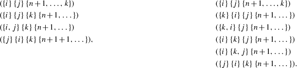
We start with examples:

• For and the two paths are:

  

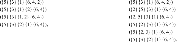
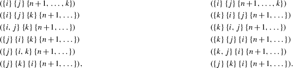
• For , where $i<j<k$, the two paths are:

  

• For and there are three possible cases:

  Case 1. For $k<i<j$ the two paths from $\beta$ to $\alpha$ are:

  

  Case 2. For $i<k<j$ the two paths are:

  

  Case 3. For $i<j<k$ the two paths are:

  

Now prove the lemma.

Proof

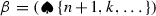
Case 1. Suppose there is a path from $\beta$ to $\alpha$. Then , therefore, . Since no entry joins the -set during the path, we have $\heartsuit = \spadesuit \cup \{k\}$ for some k.

Now we have , . The existent gradient paths come from a simple case analysis. The other two cases are proved in a similar way.$\square$

5.2 Canonical orientations of cells

Recall that two vertices of $\textit{CP}_{n+1}$ are joined by an edge whenever their labels differ on a permutation of two neighbor entries. Such vertices we will call neighbors. For a cell $\alpha = (I_{1} I_{2} \dots I_{l})$, a vertex $V \in \alpha$ has exactly neighbors that belong to $\alpha$. The latter are called $\alpha$-neighbors of V. For every $V \in \alpha$ we order $\alpha$-neighbors of V: we get the first neighbor of V by interchanging the first² two entries of V that belong to the same set $I_i$, the second neighbor we get by interchanging the second two entries of V that belong to the same $I_i$, etc. This ordering defines the orientation of the cell $\alpha$ related to the vertex V. Here we explore the following observation: cells of the complex are combinatorially isomorphic to the product of permutohedra, and therefore can be realized as some convex polytopes. More precisely, a cell labeled by $(I_1, \dots , I_m)$ is combinatorially isomorphic to . To fix an orientation on a polytope, it suffices to fix an order on all vertices that are neighbors of a fixed vertex.

The principal vertex of the cell $\alpha$ is the vertex with the label $(\widehat{I_{1}}, \widehat{I_{2}}, \dots , \widehat{I_{l}})$, where $\widehat{I_{j}}$ is a partition of the set $I_{j}$ into singletons coming in increasing order. The orientation of the cell $\alpha$ related to its principal vertex is called the canonical orientation of the cell $\alpha$.

Example 5.3

(i) For the cell and its vertex $\alpha$-neighbors of V are ordered as follows: , ,

(ii) For the cell the principal vertex is .

For a cell $\alpha$ and its vertex , the permutation $\sigma _{V,\alpha } \in S_{n}$ is defined by

Lemma 5.4

In the above notation the orientation of a cell $\alpha$ related to a vertex V equals .

5.3 Boundary operators vanish

Now we are ready to prove Lemma 4.6. As we have seen, each pair of critical cells is connected either by no paths or by exactly two paths. To show that in the latter case paths come with different orientations (this is exactly what the lemma states) we analyze elementary steps in two auxiliary lemmata.

Assume we have a gradient path

$$\begin{aligned} \beta ^{p+1}_0,\quad \alpha ^p_1,\quad \beta ^{p+1}_1,\quad \alpha ^p_2,\quad \beta ^{p+1}_2,\quad \dots ,\quad \alpha ^p_k,\quad \beta ^{p+1}_k,\quad \alpha ^p_{k+1}, \end{aligned}$$

with $\beta ^{p+1}_0$ and $\alpha ^p_{k+1}$ critical. By definition, two consecutive $\beta ^{p+1}_i$ and $\beta ^{p+1}_{i+1}$ share a facet $\alpha ^p_i$. To compute the sign of this path, we compare canonical orientations of $\beta ^{p+1}_i$ and $\beta ^{p+1}_{i+1}$. We also need to compare orientations of cells $\beta ^{p+1}_k$ and $\alpha ^p_{k+1}$. We are especially interested in the first steps of paths (which can be of both types).

For a cell $\beta$ and , denote by $N (\beta , k)$ (respectively, $M (\beta , k)$) the number of entries in the -set of $\beta$ which are bigger (respectively, smaller) than k.

Lemma 5.5

(first steps) Now suppose we have two critical cells $\beta$ and $\alpha$ connected by two paths.³ Then exactly one of the first steps in these paths has disagreement in canonical orientations. More precisely, we have the following.

• (I)

  • (a) For $k>i$ canonical orientations of cells and agree iff $N (\beta , k)$ is odd.

  • (b) For $k<i$ canonical orientations of cells and agree iff $M (\beta , k)$ and have different parity.

  • (c) For $k>i$ canonical orientations of cells and agree iff $N (\beta , k)$ is odd.

  • (d) For $k<i$ canonical orientations of cells and agree iff $M (\beta , k)$ and have different parity.

• (II)

  • (a) For $i<j<k$ canonical orientations of cells and 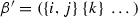always disagree.

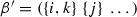  • (b) For $i<j<k$ canonical orientations of cells and always agree.

• (III)

  • (a) For $i<j$ canonical orientations of cells and agree iff $N (\beta , k)$ is odd.

  • (b) For $i<j$ canonical orientations of cells and agree iff $M (\beta , k)$ and have different parity.

Proof

We give the proof of some cases.

(I.a) Note that . We have

There are exactly $N(\beta , k)$ elementary transpositions that turn to . So, by Lemma 5.4, the orientation associated with in $\beta$ is positive iff $N(\beta , k)$ is even. Observe also that orientation at for cells $\beta$ and $\beta '$ are opposite.

(I.b) Take the vertex . It belongs to the cell $\beta$. differs from by $M(\beta ,k)$ elementary transpositions. Therefore, by Lemma 5.4, the orientation, associated with in $\beta$ is positive iff $M(\beta , k)$ is even.

Now consider the orientation of $\beta '$. If we denote the $\beta$-neighbors of by

$$\begin{aligned} A_1,A_2,\dots , A_{\dim (\beta )}, \end{aligned}$$

then its $\beta '$-neighbors are

$$\begin{aligned} A', A_1, A_2, \dots , A_{\dim (\beta )-1} , \end{aligned}$$

where . It is easy to see that the orientations, associated with A in $\beta '$ and $\beta$, agree iff is even.

(II.a) . differs from by one elementary transposition. If we denote $\beta$-neighbors of by

$$\begin{aligned} A_1, A_2, \dots , A_{\dim (\beta )}, \end{aligned}$$

then its $\beta '$-neighbors are

$$\begin{aligned} A', A_2, \dots , A_{\dim (\beta )-1}, \end{aligned}$$

where .

All other cases are treated analogously.$\square$

The following lemma is proved in a similar way as Lemma 5.5.

Lemma 5.6

(intermediate and last steps) Assume that two critical cells $\beta$ and $\alpha$ are connected by two paths. At all steps of gradient (except for the first steps) paths canonical orientations always agree.

Now the proof of Lemma 4.6 comes from the two above lemmata.

6 Concluding remark

The anonymous referee gave the following valuable comment: it is known that the permutohedron is a space-filling polytope, and therefore can be considered as a fundamental domain of some group of translations. The factor space (that is, the permutohedron with identified by parallel translation opposite faces) is a torus, and its natural cell structure is that of $\textit{CP}_{n+1}$ plus a number of -dimensional cells. The latter correspond to facets of the permutohedron, that is, to partitions of into two parts. Therefore, homologies of $\textit{CP}_{n+1}$ in dimensions up to $n-3$ coincide with those of a torus, and the top homology can be extracted from Euler characteristic.

We also add that another way to see the ambient torus of the complex $\textit{CP}_{n+1}$ comes from the cell decomposition of the configuration space of a robot arm. However, we leave the detailed discussion for further papers.

References

Forman, R.: Morse theory for cell complexes. Adv. Math. 134, 90–145 (1998)
Martinez-Maure, Y.: De nouvelles inégalités géométriques pour les hérissons. Arch. Math. (Basel) 72(6), 444–453 (1999)
Panina, GYu.: Cyclopermutohedron. Proc. Steklov Inst. Math. 288(1), 132–144 (2015)
Panina, G.Yu., Streinu, I.: Virtual polytopes. Uspekhi Mat. Nauk 70(6)(426), 139–202 (2015) (in Russian)
Panina, G., Zhukova, A.: Discrete Morse theory for moduli spaces of flexible polygons, or solitaire game on the circle (2015). arXiv:1504.05139
Sagan, B.E.: A note on Abel polynomials and rooted labeled forests. Discrete Math. 44(3), 293–298 (1983)
Ziegler, G.M.: Lectures on Polytopes. Graduate Texts in Mathematics, vol. 152. Springer, New York (1995)
Acknowledgments
We are indebted to the anonymous referee for his/her clarifying remark.
Author information
Authors and Affiliations
Corresponding author
Additional information
The present research is supported by RFBR, research Project No. 15-01-02021. The first author is also supported by JSC “Gazprom Neft”. The third author is also supported in part by the Young Russian Mathematics Award.
Rights and permissions
About this article
Cite this article
Nekrasov, I., Panina, G. & Zhukova, A. Cyclopermutohedron: geometry and topology. European Journal of Mathematics 2, 835–852 (2016). https://doi.org/10.1007/s40879-016-0107-3
Received:
Revised:
Accepted:
Published:
Issue Date:
DOI: https://doi.org/10.1007/s40879-016-0107-3