
Abstract
Due to their heat/cool storage characteristics, thermostatically controlled loads (TCLs) play an important role in demand response programmers. However, modeling of the heat/cool storage characteristic of large numbers of TCLs is not simple. In this paper, the heat exchange power is adopted to calculate the power instead of the average power, and the relationship between the heat exchange power and energy storage is considered to develop an equivalent storage model, based on which the time-varying power constraints and the energy storage constraints are developed, to establish the overall day-ahead scheduling model. Finally, the proposed scheduling method is verified using the simulation results of a six-bus system.
1 Introduction
Recently, renewable energies, such as wind and solar energy, have garnered significant attention. However, due to the uncertainty and intermittency of these energies, their high penetration will bring about challenges for power grid scheduling [1, 2]. Demand response (DR) enables customers to participate in power system scheduling through price or incentive, and plays a more and more important role in shaving the peak load, restraining the fluctuation caused by new energy, and so on [3,4,5,6].
Thermostatically controlled loads (TCLs), such as air conditioning, refrigerators, and water heaters, are important DR resources. Further, TCLs have a great potential to participate in DR programmers, because even when they are suddenly shut down, the amount of heat/cool they store will last for a while, without causing much impact on customers [7].
In the scheduling of TCL participation, different methods have been proposed to deal with them [8,9,10,11]. In [8], in a commercial building containing the air conditioning system, the optimal meeting scheduling method is put forward to minimize the energy cost. In [9], a day-ahead scheduling model based on the self-adaptive TCL grouping method is proposed. Direct load control with the fuzzy adaptive imperialist competitive algorithm is adopted in [10] to schedule the air conditioner loads. Further, to satisfy the comfort of the customers, customer convenience is also taken into consideration in [9,10,11].
Recently, the heat/cool storage characteristics of TCLs have garnered increasing attention. The energy storage model is a good method to deal with these characteristics, and there have been several papers that propose energy storage models for TCLs [12,13,14,15,16,17]. Regarding the inverter air conditioner, a thermal battery model is established for the power dispatch model in [12]. To provide regulation service, a generalized battery model is proposed in [13], based on which, the improved battery model is established by considering heterogeneous parameters and the no-short-cycling requirement [14]. Further, the aggregate flexibility of TCLs based on the generalized battery model is further verified in [15]. The battery model usually contains the information of power constraints and energy storage constraints. The average power is used to calculate the charging and discharging power [16, 17], in which the time-varying characteristic of the average power is neglected, and the upper/lower limit of power is constant. In [13,14,15], although the heat exchange power is adopted instead of the average power, in the battery model, the upper/lower limit of power is still seen to be a constant by optimization.
Though effectiveness of the above models, the heat exchange power not only changes with the temperature, but also has a relationship with the aggregate energy storage, which will result in a time-varying upper/lower limit of power. However, these models either neglect this time-varying characteristic or this relationship between the power and energy storage.
To fill this research gap, this paper establishes an equivalent energy storage model for aggregated TCLs with heterogeneous parameters by introducing the heat exchange power instead of the average power, to reflect the time-varying characteristics. Further, the relationship between the heat exchange power and energy storage is established too. In this way, the upper/lower limit of power in the equivalent energy storage model is not a constant, but changes with time. Further, the scheduling can be more accurate.
The rest of this paper is organized as follows. Section 2 introduces the equivalent energy storage model, based on which the day-ahead scheduling of large numbers of TCLs is established in Section 3. The testing results are analyzed in Section 4 and the conclusions are drawn in Section 5.
2 Equivalent energy storage model
2.1 Equivalent thermal parameter model
Because the equivalent thermal parameter (ETP) model is simple and precise, it is always used to characterize the dynamics of an individual TCL. The first order equivalent thermal parameter model of one TCL is shown in Fig. 1.

The first-order equivalent thermal parameter model for one TCL
According to references [18,19,20], the ETP model of one TCL can be expressed as follows:
where Tin(t) is the inside air temperature at time t; Ta(t) is the ambient temperature at time t; R is the equivalent thermal resistance; C is the equivalent heat capacity; Q is the equivalent heat rate; Δt is the time step; and s(t) is the on/off state of a TCL at time t, defined as follows:
where s = 1 represents the “on” state and s = 0 represents the “off” state. When the user sets the temperature as Tset, through the compressor, the TCL will control the temperature within a range, namely (Tmin, Tmax) and Tmax = Tset + ε/2, Tmin = Tset − ε/2, where ε is the dead-band.
2.2 Equivalent energy storage model
As TCLs have heat/cool storage characteristics, the power can be equivalent to the charging and discharging power, and the storage of heat/cool can be equivalent to the energy storage. Then, the equivalent energy storage model can be established to characterize the aggregated dynamics.
The actual electric power of the ith TCL is Pe,i, obtained from:
where θ is the energy efficiency ratio.
Among all the parameters, the values of θ and Ta of each TCL are nearly the same; therefore, here we assume that all the θ and Ta are the same.
TCLs at runtime are periodically switched on and off, and their duty cycle equals the actual run time ton divided by the total time ton + toff. Then, the aggregated average power Pa,agg can be obtained as shown in (4).
where Pe,agg is the actual aggregated electric power, obtained from (5).
where Qave means the average value of Qi.
In [16, 17], Pa,agg is directly adopted to calculate the aggregate charging and discharging power Pc,agg of TCLs.
However, [16, 17] neglect the time-varying characteristic of Pa,agg. The temperature of TCLs changes with time; therefore, Pa,agg will change with the temperature. For this reason, constant Pa,agg is not suitable for obtaining Pc,agg.
To improve the accuracy of the modeling, the heat exchange power between TCLs and the outside is adopted to calculate Pc,agg in this paper. At time t, the heat exchange power Pex,i of ith TCL is shown in (8).
In (8), Pex,i shows the heat/cool loss rate of the TCLs, which changes with the temperature of the TCLs.
Assuming that a TCL is in refrigeration mode, Tmin can be seen as the zero point of energy storage. Then, at time t, the energy storage Ei(t) of ith TCL is shown as follows:
By eliminating the variable Tin,i according to (8) and (9), the relationship between Pex,i(t) and Ei(t) is obtained.
To characterize the aggregate dynamics of large numbers of TCLs, the easiest method is to model each individual TCL, and then the aggregate charging and discharging power can be superimposed by each individual TCL.
Assuming there are n TCLs, Pc,agg is shown in (11).
where Pex,agg is the aggregated heat exchange power.
Then, based on (10), the relationship between Pex,agg and Eagg can be obtained in (12), from which we can see that Pex,agg is time-varying, changing with Eagg.
where Eave, Cave, Rave and Tmin,ave are the average values; Eagg is the aggregated energy storage. Further,
Furthermore, TCLs have the characteristics of thermal energy storage, and the heat/cool variation quantity of large numbers of TCLs during ∆t can be expressed through the energy storage variation quantity ∆E, shown as follows.
According to (5), (12) and (16), the recursion formula between Eagg(t + 1) and Eagg(t) is obtained in (17).
Finally, based on (11)–(17), the equivalent energy storage model of large numbers of TCLs is established.
3 Day-ahead scheduling of model of large numbers of TCLs
The day-ahead scheduling model based on the equivalent energy storage model, which considers the Pc,agg constraint and Eagg constraint, is established in this section. To obtain the optimal cost-effectiveness, the minimum cost of power operation is set as the goal to establish the day-ahead scheduling model.
3.1 Object function
Based on the data of wind power and load forecasting, the day-ahead scheduling model considering the equivalent energy storage model can be established. The objective function is the minimum operation cost, as shown in (18).
where F is the cost of power operation, including generation cost, cutting wind cost, and compensation cost of the TCLs; Nt is the total period of time; NG is the total number of thermal power units; f(Gj,t) is the fuel cost of thermal power units; Gj,t is the output power of the jth unit at time t; a1, a2, and a3 are the fuel cost coefficients of units; f(Rj,t) is the cost of the reserve provided by the units; Rj,t is the reserve of jth unit at time t; cR is the unit price of providing a reserve; f(SUj,t) and f(SDj,t) are the costs of start-up and shut-down, respectively; cSU and cSD are the unit prices of start-up and shut-down, respectively; xj,t and yj,t represent the start-up and shut-down variables of jth unit at time t, respectively; f(PWC,t) is the cutting wind cost and PWC,t is the cutting wind power; cWC is the unit price of cutting wind; f(Pc,agg,t) is the compensation cost of TCLs and cTCL is the unit price of increasing or decreasing using TCLs; Pc,agg,t is the transferred power of TCLs at time t. Further, if it is positive, it means the load is transferred from time t to another time; if it is negative, it means the load is transferred from another time to time t.
3.2 Constraints
-
1)
Power balance constraint
$$\sum\limits_{{j \in N_{\text{G}} }} {G_{j,t} } + P_{{{\text{W}},t}} - P_{{{\text{WC}},t}} = L_{t} - P_{{{\text{c,agg}},t}}$$(25)where PW,t is the forecasted wind power at time t; Lt is the total load at time t.
-
2)
On-off state of units
$$u_{{j,t}} = \left\{ {\begin{array}{*{20}l} 1 \hfill & {{\text{unit}}\;{\text{is}}\;{\text{on}}} \hfill \\ 0 \hfill & {{\text{unit}}\;{\text{is}}\;{\text{off}}} \hfill \\ \end{array} } \right.$$(26)where uj,t is the on-off state of the jth unit at time t.
-
3)
Start-up and shut-down variables of units
$$\left\{ {\begin{array}{*{20}l} {x_{{j,t}} - y_{{j,t}} = u_{{j,t}} - u_{{j,t - 1}} } \hfill \\ {x_{{j,t}} + y_{{j,t}} \le 1} \hfill \\ \end{array} } \right.$$(27)where xj,t and yj,t represent the start-up and shut-down operation of the jth unit at time t, respectively.
-
4)
Output power limit constraint of the units
$$u_{j,t} G_{j}^{\text{min} } \le G_{j,t} \le u_{j,t} G_{j}^{\text{max} }$$(28)where G max j and G min j are the upper and lower limit of the output power of the jth unit, respectively.
-
5)
Ramp rate limit constraint of units
$$- SD_{j} \le G_{j,t} - G_{j ,t - 1} \le SU_{j}$$(29)where SUj and -SDj are the upper and lower limit of the ramp rate of the jth unit, respectively.
-
6)
Reserve limit constraint of units
$$0 \le R_{j,t} \le R_{j}^{\text{max} }$$(30)$$R_{j,t} \le G_{j}^{\text{max} } - G_{j,t}$$(31)where \(R_{j}^{\hbox{max} }\) is the upper limit of the reserve.
-
7)
Chance constraint considering the uncertainty of load and wind power
$$\Pr \left\{ {\sum\limits_{{j \in N_{\text{G}} }} {G_{j,t} } + \sum\limits_{{j \in N_{\text{G}} }} {R_{j,t} } + P_{{{\text{W}},t}} \ge L_{t} - P_{{{\text{c,agg}},t}} } \right\} \ge \eta$$(32)where η is the confidence coefficient.
Assuming that the errors of load and wind power prediction are both subject to normal distribution, whose expectations are both 0, and the standard deviations are δl and δw, respectively.
$$L_{t} { \sim }E(L_{t} ) + N(0,\delta_{l}^{2} )$$$$P_{{{\text{W}},t}} { \sim }E(P_{{{\text{W}},t}} ) + N(0,\delta_{w}^{2} )$$where E(Lt) and E(PW,t) are the mathematical expectations of Lt and PW,t, respectively. Assuming that the forecast errors of load and wind are unrelated:
$$L_{t} - P_{{{\text{W}},t}} { \sim }E(L_{t} ) - E(P_{{{\text{W}},t}} ) + N(0,\delta_{l}^{2} + \delta_{w}^{2} )$$(33)Then, constraint (32) can be transformed into (34).
$$\Pr \left\{ {\sum\limits_{{j \in N_{\text{G}} }} {G_{j ,t} } + \sum\limits_{{j \in N_{\text{G}} }} {R_{j,t} } + P_{{{\text{c,agg}},t}} \ge L_{t} - P_{{{\text{W}},t}} } \right\} \ge \eta$$(34)Further
$$\varPhi \left( {\frac{{\sum\limits_{{j \in N_{\text{G}} }} {G_{j,t} } + \sum\limits_{{j \in N_{\text{G}} }} {R_{j,t} } + P_{{{\text{c,agg,}}t}} - \left[ {E(L_{t} ) - E(P_{{{\text{W}},t}} )} \right]}}{{\sqrt {\delta_{l}^{2} + \delta_{w}^{2} } }}} \right) \ge \eta$$(35)where \(\varPhi\) is the probability distribution function and η equals to 95%.
-
8)
Charging and discharging power constraint of TCLs
Each TCL may be in different states, on or off, so Pe,agg of TCLs has the upper and lower limits.
$$P_{{_{\text{e,agg}} }}^{\text{min} } \le P_{\text{e,agg}} \le P_{{_{\text{e,agg}} }}^{\text{max} }$$(36)where \(P_{{_{\text{e,agg}} }}^{\text{max} }\) is the upper limit of the total electric power, which can be obtained by setting all the TCLs to on. Similarly, the lower limit \(P_{{_{\text{e,agg}} }}^{\text{min} }\) is obtained by setting all the TCLs to off, and it is usually zero.
Further, combined with (11), the constraint of Pc,agg of the TCLs participating in the scheduling is shown as follows:
$$- P_{\text{ex,agg}} \le P_{\text{c,agg}} \le P_{{_{\text{e,agg}} }}^{\text{max} } - P_{\text{ex,agg}}$$(37)where Pex,agg is obtained from (12). Note that Pex,agg is time-varying (related with Eagg), so the upper and lower limits of Pc,agg are not constants, changing with Eagg.
-
9)
Energy storage constraint of TCLs
The maximum energy storage of an individual TCL is
$$E_{{\text{max}} ,i} = \frac{{C_{i} (T_{{\text{max}} ,i} - T_{{\text{min}},i} )}}{{\theta}}$$(38)Then the maximum energy storage \(E_{\text{agg}}^{\text{max} }\) of large numbers of TCLs is shown as follows:
$$\begin{aligned} E_{\text{agg}}^{\text{max} } = \sum\limits_{i = 1}^{n} {\frac{{C_{i} (T_{{\text{max}} ,i} - T_{{\text{min}},i} )}}{\theta}} \\ \approx n\frac{{C_{\text{ave}} (T_{{\text{max} ,{\text{ave}}}} - T_{{\text{min} ,{\text{ave}}}} )}}{\theta} \\ \end{aligned}$$(39)Finally, the limits of the energy storage of aggregate TCLs are shown in (40).
$$0 \le E_{\text{agg}} \le E_{\text{agg}}^{\text{max} }$$(40) -
10)
Equality constraint between Pex,agg and Eagg
As we can see from (12), Pex,agg of TCLs has a relationship with Eagg, thus, the equality constraint between them can be obtained as (41).
$$P_{\text{ex,agg}} = - \frac{{E_{\text{agg}} }}{{C_{\text{ave}} R_{\text{ave}} }}\,{ + }\,n\frac{{T_{\text{a}} - T_{\text{min,ave}} }}{{\theta R_{\text{ave}} }}$$(41)In summary, the day-ahead scheduling model of large numbers of TCLs based on the equivalent energy storage model is established.
4 Testing results
Case studies were conducted on the six-bus system, as shown in Fig. 2. The data of the thermal power unit refers to [21], and the wind power is connected at bus 5. Forecast baseline load [22] and wind power are shown in Fig. 3. In the testing example, 50000 TCLs are considered, and they are assumed to be working in refrigeration mode. Due to the randomness of large numbers of TCLs, the parameters are heterogeneous and set in a random normal distribution, as shown in Table 1. The initial stage of TCLs is assumed to be stable.

One line diagram of six-bus system

Forecasted load and wind power for six-bus system
For comparison, three scheduling models are adopted, as follows:
-
I.
Traditional scheduling model: only the Pc,agg constraint of TCLs is considered, and it is calculated using (7), in which Pa,agg is 1.20×10⁵ kW, calculated using (4).
-
II.
The scheduling model considers the TCL equivalent energy storage model, but Pc,agg is calculated by Pa,agg, in the same manner as model I (This method follows the idea of many existing methods [16, 17]).
-
III.
The scheduling model considers the TCL equivalent energy storage model, and Pc,agg is calculated through Pex,agg, that is, Pex,agg is calculated through (12), as shown in Fig. 4, and then Pc,agg is calculated through (11) (the proposed method).
Fig. 4 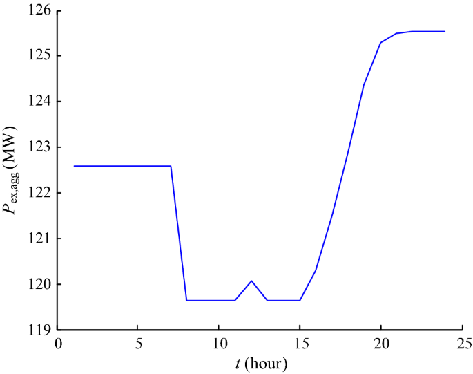
TCLs’ heat exchange power with the outside

The ideal \(E_{\text{agg}}^{\hbox{max} }\)of TCLs is 1.25×10⁵ kWh, calculated using (39). However, it is difficult for the indoor temperature Tin to reach the maximum or the minimum, so when considering the upper or lower limit of the energy storage, 5% of the ideal energy storage limit is set aside.
The scheduling results are shown in Figs. 5, 6, 7, from which we can draw the following conclusions:

Scheduling results of model I

Scheduling results of model II

Scheduling results of model III
-
1)
From Fig. 5, in the day-head scheduling model without considering the equivalent energy storage model, though the Pc,agg is constrained within limits, the maximum Eagg reaches 4×10⁵ kWh, far beyond the energy storage range. Further, the minimum is negative, which obviously disagrees with the facts. It indicates that in this situation, TCLs are not sufficient to meet the scheduling requirements, which will not be conducive to the reliable operation of the system.
-
2)
It is obviously seen that as the calculation methods of Pc,agg are different; in Figs. 5b and 6b, the limits of Pc,agg are always constant, while in Fig. 7b, the limits of Pc,agg change with time because of the time-varying characteristics.
-
3)
In Figs. 6 and 7, when the equivalent energy storage model is taken into account, though the loads participating in scheduling are decreased, the limits of the energy storage are constrained in a safe range because these two models both consider the actual ability of TCLs participating in scheduling. This shows that it is significant to introduce the equivalent energy storage model into the day-ahead scheduling model.
The results of the day-ahead scheduling will provide the basis for the actual control of TCLs. Within a day’s actual control, TCLs will carry out the load tracking control according to the power determined by the day-ahead scheduling, to make the aggregate power of TCLs as close to the result of the scheduling as possible [15].
In the following examples, the results of the load tracking control are compared, as shown in Figs. 8, 9, 10.

Load tracking control results of model I

Load tracking control results of model II

Load tracking control results of model III
The state of charge (SOC) of the equivalent energy storage model is represented by SOC, and SOC at time t is defined as follows.
where E′agg(t) is the aggregated energy storage obtained by the tracking control.
From Figs. 8, 9, 10, the following conclusions can be obtained.
-
1)
In Fig. 8, as the equivalent energy storage model is not considered, and the load tracking control cannot always accurately track Pc,agg obtained in Fig. 5b. During 7–10 h and 15–24 h, the load tracking control fails and SOC is either close to or even more than 1, or infinitely close to 0, which indicates again that the potential of TCLs has been exhausted, and it is not possible to participate fully in scheduling. Once again, the necessity of considering the equivalent energy storage model is explained.
-
2)
In Fig. 9, the equivalent energy storage model is considered, but Pc,agg is obtained by Pa,agg, which is a constant. Although the scheduling results of Fig. 6b can be tracked well most of the time, it fails during 19–21 h, and SOC is close to 0 at this moment. On the one hand, it is effective to introduce the equivalent energy storage model to some extent; on the other hand, it is not accurate enough to obtain Pc,agg directly by Pa,agg, and it is still detrimental to the stable operation of the power grid.
-
3)
Figure 10 adopts the proposed method. Not only is the scheduling result accurately tracked all the time, but SOC is also constrained within 0–1, which indicates that after adopting the time-varying Pex,agg and establishing its relationship with Eagg, the proposed model benefits the stable operation of the system.
In order to clearly show the accuracy of the load tracking control results, the integrated square error (ISE) is adopted, as shown in (43).
where P′c,agg is the power obtained by the tracking control; Pc,agg is the power obtained by the scheduling.
The results are shown in Table 2, from which we can see that ISE of model III (the proposed model) is the smallest, and is far smaller than the other two models. Again, this indicates that it is important to introduce the proposed equivalent energy storage model into the scheduling model.
Further, to compare the influence of the constraint percentage of the energy storage in the scheduling model on the load tracking control results, ISE is adopted to show the differences, as shown in Table 3.
From Table 3, when the constraint percentage is smaller than 5%, ISE tends to be larger because the scheduling results are not tracked well. Further, another reason is that the temperature cannot reach the maximum or the minimum, and so the energy storage cannot reach 100% or 0%. When the constraint percentage is higher than 5%, ISE tends to be smaller. However, in this case, the potential of TCLs is not fully realized because the energy storage is too constraining. Though the load tracking control performs well, TCLs participating in the scheduling will decrease significantly, resulting in a decrease in the advantage of TCLs participating in the scheduling.
5 Conclusion
In this paper, the large numbers of TCLs are modeled by the equivalent energy storage model and participate in day-ahead scheduling. The main contributions of this paper can be summarized as follows:
-
1)
The time-varying heat exchange power is adopted to calculate the charging and discharging power instead of the average power, to reflect the time-varying characteristics and improve the accuracy.
-
2)
The relationship between the heat exchange power and the aggregate energy storage is established in the equivalent energy storage model, compared to other energy storage models, which leads to a time-varying upper/lower limit of the charging and discharging power.
-
3)
The day-ahead scheduling model based on the equivalent energy storage model is proposed to effectively avoid the TCLs’ power and energy storage beyond the range. By load tracking control, the scheduling results can be tracked precisely. The testing results have shown the significance of the proposed model, and the model can improve the safety and reliability of the power grid.
Though the proposed scheduling model can provide comparatively accurate scheduling results, when characterizing the dynamics of TCLs, the second-order ETP model is more complex but more accurate than the first-order ETP model adopted in the proposed model. In the future work, we will try to establish a new energy storage model based on the second-order ETP model, and introduce it to the day-ahead scheduling model, in order to further improve the accuracy of scheduling.
References
Lowery C, O’Malley M (2012) Impact of wind forecast error statistics upon unit commitment. IEEE Trans Sustain Energy 3(4):760–768
Zhang Y, Wang J, Ding T et al (2018) Conditional value at risk-based stochastic unit commitment considering the uncertainty of wind power generation. IET Gener Transm Distrib 12(2):482–489
Wu J, Zhang B, Jiang Y (2018) Optimal day-ahead demand response contract for congestion management in the deregulated power market considering wind power. IET Gener Transm Distrib 12(4):917–926
Lu N, Zhang Y (2013) Design considerations of a centralized load controller using thermostatically controlled appliances for continuous regulation reserves. IEEE Trans Smart Grid 4(2):914–921
Shao S, Pipattanasomporn M, Rahman S (2011) Demand response as a load shaping tool in an intelligent grid with electric vehicles. IEEE Trans Smart Grid 2(4):624–631
Ashok S, Banerjee R (2003) Optimal operation of industrial cogeneration for load management. IEEE Trans Power Syst 18(2):931–937
Xu Z, Østergaard J, Togeby M (2011) Demand as frequency controlled reserve. IEEE Trans Power Syst 26(3):1062–1071
Chai B, Costa A, Ahipasaoglu SD et al (2018) Optimal meeting scheduling in smart commercial building for energy cost reduction. IEEE Trans Smart Grid 9(4):3060–3069
Luo F, Dong ZY, Meng K et al (2017) An operational planning framework for large-scale thermostatically controlled load dispatch. IEEE Trans Industrial Informatics 13(1):217–227
Luo F, Zhao JH, Dong ZY et al (2016) Optimal dispatch of air conditioner loads in Southern China region by direct load control. IEEE Trans Smart Grid 7(1):439–450
Jo H, Kim S, Joo S (2013) Smart heating and air conditioning scheduling method incorporating customer convenience for home energy management system. IEEE Trans Consum Electron 59(2):316–322
Song M, Gao C, Yan H et al (2017) Thermal battery modeling of inverter air conditioning for demand response. IEEE Trans Smart Grid. https://doi.org/10.1109/tsg.2017.2689820
Hao H, Sanandaji BM, Poolla K et al (2013) A generalized battery model of a collection of thermostatically controlled loads for providing ancillary service. In: Proceedings of 2013 51st annual Allerton conference on communication, control, and computing (Allerton), Monticello, USA, 2–4 October 2013, pp 551–558
Sanandaji BM, Hao H, Poolla K et al (2014) Improved battery models of an aggregation of thermostatically controlled loads for frequency regulation. In: Proceedings of 2014 American control conference, Portland, USA, 4–6 June 2014, pp 38–45
Hao H, Sanandaji BM, Poolla K et al (2015) Aggregate flexibility of thermostatically controlled loads. IEEE Trans Power Systems 30(1):189–198
Mathieu JL, Kamgarpour M, Lygeros J et al (2015) Arbitraging intraday wholesale energy market prices with aggregations of thermostatic loads. IEEE Trans Power Syst 30(2):763–772
Trovato V, Tindemans SH, Strbac G (2014) Security constrained economic dispatch with flexible thermostatically controlled loads. In: Proceedings of IEEE PES innovative smart grid technologies, Europe, Istanbul, Turkey, 12–15 October 2014, pp 1–6
Lu N (2012) An evaluation of the HVAC load potential for providing load balancing service. IEEE Trans Smart Grid 3(3):1263–1270
Perfumo C, Kofman E, Braslavsky JH (2012) Load management: model-based control of aggregate power for populations of thermostatically controlled loads. Energy Convers Manag 55(3):36–48
Wai CH, Beaudin M, Zareipour H (2015) Cooling devices in demand response: a comparison of control methods. IEEE Trans Smart Grid 6(1):249–260
Wu H, Guan X, Zhai Q (2009) Security-constrained generation scheduling with feasible energy delivery. In: Proceedings of 2009 IEEE PES general meeting, Calgary, Canada, 26–30 July 2009, pp 1–6
Wu HY, Shahidehpour M, Khodayar ME (2013) Hourly demand response in day-ahead scheduling considering generating unit ramping cost. IEEE Trans Power Syst 28(3):2446–2454
Callaway DS (2009) Tapping the energy storage potential in electric loads to deliver load following and regulation, with application to wind energy. Energy Convers Manag 50(5):1389–1400
Acknowledgement
This work was supported in part by the Postgraduate Innovation Cultivating Project in Jiangsu Province (No. KYCX18_1221), the National Natural Science Foundation of China (No. 51707099), China Postdoctoral Science Foundation (No. 2017M611859).
Author information
Authors and Affiliations
Corresponding author
Additional information
CrossCheck date: 6 September 2018
Rights and permissions
Open Access This article is distributed under the terms of the Creative Commons Attribution 4.0 International License (http://creativecommons.org/licenses/by/4.0/), which permits unrestricted use, distribution, and reproduction in any medium, provided you give appropriate credit to the original author(s) and the source, provide a link to the Creative Commons license, and indicate if changes were made.
About this article

Cite this article
CHEN, P., BAO, YQ., ZHU, X. et al. Day-ahead scheduling of large numbers of thermostatically controlled loads based on equivalent energy storage model. J. Mod. Power Syst. Clean Energy 7, 579–588 (2019). https://doi.org/10.1007/s40565-018-0468-3
Received:
Accepted:
Published:
Issue Date:
DOI: https://doi.org/10.1007/s40565-018-0468-3