
Abstract
Assembly plays an important role in any production system as it constitutes a significant portion of the lead time and cost of a product. Virtual computer-integrated manufacturing (VCIM) system is a modern production system being conceptually developed to extend the application of traditional computer-integrated manufacturing (CIM) system to global level. Assembly scheduling in VCIM systems is quite different from one in traditional production systems because of the difference in the working principles of the two systems. In this article, the assembly scheduling problem in VCIM systems is modeled and then an integrated approach based on genetic algorithm (GA) is proposed to search for a global optimised solution to the problem. Because of dynamic nature of the scheduling problem, a novel GA with unique chromosome representation and modified genetic operations is developed herein. Robustness of the proposed approach is verified by a numerical example.
Introduction
To succeed in the competitive market, nowadays, manufacturing enterprises need to be able to provide higher quality services with lower cost in shorter time. These requirements have forced a large number of manufacturing enterprises to apply advanced manufacturing technologies in various types to improve their performances (Gunawardana 2006). In general, the Advanced Manufacturing Technology (AMT) is defined as technology associated with computer software and hardware, and numerical based apparatus which are designed to accomplish or support manufacturing tasks (Costa et al. 2000).
There are a number of criteria to classify the AMTs, such as the level of integration, functional application, nature of apparatus, level of organisational integration, and imbedded information processing capabilities (Costa et al. 2000). Based on the degree of integration, AMTs are classified into three levels: stand-alone level, such as computer-aided design (CAD), computer numerical control (CNC) or computer-aided process planning (CAPP), intermediate level, such as manufacturing resource planning (MRP), automated inspection and testing systems (AITS) or automated material handling systems (AMHS), and integrated level, such as flexible manufacturing cell (FMC), flexible manufacturing system (FMS) or computer-integrated manufacturing (CIM) (Suresh and Meredith 1985; Small and Yasin 1997). As fully integrated system, CIM is of significant potential in modern manufacturing industry (Nagalingam and Lin 1999).
Computer-integrated manufacturing is a modern manufacturing system in which computers are used to control the production processes. All units of a CIM system are connected to each other by a computer network; therefore, the manufacturing system can be more efficient (Miller et al. 2010). Integration of AMTs makes CIM systems very effective (Nagalingam and Lin 1999). Nevertheless, CIM systems are capable of exploiting local resources only (Wang 2007). To overcome this limitation of CIM, a new system called virtual computer-integrated manufacturing (VCIM) is being developed. VCIM is a pretty new concept, defined as a network of interconnected CIM systems which are globally and/or locally distributed (Nagalingam and Lin 1999).
Assembly plays an important role in any production system as it involves the lead time and cost of a product. As a production system, VCIM always requires assembly operations. Traditionally, assembly planning and scheduling problems are often associated with finding assembly sequence and assembly resource location (Nof 1997). Assembly planning and scheduling in a VCIM system is quite different from ones in traditional production systems because the working principle of VCIM systems is different. In VCIM systems, it is required to find not only assembly sequence and assembly resource locations but also which assembly agent, manufacturing agent, and transportation plan to be used. Without connection with selections of manufacturing agent, assembly agent, and transportation plan, the assembly scheduling in a VCIM system is devoid of meaning. Literature review shows that there have been a large number of works on assembly planning and scheduling in traditional production systems. However, there have been no such works in VCIM systems yet. In this paper, assembly scheduling problem in VCIM systems is taken into consideration.
Literature review
With some unique characteristics inheriting from two major concepts: Virtual Enterprise and Computer-Integrated Manufacturing, virtual computer-integrated manufacturing (VCIM) is a promising solution for many small and medium size enterprises worldwide in the global market. The VCIM system is a modern concept in manufacturing industry proposed by Lin (Lin, G.C.I., the latest research trends in CIM, in the Fourth International Conference on Computer Integrated Manufacturing 1997) with the aim to overcome the limitation of traditional CIM system as it only works within a company. Major advantage of VCIM systems is the capability of effective sharing of distributed resources both locally and globally. This concept is still being developed and attracting a number of researchers.
In a VCIM system, there are three kinds of agents, namely resource agent, facilitator agent, and customer agent. The resource agent here could be manufacturing unit, assembly unit, material supplier, shipping provider, etc. VCIM systems work as follows. When a VCIM system receives a product order, the customer agent passes the product request to the facilitator agent. The facilitator agent then decomposes the product into a number of independent components. After that, the facilitator agent chooses some suitable resource agents for producing the decomposed components of the requested product and also chooses an assembly agent for assembling the product. In addition, the resource agent will ship the finished components as well as product to the required destinations to fulfil the product order (Zhou et al. 2010; Wang et al. 2003, 2004, 2004, 2007, 2005; Nagalingam et al. 2007).
The VCIM working principle indicates that an important issue to running a VCIM system is to organise the resources to fulfil customer orders; this issue is called resource scheduling. It can be clearly seen that this resource scheduling problem involves the task allocation, manufacturing sequence, assembly sequence, and supply chain management in a very dynamic environment. Resource scheduling is important to VCIM systems because it directly affects the lead time, cost, and quality of products. However, the research dealing with this scheduling problem is still limited. A number of works based on multi-agent approach (Zhou et al. 2007, 2010a, b, 2011; Wang et al. 2003, 2004, 2005) have been done to model VCIM systems. In addition, backward network algorithm (Wang et al. 2007; Nagalingam et al. 2007) has been proposed for the VCIM resource scheduling optimisation. Nevertheless, the optimal manufacturing sequence and assembly sequence have not been addressed in the scheduling model yet. In addition, the backward network algorithm cannot find a global optimised solution due to the way of forming a full schedule. Given that the sub-schedule for every single sub-task is optimised, no one can guarantee that the full resource schedule formed by adding optimal sub-schedules without modification is globally optimised.
Recently, an innovative resource scheduling model (Dao et al. 2016) was developed for VCIM system, in which the collaborative transportation scheduling is included in the traditional VCIM resource scheduling model; however, this model can handle only one product order at a time. A more advanced model (Dao et al. 2016), which is not only capable of supporting the collaborative transportation scheduling but also handling multiple product orders simultaneously, was also developed; nevertheless, this is a deterministic model and uncertainty is not taken into account yet. In addition, a stochastic model for resource scheduling in VCIM systems was proposed by (Dao et al. 2016), in which one product order is processed at a time. As can be seen, several aspects of the VCIM resource scheduling have been solved. However, no one has attempted to attack the assembly scheduling problem in VCIM systems. In the previous publications, the VCIM assembly scheduling problem was too simplified and/or overlooked.
Assembly scheduling is very important to any production system. There have been a significant number of research works about optimisation of the assembly scheduling for traditional production systems. This class of optimisation problems has been solved by various approaches, such as heuristic (Andrés et al. 2008; Kim et al. 1996; Al-Anzi and Allahverdi 2007; Allahverdi and Al-Anzi 2009; Sung and Kim 2008; Koulamas and Kyparisis 2001), particle swarm optimisation (Dong et al. 2012; Wang and Liu 2010; Hamta et al. 2013; Allahverdi and Al-Anzi 2006), mixed integer programming (Ozturk et al. 2010; Lin and Liao 2012; Terekhov et al. 2012; Sawik 2004), genetic algorithm(Wong et al. 2009; Marian et al. 2003, 2006; Yolmeh and Kianfar 2012; Celano et al. 1999; Dini et al. 1999), Taguchi method (Chen et al. 2010), dynamic programming (Jiang et al. 1997; Zhang et al. 2005; Yee and Ventura 1999), neural networks (Chen et al. 2008; Hong and Cho 1995), multi-agent evolutionary algorithm (Zeng et al. 2011), simulated annealing (Milner et al. 1994), etc. In general, all of the works done so far deal with two main optimisation issues: assembly sequence and assembly resource location. But optimisation of assembly scheduling in VCIM systems requires more issues than that. Besides the two issues mentioned above, VCIM systems require to find which assembly agent, manufacturing agent, and transportation plan to be used. It should be noted that these five issues must be solved simultaneously in VCIM systems. Otherwise, the schedule might not be feasible.
To solve large-scale complex optimisation problems, meta-heuristics are the popular choices (Abtahi and Bijari 2016; Javanmard and Koraeizadeh 2016; Moradgholi et al. 2016). There have been a large number of meta-heuristics, such as simulated annealing, tabu search, ant colony optimisation, particle swarm optimisation, genetic algorithm, swarm intelligence, artificial bee colony, cuckoo search, etc. Genetic algorithm (GA) is one of the most popular meta-heuristics (Paul et al. 2015). GA has several advantages, such as flexibility in defining constraints, capability of working with both continuous and discrete variables, capability of handling large search space, etc. (Fahimnia et al. 2008). However, GA is only a general search philosophy; there is no general GA capable of working best for every problem, and the problem-specific customisation in chromosome encoding and genetic operations is always required (Dao et al. 2014).
To overcome those limitations, this article focuses on the optimisation of assembly scheduling in VCIM systems using genetic algorithm (GA). Because of dynamic nature of the assembly scheduling problem in VCIM systems, a novel GA with unique chromosome representation and modified genetic operations is developed herein.
Problem statement
Based on the published works (Wang 2007; Zhou et al. 2010; Wang et al. 2007; Nagalingam et al. 2007; Wang et al. 2004; Wang et al. 2003a, b, 2004a, b; 2005; Zhou et al. 2007, 2010, 2011), assembly scheduling problem in VCIM systems is modeled herein as follows.
Consider:
-
A VCIM system is capable of producing P different types of products.
-
Each product can be decomposed into a number of parts or groups of parts, which are referred to as Parts in the rest of this paper.
-
There are A assembly agents and M manufacturing agents in the VCIM system, which are locally and/or globally distributed.
-
Each manufacturing agent can produce a limited number of different Parts for a certain number of different products.
-
Each assembly agent can assemble a limited number of different products.
-
There is a product order with delivery deadline and destination in the next period of time.
Determine:
Which manufacturing agents, which manufacturing sequences in the selected manufacturing agents, which assembly agent, and which assembly sequence in the selected assembly agent should be selected to create a temporary integrated production system in the VCIM system to fulfil the product order?
So that:
Cost of the requested product is minimised while all given constraints are satisfied.
Conditions:
-
Transportation cost and transportation time between any two locations are known in advance. These cost and time do not depend on the volume of the objects transported.
-
The product information such as the number of Parts to be decomposed, which manufacturing agents are capable of producing the decomposed Parts, which assembly agents are capable of assembling the product and precedence conditions for assembly operation is given in advance.
-
Manufacturing time and manufacturing cost of a Part produced by different manufacturing agents are not the same but given in advance.
-
Assembly cost and assembly time in different assembly agents are not the same but given in advance.
-
There are manufacturing changeovers in the manufacturing agents which take a given amount of time. Moreover, these changeovers are different in the different agents.
-
Assembly changeover will be applied if two adjacent assembly operations are relatively different. The changeover takes a certain amount of time and it is different in different assembly agents.
-
After a Part is made, it is directly transported to the selected assembly agent.
-
All agents in the VCIM system have enough resources to function and they are capable of working 24 h a day, 7 days a week.
The proposed assembly scheduling model for VCIM systems is illustrated in Fig. 1.

Proposed assembly scheduling model for VCIM systems
Proposed genetic algorithm
As mentioned before, genetic algorithm (GA) is only a general search philosophy; there is no general GA capable of working best for every problem, and the problem-specific customisation in chromosome encoding and genetic operations is always required (Dao et al. 2014). To solve the VCIM assembly scheduling problem, which is very complex because many precedence constraints are involved, a GA with many customisations must be developed. In this article, an innovative GA with a special chromosome encoding, two modified crossovers and two modified mutations is proposed to solve the problem. There are five main components of the proposed GA, i.e. chromosome encoding, crossover, mutation, evaluation, and selection. Details of the components will be explained in the next Sections.
Chromosome encoding
As the nature of the problem, a chromosome encoding a solution to the problem has three parts. The first part encodes the assembly agent selection. An example of the first part for the VCIM system with seven assembly agents is shown in Table 1. This example is associated with product 3 and assembly agent 4 is selected. The second part represents the assemble sequence in the selected assembly agent as shown in Table 2. In this example, product 3 has been decomposed into 25 Parts denoted by integer numbers from 1 to 25. It is noted that detailed information about the assemble operations cannot be expressed in Table 2. Therefore, supplemental information is needed as shown in Table 3. The positive integer numbers in Table 3 represent the sequence of assembly operations. For example, number “1” shows that the Part 1 and Part 4 are assembled together first and number “2” indicates that Part 6 is assembled to Part 1 next, and so on. The last part of a chromosome is for manufacturing agent selection expressed by binary number as shown in Table 4. It is noted that some manufacturing agents, for example agent 2, are selected for a number of times to produce several Parts. In those cases, manufacturing sequence is expressed by the top-down order. For example, the manufacturing sequence in agent 2 in Table 4 is as follows: Part 2, Part 4, Part 18 and then Part 19.
In addition, at this stage, it is assumed that every Part is transported to the selected assembly agent right after it is made and there is no transport option. Therefore, transportation plan comes strictly after the agents selected.
Automatic generation of such chromosome is not easy due to a lot of complex constraints involved. This scheduling problem involves a lot of hard precedence constraints that makes the solution infeasible if violated. According to Marian (Marian 2003), this kind of constraint is generally divided into two categories: internal precedence constraint and external precedence constraint. The internal is precedence constraint derived from configuration of the product while the external precedence constraint originates from assembly process such as assembly line layout or supply of parts. In this paper, the internal precedence constraints are expressed in Assembly Table as shown in Table 5, for example. In Table 5, “0” means no connection between pi and pj; “1” means pi and pj can be assembled at any stage; “xk” is a reference liaison; and “>xk” represents that the corresponding assembly operation has to be done after the reference liaison “xk” has been established. For example, Part 18 can only be assembled to Part 1 if Part 10 has already been assembled to Part 1. To generate a feasible chromosome, the following steps are proposed:
Step 1: Randomly select one assembly agent among the suitable ones
Step 2: Randomly select a Part among the decomposed Parts of the product
Step 3: Remove the corresponding column of the selected Part in Step 2 from the Assembly Table.
Step 4: Randomly select a manufacturing agent among the suitable ones to produce the selected Part in Step 2.
Step 5: Determine the Part candidates for the next assembly operation based on the assembly rule in the updated Assembly Table.
Step 6: Randomly select one Part among the suitable ones in Step 5.
Step 7: Remove the corresponding column of the selected Part in Step 6 from the updated Assembly Table.
Step 8: Randomly select one manufacturing agent among the suitable ones to produce the selected Part in Step 6.
Step 9: Repeat Steps 5–8 until all Parts of the product have been selected.
Step 10: Check the product completion time against the deadline. If it meets the requirement, one feasible chromosome has been generated. Otherwise, repeat Steps 1–10 until a feasible one is achieved.
It should be noted that the sizes of parts 2 and 3 of a chromosome are variable as different products might be decomposed into a different number of Parts.
Crossover
In principle, crossover is a simple cut and swap operation (Gen and Cheng 1997). However, because of the hard precedence constraint and nature of the chromosome as shown in Sect. 4.1, a modified crossover operation is required. To handle the complex constraints and to enhance the search efficiency, the proposed GA with two crossover operations, namely crossover 1 and crossover 2, is proposed herein. Details of the two crossover operations will be explained in the next Sections.
Crossover 1
The crossover 1 is applied to part 1 of a chromosome. To implement the crossover operation, the following steps are proposed:
Step 1: Randomly select two parent chromosomes.
Step 2: Determine the first parts of the selected chromosomes in Step 1.
Step 3: Randomly select one cut point, somewhere between the first column and the smallest column containing value 1 (column 3 in Table 6, for example); otherwise the crossover operation has no effect or leads to infeasible offspring chromosomes.
Step 4: Swap the two pieces as illustrated in Table 6.
Step 5: Form the complete offspring chromosomes accordingly.
Step 6: Check the completion time constraints. If at least one constraint is not satisfied, go back to Step 1; otherwise, stop.
Crossover 2
The crossover 2 is applied to part 2 of a chromosome. As many hard constraints involved, the following steps are proposed to implement the crossover 2.
Step 1: Randomly select two parent chromosomes.
Step 2: Determine the second parts of the selected chromosomes in Step 1.
Step 3: Randomly select one cut point as illustrated in Table 7.
Step 4: Swap the two pieces as shown in Tables 7 and 8.
Step 5: Repair the second parts of the offspring chromosomes. Unlike the crossover 1, it is required to repair the children chromosomes after the crossover 2 applied as they are usually infeasible because of hard precedence constraints involved and other issues. For example, after crossover 2 applied, there are two Parts number 3, 10, 14 or 21 in the part 2 of the offspring chromosome as shown in the first sub-table in Table 7. The repair principle used in this paper has been proposed by Marian et al. (2000, 2006; Marian 2003) as follows: Every gene after the cut point must be checked against the feasibility based on recorded information about all of the previous assembly operations, not just the adjacent one. If feasible, a gene is accepted; otherwise a new one is randomly generated based on the precedence constraints in the Assembly Table and the previous assembly operations, and then a new suitable manufacturing agent is randomly selected to produce the Part in this new gene (the third parts of the offspring chromosomes will be updated accordingly). After repair operation applied, the offspring chromosomes are feasible and look like as shown in Table 8. It is noted that differences between the infeasible and feasible offspring can be seen when comparing Table 7 with Table 8.
Step 6: Form the complete offspring chromosomes accordingly.
Step 7: Check the completion time constraints. If at least one constraint is not satisfied, go back to Step 1; otherwise, stop.
It should be noted that although crossover 2 is applied to part 2 of the parent chromosomes, it also has some effect on the corresponding part 3 as indicated in Step 5.
Mutation
In general, mutation is an operation of altering one or more genes (Gen and Cheng 1997). Again, as the hard precedence constraint and nature of the chromosome as shown in Sect. 4.1, a modified mutation operation is required. Similar to crossover, mutation only applied to the first two parts of a chromosome is proposed herein.
Mutation 1
Mutation 1 is applied to part 1 of a chromosome. It should be noted that unlike the crossover 1, the mutation 1 is performed on one parent chromosome only. Due to constraints involved, the following steps are proposed to implement mutation 1.
Step 1: Randomly select one parent chromosome.
Step 2: Determine the first part of the selected chromosome in Step 1.
Step 3: Determine the first gene with value of 1.
Step 4: Randomly select the second gene with value of 0.
Step 5: Exchange the two genes in Steps 3–4 as illustrated in Table 9.
Step 6: Check the feasibility of the first part of the offspring chromosome. If feasible, go to Step 7, otherwise, go back to Step 4.
Step 7: Form the complete offspring chromosome accordingly.
Step 8: Check the completion time constraint. If the constraint is not satisfied, go back to Step 1; otherwise, stop.
Mutation 2
Mutation 2 of the proposed GA is applied to the second parts of chromosomes. Similar to crossover 2, the offspring chromosomes of mutation 2 need to be repaired to make them feasible. To implement the mutation 2, the following steps are proposed:
Step 1: Randomly select two parent chromosomes.
Step 2: Determine the second parts of the selected chromosomes in Step 1.
Step 3: Randomly select two genes, the highlighted ones in Table 10, for example.
Step 4: Exchange the two selected genes as illustrated in Table 11.
Step 5: Repair the second parts of the offspring chromosomes. All of the genes from the selected genes for Mutation 2 to the end must be checked against the feasibility, the so called feasible-gene checking, and repaired if necessary. For examples, the genes from column 17–25 and from column 5–25 as shown in the first and second sub-tables, respectively, in Table 11 must be checked and repaired if necessary. It is noted that the feasible-gene checking is based on recorded information about all of the previous assembly operations, not just the adjacent ones. The repair principle used here is exactly the same as presented in Sect. 4.2.2. That is, a gene is accepted if feasible; otherwise a new one is randomly generated based on the precedence constraints in the Assembly Table and previous assembly operations (Marian et al. 2006; Marian 2003; Marian, R., L. Luong, and K. Abhary, A new crossover technique for assembly sequence planning using GA, in The 5th International Conference on Computer Integrated Manufacturing 2000), and then a new suitable manufacturing agent is randomly selected to produce the Part in this new gene (the third parts of the offspring chromosomes will be updated accordingly). After repaired, the offspring chromosomes are feasible and look like as shown in Table 12. The differences between infeasible and feasible offspring are highlighted in red colour in Table 12.
Step 6: Form the complete offspring chromosomes accordingly.
Step 7: Check the completion time constraints. If at least one constraint is not satisfied, go back to Step 1; otherwise, stop.
It should be noted that although mutation 2 is applied to part 2 of the parent chromosomes, it also has some effect on the corresponding part 3 as indicated in Step 5.
Evaluation
Quality of the solution to the problem is evaluated through objective function—cost of the product. Obviously, the smaller the cost is, the better it is. The cost of a product is calculated as follows
where: C is the cost of a product; MC is the total manufacturing cost; TC1 is the total transportation cost for transporting all of the Parts of a product from the manufacturing agents to the assembly agent; AC is the total assembly cost; TC2 is transportation cost for transporting the finished product to customer.
Selection
In the proposed GA, a new population is selected for next generation by Roulette Wheel approach. This approach selects a new population based on the probability distribution associated with fitness values of chromosomes (Gen and Cheng 1997). In addition, the power law scaling for objective function proposed by Gillies (Gillies 1985) is also used with Roulette Wheel approach to improve the performance of the GA.
The proposed GA has the classical structure. Robustness of the GA is demonstrated by a comprehensive case study.
Numerical example
Problem description
Consider:
-
A VCIM system is capable of producing ten different products.
-
Each product can be made by assembling a number of Parts as shown in Table 13.
Table 13 Quantity of decomposed Parts -
There are seven assembly agents and 13 manufacturing agents in the VCIM system.
-
There is a customer requesting product 3 and requiring its delivery deadline to be within 5 days, for example. Without losing generality, it is assumed that the product 3 is a body of the modified hydraulic linear motor designed by Marian (Marian, R., Research and contributions concerning the improvement of a hydraulic linear motor with piston valves, in Technical Report 1996). This product was chosen for its model availability, size and complexity. The product 3 has 25 components as shown in Fig. 2.
Fig. 2 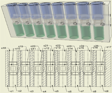
Body of the modified hydraulic linear motor [64]
-
Capabilities of manufacturing agents are shown in Tables 14 and 15. The symbol “–” in Tables 14 and 15 means that the corresponding agent is not capable of producing the corresponding Part. It is noted that only a part of Tables 14 and 15 is presented herein due to the lengthiness.
Table 14 Manufacturing cost ($) Table 15 Manufacturing time (hour) -
Capabilities of assembly agents are shown in Table 16. The symbol “–” in Table 16 means that the corresponding agent is not suitable for the corresponding product.
Table 16 Functionalities of assembly agents -
Transportation cost and transportation time between a manufacturing agent and an assembly agent are given in Tables 17 and 18.
Table 17 Transportation cost between manufacturing agent and assembly agent ($) Table 18 Transportation time between manufacturing agent and assembly agent (hour) -
Transportation cost and transportation time between assembly agent and the customer are shown in Tables 19 and 20.
Table 19 Transportation cost between assembly agent and the customer ($) Table 20 Transportation time between assembly agent and the customer (hour) -
Precedence condition of product 3 for its assembly implementation is given in Table 5.
-
Cost and time for different assembly operations for product 3 are assumed to be the same in any suitable assembly agent and shown in Tables 21 and 22.
Table 21 Assembly operation cost ($) Table 22 Assembly operation time (hour)

Determine:
Which manufacturing agents, which manufacturing sequences in the selected manufacturing agents, which assembly agent, and which assembly sequence in the selected assembly agent should be selected to create a temporary integrated production system in the VCIM system to fulfil the product order?
So that:
Cost of the product is minimised while all given constraints are satisfied.
Conditions:
-
The transportation cost and transportation time do not depend on the volume of the objects transported.
-
There are manufacturing changeovers in the manufacturing agents which take a given amount of time as shown in Table 23.
Table 23 Manufacturing changeover time (hour) -
Assembly changeover will be applied if two adjacent assembly operations are relatively different. The changeover takes a certain amount of time and it is different in different assembly agents as shown in Table 24. It is noted that in this case study there are three groups of assembly operations expressed by different values in Table 21. For example, the group 1 and 2 are with the assembly cost of 50 and 70, respectively.
Table 24 Assembly changeover time (hour) -
After a Part is made, it is directly transported to the selected assembly agent.
-
All agents in the VCIM system have enough resources to function and they are capable of working 24 h a day, 7 days a week.
Results and discussions
The proposed GA was implemented in Matlab software. Based on some test results, the parameters of the proposed GA were chosen as shown in Table 25 and the power scaling coefficient of objective function for the selection operator is 2. It is noted that the crossover and mutation rates in Table 25 are in terms of the number of chromosomes undergoing the crossover and mutation, respectively. Computing time of the proposed GA is less than 2 min for 400 generations. A typical evolution of fitness value is shown in Fig. 3. The best solution for the assembly scheduling problem with fitness value of 5855.0 achieved by the proposed GA is shown in Tables 26, 27, 28 and 29.

Typical evolution of fitness value by the proposed GA
Clearly, optimisation of assembly scheduling in VCIM systems is a multi-dimensional optimisation problem. It is required to optimise four dimensions at the same time: assembly agent selection, manufacturing agent selection, assembly sequence, and manufacturing sequence. There are four sub-problems to be optimised. If each sub-problem is solved at a time, the global optimised solution cannot be achieved. Therefore, an integrated scheduling approach as presented in this paper is required to obtain a global optimised solution.
As a heuristic search method, GA might not find the best solution after one run. That is because it can be caught in a local optimum, especially in multi-dimensional optimisation problems like the optimal assembly scheduling in VCIM systems. One of the most popular and easiest ways to overcome that problem is a procedure named Multistart, which is widely used in global optimisation. This procedure is simply to start the research algorithm with different starting points distributed over the whole optimisation region for a number of times. With GA, the first generation is totally generated at random. Therefore, GA just needs to be run for a number of times. In this case study, the Multistart was applied to the proposed GA and the solution shown in Tables 26, 27, 28 and 29 can be considered as a global optimised solution.
The case study shows that convergence of the proposed GA is quite sensitive to its parameters: crossover and mutation rate. That is because a lot of hard precedence constraints are involved. As mentioned before, this kind of constraint, if violated, will make the solution infeasible. After the crossover and mutation operations applied, the offspring chromosomes must be repaired to satisfy such hard precedence constraints. As a result, children chromosomes might not inherit much genetic information from their parents. In other words, offspring chromosomes are quite different from their parents. This causes the poor convergence of not just the proposed GA but all of other GAs dealing with a significant number of hard precedence constraints. A solution for this poor convergence problem proposed herein is to reduce crossover and mutation rates, increase population size, and use power scaling coefficient of objective function in selection operator. This approach can balance the exploitation and exploration abilities of the GA. However, selecting a set of appropriate values of those parameters is generally problem dependent.
To evaluate the effectiveness of the proposed GA, further experiments were carried out, in which performances of the proposed GA and random search method (Andradóttir, S., A review of random search methods, in Handbook of Simulation Optimization, C.M. Fu, Editor 2015) are compared to one another. Each method was independently run for ten times and the experimental results are shown in Table 30. It should be noted that stopping criteria of both the proposed GA and the random search method are in terms of the number of objective function evaluations; and they were set exactly the same as shown in Table 30. With that stopping criterion, the computing time of each run is about 2 min.
As can be seen from Table 30, on average, the proposed GA found the solutions with the total cost of $5987.0, while the average total cost of the solutions obtained by the random search method is $6398.0. In other words, the proposed GA can provide, on average, 6.4% better solution, compared to the random search method.
Conclusions
In this paper, a new class of assembly scheduling problems in VCIM systems has been modeled as an integrated scheduling problem. This schedule is associated with selections of assembly agent, manufacturing agent, assembly sequence, and manufacturing sequence. This problem belongs to multi-dimensional optimisation problem in which a number of sub-problems are required to be optimised at the same time. An integrated approach based on GA is proposed to search for a global optimised solution for the assembly scheduling problem. Because of the unique nature of the scheduling problem and constraints, a novel GA with unique chromosome representation, modified genetic operations has been developed herein.
Robustness of the proposed approach has been verified by an industrial-size case study. It took only about 2 min to obtain a good solution for such complicated scheduling problem in which a large number of complex constraints involved. On average, the proposed GA can provide 6.4% better solution, compared to the random search method. This proposed approach has a great potential in VCIM implementation.
In the future work, more case studies will be carried out to further verify the effectiveness of the proposed approach.
References
Abtahi AR, Bijari A (2016) A novel hybrid meta-heuristic technique applied to the well-known benchmark optimization problems. J Indust Eng Int 1–13. doi:10.1007/s40092-016-0170-x
Al-Anzi FS, Allahverdi A (2007) A self-adaptive differential evolution heuristic for two-stage assembly scheduling problem to minimize maximum lateness with setup times. Eur J Oper Res 182(1):80–94
Allahverdi A, Al-Anzi FS (2006) A PSO and a Tabu search heuristics for the assembly scheduling problem of the two-stage distributed database application. Comput Oper Res 33(4):1056–1080
Allahverdi A, Al-Anzi FS (2009) The two-stage assembly scheduling problem to minimize total completion time with setup times. Comput Oper Res 36(10):2740–2747
Andradóttir S (2015) A review of random search methods, in Handbook of Simulation Optimization. In: Fu CM (ed) Springer, New York pp 277–292
Andrés C, Miralles C, Pastor R (2008) Balancing and scheduling tasks in assembly lines with sequence-dependent setup times. Eur J Oper Res 187(3):1212–1223
Celano G et al (1999) An evolutionary approach to multi-objective scheduling of mixed model assembly lines. Comput Ind Eng 37(1–2):69–73
Chen W-C et al (2008) A three-stage integrated approach for assembly sequence planning using neural networks. Expert Syst Appl 34(3):1777–1786
Chen W-C et al (2010) A systematic optimization approach for assembly sequence planning using Taguchi method, DOE, and BPNN. Expert Syst Appl 37(1):716–726
Costa SGD, Platts K, Fleury A (2000) Advanced manufacturing technology: Defining the object and positioning it as an element of manufacturing strategy. In: VI International Conference on Industrial Engineering and Operations Management São Paulo, Brazil pp 1–8
Dao SD, Abhary K, Marian R (2014) Optimisation of partner selection and collaborative transportation scheduling in Virtual Enterprises using GA. Expert Syst Appl 41(15):6701–6717
Dao SD, Abhary K, Marian R (2016a) An innovative model for resource scheduling in VCIM systems. Operat Res Int J. doi:10.1007/s12351-016-0252-y
Dao SD, Abhary K, Marian R (2016b) An integrated production scheduling model for multi-product orders in VCIM systems. Int J Syst Assur Eng Manage. doi:10.1007/s13198-016-0504-5
Dao SD, Abhary K, Marian R (2016c) A stochastic production scheduling model for VCIM systems. Intell Indust Syst 2(1):85–101
Dini G et al (1999) Generation of optimized assembly sequences using genetic algorithms. CIRP Ann Manufact Technol 48(1):17–20
Dong Q, Lu J, Gui Y (2012) Integrated optimization of production planning and scheduling in mixed model assembly line. Procedia Eng 29:3340–3347
Fahimnia B, Luong L, Marian R (2008) Optimization/simulation modeling of the integrated production-distribution plan: an innovative survey. WSEAS Trans Business Econ 3(5):52–65
Gen M, Cheng R (1997) Genetic algorithms and engineering design. Wiley, New York
Gillies AM (1985) Machine learning procedures for generating image domain feature detectors. University of Michigan, Ann Arbor
Gunawardana KD (2006) Introduction of advanced manufacturing technology: a literature review. Sabaragamuwa Univ J 6(1):116–134
Hamta N et al (2013) A hybrid PSO algorithm for a multi-objective assembly line balancing problem with flexible operation times, sequence-dependent setup times and learning effect. Int J Prod Econ 141(1):99–111
Hong DS, Cho HS (1995) A neural-network-based computational scheme for generating optimized robotic assembly sequences. Eng Appl Artif Intell 8(2):129–145
Javanmard H, Koraeizadeh AAW (2016) Optimizing the preventive maintenance scheduling by genetic algorithm based on cost and reliability in National Iranian Drilling Company. J Indust Eng Int pp 1–8. doi:10.1007/s40092-016-0155-9
Jiang K, Seneviratne LD, Earles SWE (1997) Assembly scheduling for an integrated two-robot workcell. Robot Comp-Integr Manufact 13(2):131–143
Kim Y-D, Lim H-G, Park M-W (1996) Search heuristics for a flowshop scheduling problem in a printed circuit board assembly process. Eur J Oper Res 91(1):124–143
Koulamas C, Kyparisis GJ (2001) The three-stage assembly flowshop scheduling problem. Comput Oper Res 28(7):689–704
Lin GCI (1997) The latest research trends in CIM. In: The fourth international conference on computer integrated manufacturing. Singapore. pp 26–33
Lin R, Liao C-J (2012) A case study of batch scheduling for an assembly shop. Int J Prod Econ 139(2):473–483
Marian R (2003) Optimisation of assembly sequences using genetic algorithms. University of South Australia, Adelaide
Marian R, Luong L, Abhary K (2000) A new crossover technique for assembly sequence planning using GA. In: The 5th International Conference on Computer Integrated Manufacturing. Singapore. pp 723–733
Marian R (1996) Research and contributions concerning the improvement of a hydraulic linear motor with piston-valves. In: Technical Report, Technical University Cluj-Napoca, Cluj-Napoca, Romania
Marian R, Luong L, Abhary K (2003) Assembly sequence planning and optimisation using genetic algorithms: part I: automatic generation of feasible assembly sequences. Appl Soft Comput 2(3):223–253
Marian R, Luong L, Abhary K (2006a) A genetic algorithm for the optimisation of assembly sequences. Comput Ind Eng 50(4):503–527
Marian R, Luong L, Abhary K (2006b) A genetic algorithm for the optimisation of assembly sequences. Comput Ind Eng 50(4):503–527
Miller FP, Vandome AF, McBrewster J (2010) Computer-integrated manufacturing. VDM Publishing House, Mauritius
Milner JM, Graves SC, Whitney DE (1994) Using simulated annealing to select least-cost assembly sequences, in IEEE International Conference on Robotics and Automation. San Diego vol 3, pp 2058–2063
Moradgholi M et al (2016) A genetic algorithm for a bi-objective mathematical model for dynamic virtual cell formation problem. J Industr Eng Inte 12(3):343–359. doi:10.1007/s40092-016-0151-0
Nagalingam SV, Lin GCI (1999) Latest developments in CIM. Robot Comput-Integr Manufact 15(6):423–430
Nagalingam SV, Lin GCI, Wang D (2007) Resource scheduling for a virtual CIM system. In: Wang L, Shen W (eds) Process planning and scheduling for distributed manufacturing. Springer ,London pp 269–294
Nof SY, Wilhelm WE, Warnecke HH-J (1997) Industrial assembly. Chapman & Hall, London
Ozturk C et al (2010) Simultaneous balancing and scheduling of flexible mixed model assembly lines with sequence-dependent setup times. Electronic Notes in Discrete Mathematics 36:65–72
Paul PV et al (2015) Performance analyses over population seeding techniques of the permutation-coded genetic algorithm: an empirical study based on traveling salesman problems. Appl Soft Comput 32:383–402
Sawik T (2004) Loading and scheduling of a flexible assembly system by mixed integer programming. Eur J Oper Res 154(1):1–19
Small MH, Yasin MM (1997) Advanced manufacturing technology: implementation policy and performance. J Oper Manage 15(4):349–370
Sung CS, Kim HA (2008) A two-stage multiple-machine assembly scheduling problem for minimizing sum of completion times. Int J Prod Econ 113(2):1038–1048
Suresh NC, Meredith JR (1985) Justifying multimachine systems: an integrated strategic approach. J Manuf Syst 4(2):117–134
Terekhov D et al (2012) Solving two-machine assembly scheduling problems with inventory constraints. Comput Ind Eng 63(1):120–134
Wang D (2007) The development of an agent-based architecture for virtual CIM. University of South Australia, Adelaide
Wang D, Nagalingam SV, Lin GCI (2004) A parallel processing multi-agent architecture for virtual CIM system. In: Proceedings of the 14th International Conference on Flexible Automation and Intelligent Manufacturing. Toronto, Canada pp 1–9
Wang D, Nagalingam SV, Lin GCI (2003) Development of a virtual CIM system using agent-based approach, in Proceedings of the 7th International Conference on Mechatronics Technology. Taipei, Taiwan pp 445–450
Wang D, Nagalingam SV, Lin GCI (2003) Implementation approaches for a multi-agent virtual CIM system, in Proceedings of the 9th International Conference on Manufacturing Excellence. Melbourne, Australia pp 1–9
Wang D, Nagalingam SV, Lin GCI (2004) Production and logistic planning towards agent-based virtual CIM system in an SME network, in Eighth International Conference on Manufacturing and Management. Queensland, Australia pp 1–8
Wang Y, Liu JH (2010) Chaotic particle swarm optimization for assembly sequence planning. Robot Comp-Integr Manufact 26(2):212–222
Wang D, Nagalingam SV, Lin GCI (2004c) Development of a parallel processing multi-agent architecture for a virtual CIM system. Int J Prod Res 42(17):3765–3785
Wang D, Nagalingam SV, Lin GCI (2005) A novel multi-agent architecture for a virtual CIM system. Int J Agile Manuf 8(1):69–81
Wang D, Nagalingam SV, Lin GCI (2007) Development of an agent-based virtual CIM architecture for small to medium manufacturers. Robot Comput-Integ Manuf 23(1):1–16
Wong TC, Chan FTS, Chan LY (2009) A resource-constrained assembly job shop scheduling problem with Lot Streaming technique. Comput Ind Eng 57(3):983–995
Yee S-T, Ventura JA (1999) A Petri net model to determine optimal assembly sequences with assembly operation constraints. J Manufact Syst 18(3):203–213
Yolmeh A, Kianfar F (2012) An efficient hybrid genetic algorithm to solve assembly line balancing problem with sequence-dependent setup times. Comput Ind Eng 62(4):936–945
Zeng C et al (2011) A multi-agent evolutionary algorIthm for connector-based assembly sequence planning. Procedia Eng 15:3689–3693
Zhang W, Freiheit T, Yang H (2005) Dynamic scheduling in flexible assembly system based on timed Petri nets model. Robot Comp-Integr Manufact 21(6):550–558
Zhou N, Nagalingam SV, Lin GCI (2007) Application of virtual CIM in small and medium manufacturing enterprises. In: Hinduja S, Fan KC (eds) The 35th International MATADOR Conference. Springer, London. pp 161–164
Zhou N et al (2010) Development of an agent based VCIM resource scheduling process for small and medium enterprises. In: Proceedings of the international multiconference of engineers and computer scientists. Hong kong pp 39–44
Zhou N et al (2011) Inside virtual CIM: Multi-agent based resource integration for small to medium sized manufacturing enterprises. In: Ao SI, Castillo O, Huang X (eds) Intelligent Control and Computer Engineering. Springer, Netherlands pp 163–175
Zhou N, Xing K, Nagalingam SV (2010) An agent-based cross-enterprise resource planning for small and medium enterprises. IAENG Int J Comp Sci 37(3):1–7
Acknowledgement
The first author is grateful to Australian Government for sponsoring his PhD study at the University of South Australia, Australia in form of Endeavour Award.
Author information
Authors and Affiliations
Corresponding author
Rights and permissions
Open Access This article is distributed under the terms of the Creative Commons Attribution 4.0 International License (http://creativecommons.org/licenses/by/4.0/), which permits unrestricted use, distribution, and reproduction in any medium, provided you give appropriate credit to the original author(s) and the source, provide a link to the Creative Commons license, and indicate if changes were made.
About this article

Cite this article
Dao, S.D., Abhary, K. & Marian, R. Optimisation of assembly scheduling in VCIM systems using genetic algorithm. J Ind Eng Int 13, 275–296 (2017). https://doi.org/10.1007/s40092-017-0183-0
Received:
Accepted:
Published:
Issue Date:
DOI: https://doi.org/10.1007/s40092-017-0183-0