
Abstract
Event-related potential data can be used to index perceptual and cognitive operations. However, they are typically high-dimensional and noisy. This study examines the original raw data and six feature-extraction methods as a pre-processing step before classification. Four traditionally used feature-extraction methods were considered: principal component analysis, independent component analysis, auto-regression, and wavelets. We add to these a less well-known method called interval feature extraction. It overproduces features from the ERP signal and then eliminates irrelevant and redundant features by the fast correlation-based filter. To make the comparisons fair, the other feature-extraction methods were also run with the filter. An experiment on two EEG datasets (four classification scenarios) was carried out to examine the classification accuracy of four classifiers on the extracted features: support vector machines with linear and perceptron kernel, the nearest neighbour classifier and the random forest ensemble method. The interval features led to the best classification accuracy in most of the configurations, specifically when used with the Random Forest classifier ensemble.
1 Introduction
Event-related potentials (ERP) are stereotyped electrophysiological responses to a volitional activity or an external stimulus. ERPs are derived by averaging the spontaneous electroencephalogram (EEG) across several occurrences of the same event, for example, repeated presentations of the same stimulus. Assuming that the onset of the event is known, the ERP is a time series containing the ensuing brain reaction, termed an epoch. ERP can be used to distinguish between the brain states of the subject in response to the different stimuli within the particular examination context. This makes ERP analysis an ideal, long-standing tool in brain–computer interface (BCI) [2], ranging from predicting the laterality of imminent left- versus right-hand finger movements [1] to distinguishing between musical segments [22].
Classification of ERP data is challenging due to the high dimensionality and noise contamination of the raw data. Here, we study the classification accuracy of the original data and four feature-extraction methods used as a preprocessing step, and argue that ERP data benefits from interval feature extraction.
ERP are associated to different electrodes. For each electrode, a different classification problem is considered. The ERP time series is regarded as a collection of measurements, \(x_1,\ldots , x_T,\) each measurement is considered to be a feature. Thus, each ERP series becomes a point in a \(T\)-dimensional space, \(\mathbf x \in \mathfrak R ^T.\) A training dataset is a collection of points \(\mathbf x _1,\ldots \mathbf x _N\) and the corresponding labels \(y_1\dots y_N.\)
Section 2 explains the feature-extraction methods, Sect. 3 lists the four classifiers, and Sect. 4 details the data, the experimental protocol and the results.
2 Feature-extraction methods
2.1 The original (raw) data
A classification method is applied directly to the given training dataset: \(N\) data points \(\mathbf x _1,\ldots \mathbf x _N\) with \(\mathbf x _i\in \mathfrak R ^T\) and labels \(y_1\dots y_N.\)
To illustrate the difficulty in classifying ERP data, Fig. 1 shows 44 individual ERPs coming from an experiment where 22 participants viewed two categories of objects (classes or conditions): faces and cars. The grand-average ERPs for the two classes are plotted with thick lines. There is no clear pattern to guide the classifications.

Individual and grand-average ERP curves at electrode location POZ. The onset of the event is marked with a dashed line
2.2 PCA
Principal component analysis (PCA), independent component analysis (ICA) and auto-regression models (AR) are widely used feature-extraction methods in EEG/ERP data analysis [4, 7, 15, 16, 25].
PCA calculates a transformation matrix \(W\) such that the original features are replaced with extracted features, obtained as \(\mathbf a = W\mathbf x \). This effectively rotates the space so that the fist component of \(\mathbf a \) is orientated along the dimension with the largest variance in the data, the second component is orthogonal to the first one, and is orientated along the largest remaining variance, and so on. The number of retained components is determined so that a chosen percentage of the variance of the data is preserved after the transformation (we used 95 % in the experiments).
2.3 ICA
Independent component analysis also looks for a linear transformation of the original space in the form \(\mathbf a = W\mathbf x \) but the derivation of \(W\) is governed by a different criterion: the components of \(\mathbf a \) should be as independent as possible. Traditionally, ICA has been applied for the task of “blind source separation”, where a signal is decomposed into a weighted sum of independent source signals [4, 10], but there is no reason why we should stop here. Any feature set can be processed so as to derive a new smaller set of independent features. We used the FastICA algorithm due to Hyvärinen [9].Footnote 1
2.4 Auto-regression (AR)
Auto-regressive (AR) models regard the ERP as a dynamic system of order \(K\) where the \(i\)th value of the signal is predicted by the previous \(K\) values \(\hat{x}_i = a_1\,x_{i-K+1}+a_2\,x_{i-K+2}+\cdots +a_K\,x_{i-1}.\) The coefficients \(a_j\) are fitted to minimise the discrepancy between the prediction \(\hat{x}_i\) and the true value \(x_i,\) and treated as the extracted features. Models of order up to \(K=50\) have been considered [16].Footnote 2
2.5 Wavelets
A family of wavelets are scaled and shifted, so that the ERP signal is approximated in the best possible way. Wavelets capture both finer and coarser resolution features of the signal. The features which represent the ERP signal are the coefficients of the wavelets. Wavelet feature extraction has been widely applied to EEG analysis, opening up the perspectives of obtaining highly informative spatial-spectral-temporal descriptions [12]. The wavelet method has found its use in ERP analysis and classification also [14, 17, 18, 21, 28].
2.6 Interval features
Features derived from the signal over time segments of various lengths, called “interval features”, have been shown to lead to high classification accuracy [19, 20].
Denote by \(x_i\) the value of the signal at time \(i\), where \(i=1,\ldots ,T\) spans the ERP epoch. Nested time intervals are formed for each \(i\) using the remaining series \(x_i,\ldots ,x_T\). The interval length is varied as the power of two, while the starting point is kept at \(i\). Thus, the first interval at \(i\) is the point set \(\{x_i,x_{i+1}\},\) the second interval is \(\{x_i,x_{i+1},x_{i+2},x_{i+3}\},\) and so on until the interval length exceeds the remainder of the epoch. The last interval will, therefore, be \(\{x_{T-1},x_T\}\). All the intervals are pooled, and the following features are extracted from each interval: (1) the average amplitude of the point set \(\mu \), (2) the standard deviation \(\sigma \), and (3) the covariance with the time variable. Denote the beginning of the interval by \(i_b\), the end of the interval by \(i_e\) and the length by \(l=i_e-i_b+1\). The mean of the time variable is, therefore, \(\bar{t} = \frac{(i_b+i_e)}{2}\). Denoting the sample estimate of the expectation by \(E(.)\), the covariance is calculated asFootnote 3
Since the interval feature extraction is less known compared to the remaining five feature-extraction methods, we give an example below. Consider a hypothetical ERP time series spanning 10 time points tagged \(1,2,\ldots ,10\). In this case, \(i_b=1,\,i_e=10\), and the length is \(l=i_e-i_b+1=10\). The complete set of 19 time intervals is shown in Table 1. These 19 intervals are also diagrammatically presented as horizontal line segments in Fig. 2a. They have only an \(x\)-dimension, and are offset on the \(y\)-axis for visualisation purposes.
Subplots (b) and (c) show the amplitude features for intervals of length 2 and 4, respectively. The amplitudes are calculated as the mean value of the ERP for the respective interval.

An interval features example. a The \(grey\; horizontal\; line\) segments represents the intervals. They have only an \(x\)-dimension, and are offset on the \(y\)-axis for visualisation purposes. The curve is the ERP; b, c show the amplitude features for intervals of length 2 and 4, respectively. The amplitudes are calculated as the mean value of the ERP for the respective interval
In essence, the ‘average’ interval feature extraction produces a collection of outputs of a series of smoothing filters and can be interpreted as a wavelet-type feature. However, the remaining interval features are different by design. The total number of interval features for this dataset is \(19\times 3 = 57\). The 10 original features are added to the collection, giving a total of 67 features. Typically, there is likely to be substantial redundancy among the interval features, which suggests that classification will benefit from further filtering.
2.7 FCBF
Fast correlation-based filter (FCBF) is a feature selection method originally proposed for microarray data analysis [30] and adopted for other domains with very high-dimensional data [11]. The idea of FCBF is that the features that are worth keeping should be correlated with the class variable but not correlated among themselves. If they are mutually correlated, one feature from the correlated group will suffice. By design, the interval feature set will contain many redundant features, which makes FCBF particularly suitable.
FCBF starts by ranking the features according to their mutual information with the class variable and removing all features whose mutual information is below a chosen threshold value. Subsequently, features are removed from the remaining list by considering simultaneously their predictive value and their relationship with other features. Feature \(x\) is removed from the list if there exists feature \(y\) in the list, which is a better predictor of the class label than \(x\), and feature \(x\) is more similar to feature \(y\) than to the class label variable. The ‘similarity’ is measured through mutual information. The process runs until there are no more features that can be removed. The number of selected features depends on the data and partly on the threshold value used to cut off the initial tail of features with low relevance.
3 Classification methods
We chose the nearest neighbour classifier (1 nn), which has been praised for being simple, accurate and intuitive. Next, the support vector machine classifier (SVM) has been the classifier of choice in an overwhelming amount of neuroscience studies. In spite of the scepticism towards using classifiers of increased complexity for EEG data [7], classifier ensembles have made a successful debut in the past decade [17, 23, 26, 29]. Here, we chose the random forest ensemble [3] (RF) because of its accuracy and ability to work with high-dimensional data. Each RF consisted of 100 individual trees.
If not specified otherwise, all feature extraction and classification methods were used within WekaFootnote 4 [8], with the default set-up. Two kernels were considered for the SVM: linear \(K(x,y)=\langle x, y \rangle \) and perceptron \(K(x,y)=||x-y||_2\) [13]. The latter is less known than the RBF kernels but has the advantage of not requiring any parameter tuning.
For some classification methods, the results could be very different if the parameters where adjusted instead of using default values. The focus of this work is the comparison of feature-extraction methods on different electrodes, not the comparison among different classification methods. For each considered classification method, the feature-extraction methods are compared. Nevertheless, it must be noted that the reported results could be probably improved with a thorough adjustment of the parameters.
4 Experiments
The method that we recommend in this study is interval feature extraction followed by FCBF. To the best of the authors’ knowledge, interval features have not been applied previously to ERP classification, either as a full set or after FCBF filtering. The purpose of this experiment is to compare the interval features + FCBF with the traditional feature-extraction methods for pre-processing of ERP data for classification. To make the comparisons fair, we applied FCBF to all competing methods as well.
4.1 Datasets
-
Face/Car data. The first dataset is about distinguishing between images of faces and of cars. A negative peak segment of the ERP, labelled N170, is commonly acknowledged to be larger in amplitude for face stimuli compared with any other visual object. Recently, the face selectivity of the N170 has been challenged [27]. The dataset used in this study came from [5]. Stimuli were 400 grey-scale pictures of faces and cars, all presented in full-front views, scaled to produce a similar size and width/height ratio, and centred on the screen. The responses of each participant to the same group of stimuli were averaged to obtain the ERPs. The original data consisted of 64 electrodes and 44 ERPs for each electrode: 22 from class ‘Face’ and 22 from class ‘Car’. Each ERP spanned exactly 300 ms starting at the onset of the event.
-
Alcoholism data. The second dataset arises from a study to examine EEG correlates of genetic predisposition to alcoholism. The dataset is included in the UCI machine-learning repository collection [6]. It contains measurements from 64 electrodes placed on standard locations on the subject’s scalps which were sampled at 256 Hz for 1 s [31]. There were two groups of subjects: alcoholic and control, which are the two class labels to discriminate between. Each subject was exposed to either a single stimulus (S1) or to two stimuli (S1 and S2), which were pictures of objects chosen from the 1980 Snodgrass and Vanderwart picture set [24]. The three experimental scenarios were as follows (a) single stimulus S1; (b) two matching stimuli (S1 and S1); (c) two different stimuli (S1 and S2). The chosen dataset contains data for 10 alcoholic and 10 control subjects, with 10 runs per subject per scenario.
4.2 Experimental protocol
Ten times tenfold cross-validation was carried out for each classifier model, thus, giving 100 testing accuracies from which the average accuracies were calculated. The repeat of the cross-validation was done to reduce the effect of the split of the folds.
The feature extraction was done entirely on the training folds. The FCBF was applied to the original features and to the four feature-extraction methods. Data of each electrode were processed separately. There are four sets of results: one with the Face/Car data, and three with the A, B and C scenarios for the Alcoholism data. Each set contains results for 64 electrodes. For each electrode, we carried out 44 experiments = 4 (classifiers) \(\times \) [ 5 methods (original + PCA + ICA + AR + WAV) \(\times \) 2 (FCBF) + 1 (interval features FCBF)]. Thus, the results from each of the four experiments are two \(64\times 44\) matrices—one with the average classification accuracies, and one with the standard deviations calculated from the 100 cross-validation testing folds.
4.3 Results
We grouped the results by classifiers and show in Table 2 the maximum achieved accuracies along with the respective electrode labels for the methods without FCBF. Table 3 has the same format but this time, FCBF has been applied after the selection. The interval method is the same because FCBF is an integral part of it. Wilcoxon signed rank tests were run to determine whether the difference with the interval features accuracies are statistically significant at level 0.05. A mark of \(\circ \) in the tables means that the respective methods is significantly better than the interval features method, \(\bullet \) means that it is significantly worse and \(-\) means that the difference is not statistically significant.
The tables show that the top accuracies with the interval features are often larger than these with the other feature-extraction methods, and in many experimental configurations, these differences are statistically significant (level 0.05). The Interval method was found significantly worse only in four cases (two in Table 2 and two in Table 3). It is interesting to note that the differences in favour of the Interval methods are most pronounced in the bottom block-row of both tables. These rows correspond to the random forest ensembles, which give the highest classification accuracies across the classification models.
We chose the Face/Car dataset to illustrate the results further. Figure 3 shows the distribution of the classification accuracy across the electrodes on the scalp for two combinations of a feature-extraction method and a classifier. The anatomical reference of the electrode with the best accuracy is also shown.Footnote 5 Subplot (a) shows the combination with the highest maximal accuracy and subplot (b), the combination with the highest average accuracy across all electrodes.
The maximum of the classification accuracy for this dataset (Experiment 1), achieved by the interval features with FCBF and the Random Forest classifier ensembles, falls in the parietooccipital electrode site, which is the expected brain area for distinguishing face from non-face objects [5].
5 Conclusions
Feature-extraction methods are likely to enhance the classification accuracy in ERP classification. We showed that interval features followed by an FCBF are a suitable tool for this task. The first step over-produces interval-based features, a large part of which are redundant, irrelevant or both. The second step picks the most relevant and uncorrelated features. The resultant feature set works well with various classifier models, including SVM and classifier ensembles, represented here by random forest.
Compared to the other feature-extraction methods, the interval method is simple and intuitive. The simplicity is important in view of the large variability of the raw data, as illustrated in Fig. 1. A more intricate and versatile model such as wavelets may overfit the noise. Unlike PCA and ICA, the interval-extraction method is non-linear, which gives it additional flexibility. Finally, the method does not rely on a parameter of significant importance as does auto-regression extraction method.
An interesting future direction is joining the electrode data and extracting interval features from the multidimensional ERP. This reflects the fact that brain activity is typically not localised but involves spatially coordinated brain-activation patterns.
Notes
The signal processing toolbox of Matlab was used for the fitting of the AR model.
The biased estimate is used without loss of generality.
The plots were produced with the EEGLAB toolbox for Matlab.
Fig. 3 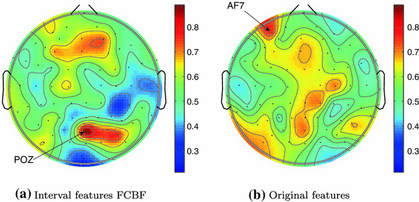
Approximation of the classification accuracy across the electrodes on the scalp for the Face/Car data (Experiment 1)

References
Blankertz, B., Dornhege, G., Schafer, C., Krepki, R., Kohlmorgen, J., Muller, K.R., Kunzmann, V., Losch, F., Curio, G.: Boosting bit rates and error detection for the classification of fast-paced motor commands based on single-trial eeg analysis. IEEE Trans. Neural Rehabil. Eng. 11(2), 127–131 (2003)
Blankertz, B., Muller, K.R., Curio, G., Vaughan, T., Schalk, G., Wolpaw, J., Schlogl, A., Neuper, C., Pfurtscheller, G., Hinterberger, T., Schroder, M., Birbaumer, N.: The BCI competition 2003: Progress and perspectives in detection and discrimination of EEG single trials. IEEE Trans. Biomed. Eng. 51(6), 1044–1051 (2004)
Breiman, L.: Random forests. Mach. Learn. 45, 5–32 (2001)
Delorme, A., Sejnowski, T., Makeig, S.: Enhanced detection of artifacts in eeg data using higher-order statistics and independent component analysis. NeuroImage 34, 1443–1449 (2007)
Dering, B., Martin, C.D., Thierry, G.: Is the N170 peak of visual event-related brain potentials car-selective? NeuroReport 20, 902–906 (2009)
Frank, A.: Asuncion. UCI machine learning repository (2010)
Garrett, D., Peterson, D.A., Anderson, C.W., Thaut, M.H.: Comparison of linear, nonlinear, and feature selection methods for EEG signal classification. IEEE Trans. Neural Syst. Rehabil. Eng. 11, 141–144 (2003)
Hall, M., Frank, E., Holmes, G., Pfahringer, B., Reutemann, P., Witten, I.H.: The WEKA data mining software: an update. SIGKDD Explor. 11, 37–57 (2009)
Hyvärinen, A., Oja, E.: A fast fixed-point algorithm for independent component analysis. Neural Comp. 9(7), 1483–1492 (1997)
Jung, T., Makeig, S., Westerfield, M., Townsend, J., Courchesne, E., Sejnowski, T.: Analysis and visualization of single-trial event-related potentials. Hum. Brain Mapp. 14(3), 166–185 (2001)
Lai, C., Reinders, M.J.T., Wessels, L.: Random subspace method for multivariate feature selection. Pattern Recogn. Lett. 27(10), 1067–1076 (2006)
Li, J., Zhang, L.: Regularized tensor discriminant analysis for single trial EEG classification in BCI. Pattern Recogn. Lett. 31, 619–628 (2010)
Lin, H.T., Li, L.: Novel distance-based SVM kernels for infinite ensemble learning. In: Proceedings of the 12th International Conference on Neural Information Processing, ICONIP’05, pp. 761–766 (2005).
Lu, B.L., Shin, J., Ichikawa, M.: Massively parallel classification of single-trial EEG signals using a min-max modular neural network. IEEE Trans. Biomed. Eng. 51, 551–558 (2004)
Palaniappan, R., Ravi, K.: Improving visual evoked potential feature classification for person recognition using pca and normalization. Pattern Recogn. Lett. 27(7), 726–733 (2006)
Peters, B.O., Pfurtscheller, G., Flyvbjerg, H.: Automatic differentiation of multichannel EEG signals. IEEE Trans. Biomed. Eng. 48, 111–116 (2001)
Polikar, R., Topalis, A., Green, D., Kounios, J., Clark, C.M.: Comparative multiresolutionwavelet analysis of erp spectral bands using an ensemble of classifiers approach for early diagnosis of Alzheimer’s disease. Comput. Biol. Med. 37, 542–558 (2007)
Quian Quiroga, R., Garcia, H.: Single-trial event-related potentials with wavelet denoising. Clin. Neurophysiol. 114, 376–390 (2003)
Rodríguez, J.J., Alonso, C.J., Boström, H.: Boosting interval based literals. Intell. Data Anal. 5, 245–262 (2001)
Rodríguez, J.J., Alonso, C.J., Maestro, J.A.: Support vector machines of interval-based features for time series classification. Knowl. Based Syst. 18, 171–178 (2005)
Samar, V.J., Swartz, K.P., Raghuveer, M.R.: Multi-resolution analysis of event-related potentials by wavelet decomposition. Brain Cognition 27, 398–438 (1995)
Schaefer, R.S., Farquhar, J., Blokland, Y., Sadakata, M., Desain, P.: Name that tune: decoding music from the listening brain. Neuroimage 56(2), 849 (2011)
Shen, K.Q., Ong, C.J., Li, X.P., Hui, Z., Wilder-Smith, E.P.V.: A feature selection method for multilevel mental fatigue EEG classification. IEEE Trans. Biomed. Eng. 54, 1231–1237 (2007)
Snodgrass, J.G., Vanderwart, M.: A standardized set of 260 pictures: norms for name agreement, image agreement, familiarity, and visual complexity. J. Exp. Psychol. 6, 174–215 (1980)
Sun, S., Zhang, C., Lu, Y.: The random electrode selection ensemble for EEG signal classification. Pattern Recogn. 41, 1663–1675 (2008)
Sun, S., Zhang, C., Zhang, D.: An experimental evaluation of ensemble methods for EEG signal classification. Pattern Recogn. Lett. 28(15), 2157–2163 (2007)
Thierry, G., Martin, C.D., Downing, P., Pegna, A.J.: Controlling for interstimulus perceptual variance abolishes N170 face selectivity. Nat. Neurosci. 10, 505–511 (2007)
Trejo, L.J., Shensa, M.J.: inear and neural network models for predicting human signal detection performance from event-related potentials: a comparison of the wavelet transform with other feature extraction methods, pp. 153–161. Society for Computer Simulation, San Diego (1993)
Übeyli, E.D., Gler, I.: Features extracted by eigenvector methods for detecting variability of EEG signals. Pattern Recogn. Lett. 28(5), 592–603 (2007)
Yu, L., Liu, H.: Feature selection for high-dimensional data: A fast correlation-based filter solution. In: Proceedings of the 20th International Conference on Machine Learning (ICML2003). Washington, DC (2003)
Zhang, X.L., Begleiter, H., Porjesz, B., Wang, W., Litke, A.: Event related potentials during object recognition tasks. Brain Res. Bull. 38, 531–538 (1995)
Acknowledgments
The authors are grateful to Prof Guillaume Thierry and Dr Benjamin Dering from the School of Psychology, Bangor University, UK, for providing the first dataset used in this study and for the useful discussion and comments on an earlier version of this manuscript.
Author information
Authors and Affiliations
Corresponding author
Rights and permissions
About this article
Cite this article
Kuncheva, L.I., Rodríguez, J.J. Interval feature extraction for classification of event-related potentials (ERP) in EEG data analysis. Prog Artif Intell 2, 65–72 (2013). https://doi.org/10.1007/s13748-012-0037-3
Received:
Accepted:
Published:
Issue Date:
DOI: https://doi.org/10.1007/s13748-012-0037-3