A systematic evaluation of assumptions in centrality measures by empirical flow data

Abstract

When considering complex systems, identifying the most important actors is often of relevance. When the system is modeled as a network, centrality measures are used which assign each node a value due to its position in the network. It is often disregarded that they implicitly assume a network process flowing through a network, and also make assumptions of how the network process flows through the network. A node is then central with respect to this network process (Borgatti in Soc Netw 27(1):55–71, 2005, https://doi.org/10.1016/j.socnet.2004.11.008). It has been shown that real-world processes often do not fulfill these assumptions (Bockholt and Zweig, in Complex networks and their applications VIII, Springer, Cham, 2019, https://doi.org/10.1007/978-3-030-36683-4_7). In this work, we systematically investigate the impact of the measures’ assumptions by using four datasets of real-world processes. In order to do so, we introduce several variants of the betweenness and closeness centrality which, for each assumption, use either the assumed process model or the behavior of the real-world process. The results are twofold: on the one hand, for all measure variants and almost all datasets, we find that, in general, the standard centrality measures are quite robust against deviations in their process model. On the other hand, we observe a large variation of ranking positions of single nodes, even among the nodes ranked high by the standard measures. This has implications for the interpretability of results of those centrality measures. Since a mismatch of the behaviour of the real network process and the assumed process model does even affect the highly-ranked nodes, resulting rankings need to be interpreted with care.

1 Introduction

Networks have been proven to be a natural and convenient representation for many complex systems, thus, systems consisting of entities interacting with each other: entities are represented by nodes, and their interactions are represented by edges. An often occurring question in the analysis of those networks is: which node is the most important one due to its position in the network? This question has led to the notion of centrality. Since the first mention of structural centrality by Bavelas (1948), a large number of centrality measures, i.e., functions that assign a value of importance to each node based on the structure of the graph, have been proposed. The most well known are probably degree centrality (Nieminen 1974), closeness centrality (Freeman 1978), betweenness centrality (Freeman 1977; Anthonisse 1971), eigenvector centrality (Bonacich 1972) and Katz centrality (Katz 1953). An overview is provided by Koschützki et al. (2005).

Although all those centrality measures solely use the structure of the graph, as it is required for structural indices (Sabidussi 1966), they all implicitly assume the presence of a process flowing through the network. This is already stated by Freeman (1977) for betweenness-based centrality measures: “Thus, the use of these three measures is appropriate only in networks where betweenness may be viewed as important in its potential for impact on the process being examined. Their use seems natural in the study of communication networks where the potential for control of communication by individual points may be substantively relevant.”

Borgatti (2005) made an important contribution by arguing that centrality measures do contain not only the assumption about the presence of a network process, but also assumptions about the properties of the process. In other words, each centrality measure incorporates a model of a flow process with certain properties. He identified two categories by which those process models differ: node-to-node transmission mechanism and the type of used trajectories. For the latter, he differentiates between shortest paths, paths (not necessarily shortest, but nodes and edges can only occur at most once in it), trails (edges might occur several times in it), and walks (in which nodes and edges might occur several times). For the mechanism of node-to-node transmission, Borgatti (2005) differentiates between transfer processes (an indivisible item is passed from node to node, such as physical goods) and duplication processes (the process entity is passed to the next node while also staying at the current node, such as information or infections).

Consider betweenness centrality as an example. For a node v, its betweenness centrality is defined as

$$\begin{aligned} B(v) = \sum _{\begin{array}{c} s \in V,\\ s\ne v \end{array}}{ \sum _{\begin{array}{c} t \in V,\\ s \ne t \ne v \end{array}}{ \frac{\sigma _{st}(v)}{\sigma _{st}}}} \end{aligned}$$

(1)

where $\sigma _{st}$ denotes the number of shortest paths from node s to node t and $\sigma _{st}(v)$ the number of those containing node v. Borgatti (2005) points out that the model of process flow contained in the betweenness centrality only uses shortest paths (since only those are counted), and is a transfer process (since one process entity can only use one shortest path and not several simultaneously). He furthermore points out that the measure considers an equal amount of flow between each pair of nodes since each node pair contributes a value between 0 and 1 to the overall measure value.

As a consequence, a centrality measure can only give interpretable results if the specific process matches with its assumed properties: Applying betweenness centrality in order to determine a node’s importance for an information spreading process will yield uninterpretable results.

When examining the widely used centrality measures, such as degree, closeness, and betweenness centrality, for their assumptions about the process properties, Borgatti (2005) finds that they are only appropriate for processes using shortest paths or for processes with a parallel duplication mechanism. It is clear that most processes which might be of interest are not of these types. For this reason, many adaptions of the classic centrality measures have been proposed: Freeman et al. (1991) proposed a betweenness centrality based on maximal flow, Newman (2005) one based on random walks instead of shortest paths, Stephenson and Zelen (1989) propose a betweenness centrality which includes all paths (not only shortest) between the pairs of nodes, for only naming a few examples.

Fig. 1

Extract from Wiki trajectories: all observed human navigations from Train to Apple. The extract contains all nodes which are contained in any trajectory from Train to Apple or in any shortest path from those nodes to the target node Apple. Nodes contained in any of the trajectories are colored black, the other grey. The nodes are grouped by their distance to the target node Apple

Our approach is different: instead of incorporating a different process model into the centrality measures, we use datasets of real-world network flows and incorporate the real-world information into the centrality measure. This approach enables us to analyze the impact of the assumptions on the centrality measure values:

• 1. Does it matter that real-world processes do not fulfill the assumptions that classic centrality measures contain about them?

• 2. Which assumptions do matter and which do not?

• 3. If there are nodes whose centrality value changes considerably, can we explain this effect?

Let us give a small motivating example for this approach: Sect. 6 will introduce a dataset containing trajectories of humans navigating through the Wikipedia article network by following the hyperlinks in the articles (the dataset was provided by West and Leskovec (2012)). The humans are playing a game in which they aim at navigating from a given start article to a given target article within as least clicks as possible. The resulting trajectories, humans moving from node to node by using the edges as fast as possible, actually constitute a network flow which–in theory–comes close to a flow assumed by the betweenness centrality: a set of indivisible entities who aim at using shortest paths between their start and end node.

Figure 1 shows a small example from this dataset, namely all (five) observed human navigation paths from the node Train to the node Apple. Included in the figure are all nodes which were used by any of the navigation paths or are included in any shortest path from Train to Apple, or in a shortest path from an used node to the node Apple. For a clearer presentation, edges which are not used by any of the considered navigation paths and which do not decrease the distance to the node Apple are removed. The nodes are grouped by their distance to the target node Apple: it can be reached from the start node Train within 3 links, for example by taking the path Train $\rightarrow$ Horse $\rightarrow$ Scientific classification $\rightarrow$ Apple. The five actually taken trajectories by the humans are shown by colored edges. Although this is only a tiny extract of the whole dataset, it can serve as an illustrative example. We observe that none of the navigation paths reaches the target node within the optimal number of steps, and thus, none of the optimal paths is actually used by the humans. Furthermore, there are nodes and edges which are used more frequently in the navigation paths than others. This is true for nodes and edges which are on an optimal paths as well as for nodes and edges which are not on any optimal path: while the node Food is not on any optimal path between Train and Apple, it is included in all five considered trajectories, several nodes on optimal paths, such as Scientific classification, are not included in any observed trajectory.

The example illustrates that also network flows for which the assumptions of transfer mechanism and shortest paths might be expected, can exhibit a different behaviour by real-world data. When applying a centrality measure on a network which assumes the network process using shortest paths, it is questionable whether it is able to identify the most important node with respect to the actual process taking place on the network.

Consider a second example depicted in Fig. 2: It shows a simple undirected network where two exemplary network flows are sketched by colored edges. Consider first the example network flow sketched by blue edges. Note that the network flow is directed although the network is undirected. The flow depicted by blue edges starts in the left subgraph and ends in the right subgraph, though it does not use the shortest path between them, but a detour instead. The standard betweenness centrality would assign high values to the nodes A and B since they are contained in (almost) all shortest paths between the left and right subgraph. If, however, the actual network flow (here depicted by blue edges) does not use shortest paths, standard betweenness centrality cannot recognize the most important node with respect to the actual network flow. A different case occurs for the network flow sketched by orange edges. This network flow does use shortest paths, but it is only relevant for the right subgraph. Standard betweenness centrality expects an equal amount of flow between each pair of nodes. If the actual network flow is only relevant for a small subset of nodes, the standard betweenness centrality does not identify the most important nodes with respect to the network flow at hand.

Fig. 2

An exemplary network with a simple network flow illustrated by colored edges. Standard betweenness centrality would assign a high value to the nodes A and B because their position is between the two larger subgraphs and all shortest paths between the subgraphs contain the nodes A and B. If, however, an exemplary network flow such as the one sketched by blue edges, does not use those edges, standard betweenness centrality is not able to identify the most important node with respect to the existing network flow

The main goal of this work is to find out whether those statements are only true for the shown toy examples, but also for real-world examples. For this purpose, we introduce flow-based centrality variants which partly use the simple process model contained in the standard centrality measure, and partly use the real-world information. The different variants can be thought of switching on and off the different assumptions of the process model, for example, one variant keeps the assumption of shortest paths, but does not keep the assumption of equal amount of flow between all node pairs—instead it uses the actual amount of network flow contained in the real-world dataset. We perform this approach for the classic centrality measures closeness and betweenness and for four different datasets of real-world network flows. It is clear that our newly introduced flow-based centrality measures are no centrality measures in the strict sense: they actually use more information than the network structure. However, we actually do not aim at introducing new centrality measures, but aim to investigate to which extent the existing centrality measures are robust against perturbations in their process model. Informally speaking, how much do the results of centrality measures change if certain assumptions of them are replaced by real-world flow properties?

Preliminary results with a similar approach only concerning the betweenness centrality have been published in Bockholt and Zweig (2018). In this work, the approach is extended to other types of centralities, and a detailed analysis explaining the changes of rankings is provided.

This work is structured as follows: Sect. 2 introduces necessary definitions and notations as well as formal definitions of the classic centrality measures. Section 3 reviews existing studies and contributions relevant for our work. Section 4 discusses the assumptions of the introduced centrality measures in details and also points to previous empirical results of real-world network processes–to which extent they fulfill the common assumptions. Section 5 introduces flow-based closeness and betweenness variants. Section 6 introduces the used datasets of real-world network processes. For all data sets, all flow-based closeness and betweenness variants as well as the standard centrality measures are computed. The results are described in Sects. 7 and 8, structured by the questions:

• 1. How robust are the standard centrality measures against deviations in their process model? Section 7 therefore compares the rankings of the flow-based centrality measures with the rankings of the corresponding standard centrality measure.

• 2. For which reason do certain nodes gain importance or drop in importance? Section 8 focuses on the nodes which are ranked high by any of the centrality measures and explains why some nodes gain or lose importance significantly for some measure variant.

Section 9 concludes the article with a summary of the main results and an outlook to possible future work.

2 Definitions

2.1 Graph definitions

Let $G=(V,E,\omega )$ be a directed simple weighted graph with a vertex set V, an edge set $E\subseteq V \times V$ and a weight function $\omega :E \rightarrow \mathbb {R}^+$ that assigns positive weights to the edges. A walk is an alternating (finite) sequence of nodes and edges, $P = (v_1, e_1, v_2, \dots , e_{k-1}, v_k)$ with $v_i \in V$ and $e_j = (v_j,v_{j+1}) \in E$ for all $i \in \{1, \dots , k\}$ and $j \in \{1, \dots , k-1\}$, respectively. If the edges are pairwise distinct, P is called a trail. If nodes and edges of P are pairwise distinct, P is called a path. Since we only consider simple graphs, P is uniquely determined by its node sequence and the notation can be simplified to $P = (v_1, v_2, \dots , v_k)$. The length of a walk P is denoted as |P| and is defined as $|P| = \sum _{i=1}^{k-1}\omega (e_i)$. The start node of the path P is denoted as $s(P) = v_0$, the end node as $t(P) = v_k$. If a node v is contained in a walk P, we write $v\in P$.

In graph G, let d(v, w) denote the length of the shortest path from node v to node w. If w cannot be reached from v, we set $d(v,w) := \infty$.

Section 6 will introduce datasets containing real-world network flows where the trajectory of each process entity can be modeled as walk in the graph. We will denote the set of (actually taken) walks in G by $\mathcal {P} = \{P_1, \dots , P_{\ell }\}$. In order to distinguish between actually taken walks contained in the dataset and possible walks in the graph, we will use the term trajectory for an actually taken walk.

2.2 Centrality measures

In general, a centrality measure is a function $c:V\rightarrow \mathbb {R}$ which assigns a value to each node. Normally, a high value of c(v) indicates a great importance of node v in the graph.

Closeness centrality The closeness centrality measures the average distance of a node v to all other nodes.

A common motivating example for closeness-like centrality measures is a facility location problem: for a given environment, a facility is to be placed such that the total distance from all other places to it is minimal. In his original work, Freeman (1977) defined the closeness centrality as

$$\begin{aligned} C(v)=\frac{|V|-1}{\sum _{w\in V}d(w,v)}, \end{aligned}$$

the inverse of the average distance from all other nodes to v. A node is considered as central if the average distance to all other nodes is small, i.e., all other nodes can reach v quite fast–on average.

However, if there are nodes $v,w \in V$ for which there does not exist any path between them, computing the closeness centrality by the above formula is problematic which is why we use the following common adaption:

$$\begin{aligned} C^{\leftarrow }(v)=\sum _{w\ne v \in V}\frac{|V|-1}{d(w,v)} \end{aligned}$$

(2)

with the convention $\frac{1}{\infty }=0$.

If the graph is directed, it makes a difference whether the distance from or to a node is considered. Therefore, depending on the use case, another common variant of the closeness centrality is

$$\begin{aligned} C^{\rightarrow }=\sum _{w\ne v \in V}\frac{|V|-1}{d(v,w)}. \end{aligned}$$

(3)

We will refer to the former as out-closeness $C^{\rightarrow }$ and to the latter as in-closeness $C^{\leftarrow }$.

Betweenness centrality Betweenness centrality was introduced by Freeman (1977) (independently proposed by Anthonisse (1971) as rush in a never published work) and is supposed to measure to which extent a node v lies “between” the other nodes. The common motivation is the identification of so-called gatekeeper nodes which are able—due to their position—to control the flow between the other nodes. For this purpose, for each node pair $s,t \in V$, it is counted how many shortest paths exist from s to t and how many of them contain node v. Formally, let $\sigma _{st}$ denote the number of shortest paths from s to t where $\sigma _{st}=1$ if $s=t$. For a node $v, \sigma _{st}(v)$ denotes the number of shortest paths from s to t that pass through v. The betweenness centrality for a node v is then defined as

$$\begin{aligned} B(v) = \sum _{\begin{array}{c} s \in V,\\ s\ne v \end{array}}{ \sum _{\begin{array}{c} t \in V,\\ s \ne t \ne v \end{array}}{ \frac{\sigma _{st}(v)}{\sigma _{st}}}}. \end{aligned}$$

(4)

3 Related work

The concept of centrality in graphs is already known for several decades. It was originally introduced by Bavelas (1948) for human communication networks. In the following decades, a large number of different centrality indices emerged, each suited for a specific application scenario in mind (see Koschützki et al. 2005 for an overview of the most common centrality indices). Based on the work of Freeman (1978), the three classic centrality measures are still degree, closeness, and betweenness centrality, additionally to Eigenvector centrality (Bonacich 1972), Katz centrality Katz (1953) or Google’s PageRank centrality (Page et al. 1999). A recent contribution to this field has been made by Schoch and Brandes (2016) proposing a unifying framework of centrality indices based on path algebras.

Borgatti (2005) points out that those centrality measures are all tied to a process flowing through the network, most of them assuming that the process uses shortest paths. It is obvious that this assumption is not necessarily true for many relevant processes. For this reason, several variants of the classic centrality measures have been proposed which either relax the restriction of shortest paths or incorporate a different process model into the measure.

Freeman et al. (1991) suggested a flow-betweenness centrality which is based on the idea of maximum flow between all pairs of nodes. In this model, edges of the graph can be understood as pipes with a capacity and instead of counting the (proportion of) shortest paths through a node v, the maximum possible flow passing through v is considered for the flow betweenness centrality. This implies that the flow betweenness centrality also integrates the contribution of non-shortest paths. However, Newman (2005) argues that flow betweenness centrality yields unintuitive results since in realistic situations, the process of interest usually does not take any ideal path from a source to a target (which is still an assumption of the flow betweenness centrality because it is assumed that information travel on ideal paths in the sense of maximum flow). Newman (2005) notes that “in most cases a realistic betweenness measure should include non-geodesic paths in addition to geodesic ones” which is why he introduces a betweenness centrality based on random walks through the network. The idea of developing a centrality measure based on random walks through the network existed before, though. Bonacich (1987) proposed the power centrality which measures the expected number of times that a random walk with a fixed probability of stopping in each step, passes through a node, averaged over all possible starting points for this walk. The random walk centrality introduced by Noh and Rieger (2004) and the information centrality from Stephenson and Zelen (1989) are also based on random walks on the network and can be seen as the “random-walk version of closeness centrality” (Newman 2005).

Other variants—just naming a few—allow to incorporate both, shortest paths and paths up to a certain length (Borgatti and Everett 2006); or even all possible walks, weighted inversely by their length (Borgatti and Everett 2006). Dolev et al. (2010) propose a generalized variant of flow betweenness centrality incorporating flows generated by arbitrary routing strategies.

Systematically incorporating real-world process information into centrality measures has—to our best knowledge—not been done before. Meiss et al. (2008) use the recorded user traffic in the Web to rank single pages by their importance. They use the real user traffic to validate the random surfer model contained in the PageRank algorithm and analyze for which assumptions of the random surfer behaviour the real users’ behaviour differs. Dorn et al. (2012) use the passenger flow data in the US air transportation network to introduce a stress betweenness centrality counting on how many passenger journeys an airport is contained in and compare the resulting rankings to rankings of the standard betweenness centrality. They find that the results significantly change when the centrality considers the number of actually taken paths instead of all possible shortest paths.

Ghosh and Lerman (2012) make a connection between Borgatti’s work and the centrality measures PageRank and Alpha Centrality. Since PageRank assumes a transfer process (which they call conservative process) and Alpha Centrality assumes a parallel duplication process (which they call a non-conservative process), they test this assumption on two real-world datasets. They use two datasets containing a non-conservative process, and can show that for them, Alpha Centrality assuming a non-conservative process yields better results than PageRank which assumes a conservative process.

Real-world process information, however, has been used before to infer other kind of knowledge about the network or the system. West et al. (2009) used human trajectories through the Wikipedia network (as in the introductory example) for deducing a semantic similarity between the articles. Rosvall et al. (2014) developed a method for deriving communities by the network’s usage pattern. Weng et al. (2013) use the pattern of information diffusion as a predictor for future network evolution, i.e., the formation of new edges. GPS trajectories of travelers or taxis have been used to identify popular places (Zheng et al. 2009) or to compute the effectively quickest route between places (Yuan et al. 2010).

4 Assumptions of centrality measures

All introduced centrality measures are somehow based on paths or walks in the graph (Borgatti and Everett 2006): degree centrality counts paths of length 1 from node v, closeness centrality is based on the length of the shortest paths from v to the other nodes, while the betweenness centrality counts the number of shortest paths through node v. This implies that something is flowing through the network and uses these paths. A node central with respect to one of the centrality measures is then only central with respect to the network flow (Borgatti 2005; Zweig 2016). As already introduced in Sect. 1, all centrality measures do not only contain the assumption about the existence of a network flow, but also about the properties of the flow process (Borgatti 2005) which we will review for the introduced measures in the following.

• Flowing on shortest paths All introduced measures consider shortest paths, assuming that whatever flows through the network uses shortest paths. This also implies that the flow actually has a target to reach (and knows how to reach this target). This is certainly not true for all network flows of interest.

• Parallel usage of paths (Borgatti 2005) differentiates different mechanisms of node-to-node transmissions concerning how the network flow moves through the network: by a transfer mechanism, by serial or by parallel duplication. In a network flow with a transfer mechanism, indivisible items actually move from node to node, while for network flows with duplication mechanisms, the flow is copied to the next node as for example the spreading of an infection. This duplication mechanism can happen in serial (one neighbor at a time) or in parallel (all neighbor nodes at once). Since closeness centrality counts the length of the shortest paths, it is meaningful to apply for networks where the network flow uses shortest paths or diffuses via parallel duplication where all possible paths are taken in parallel (Borgatti 2005). This does not hold for betweenness centrality: this measure assumes that the network flow uses shortest paths, but moves via a transfer mechanism and hence can only use one shortest path at a time.

• Equal amount of flow between any node pair Due to the calculation of the centrality values, each pair of nodes contributes to the value: for the closeness centrality, it is assumed that there exists flow from all other nodes w to v where each pair (w, v) contributes its distance to the measure. For the betweenness centrality of node v, it is assumed that there is a flow between any two nodes s and s where each node pair (s, t) can contribute a value between 0 and 1 to the centrality value of v. In both cases, it is assumed that (i) there exists a flow between any node pair, and (ii) the flow between the node pairs is equally important. This is certainly not true for many real-world processes.

• Graph distance is meaningful Closeness centrality incorporating the graph distances between nodes in the calculation contains the assumption that graph distance is actually a meaningful concept for the network and network flow. In networks serving as infrastructure for transportation flows for example, such as road networks and humans traveling from one place to another, distances of 10 km or 1000 km do have different qualities. In other networks, however, it might not be the case: Friedkin (1983) described a so-called horizon of observability in communication networks, a distance beyond which members of the network are not aware of each other. Depending on the concrete network flow, it is possible that a distance of 10 or 1000 is actually of the same quality, if they lie both beyond the horizon distance.

• All edges are available When computing shortest paths or any variant of random walks for a centrality measure on a static network, an essential assumption is taken for granted: the permanent availability of all edges. This assumption is not given in temporal networks where edges have a timestamp because the corresponding connection in the system is only available at certain points in time. Scholtes et al. (2016) proposed temporal variations of centrality measures which only incorporate time-respecting paths, i.e., paths in which the order of the contained edges respects their timing order.

While it might be true for many processes that they have a target that they try to reach as fast as possible, it is not necessarily true that they actually use shortest paths. One example is human navigation in networks which exists in two variants: in the first, a human needs to navigate in a complex network by physically or virtually moving from node to node; in the second, some item has to reach a target in a social network while it is forwarded by each node individually—by only having a local view on the network structure. A famous example of the latter setting is the small-world experiment by Milgram (1967) in the late 1960s. In this experiment, Milgram asked randomly selected people to send a letter to a target person by forwarding it to their own personal contacts—who then would repeat this, until the letter eventually reaches the target person. Although the structure of the underlying social network is not known to the involved persons, the letters reached the target person within five intermediate stations.¹ This type of experiment has been repeated on a larger scale: The experiment conducted by Dodds (2003) involved more than 60,000 users who were asked to forward an email to their acquaintances in order to reach one of 18 target persons.

For the other variant of human navigation in networks where the human themselves travel through the network, there has been a lot of evidence that humans are surprisingly efficient in finding short paths—they are, however, rarely optimal. Sudarshan Iyengar et al. (2012) and Gulyás et al. (2020) investigated human paths in a word morph game: a player is given two English words, and the player needs to transform the first word into the second word by substituting single letters while intermediate words need to be existing English words. The player’s sequence can be seen as a walk through the word network where there is an edge between two existing words if their Hamming distance is exactly one. Sudarshan Iyengar et al. (2012) found that the players’ solutions are in average 1.7 times longer than the shortest path between the words. When considering only the solutions of experienced players, the solutions’ length even decreases to 1.1–1.2 times the optimal solution length (Gulyás et al. 2020).

This observation is supported by the results of West and Leskovec (2012) who analyzed human paths through the Wikipedia article network where a node represents a Wikipedia article and there is an edge from one node to another if there is a link from the one article pointing to the other article. In an online-based experiment, West asked his participants to navigate through this network by giving them a source and a target article. He was able to collect more than 30,000 paths and could show that human wayfinding in this network is surprisingly efficient (albeit not optimal) although the complete structure of the network is not known to the participants.

This finding also holds for humans moving in physical environments: Zhu and Levinson (2015) considered human travel patterns within cities and found that they do use short paths, but no shortest paths, Manley et al. (2015) analyzed trajectories of minicabs in London and found a preference of anchor-based routes: it seems that drivers select certain locations as landmarks and use those for constructing their route. This yields short, but non-optimal paths. Also for non-human transfer processes, studies have found similar results: Gao and Wang (2002) show that also routes of packages in the Internet involve non-shortest paths due to routing strategies, Csoma et al. (2017) provide a comparative analysis of paths of different domains pointing to the same direction.

In recent work, we have shown that several real-world processes do not satisfy the assumption of equal amount of flow (Bockholt and Zweig 2019): we have shown that there are few hub nodes and edges which are used heavily by the process, while the majority of the nodes is visited at most once by the process. The same holds for node pairs: a few node pairs are the source and target of many process entities, while there is no real flow between many node pairs.

5 Flow-based centrality measures

The question arises whether it actually matters that the assumptions of the centrality measures are not met. For investigating this question, we present the following approach: For each of the centrality measures, we introduce flow-based variants which—instead of theoretically existing shortest paths in the graph—incorporate the observed walks of real-world processes. By introducing different variants, we are able to “switch on or off” the different assumptions and replace them by the properties of the real-world process. Our goal is not to introduce further centrality measures, but to investigate to which extent the included assumptions have an impact on the results if they are not met.

5.1 Flow-based betweenness measures

The following four variants of flow-based betweenness measures have been proposed in Bockholt and Zweig (2018), and their definitions are given here again since they are needed in the following.

As a general framework for introduced flow-based betweenness measures, we introduce a weighted betweenness centrality by

$$\begin{aligned} B_{w}(v) = \sum _{s\in V}\sum _{t\in V} w(s,t,v)\cdot \frac{\sigma _{st}(v)}{\sigma _{st}} \end{aligned}$$

(5)

with a weight function $w:V\times V\times V \rightarrow \mathbb {R}$. The standard betweenness centrality introduced in Sect. 2 is obtained by inserting the weight function $w(s,t,v)=0$ if $s=t$ or $s=v$ or $v=t$, and $w(s,t,v)=1$ otherwise.

We will introduce four variants of flow-based betweenness measures (for an overview, see Table 1): two will keep the assumption of shortest paths (indicated by a subscripted S vs. a subscripted R when real trajectories are incorporated), and two will keep the assumption of equal amount of flow between any node pair (a subscripted W will indicate that the real amount of flow is incorporated in the weight function).

For all variants, a set of observed trajectories by the real-world process, denoted by $\mathcal {P}=\{P_1, P_2, \dots , P_{\ell }\}$, is used (Fig. 3).

Table 1 Categorization of the introduced flow-based betweenness centralities

Fig. 3

Application of the flow-based betweenness measures on an example graph with the set $\mathcal {P}=\{{P_1}, {P_2}, {P_3}, {P_4}, {P_5}, {P_6}\}$ with ${P_1} = (10,1,2,3,4,6), {P_2} = (7,3,4,6), {P_3} = (8,7,2,3,9,4,6), {P_4} = (7,3,9,4,6)$, ${P_5} = (1,2,3,9,4)$, and ${P_6} = (7,2,3,9,4,6)$. Size and color of the nodes correspond to their centrality value, and the values of the centrality measures are shown in the grey box next to each node

Betweenness variant $B_S$ Keeping the assumption that the process is flowing on shortest paths, this variant will only count (shortest) paths between node pairs for which there is real-world flow. Consider again Fig. 2 as a motivating example. Standard betweenness centrality would assign the highest value to nodes A and B because it lies on (almost) all shortest paths between the left and the right node group. However, assume that a real-world process only flows within the two groups, such as the orange flow in the figure. Then, there is no reason why nodes A and B would be assigned an important role as mediator or “gatekeeper” between the two groups. Therefore, the present variant will only count shortest paths between nodes s and t for which there is a real-process trajectory from s to t. We define

$$\begin{aligned} B_S(v) = \sum _{s\in V}\sum _{t\in V} w_S(s,t,v)\cdot \frac{\sigma _{st}(v)}{\sigma _{st}} \end{aligned}$$

(6)

with the weight function

$$\begin{aligned} w_S(s,t,v) = {\left\{ \begin{array}{ll} 1 &{} \text {if }\exists P \in \mathcal {P}: s(P)=s \text { and }t(P)=t \\ 0 &{} \text { otherwise} \end{array}\right. } \end{aligned}$$

Betweenness variant $B_{SW}$ In this variant, the assumption that the process is flowing on shortest paths is kept, but the assumption of equal amount of flow is dropped. The idea is that a node will be assigned a higher value if it is on many shortest paths between highly demanded node pairs than a node on many shortest paths between node pairs which are never used as source and target. The weight function will hence be proportional to the number of real-process paths starting and ending in those node pairs. We define

$$\begin{aligned} B_{SW}(v) = \sum _{s \in V}\sum _{t \in V} w_{SW} \cdot \frac{\sigma _{st}(v)}{\sigma _{st}} \end{aligned}$$

(7)

with the weight function

$$\begin{aligned} w_{SW}(s,t,v) = |\{P \in \mathcal {P}| s(P)=s, t(P)=t\}| \end{aligned}$$

Note that this measure might still yield low values for nodes contained in many observed trajectories, if they are not on the shortest path between the highly demanded node pairs.

Betweenness variant $B_R$ Unlike the previous two measure variants which are counting in how many shortest path a node v is contained, the following two variants will count in how many observed trajectories a node is contained. A motivating example can been seen in Fig. 2: assume there is a real process flow between the two groups, such as the one depicted by blue edges, but all process entities use the path via nodes C, D and E and not the shortest path via nodes A and B. Standard betweenness centrality would assign nodes A and B the highest values, the following variant counting the real paths would assign a higher value to nodes C, D and E than to nodes A and B. For this reason, we define a flow-based variant of $\sigma _{st}$ and $\sigma _{st}(v)$ counting the number of real trajectories from s to t (containing v). Since we want to keep the assumption of equal amount of flow between all node pairs as much as possible, we define $\sigma ^{\mathcal {P}}_{\cdot st\cdot }$ as the number of paths $P \in \mathcal {P}$ containing s and t. Otherwise, if $\sigma ^{\mathcal {P}}_{\cdot st\cdot }$ was defined as the number of paths P from s to t, node pairs which are not start and end node of any real process trajectory will not contribute to the centrality measure, and the assumption of equal amount of flow would already been dropped. It is clear that also with the introduced definition of $\sigma ^{\mathcal {P}}_{\cdot st\cdot }$, not all node pairs will contribute, since not for all node pairs, there will a exist a real trajectory containing both nodes. But this is the best we can do. We hence define

$$\begin{aligned} B_R(v) = \sum _{s\in V}\sum _{t \in V} w_R \cdot \frac{\sigma ^{\mathcal {P}}_{\cdot st\cdot }(v)}{\sigma ^{\mathcal {P}}_{\cdot st\cdot }} \end{aligned}$$

(8)

with the weight function $w_R(s,t,v) = 1$ for all $s,t,v \in V$ with $s\ne t$ and also here the convention $\frac{0}{0} = 0$.

Betweenness variant $B_{RW}$ The last measure variant drops both the assumption of shortest paths (by counting observed trajectories) and the assumption of equal amount of flow between all node pairs (by introducing a weight function proportional to the number of observed trajectories from s to t). In this case, since the weight function will yield 0 for node pairs between which there is no real process flow, a flow-based version of $\sigma _{st}$ can be used which counts the real process trajectories from s to t: $\sigma _{st}^{\mathcal {P}} = |\{P \in \mathcal {P}|s(P)=s, t(P)=P\}|$. With this (and the corresponding definition for $\sigma _{st}^{\mathcal {P}}(v)$), we define

$$\begin{aligned} B_{RW}(v)&= \sum _{s\in V}\sum _{t \in V}w_{WR}\cdot \frac{\sigma _{st}^{\mathcal {P}}(v)}{\sigma _{st}^{\mathcal {P}}} \end{aligned}$$

(9)

$$\begin{aligned}&= |\{P \in \mathcal {P}|v \in P\}| \end{aligned}$$

(10)

with the weight function

$$\begin{aligned} w_{RW}(s,t,v)&=w_{SW}(s,t,v)\\&=|\{P \in \mathcal {P}| s(P)=s, t(P)=t\}|. \end{aligned}$$

This yields a sort of stress betweenness centrality since it simply counts the number of process trajectories a node v is contained in (at least once).

5.2 Flow-based closeness measures

For the closeness centrality, similar assumptions than for the betweenness centrality are included: the process is using shortest paths, and there is an equal amount of flow to (from) each node v from (to) all other nodes. In order to derive closeness variants which drop or keep those assumptions separately, we introduce also here a generalized closeness centrality as framework. For a better readability, we will introduce the variants as in-closeness, the corresponding out-closeness can be easily derived in the same way. Let

$$\begin{aligned} C_{\omega }(v) = \sum _{w\in V(v)}\frac{N(v)}{\omega (w,v)\delta (w,v)} \end{aligned}$$

(11)

be a generalized weighted closeness centrality with a weight function $\omega :V\times V \rightarrow \mathbb {R}$, a normalization factor $N: V \rightarrow \mathbb {N}$, a distance function $\delta :V\times V \rightarrow \mathbb {R}$, and v-based subset of nodes.

By inserting $N(v)=|V|-1$ for all $v \in V, \delta (v,w)=d(v,w)$, $\omega (v,w) = 1$ for all $v,w \in V$, and $V(v):=V\setminus \{v\}$, the standard (in-)closeness centrality can be derived.

As in the previous section where the flow-based betweenness variants were introduced, the following closeness variants can also keep or drop the assumption of shortest paths (indicated by a subscripted S or R), and keep or drop the assumption of equal amount of flow (indicated by a subscripted W if weights are proportional to the actual number of real paths). For an overview of the variants, see Table 2.

In the following, when introducing closeness variants or illustrating properties, we will use the in-closeness as example for a better readability.

Table 2 Categorization of the introduced flow-based (out-)closeness centralities

Fig. 4

Application of the flow-based closeness (out-)measures on an example graph with the set $\mathcal {P}=\{{P_1}, {P_2}, {P_3}, {P_4}, {P_5}, {P_6}\}$ with ${P_1} = (10,1,2,3,4,6), {P_2} = (7,3,4,6), {P_3} = (8,7,2,3,9,4,6), {P_4} = (7,3,9,4,6), {P_5} = (1,2,3,9,4)$, and ${P_6} = (7,2,3,9,4,6)$. Size and color of the nodes correspond to their centrality value, and the values of the centrality measures are shown in the grey box next to each node. Only out-variants are shown here

Closeness variant $C_S$ In the first variant, the assumption of shortest paths is kept while only distances between those nodes are considered between which there is a real process flow. We hence define

$$\begin{aligned} C^{\leftarrow }_{S}(v) = \sum _{w \in V_S(v)}\frac{N_S(v)}{\omega _S(w,v)d(w,v)} \end{aligned}$$

(12)

with the weight function

$$\begin{aligned} \omega _S(w,v) = {\left\{ \begin{array}{ll} 1&{} \text {if }\exists P \in \mathcal {P}: s(P)=w, t(P)=v\\ 0&{} \text {otherwise} \end{array}\right. } \end{aligned}$$

Furthermore, the normalization factor is defined as

$$\begin{aligned} N_S(v)=|\{w\in V | \exists P \in \mathcal {P}: s(P)=w, t(P)=v\}| \end{aligned}$$

and $V_S(v)=\{w \in V|\omega _S(w,v)\ne 0\}$. In other words, for calculating $C^{\leftarrow }_S(v)$, we consider the shortest distances from all nodes w to v for which there exists a observed trajectory starting in w and ending in v.

Closeness variant $C_{S'}$ The previous variant is very restrictive: only the distance from those nodes w are considered for which there is a observed trajectory starting in w and ending in v. This implies that all nodes that are not the end node of any node are not assigned any closeness value. In order to relax this restriction, we introduce the variant $C_{S'}$ where the distances from all nodes w to node v are considered which are contained in the same real trajectory: We define

$$\begin{aligned} C^{\leftarrow }_{S'}(v) = \sum _{w\in V_{S'}(v)}\frac{N_{S'(v)}}{\omega _{S'}(w,v)d(w,v)} \end{aligned}$$

(13)

with the weight function

$$\begin{aligned} \omega _{S'}(w,v) = {\left\{ \begin{array}{ll} 1 &{} \text { if } \exists P \in \mathcal {P}: P=(\dots , w\dots , v, \dots ), v \ne w\\ 0 &{} \text { otherwise} \end{array}\right. } \end{aligned}$$

and the normalization factor

$$N_{S'}(v) = |\{w \in V \mid \exists P\in \mathcal {P}: P=(\dots , w\dots , v, \dots ), v\ne w\}|$$

and the node subset $V_{S'}(v) = \{w \in V| w\ne v, \omega _{S'}(w,v)\ne 0\}$.

It is clear that all intermediate nodes between any w and v will also contribute to the centrality value, similarly to the standard closeness centrality. Also similarly to the standard closeness centrality, the node itself does not contribute to its own centrality value.

Closeness variant $C_{SW}$

Like the previous variant, this variant also considers the length of the shortest paths, but paths between node pairs which are used often by the real process contribute more to the centrality value. Hence, the weight function is proportional to the number of real process trajectories from w to v. The closeness variant is then defined as

$$\begin{aligned} C_{SW}^{\leftarrow }(v) = \sum _{w\in V_{SW}(v)}\frac{N_{SW}(v)}{\omega _{SW}(w,v)d(w,v)} \end{aligned}$$

(14)

with

$$\begin{aligned} \omega _{SW}(w,v) = |\{P \in \mathcal {P}| P=(\dots ,w,\dots ,v,\dots )\}| \end{aligned}$$

and the normalization factor

$$\begin{aligned} N(v) = \sum _{w \in V}\omega _{SW}(w,v) \end{aligned}$$

and $V_{SW}(v) = \{w \in V|w\ne v, \omega _{SW}(w,v)\ne 0\}$.

Closeness variant $C_R$ In this and the following variants, the assumption of shortest paths is dropped, and instead, the “real” path length is considered. For this reason, we need to define a flow-based path length $d^{\mathcal {P}}(v,w)$. Since different observed process trajectories containing both v and w can take different paths of different lengths in order to reach w from v, those different “real” lengths need to be aggregated. We decided to average those, but also other aggregations might be plausible. Formally, for nodes $v,w\in V$ occurring in a real trajectory P, we define their P-distance $d^P(v,w)$ as the sum of the weights of the edges in P between the occurrence of v and w in P. The flow-based distance of two nodes is then the average over all occurrences of v before w in trajectories in $\mathcal {P}$. Consider the example shown in Fig. 4 with six real trajectories. For the nodes 3 and 6 with a graph distance of 2, we obtain the following P-distances $d^{{P_1}}(3,6)=2$, $d^{{P_2}}(3,6)=2, d^{{P_3}}(3,6)=3, d^{{P_4}}(3,6)=3$, $d^{{P_6}}(3,6)=3$, while $d^{{P_5}}(3,6)$ is not defined. By averaging those values, this yields an flow-based path length of $d^{\mathcal {P}}(3,6)=\frac{13}{5}=2.6$. The closeness variant is then defined as

$$\begin{aligned} C_{R}^{\leftarrow }(v) = \sum _{w\in V_R(v)}\frac{N_{R}(v)}{\omega _{R}(w,v)d^{\mathcal {P}}(w,v)} \end{aligned}$$

(15)

with

$$\begin{aligned} \omega _{R}(w,v) = {\left\{ \begin{array}{ll} 1 &{} \text { if } \exists P \in \mathcal {P}: P=(\dots ,w,\dots ,v,\dots ), v \ne w\\ 0 &{} \text { otherwise} \end{array}\right. } \end{aligned}$$

and

$$\begin{aligned} N_{R}(v) = |\{w \in V| \exists P \in \mathcal {P}: P=(\dots w\dots v\dots )\}| \end{aligned}$$

and $V_R(v) = \{w\in V|w\ne v, \omega _{R}(w,v)\ne 0\}$

Closeness variant $C_{RW}$ In analogy to the previous variants, we extend the previous variant by dropping the assumption of equal amount of flow and introducing a weight function proportional to the amount of flow from w to v. Then,

$$\begin{aligned} C_{RW}^{\leftarrow }(v) = \sum _{w\in V_{RW}(v)}\frac{N_{RW}(v)}{\omega _{RW}(w,v)d^{\mathcal {P}}(w,v)} \end{aligned}$$

(16)

with

$$\begin{aligned} \omega _{RW}(w,v) = |\{P \in \mathcal {P}| s(P)=w, t(P)=v\}| \end{aligned}$$

and the normalization factor

$$N_{RW}(v) = \sum _{w \in V}\omega _{RW}(w,v)$$

and $V_{RW}(v) = \{w\in V|w\ne v, \omega _{RW}(w,v)\ne 0\}$.

Closeness variant $C_{RW'}$

We again loosen the restriction of the previous variant by counting the distances of all nodes pairs which are both contained in at least one common observed trajectory instead of counting only distances between node pairs which are source and target of at least one observed trajectory. Then, we get

$$\begin{aligned} C_{RW'}^{\leftarrow }(v) = \sum _{w\in V_{RW'}(v)}\frac{N_{RW'}(v)}{\omega _{RW'}(w,v)d^{\mathcal {P}}(w,v)} \end{aligned}$$

(17)

with

$$\begin{aligned} \omega _{RW'}(w,v) = |\{P \in \mathcal {P}|v,w\in P, v\ne w\}|\} \end{aligned}$$

and

$$\begin{aligned} N_{RW'}(v) = \sum _{w\in V}\omega _{RW'}(w,v) \end{aligned}$$

and $V_{RW'}(v)=\{w \in V|w\ne v, \omega _{RW'}(w,v)\ne 0\}$.

For all introduced variants, the in-closeness was introduced, and the corresponding out-closeness can be derived easily.

6 Datasets

Datasets appropriate for testing the introduced flow-based centrality measures need to satisfy the following requirements

• 1. a process is flowing through the network by moving from node to node by using the underlying network structure

• 2. the process spreads through the network by actually moving from node to node, i.e., there is an entity which hops from node to node and that can only be present at one node in one moment in time,

• 3. the process does not spread randomly, but is moving through the network with a target, i.e., a pre-determined node to reach

We therefore used the datasets which are described in the following. Tables 3 and 4 show basic properties of the datasets used, Fig. 5 shows example trajectories for each dataset.

Fig. 5

Illustration of the datasets used. For each dataset, an example trajectory is shown

Table 3 Overview of the used datasets

Table 4 Properties of the used datasets. |V| and |E| denote the cardinality of node and edge set of the underlying graph, $|\mathcal {P}|$ the number of observed trajectories

• Airline transportation (DB1B) The US Bureau of Transportation Statistics publishes the Airline Origin and Destination Survey (DB1B) for every quarter year (RITA TransStat 2016). This database contains 10% of all airline tickets of passenger journeys within the USA (of all reporting carriers). We used the databases of the years 2010 and 2011 to extract passengers’ airline itineraries including start and destination airports as well as all intermediate stops. If an itinerary contains an outbound and return trip, the itinerary is split into two trips. We construct a network in the following way: A node again represents a city, and airports with the same Market City ID in the data are merged into one node; for example, the airports Chicago O’Hare International Airport and Chicago Midway International are both assigned to the city node of Chicago. We set a threshold for the insertion of nodes and edges: a node is only inserted in the network if it is contained in at least 100 passenger itineraries and an edge from v to w is inserted if the data contain at least 10 passenger itineraries with a flight from an airport in v to an airport in w. This procedure yields a network with 415 nodes. Since for almost all node pairs v, w, both edges (v, w) and (w, v) exist, the network is simplified to an undirected network where the undirected edge (v, w) is inserted if the directed edge (v, w) or the directed edge (w, v) exists. This yields a network with 5141 undirected edges.

• London Transport (LT) Transport of London, the governmental authority responsible for the public transport in the area of London yearly publishes the Rolling Origin and Destination Survey (Transport for London 2017), a 5% sample of all passengers’ journeys using an Oyster Ticket, an electronic ticket, in one week in November 2017. The database contains for each trip the station where the trip started and ended as well as stations of train changes. We used the timetables of the London transport system to reconstruct which means of transportation (with which stations in between) the passengers used. If there are more than one possibility to reach station B from station A, we assumed that the passenger took the connection with the smallest traveling time. Note that, in this approach, we did not take into account the time schedule of the lines; hence, potential waiting times of the passenger are not considered. We construct two different networks from this data: each station is represented by a node, in the first version (line graph), an edge from station v to w with weight w is inserted if there is a train that contains v and w as consecutive stops, needing w minutes. In the second version (transitive graph), an edge from station v to station w is inserted if it is possible to reach station w from station v within w minutes without changing the line. The second version hence contains the transitive closures of the graph of each single line. An example is shown in Fig. 6. Passengers’ journeys in the transitive graph then contain only the stations of train changes, while passengers journeys in the first version also contain stations which the passenger only passes while sitting in the train. Both versions are valid models of the system depending on the application scenario: consider node G in the example shown in Fig. 6. A failure of this station such that no train can pass through this station anymore would leave H isolated from the remaining graph and hence affect the transportation flow of the system. On the other hand, passengers traveling from H to C do not enter the station G, they only drive through. Hence, if we are interested in the flow of passengers instead of trains, a representation as transitive graph might be more appropriate. Both versions lead to a network with 268 nodes, once with 626 edges, once (the transitive version) with 13172 edges.

  Fig. 6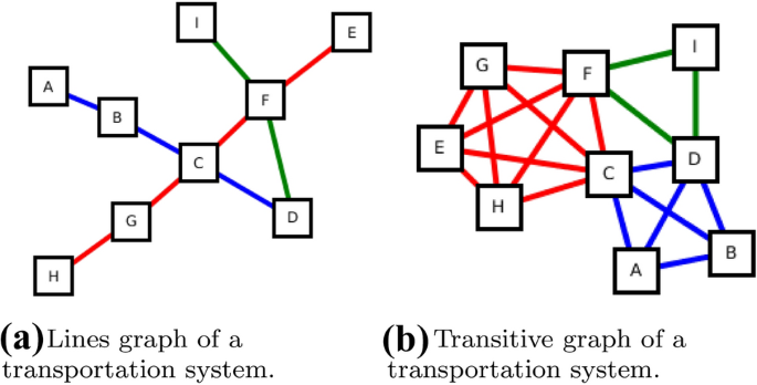

  

  Example for two different representations of the same transportation system

• Wikispeedia West analyzed human navigation paths in information networks. For this project, he collected more than 50,000 trajectories of players playing the game Wikispeedia (West and Leskovec 2012; West et al. 2009). In this game, a player is given (or chooses) a pair of Wikipedia articles and needs to navigate from the one article to the other by following the hyperlinks in the article. The node set of the network is a (sub-)set of Wikipedia articles, and directed edges represent hyperlinks. This network contains 4589 nodes and almost 120,000 edges. We consider only game logs reaching their target article and exclude moves which were revoked by the player via an Undo button. We furthermore exclude solutions longer than 30 steps.

• Wordmorph We use a second dataset containing game logs, from humans playing the game word morph. In this game, a player is given two (English) words of the same length and needs to transform the one word into the other by changing the single letter one by one—where all intermediate words need to be meaningful English words. A valid transformation is for example cry$\rightarrow$dry$\rightarrow$day$\rightarrow$dad$\rightarrow$did. The corresponding network consists thus of nodes representing English words, and there exists an undirected edge between two nodes if the corresponding words have a Hamming distance of 1, i.e., they can transformed into each other by changing one letter. The network consists of 1008 nodes and 8320 (undirected) edges. We use a dataset provided by Kőrösi et al. (2018) who collected human game logs by their publicly available app. We restrict our analysis to 3-letter English words (official English Scrabble words from WordFind)² and only consider solved game logs. This results in approximately 11,000 game logs being used for analysis.

7 Robustness of standard centrality measures

For all datasets, all flow-based centrality variants as well as the corresponding standard centrality measures are computed. The first question which we want to investigate is how robust the standard centrality measures are against deviations of their incorporated process model. If the standard centrality measure and the flow-based measure were very similar to each other, the standard centrality measures would actually be good proxies for the flow-based measures: although the assumptions of the standard centrality measures are not met by the real-world processes, they still would be able to yield sufficiently good results. If, however, the results of the flow-based variants were considerably different from the standard centrality measures, this would imply that the assumptions do have a significant impact on the results. In order to answer this question, we compare the results of standard centrality measures to the results of the flow-based centrality measures.

7.1 Correlation of measures and rankings

We compare the measure values and the corresponding rankings of the flow-based variants to the values and rankings of its corresponding standard centrality value. For the measure values, we computed their Spearman correlation (see Table 5). The measure values can be used for deducing a ranking by assigning each element of V its position number in the node sequence ordered by the measure value: the node with the highest measure value is assigned rank 1 and so forth. There are several strategies for handling ties, i.e., elements of V with equal measure values. In the following, we will use fractional and random ranking. For fractional ranking, nodes with the same measure value are assigned the average rank which they would have gotten without the tie. For random ranking, nodes with equal measure values are assigned distinct rankings where the positioning of these nodes is done randomly. For comparing the resulting rankings, we introduce a metric which we call weighted overlap. The reason why we do not use existing measures, such as Kendall rank correlation (Kendall 1938) or any variant of edit distances (Damerau 1964; Hannak et al. 2013), is their ignorance whether differences in the rankings occur among higher ranked nodes or lower ranked nodes: particularly for centrality indices, a difference in ranking positions among the highest ranked nodes should be penalized more by a metric than a difference among the low-ranked nodes. Furthermore, we are often not interested in the exact ranking position of a node: as long as it is ranked high or low in both rankings, a metric for comparing rankings, should yield a high value. Metrics used for the evaluation of search engine rankings, such as the normalized discounted cumulative gain (Järvelin and Kekäläinen 2002), are also not directly applicable. These are designed to evaluate the quality of a search engine result with respect to the actual relevance of the documents in the resulting ranking. Adapting this measure in order to use it for the comparison of two rankings will yield a non-symmetric evaluation measure which is not desirable. For these reasons, we introduce a metric weighted overlap of rankings $\tau _w$. Based on the idea that the first x elements of both rankings do not need to be in perfect order to get a high value, but should contain nearly the same elements, we consider the overlap of the top x nodes of the two rankings, i.e., the number of elements which are both contained in the top x positions of both rankings. Let $\sigma _1$ and $\sigma _2$ be functions assigning the ranking to each node. We define their overlap of the first x positions as

$$\begin{aligned} ov(\sigma _1,\sigma _2,x) = |\{v\in V|\sigma _1(v)\le x\}\cap \{v\in V| \sigma _2(v)\le x\}|. \end{aligned}$$

Based on this, we first introduce a preliminary measure for comparing two rankings, from which the weighted overlap measure will be derived in the following. The preliminary measure will be referred to as unweighted overlap and is defined as

$$\begin{aligned} \tau (\sigma _1,\sigma _2) = \frac{4}{n^2}\sum _{x=0}^n(x-ov(\sigma _1,\sigma _2,x)). \end{aligned}$$

The idea is the following: for each position in the ranking, i.e., from 1 to n, the overlap of the two rankings up to this position is computed. Two identical rankings would yield an overlap of x for each $x \in \{1,\dots , n\}$; two maximally different rankings, where one is the reverse of the other, would yield an overlap of 0 for x from 1 to $\lfloor n/2\rfloor$, and an overlap of $2x-n$ for the positions x from $\lfloor n/2\rfloor +1$ to n (assumed there are no ties). This can be explained by a simple graphic argument (see Fig. 7): when plotting the overlap of two rankings up to position x as a function of x, the introduced measure $\tau$ considers the area between the overlap curve and the identity line ($x-ov(\sigma _1,\sigma _2,x)$, colored in red). The maximal possible area between the overlap curve and the identity line is, assumed there are no ties, colored grey in the figure. This is due to the fact that from any x to $x+1$, the overlap can increase by at most 2 which implies that the slope of the overlap curve cannot exceed 2. Together with the fact that the overlap of two rankings for $x=n$ is equal to n implies that the maximal possible area between the identity line and any overlap curve is $\frac{n^2}{4}$, depicted as grey area.

Fig. 7

A graphical explanation of the introduced overlap measure $\tau _w$: when plotting the overlap of two rankings $\sigma _1$ and $\sigma _2$ as a function of x, for $x\in [0,n]$, we are interested in the (red) area between the identity line and the overlap function: an area of size 0 implies identical rankings, an area as large as the grey area implies rankings reverse of each other. The example illustrates that the Kendall rank correlation $\tau _K$ is not affected by the position of ranking differences: differences in ranking positions between $\sigma _1$ and $\sigma _2$ have the same effect whether they occur in the top x or bottom x elements. This undesired behaviour is modified by the introduction of a weight which penalizes differences in rankings more when they occur in the top ranked elements (yielding a weighted overlap measure $\tau _w$)

For the preliminary measure $\tau$, the main described problems described for the Kendall rank correlation coefficient are still present: Swaps of ranking positions have the same impact on the value of $\tau$, regardless whether the swap affects high-ranked or low-ranked elements. This is why we introduce a weight function w(x) which weights the difference $x-ov(\sigma _1,\sigma _2,x)$ dependent on x. We chose a weight function $w(x)=n-x$ which is linearly decreasing with x, but also other variants might be applicable.

A further modification is the introduction of a normalization factor $\eta (x)$ for each position x. Introducing $\eta (x)$ is due to the counterintuitive behaviour of the measure that each position x can contribute different values to the sum: Consider the maximal value of each summand $x-ov(\sigma _1,\sigma _2,x)$. For values of $1\le x \le n/2$, each summand $x-ov(\sigma _1,\sigma _2,x)$ can contribute at most x to the sum; for values of $n/2<x\le n$, each summand can contribute at most $n-x$ to the sum. This is why each summand is normalized by its maximal value, realized by a normalization function $\eta (x)$. These modifications lead to the weighted overlap measure:

$$\begin{aligned} \tau _w(\sigma _1,\sigma _2) = \frac{2}{n(n-1)}\sum _{x=1}^{n} w(x)\cdot \frac{x-ov(\sigma _1,\sigma _2,x)}{\eta (x)} \end{aligned}$$

(18)

with

$$\begin{aligned} w(x)=n-x \end{aligned}$$

and

$$\begin{aligned} \eta (x)={\left\{ \begin{array}{ll} x &{} x\le \lfloor n/2\rfloor \\ n-x &{} \text {otherwise} \end{array}\right. } \end{aligned}$$

The factor $\frac{2}{n(n-1)}$ scales the value to the interval [0, 1] where identical rankings yield a value of 0, and reverse rankings yield a value of 1. For other rankings, $\tau _w$ penalizes differences in the rankings more if they occur for higher-ranked nodes than for lower-ranked nodes. Figure 7 shows two examples.

For each flow-based centrality variant and its corresponding standard centrality, we compute the weighted overlap of their rankings, $\tau _w$, and the Spearman correlation coefficient of their values. The results are displayed in Table 5. Note that for $\tau _w$ a value of 0 means a high similarity (equality) of the rankings, while a value 1 means a high dissimilarity of the rankings.

Table 5 Correlation of the process-based centrality measures to their corresponding standard centrality measures and the weighted overlap of the corresponding rankings ($\tau _w$). For the closeness centrality, (if applicable), the process-based in-(/out-)closeness was compared to the standard in-(/out-)closeness

Betweenness measures The Spearman correlation of the standard betweenness centrality to the flow-based variants is positive for all variants and data sets. The correlations of the flow-based betweenness measures to the standard betweenness measures are high, most above 0.7. This suggests that the standard betweenness centrality seems to be quite robust against deviations in its assumed process model in general. Although in all datasets, only a fraction of all node pairs are actually source and target of any observed process trajectory (< 50% for DB1B and London Transport, <1 % for Wikispeedia), it seems that the standard betweenness centrality is robust against a violation of this assumption. For DB1B, it strikes that the correlations as well as the weighted overlap are approximately equal for all measure variants. This could have been expected for the variants $B_R$ and $B_S$ since the observed trajectories are very close to the shortest paths. This is, however, surprising for the variants $B_{SW}$ and $B_{RW}$ incorporating weights since the source-target frequency distribution is skewed: a few node pairs are used very frequently while the majority of node pairs is used rarely or never. When considering the rankings and their weighted overlap, it can be seen that for all other data sets, the rankings from the flow-based betweenness variants incorporating observed trajectories instead of shortest paths, i.e., $B_R$ and $B_{RW}$, differ more from the ranking of the standard betweenness centrality, than the other two flow-based variants, i.e., $B_S$ and $B_{SW}$. Here, we observe values of the weighted overlap up to 0.48. This means that although the observed trajectories do not deviate much from shortest paths, this does have an observable effect on the betweenness measure. The effect is not large—there is still a positive correlation of more than 0.5—but already small deviations from shortest paths do have an impact on the measure value.

Closeness measures For the closeness measures, we find a Spearman correlation of $\ge 0.47$ between the standard closeness centrality and each of the flow-based measures for all datasets. Except for Wikispeedia, the correlations do not show large variations when comparing in- and out-closeness. For the Wikispeedia dataset, the flow-based closeness measures and the standard closeness measure show a correlation of around 0.7 for all in-closeness variants, but seem to be less correlated for all out-closeness variants. When considering the weighted overlap of the rankings for Wikispeedia, the in- and out-variants show a considerable difference to the standard closeness rankings, more than 0.3 for all variants and up to 0.6. For the datasets DB1B and LT (Transitive), the correlations of the flow-based closeness variants to the standard closeness centrality do not vary considerably, they are around 0.88 for all variants for DB1B, and around 0.5 for LT (Transitive).

There is an notable peculiarity concerning the network variants of London Transport for the betweenness and closeness measures: while the correlations of the flow-based variants to the standard centrality is roughly constant (and constantly low) among the variants for the transitive graph, this is different for the lines network: the correlation to the standard centrality is high for the variants considering shortest paths between actually used node pairs, i.e., $B_S$ and $C_S$ and $C_{S'}$, but the correlation drops for the variants which incorporate a weight, i.e., all variants with a subscripted W.

7.2 Ranking deviations

Figures 8 (for betweenness measures) and 9 (for closeness measures) show the ranking position of each node over all measure variants: each point represents a node, its position on the x-axis is the same for all panels and is determined by its ranking position with respect to the standard centrality measure. For each node, its span of ranking positions is computed by computing the difference of its minimal to its maximal ranking position over all measure variants. In Figs. 8 and 9, for each node, its minimal and maximal ranking position over all measure variants is depicted as vertical grey line, thus, the span of ranking positions of a node is the length of the corresponding grey line. Table 6 shows the mean value of the nodes’ spans of ranking positions in absolute ranking positions and relative to the total number of nodes, as well as the range of the nodes’ spans of ranking positions. From Figs. 8 and 9, it can be seen that the rankings of the flow-based centrality measures are clearly positively correlated with its standard centrality measure, for both, betweenness and closeness measures. But there is a considerable deviation of ranks for many nodes when comparing the standard centrality to the flow-based variants. This effect is, however, differently strong for the single datasets for the measure variants. It strikes that the deviation is larger for the game datasets than for the transportation datasets. For Wikispeedia, the mean span of ranking positions is almost 2000 for closeness (out of more than 4000 ranking positions), meaning that on average, the nodes have a variation of ranking positions of almost 2000 positions. The effect is smallest for DB1B, but also there, the average span of ranking positions is around 60 positions which accounts for almost 15% of all ranking positions (see Table 6). Note that a high average value of the nodes’ spans of ranking positions could also be caused by a situation in which only one measure variant produces a ranking which is very different from all others. This is, however, not the case here as it can be seen in Figs. 8 and 9. For DB1B, it strikes that despite a few nodes which are among the top 100 nodes with respect to the standard centrality and drop in importance with respect to at least one flow-based variant, the general ranking deviation is larger for the less highly ranked nodes with respect to the standard centrality. This holds for betweenness and closeness. For both variants of the London Transport system, it strikes that there are several nodes which are not central with respect to the standard centrality measure, but gain in importance with respect to all flow-based variants—except $B_S$.

Fig. 8

Betweenness measures. The ranking positions of the nodes for the standard betweenness and all flow-based betweenness measures. Each point represents one node and its ranking position, and the nodes’ order on the x-axis is determined by its ranking position with respect to the standard betweenness measure. The grey area illustrates the variation of each node’s ranking position over all measure variants

Fig. 9

Closeness measures. Ranking positions of the nodes for the standard in- and out-closeness and all flow-based closeness measures. Each node’s position on the x-axis is determined by its ranking position with respect to standard in-closeness. For each node, its minimal and maximal ranking position with respect to any flow-based variant is depicted by a grey line

Table 6 Spans of ranking positions of the flow-based betweenness and closeness measures: for each node, its span of ranking is computed by subtracting its maximal ranking position with respect to any flow-based variant from its minimal ranking position with respect to any flow-based variant

7.3 Comparison with external variables

Although centrality measures are functions based on the network representation, the ultimate goal is to identify the most important entities of the system represented by the network. Hence, when available, we use properties of the system (and not of the network) which seem to be reasonable proxies for the importance of a system’s entity, for comparison with the ranking results of the flow-based centrality variants. It is clear that in cases when the importance of a system’s entity can directly derived by system’s properties, no proxy methods such as centrality measures on the graph representation are needed. However, in order to evaluate those proxy methods, a comparison with system properties is needed.

In Fig. 10, we show the rankings of the centrality measures and their variants with the corresponding comparison variable: the x-axis shows the ranking position of the nodes where a position on the left corresponds to a high importance ranking position. For each ranking position, the comparison variable of this node is shown by the color at this position.

Fig. 10

Betweenness variants. A comparison of the rankings by the measure variants with external node attributes. The x-axis contains the ranking positions, each node is drawn as a thin vertical line at the corresponding x-position, colored by its external attribute. For DB1B, we color the nodes by the airport categorizations provided by the Federal Aviation Administration (FAA). For Wikispeedia, we compare the nodes’ ranking positions with their number of outgoing links and only show the rankings positions up to 500. For London Transport, the nodes are colored to the station’s zone of the public transport system, where zone 1 contains stations in the inner city center, and zones 2–9 lie concentric around it

DB1B For the air transportation dataset, we use data provided by the Federal Aviation Administration (FAA), part of the United States Department of Transportation. They categorize airports into commercial service airports (publicly owned airports with a scheduled passenger service and at least 2500 passenger boardings each year), cargo service airports (airports served by cargo aircrafts, might also be commercial service airport), reliever airports (airports to relive congestion at Commercial Service Airports, not relevant here), and General Aviation Airports (airports without scheduled passenger service or with less than 2500 passenger boardings each year) (Federal Aviation Administration 2017). Commercial Service airports are further categorized into several sub-types, depending on the annual passenger boardings: non-primary airports (between 2500 and 10000 passengers each year), primary large hubs (more than 1% of all passengers), primary medium hubs (at least 0.25%, but less than 1% of all passenger boardings), primary small hubs (at least 0.05%, but less than 0.25% of all passenger boardings), and primary non-hubs (more than 10,000 passengers yearly, but less than 0.05% of all boardings). Our dataset contains 23 primary large hubs, 27 primary medium hubs, 66 primary small hubs, 228 primary non-hubs, 52 cargo service airports, and 19 general aviation airports. A node representing a city containing more than one airport is then categorized by its largest airport. Figure 10a shows the rankings of the flow-based betweenness variants in comparison with the airport categorization by the FAA which is based on the number of passenger boardings. Since the measure $B_{RW}$ counts in how many passenger journeys of the dataset an airport is contained in, the ranking with respect to $B_{RW}$ and the airport categorizations based on passenger boardings are in great accordance. Airports categorized as large or medium hubs are ranked constantly high over all measure variants. Airports categorized as non-primary airports are ranked constantly low, also for all variants. Only small primary airports (small or no hub) show a stronger variation in their rankings. There is one airport in Saipan located in the Northern Mariana Islands in the Pacific ocean which is low ranked by all variants, but is categorized as small hub by the FAA. The same observation holds for the ranking with respect to $B_{SW}$ since for the passenger journeys, shortest paths and actually taken routes do match in most cases.

Conversely, there is an airport, Orlando Sanford International in Florida, which is categorized as a small hub by FAA, but is ranked high by the measure $B_{R}$ (on position 11 out of 415 nodes). Though, in general, the rankings of the flow-based betweenness measures do show a high segregation of the airport categories, this is not the case for the other datasets.

Wikispeedia For the Wikispeedia dataset, we use a graph-based comparison variable, the article’s number of outgoing links, i.e., its out-degree. This is a good comparison variable in this case since for humans trying to navigate from one article to another, it is a good strategy to first navigate to an article with a high out-degree and then use the large number of possible links to approach the target article.

The categorization of the articles due to their degree was performed such that the categories very small, small, medium and large contain roughly the same number of articles (ca 1k), the category very large only contains almost 100 articles.

We observe that among the top 500 nodes for all betweenness variants, there are mainly articles with very large or large number of outgoing links. Only a few articles with an out-degree smaller than 32 appears in the top 500 nodes of any ranking. The ranking of $B_R$ contains most nodes medium, small and very small degree nodes among the top 500 nodes.

London Transport For London Transport, we use the zones in which the London transport system is divided where zone 1 contains the city center of London and zones 2 to 9 are areas concentric around the city center. Note that the zones do not contain a similar number of stations: while zones 1 and 2 contain more than 60 stations, each, zones 7 to 9 contain 7 stations in total. Figure 10b shows the rankings of the flow-based betweenness measures of the lines network of the London transportation system (results for the transitive variant are not shown, they look similar). For all variants, only stations of zone 1 are among the highest ranked nodes; otherwise, we observe a strong mixing. The highest segregation is found for the ranking of $B_{RW}$—which is intuitive since the stations in the city center are used more frequently.

As a “non-graph based closeness measure,” we use the average travel time for trips starting or ending in a station, also provided by the authority of London Transport (Transport for London 2017). The in-closeness variants are compared to the average travel time of passengers exiting a station and vice versa, see Fig. 11 showing the corresponding plot for the lines variant of the London transportation system. We observe that there is a positive correlation between all measures’ rankings and the corresponding average travel time, and it is though different for the different measures.

Fig. 11

Closeness variants. A comparison of the rankings by the closeness variants with external attributes for London Transport. As a comparison variable, we use the average travel time for passengers entering or exiting a station, provided by Transport for London (2017): in-closeness variants are compared to the average travel time exiting the station (left panel), and ranking of out-closeness variants is compared to the average travel time entering a station (right panel). The average travel time which is a continuous variable is plotted on the y-axis, and each node is represented as a dot at its ranking position

Wordmorph For the dataset containing human navigation paths through a network of words, we use a word frequency list of English words based on the Corpus of Contemporary American English which contains the frequency of each word in the text corpus, provided by Davis (2008). They provide a score (called frequency rank in the following) for each word which is a function of its frequency of occurrence in the text corpus and its dispersion (Juilland and Chang-Rodriguez 1964), a measure for quantifying how evenly a word is distributed among the parts of the text corpus. We use the frequency rank as a comparison variable to the ranking position by the flow-based centrality measures, where a low value of frequency rank implies a high frequency and a high dispersion. For words contained in the network which are inflected forms, such as are is an inflected form of the verb be, the score of its base form, here be, is used. For words which are contained several times in the word frequency list, such as use as noun and as verb, the one with the higher score is kept. Figure 10d shows that especially for $B_R$ (and also for $B_{RW}$), nodes with a higher frequency of rank occur more often among the highly ranked nodes than for the standard betweenness centrality. A possible reason could be—which is only a speculation at this point—that the players tend to navigate over words which are more familiar to them rather than over words which are not in their daily vocabulary.

8 Effect on high-ranked nodes

In most situations when applying centrality measures on a network, we are interested in the most central nodes which is why the results of a centrality measure should be especially reliable for the highly ranked nodes. If a centrality is able to identify the most important nodes, evaluated by a suited criterion, the exact ranking positions on the lower ranking positions are less relevant. When considering the complete ranking induced by a centrality measure, as done in the previous section, this aspect is not regarded. We hence restrict the following analysis on those nodes which are among the 10 most central nodes with respect to any of our introduced measure variants.

Figures 12 (for betweenness) and 15 (for closeness) show the ranking behavior of those nodes which are among the 10 most central nodes with respect to any standard or flow-based measure, separately for betweenness and closeness: for each of those nodes, its ranking position with respect to all variants is shown.

Fig. 12

Top 10 nodes (betweenness) Ranking positions with respect to all betweenness centrality variants of those nodes which are among the 10 most central nodes with respect to at least one centrality variant. Top nodes have rank 1 (top of each plot), the order of the line colors is due to the node’s standard betweenness centrality

8.1 Betweenness measures

We find that for none of the datasets, the 10 highest ranked nodes are the same for all variants, and there are actually a lot of ranking position changes among those nodes.

DB1B For DB1B, we find that all considered nodes are at least among the top 60 of all measures, most even among top 30 of all measures. All measure betweenness variants identify large airports as most central. There is one node, representing the airport Anchorage in Alaska which is ranked as second most central node by the standard betweenness centrality, but drops in importance with respect to all flow-based betweenness measures. When looking at the structure of the airport network, the reason for this effect can be seen. Anchorage serves as gateway between airports in the contiguous United States, i.e, the adjoined US states, to several small airports in Alaska in some sense. It is not true that any airport in Alaska can only be reached via Anchorage—there are also direct flight connections from airports in contiguous US to Alaska, but the network consists of a densely connected 46-core: a subgraph consisting of 56 nodes in which each node has a degree of at least 46. This 46-core almost forms a clique and hence all nodes within have a distance of 1 to each other and a high betweenness value. All airports of this core are, however, located in the contiguous United States, no Alaskan airport is part of this core—and Anchorage is well connected to nodes in this core and to all Alaskan airports. Figure 13 shows the corresponding extract of the network: all airports in Alaska and their direct neighbors. The node colors indicate to which k-core the node belongs to. Red nodes are part of the large densely connected core. Anchorage is directly connected to 24 nodes within the core and more than half of all Alaskan airports can only reached via Anchorage. This is why the node Anchorage gets a high standard betweenness value. When, however, the observed passenger journeys are incorporated into the betweenness value, this high centrality value vanishes because only a small fraction of all passenger journeys involve Anchorage or any other Alaskan airport. This is especially the case when the flow-based betweenness centrality incorporates weights. Still, also for those variants, the node Anchorage is still among the 60 most central nodes.

Fig. 13

An extract of the DB1B air transportation network: All Alaskan airports and their direct neighbors. The color shows to which k-core the nodes belong in the complete network: Red nodes belong to the largest core and most densely connected core of the network. Nodes representing Alaskan airports are labeled as AK, nodes representing airports in the contiguous United States are labeled as US

Wikispeedia For Wikispeedia, we can make several observations: first, the set of nodes which are among the top 10 nodes for any variant is larger than for DB1B and the differences of the rankings is also larger: there are nodes which are not even among the top 1000 nodes with respect to some variants, but reach the top 10 with respect to another measure. At the same time, for all five measure variants, the 5 most central nodes are rather stable in their ranking. The node of the article United States is the most central node for all measure variants. This reflects a popular strategy for playing Wikispeedia: using the article of United States as a landmark—first navigate to United States article, then from there to the target article). Furthermore, there are four nodes, namely the articles Brain, Viking, Asteroid, and Telephone which are boosted into the top 10 nodes for $B_{SW}$ and $B_{RW}$, i.e., the weighted versions. This is actually due to the data collection method. West and Leskovec (2012) describe that there were four article pairs which were suggested to the players as source and target more often. This is why the node pairs (Asteroid,Viking) and (Brain,Telephone) have the highest frequency and the corresponding nodes gain in importance when incorporating the source-target-frequency. The four other nodes of the promoted source-target pairs show the same effect, but less strong such that they do not reach the top 10 nodes of any measure.

London Transport For London Transport datasets, we find different results for the two versions of the network. While for the transitive network version of the London transportation system, London’s main station King’s Cross St. Pancras is ranked highest by all betweenness variants, this is not the case for the line graph version. Here, the node representing King’s Cross St. Pancras is only the most central node for the flow-based variants incorporating real trajectories, i.e., $B_R$ and $B_{RW}$. For the lines version, it is the node representing the station Baker Street which is most central with respect to the standard betweenness centrality, but not with respect to any of the flow-based betweenness variants. Both stations, King’s Cross St. Pancras and Baker Street, serve as junction point for the Underground network, they both serve a high number of different underground lines, namely six and five, respectively. Therefore, and due to the structure of the lines network—a more densely connected core with chain-like structures appended to it—these two nodes are contained in many shortest paths between node pairs. Because of its position in the lines network, the node Baker Street is contained in more shortest paths when considering all node pairs than the node King’s Cross St. Pancras³ which is why it is higher ranked by the standard betweenness centrality. The top ranking position of the node Baker Street is lost when taking into account the real usage of the system, especially when considering the actual amount of passenger flow between the stations. Then, King’s Cross St. Pancras gains in importance.

An interesting effect caused by the modeling of the system can be observed here. For the lines graph of the London transportation system, the nodes Holborn and London Bridge, both with a standard betweenness ranking position lower than 100, get both a top 10 ranking position with respect to the flow-based betweenness variants $B_R$ and $B_{RW}$. However, with respect to the variants $B_S$ and $B_{SW}$, they do not reach the high ranking positions. It turns out that this is an effect of the modeling of the system: the system is modeled as one network where an edge represents an underground connection between two stations; this can, however, be served by different underground lines. The edges are weighted by travel time, though, additional time necessary for changing a line (get off the line, change the platform, possibly waiting for the next line, enter the line) are not modeled, still. Therefore, an algorithm computing a shortest path in this graph will—although considering the edge weights—may yield paths that might not be the fastest (or most convenient) in reality. The ranking behavior of the node Holborn is a consequence of this effect: especially in the city center where many stations are served by more than one line and the stations are close to each other in means of travel time, the shortest path in the graph representation is not the realistically taken journey. Figure 14 shows a very small extract of the network where the edge colors indicate which underground line serves this connection, the corresponding travel times are also shown. It shows the reason why the node Holborn gains in importance when real journeys are used for the measure computation: in the most cases, passengers will only change lines if this choice is—time for changing included—substantially faster. A betweenness measure using shortest paths on this graph representation, however, will yield paths with several line changes. Passengers traveling from King’s Cross Pancras to South Kensington for example will mostly take the Piccadilly line which takes 13 min. But the shortest path in this graph is from King’s Cross St. Pancras to Green park by the Victoria line and then to Knightsbridge by the Piccadilly line length of which is 9 min in total. Depending on the weights of the edges, it can become worse: in the extreme case, the shortest path algorithm may return a path in which no consecutive two edges are of the same line. This effect occurs often with the real passenger journeys of the dataset and the described modeling of the system, particularly often concerning the node Holborn. This explains the finding that the node Holborn is not central with respect to any measure counting shortest paths in the graph, but is central with respect to any measure counting real trajectories it is contained in.

Fig. 14

A small extract of the lines graph for the London transportation system. The edge labels indicate the travel time between the stations which are taken as edge weights, and the edge colors indicate which underground lines serve the corresponding connection

The same effect occurs for the transitive graph of the London transportation system because also here, changes of the line are not penalized in the algorithm computing the shortest paths. For the transitive graph, however, it can also have the opposite effect than before: nodes can lose importance when taking into account real passenger journeys instead of shortest paths, as it is the case for the station Moorgate. Moorgate is among the top 10 nodes with respect to the variants counting shortest paths, i.e., standard betweenness, $B_S$, and $B_{SW}$, but is only ranked on position 31 and 29 for the variants $B_R$ and $B_{RW}$, respectively. For passengers, <>there is often no need to change train at Moorgate which is why their journey (in the transitive graph representation) does not contain this node. In the graph representation, though, there is a shorter path when using the node Moorgate. This is why it is contained in the shortest paths and is highly ranked by measures counting shortest paths.

Wordmorph For the Wordmorph dataset (see Fig. 12e), we find a high accordance among the rankings of the standard betweenness centrality, and the flow-based variants $B_S$ and $B_{SW}$, as well as among the rankings of $B_R$ and $B_{RW}$. The accordance between those measures can be explained by the source-target distribution of the game logs: by far the most source-target pairs are used by exactly one player (more than 10,000 pairs) while only a few (less than 100) are used by two or three players. This explains why the rankings of the flow-based betweenness variants incorporating weights does not differ considerably from the corresponding flow-based variants without weights. When changing from counting shortest paths to counting real trajectories, i.e., from the variants $B_{S\cdot }$ to $B_{R\cdot }$, we observe considerable changes in ranking positions: the nodes ART and ARE increase their ranking position 111 to 2 and 54 to 3, respectively. On the same time, the nodes OES, AYE and SOY drop in importance when real paths are considered. Interestingly, the node AIT is among the 3 most central nodes with respect to all measure variants. Gulyás et al. (2020) analyze the navigation paths of this dataset in detail and find that each player builds her own scaffold of the network which she uses in the following for finding short, but not optimal navigation paths. They find that the overlap of the individual scaffolds is very low, hence each player builds her own individual scaffold for effective navigation. Still, incorporating the navigation paths into the betweenness centrality does show a considerable effect on the node ranking.

8.2 Closeness measures

Figure 15 shows the ranking behaviors of the closeness variants. The plots contain those nodes which are among the top 10 with respect to any of the closeness variants, this is done separately for the in- and out-variants. We only show the results for the out-closeness variants, the in-closeness variants show similar effects.

Fig. 15

Top 10 nodes (closeness). Ranking positions with respect to all centrality variants of those nodes which are among the 10 most central nodes with respect to at least one centrality variant. Top nodes have rank 1 (top of each plot), the order of the line colors is due to the node’s standard closeness centrality

DB1B For the air transportation network (see Fig. 15a), we see that there is very limited variation of changes in ranking positions among the considered nodes. Particularly the rankings of the standard closeness and the variants $C_S, C_{S'}$, and $C_R$, i.e., those variants which do not incorporate any weights, show a high similarity. This is not surprising since the actual observed trajectories are shortest paths in the most cases. The node rankings of the variants $C_{SW}$ and $C_{RW'}$ exhibit a noticeable behavior: a small set of nodes, i.e., the nodes representing the airports Denver, Minneapolis/St.Paul, Houston, and Phoenix, which are most central with respect to the other variants, drop in importance while other nodes such as Miami increase their ranking position by almost 20 positions. This is due to the amount of passenger traffic between the airports: Among all airport pairs, the pair (Miami, New York) has the second highest number of passenger traffic between them (behind (San Francisco, Los Angeles)). On the same time, all nodes shown in Fig. 15a are part of 46-core of the network including all major US airports. All nodes contained in this 46-core have a distance 1 to each other, and a distance of 2 to most of the remaining nodes. No node contained in the 46-core has a distance larger than 3 to any other node, and particularly those nodes shown in the figure have a distance of larger of 2 to only very few nodes (in most cases, to exactly one node, and, for the case of Miami, to 5 other nodes). Hence, when incorporating the actual passenger traffic between the airports such that the distance between airports with a high passenger flow has a larger impact on the measure value than the distance between airports with a smaller passenger flow, this makes a difference: the highly demanded node pair (Miami, New York) with a distance of 1 boosts the closeness ranking of both, Miami and New York. When considering solely the network structure, Denver has a smaller average distance to the remaining nodes, and Denver even has a higher total passenger traffic than Miami. Anyhow, when weighting the distances by the corresponding passenger traffic, the nodes Miami and New York are ranked higher than Denver.

Wikispeedia For Wikispeedia, the effect on the nodes’ ranking of incorporating the actually observed trajectories into the closeness measure is much larger than for the other datasets. The effect is also clearly visible when only considering those nodes which are among the top 10 most central ones with respect to any variant. There are nodes in- or decreasing their ranking position by more than 1000 positions. Interestingly, for Wikispeedia, there exists also two measure variants for which several nodes seem to switch their ranking positions, namely $C_R$ and $C_{RW}$. This is however not the same variant for which this effect occurred for DB1B. Regarding the measure variants for which DB1B showed this behavior, the ranking behavior of Wikispeedia is rather stable. For $C_S$ and $C_{RW}$, though, a few nodes’ centrality value increases considerably compared to the remaining measure variants. For $C_{RW}$, i.e., a measure variant taking into account real observed trajectories and their frequency of occurrence, we find–as for the betweenness variants–an impact of the data collection method. The source of those four node pair which were suggested to the players with an increased frequency, can be found ranked highly with respect to $C_{RW}$: Brain, Asteroid, Theatre and Pyramid are all among top 8 nodes. Furthermore, when considering the node pairs used most often by the players, it seems that the article Batman was a popular start article. This is reflected in the ranking of $C_{RW}$, it is ranked as second node. Regarding the ranking with respect to $C_{S}$, we observe that for the in- and out-version of $C_S$ the articles of Adolf Hitler and Jesus to be among the three highest ranked nodes. This seems to be due to the game variants 5-clicks-to-Jesus and Clicks to Hitler which are believed to be the original forms of the game where the player needs to navigate from a randomly chosen Wikipedia article to the article of Jesus or Adolf Hitler, respectively. We speculate that due to the prominence of those two game versions, players of Wikispeedia often chose those articles as source and especially as target. This would explain the rise in ranking of these articles for $C_S$. A further interesting effect concerns the articles Driving on the left or right, List of countries, and List of circulating currencies. These articles all include links to the articles of all countries which leads to a high ranking position for the standard out-closeness centrality. However, since these articles were not used at all (Driving on the left or right) or only a few times by the players for navigating through the network, their ranking position drops massively for the flow-based closeness variants.

London Transport For the two network versions of the London Transport system, we find—as for the betweenness measures—that the nodes’ ranking behaviour for the closeness variants differs considerably between the lines graph and the transitive graph. As before for the betweenness centrality, the rankings of the top 10 nodes of the flow-based closeness variants are rather stable for the transitive graph, while there are large changes in ranking positions for the lines graph. But while the standard betweenness centrality and the flow-based betweenness variants showed a similar ranking behaviour, this is not the case for the closeness variants (see Fig. 15d): Most nodes ranked high by the standard closeness drop in importance when measured by the flow-based variants–and vice versa.

Wordmorph For the closeness measure variants, the game datasets, Wikispeedia and Wordmorph show similar effects: for both datasets, the variation of rankings is quite large: their average span of ranking positions (see Table 6) is 44% of all ranking positions. Among the nodes which are among the 10 most central nodes with respect to at least one measure variant, we find nodes with a span of ranking positions of more than 700 positions: the node ARE for example increases its ranking position from 813 (standard closeness) to 3 and 4 for several flow-based measures. Interestingly, for both game datasets, the rankings of $C_R, C_{RW'}, C_S'$, and $C_{SW}$ are quite stable for these selected nodes, while the measures $C_S$ and $C_{RW}$ yield totally different central nodes. All flow-based variants, however, yield different central nodes than standard closeness centrality.

9 Conclusion

Centrality measures such as closeness and betweenness centrality contain an implicit process model: they assume the presence of something flowing through the network and make assumptions of how it is flowing through the network. It is clear that a centrality measure can only measure the importance of the nodes with respect to a process with those properties. For example, classic closeness and betweenness centrality both assume the process moving on shortest paths. Furthermore, an equal frequency of communication between all node pairs is assumed since for both measures, the relevant quality, fraction of the number of shortest paths in the case of betweenness and distance in the case of closeness, is equally aggregated for all node pairs. That those assumptions are not true for most real-world processes is not new. For this reason, other centrality measures have been introduced which use different process model, for example random walk betweenness or flow betweenness. In this work, we aimed at answering the following question: how much does it matter in reality that those assumptions are not met? In order to answer this question, we collected four datasets of real-world transfer processes and replaced the simple process model of the centrality measures by the behaviour of the real-world process. We introduced several variants of flow-based closeness and betweenness centrality measures which partly use the simple process model and partly the real-world process. For example, one flow-based betweenness variant keeps the assumption of shortest paths and counts those, but only between node pairs which were actually source and target of the real-world process.

For the betweenness centrality, we find a high correlation of the standard betweenness centrality to all flow-based variants indicating that for the used datasets, the betweenness centrality seems to quite robust against deviations from its process model. On the same time, we find a considerable number of nodes in all datasets whose ranking position changes substantially. For the closeness centrality, the correlation of the flow-based variants to the standard closeness is generally lower than for betweenness. Also here, in all datasets, we find nodes with large ranking variations.

Comparing the datasets, we find that there is a larger variation of rankings for the two datasets containing game logs than for the two datasets containing passenger journeys. This might be due to the fact that for passenger journeys, the assumption of shortest paths is a better approximation than for human navigation paths in games. Nevertheless, also for those datasets, the changes in rankings are remarkable.

When examining the resulting rankings in detail, we are able to detect several anomalies of the datasets or the standard measures. As an example, standard betweenness centrality assigns a high value to the node representing the airport Anchorage in the US airport network. This is due to its position in the network being on all almost shortest paths between airports in the contiguous states and Alaska. When incorporating the actual passenger journeys into the measure, the centrality value of the node Anchorage decreases because most airline traffic takes place within the densely connected airports in the contiguous states and only a small fraction of passenger journeys involve any Alaskan airport.

Whether this effect is desired or not depends on the application scenario. The presence of this effect, however, shows that a violation of the assumptions contained in the centrality measures does have an impact on the measure results. This is relevant for the applicability of centrality measures: when applying a centrality measure on a network, we are interested in identifying the most important nodes with respect to a certain process. If the corresponding process violates the measure’s assumptions, the results need to be interpreted with care.

References

Anthonisse JM (1971) The rush in a directed graph. Stichting Mathematisch Centrum Mathematische Besliskunde (BN 9/71):1–10
Bavelas A (1948) A mathematical model for group structures. Hum Organ 7(3):16–30
Bockholt M, Zweig KA (2018) Process-driven betweenness centrality measures. In: Lecture notes in social networks. Springer, Cham, pp 17–33. https://doi.org/10.1007/978-3-319-90312-5_2
Bockholt M, Zweig KA (2019) Why we need a process-driven network analysis. In: Complex networks and their applications VIII. Springer, Cham, pp 81–93. https://doi.org/10.1007/978-3-030-36683-4_7
Bonacich P (1972) Factoring and weighting approaches to status scores and clique identification. J Math Sociol 2(1):113–120
Bonacich P (1987) Power and centrality: a family of measures. Am J Sociol 92(5):1170–1182
Borgatti SP (2005) Centrality and network flow. Soc Netw 27(1):55–71. https://doi.org/10.1016/j.socnet.2004.11.008
Borgatti SP, Everett MG (2006) A graph-theoretic perspective on centrality. Soc Netw 28(4):466–484. https://doi.org/10.1016/j.socnet.2005.11.005
Csoma A, Kőrösi A, Rétvári G, Heszberger Z, Bíró J, Slíz M, Avena-Koenigsberger A, Griffa A, Hagmann P, Gulyás A (2017) Routes obey hierarchy in complex networks. Sci Rep. https://doi.org/10.1038/s41598-017-07412-4
Damerau FJ (1964) A technique for computer detection and correction of spelling errors. Commun ACM 7(3):171–176. https://doi.org/10.1145/363958.363994
Davis M (2008) The corpus of contemporary American English (Coca): 600 million words, 1990-present. https://www.english-corpora.org/coca/
Dodds PS (2003) An experimental study of search in global social networks. Science 301(5634):827–829. https://doi.org/10.1126/science.1081058
Dolev S, Elovici Y, Puzis R (2010) Routing betweenness centrality. J ACM 57(4):1–27. https://doi.org/10.1145/1734213.1734219
Dorn I, Lindenblatt A, Zweig KA (2012) The trilemma of network analysis. In: Proceedings of the international conference on advances in social networks analysis and mining (ASONAM), Washington, DC, USA, pp 9–14. https://doi.org/10.1109/ASONAM.2012.12
Federal Aviation Administration (2017) National Plan of Integrated Airport Systems (NPIAS) 2017–2012, report of the secretary of transportation to the united states congress edn. U.S. Department of Transportation. http://www.faa.gov/airports/planning_capacity/npias/reports/
Freeman LC (1977) A set of measures of centrality based on betweenness. Sociometry 6:35–41
Freeman LC (1978) Centrality in social networks conceptual clarification. Soc Netw 1(3):215–239
Freeman LC, Borgatti SP, White DR (1991) Centrality in valued graphs: a measure of betweenness based on network flow. Soc Netw 13(2):141–154
Friedkin NE (1983) Horizons of observability and limits of informal control in organizations. Soc Forces 62(1):54–77. https://doi.org/10.1093/sf/62.1.54
Gao L, Wang F (2002) The extent of AS path inflation by routing policies. In: Global telecommunications conference, 2002 (GLOBECOM’02). IEEE. https://doi.org/10.1109/glocom.2002.1189018
Ghosh R, Lerman K (2012) Rethinking centrality: the role of dynamical processes in social network analysis. CoRR http://arxiv.org/abs/1209.4616
Gulyás A, Bíró J, Rétvári G, Novák M, Kőrösi A, Slíz M, Heszberger Z (2020) The role of detours in individual human navigation patterns of complex networks. Sci Rep. https://doi.org/10.1038/s41598-020-57856-4
Hannak A, Sapiezynski P, Kakhki AM, Krishnamurthy B, Lazer D, Mislove A, Wilson C (2013) Measuring personalization of web search. In: Proceedings of the 22nd international conference on World Wide Web—WWW’13. ACM Press, London. https://doi.org/10.1145/2488388.2488435
Järvelin K, Kekäläinen J (2002) Cumulated gain-based evaluation of IR techniques. ACM Trans Inf Syst 20(4):422–446. https://doi.org/10.1145/582415.582418
Juilland A, Chang-Rodriguez E (1964) Frequency dictionary of Spanish words. Mouton de Gruyter, The Hague
Katz L (1953) A new status index derived from sociometric analysis. Psychometrika 18(1):39–43
Kendall MG (1938) A new measure of rank correlation. Biometrika 30(1–2):81–93. https://doi.org/10.1093/biomet/30.1-2.81
Kőrösi A, Csoma A, Rétvári G, Heszberger Z, Bíró J, Tapolcai J, Pelle I, Klajbár D, Novák M, Halasi V, Gulyás A (2018) A dataset on human navigation strategies in foreign networked systems. Sci Data. https://doi.org/10.1038/sdata.2018.37
Koschützki D, Lehmann KA, Peeters L, Richter S, Tenfelde-Podehl D, Zlotowski O (2005) Centrality indices. In: Brandes U, Erlebach T (eds) Network analysis: methodological foundations, lecture notes in computer science, vol 3418. Springer Berlin, pp 16–61. https://doi.org/10.1007/978-3-540-31955-9_3
Manley E, Addison J, Cheng T (2015) Shortest path or anchor-based route choice: a large-scale empirical analysis of minicab routing in London. J Transp Geogr 43:123–139. https://doi.org/10.1016/j.jtrangeo.2015.01.006
Meiss MR, Menczer F, Fortunato S, Flammini A, Vespignani A (2008) Ranking web sites with real user traffic. In: Proceedings of the international conference on Web search and web data mining—(WSDM’08). ACM Press, London. https://doi.org/10.1145/1341531.1341543
Milgram S (1967) The small world problem. Psychol Today 2(1):60–67
Newman ME (2005) A measure of betweenness centrality based on random walks. Soc Netw 27(1):39–54
Nieminen J (1974) On the centrality in a graph. Scand J Psychol 15(1):332–336. https://doi.org/10.1111/j.1467-9450.1974.tb00598.x
Noh JD, Rieger H (2004) Random walks on complex networks. Phys Rev Lett. https://doi.org/10.1103/physrevlett.92.118701
Page L, Brin S, Motwani R, Winograd T (1999) The pagerank citation ranking: Bringing order to the web. Tech. rep, Stanford InfoLab
RITA TransStat (2016) Origin and Destination Survey database (DB1B). https://www.transtats.bts.gov/DatabaseInfo.asp?DB_ID=125
Rosvall M, Esquivel AV, Lancichinetti A, West JD, Lambiotte R (2014) Memory in network flows and its effects on spreading dynamics and community detection. Nat Commun. https://doi.org/10.1038/ncomms5630
Sabidussi G (1966) The centrality index of a graph. Psychometrika 31(4):581–603
Schoch D, Brandes U (2016) Re-conceptualizing centrality in social networks. Eur J Appl Math 27(6):971–985. https://doi.org/10.1017/s0956792516000401
Scholtes I, Wider N, Garas A (2016) Higher-order aggregate networks in the analysis of temporal networks: path structures and centralities. Eur Phys J B 89(3):1–15
Stephenson K, Zelen M (1989) Rethinking centrality: methods and examples. Soc Netw 11(1):1–37
Sudarshan Iyengar S, Veni Madhavan C, Zweig KA, Natarajan A (2012) Understanding human navigation using network analysis. Top Cognit Sci 4(1):121–134
Transport for London (2017) Rolling Origin and Destination Survey (RODS). http://www.tfl.gov.uk/info-for/open-data-users/our-feeds
Weng L, Ratkiewicz J, Perra N, Gonçalves B, Castillo C, Bonchi F, Schifanella R, Menczer F, Flammini A (2013) The role of information diffusion in the evolution of social networks. In: Proceedings of the 19th ACM SIGKDD international conference on knowledge discovery and data mining (KDD’13). ACM, New York, pp 356–364. https://doi.org/10.1145/2487575.2487607
West R, Leskovec J (2012) Human wayfinding in information networks. In: Proceedings of the 21st international conference on World Wide Web. ACM, pp 619–628
West R, Pineau J, Precup D (2009) Wikispeedia: an online game for inferring semantic distances between concepts. In: IJCAI international joint conference on artificial intelligence, pp 1598–1603
Yuan J, Zheng Y, Zhang C, Xie W, Xie X, Sun G, Huang Y (2010) T-drive: driving directions based on taxi trajectories. In: Proceedings of the 18th SIGSPATIAL international conference on advances in geographic information systems. ACM, pp 99–108
Zheng Y, Zhang L, Xie X, Ma WY (2009) Mining interesting locations and travel sequences from GPS trajectories. In: Proceedings of the 18th international conference on World wide web. ACM, pp 791–800
Zhu S, Levinson D (2015) Do people use the shortest path? An empirical test of wardrop’s first principle. PLoS ONE 10(8):e0134322. https://doi.org/10.1371/journal.pone.0134322
Zweig KA (2016) Network analysis literacy. Springer, Vienna. https://doi.org/10.1007/978-3-7091-0741-6
Funding
Open Access funding enabled and organized by Projekt DEAL.
Author information
Authors and Affiliations
Corresponding author
Ethics declarations
Conflict of interest
The authors declare that they have no competing interests.
Code availability
The source code used for analysis during the current study is available from the corresponding author on reasonable request.
Additional information
Publisher's Note
Springer Nature remains neutral with regard to jurisdictional claims in published maps and institutional affiliations.
Rights and permissions
Open Access This article is licensed under a Creative Commons Attribution 4.0 International License, which permits use, sharing, adaptation, distribution and reproduction in any medium or format, as long as you give appropriate credit to the original author(s) and the source, provide a link to the Creative Commons licence, and indicate if changes were made. The images or other third party material in this article are included in the article's Creative Commons licence, unless indicated otherwise in a credit line to the material. If material is not included in the article's Creative Commons licence and your intended use is not permitted by statutory regulation or exceeds the permitted use, you will need to obtain permission directly from the copyright holder. To view a copy of this licence, visit http://creativecommons.org/licenses/by/4.0/.
About this article
Cite this article
Bockholt, M., Zweig, K.A. A systematic evaluation of assumptions in centrality measures by empirical flow data. Soc. Netw. Anal. Min. 11, 25 (2021). https://doi.org/10.1007/s13278-021-00725-3
Received:
Revised:
Accepted:
Published:
DOI: https://doi.org/10.1007/s13278-021-00725-3