
Abstract
The shale gas experiences many different spatial scales during its flow in the reservoir, which will engender different flow mechanisms. In order to accurately simulate the production performance of shale gas well, it is essential to establish a multi-continuum model for shale gas reservoir. Based on the geometrical scenario of multistage horizontal well fracturing, this paper builds up a triple-continuum model incorporating three systems: matrix with extremely low permeability, less permeable natural fractures and highly permeable hydraulic fractures. This numerical model employs Langmuir adsorption equation to present the influence of desorption gas in matrix and considers the Klinkenberg effect in matrix and natural fractures by adjusting the apparent permeability. The solution of this model is achieved using implicit scheme. Eventually, this model is applied on the single well production situation in a synthetic reservoir, production decline curves and cumulative production curves are obtained, then the sensitivity analysis is made on various kinds of parameters; thus, the influences of these parameters on production rate are obtained: The gas rate will rise with the increase in hydraulic fracture half-length, meshing size, Langmuir volume and Langmuir pressure, but with the decrease in hydraulic fracture spacing.
Introduction
Nowadays, shale gas production has been making a significant contribution to the world’s gross energy supply (Li 2009) and accounts for over 50 % of American natural gas production (Montgomery et al. 2005). The exploration shows that China is also abundant in terms of the total recoverable shale gas reserves (Hu et al. 2010). Shale gas reservoir distinguishes itself by its extremely low permeability and low porosity, which engenders great difficulty on the exploitation and production of shale gas (Curtis 2002; Li et al. 2015). In addition, the pore size in shale matrix is only about 2–50 nm and 0.1–5 μm for the natural fractures (Sondergeld et al. 2010). Instead of the conventional method, the effective and economic development of shale gas reservoir requires the formation to be hydraulically fractured, and the multistage hydraulic fracturing method has been prevalently employed in shale gas reservoir (Ozcan et al. 2014).
Naturally fractured reservoir (NFR) can be defined as a reservoir contains a connected network of fractures created by natural processes and proved to have an effect on fluid flow (Javadpour 2009; Sun et al. 2016). NFR contains more than 20 % of the world’s hydrocarbon reserves (Sarma and Aziz 2006). Shale gas reservoir generally contains natural fractures; thus, shale gas reservoir can be classified into NFR. In shales, natural fractures provide permeability and the matrix provides storage for most of the gas (Bello and Wattenbarger 2010). The gas molecules are stored by a combination of compression in the pores and adsorption on the surface of the solid shale matter (Bello and Wattenbarger 2008). It is believed that compared to the induced fractures, the permeability of natural fractures is too small to be considered. Yet this is proved to be wrong because the natural fracture network can actually enhance the productivity of the reservoir greatly (Cipolla et al. 2010); thus, the local natural fractures shall not be ignored.
From the nanoscale matrix to the hydraulic fractures whose width is several millimeters, shale gas experiences many different spatial scales during its flow in the reservoir (Sheng et al. 2012; Guo et al. 2015). According to different spatial scales, the flow of gas in the shale formation will result in many different mechanisms (Jiang and Wang 2014; Xu et al. 2015). As the natural fractures and the hydraulic fractures present a big difference in terms of fracture conductivity and connectivity, it is more realistic to assume fractures having different properties (Hassan and Wattenbarger 2011).
Commonly, the dual-porosity model is often used for the simulation of oil and gas reservoir, but only two continuums are unable to fully describe the multi-mechanism and multi-scale gas flow in shale formation (Cheng and Dong 2012). In order to accurately simulate the complicated shale gas flow and production, multi-continuum models shall be built up (Zhu and Zhang 2013). Furthermore, some microscopic mechanisms, such as desorption and diffusion effect, should be considered in the model as well (Ozkan et al. 2010); thus, triple-continuum model begins to emerge (Fig. 1).

Illustration of gas flow from nanoscale to macroscale
The first triple porosity was introduced by Abdassah and Ershaghi (1986), and they divided the matrix to have different properties with single fracture. Then Al-Ahmadi and Ershaghi (1996) first assume the fractures to have different properties, their model was presented using a radial system, and the natural fractures and the hydraulic fractures can both feed the well. Drier (2004) improved the triple-continuum model originally proposed by Al-Ahmadi and Ershaghi (1996) by considering transient flow condition between natural fractures and hydraulic fractures. Bello and Wattenberger (2008, 2009, 2010) applied the triple-continuum model to analyze the production rate in horizontal well in tight fractured reservoirs. Ozkan et al. (2009) proposed a trilinear model comprising three continuous media: finite conductivity hydraulic fractures, dual-porosity inner reservoir between the hydraulic fractures and outer reservoir beyond the tip of the hydraulic fractures. Apaydin et al. (2012) examine the effects of matrix micro-fractures on effective matrix permeability of a dual-porosity medium. They stated that matrix micro-fractures accelerate production by providing earlier and more effective contribution of the matrix into flow rates. Therefore, the multi-continuum model for shale gas reservoir commonly comprises three media: matrix, natural fractures and hydraulic fractures, which is also called dual-fracture model (Al-Ahmadi and Ershaghi 1996).
The triple-continuum model has undergone great development recently, and models for reservoirs with sophisticated geometries and conditions have been built up in previous work. The findings show that the triple-continuum model can capture the reservoir heterogeneity very well (Al-Ahmadi 2010). Nonetheless, most previous triple-continuum models were solved using analytical method instead of numerical approach to predict the transient pressure in the reservoir. In addition, diffusion mechanism, which is proved to have significant impact on gas flow, was rarely considered in previous models. In this work, a new numerical triple-continuum model incorporating desorption and diffusion is proposed and applied for the production simulation in fractured shale gas reservoir.
Incorporated mechanisms
Adsorption and desorption of shale gas
Shale gas can exist as free gas phase or as adsorbed gas on solids in pores, and the methane molecules are mainly adsorbed to the carbon-rich components, i.e., kerogen (Lu et al. 1995). As observed, the adsorbed gas accounts for a significant fraction of gas reserves in place. With the drawdown of the formation pressure, the adsorbed gas is released from the surface of solids and becomes free gas, contributing to the total production. In this work, the mass flux of the adsorbed gas in a micro-unit within a short time is described as:
Here the Langmuir adsorption model is employed to represent the adsorbed gas content V E:
Where V L stands for the Langmuir volume, p L is the Langmuir pressure, and p is the reservoir pressure.
Klinkenberg effect
In low-permeability shale gas reservoirs with small pore space, the Klinkenberg effect may alter the permeability significantly, especially in low reservoir pressure conditions (Wu et al. 1998). In this work, Klinkenberg effect is incorporated into the gas flow equations by modifying the apparent permeability of gas as a function of pressure (Wu et al. 2009):
where k a is the apparent permeability of the gas phase; k i is the constant, equals to the gas permeability in large pores without Klinkenberg effect; b is the Klinkenberg factor.
Although the Klinkenberg factor may change with gas nature and pore size, we adopt b as a constant in our simulation, and its value can be calculated as (Yao et al. 2013):
Model construction
Model assumptions
Before building the triple-continuum model, some assumptions are made based on the characteristics of each medium:
-
1.
Three media are incorporated in the model: matrix, less permeable natural fractures and more permeable hydraulic fractures.
-
2.
As shown in Fig. 2, the hydraulic fractures perpendicular to the horizontal well are discretely distributed, and the gas flow in hydraulic fractures is considered as one-dimensional flow, whereas the matrix system and the natural fracture system are continuously distributed over the whole rectangular reservoir, and the flow in these two media is considered as two-dimensional flow.
Fig. 2 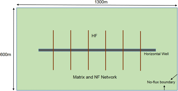
Geometric model of the fractured shale gas reservoir
-
3.
Flow is sequential from one medium to another: from matrix to natural fractures to hydraulic fractures.
-
4.
The desorption of adsorbed gas is only considered in matrix, and the Klinkenberg effect exerts influences on both matrix and natural fractures.
-
5.
The rock is incompressible, and the porosity is seen as a constant.
-
6.
The gas is regarded as compressible real gas, and the gas viscosity and gas compressibility factors are both the function of pressure.

The flow equation of matrix
The continuity equation of matrix is given by:
q m is the inter-porosity flow term from matrix to natural fractures, which is expressed as:
where α mf is the shape factor from matrix to natural fractures, A mf represents the interface area between matrix and natural fractures per unit volume, and Lf represent the characteristic length of natural fracture, which can be seen as its average spacing. The natural fracture spacing in the shale formation is generally 0.05–10 m (Bustin et al. 2008).
In the continuity equation of matrix, when considering Klinkenberg effect, the apparent permeability in the kinetic equation shall be adjusted:
And the gas density can be expressed as:
Substituting Eqs. (6)–(10) into Eq. (5), then we obtain:
Taking the transformation we can obtain:
Substituting Eq. (12) into Eq. (11), we obtain:
Equation (13) is final form of the flow equation of matrix system, and its initial and boundary conditions are:
The flow equation of natural fractures
The continuity equation in natural fracture is:
where q f is the flow term from the natural fractures to the hydraulic fractures:
α fF is the shape factor from natural fractures to hydraulic fractures, and it is defined as the interface area of natural fractures and hydraulic fractures per unit volume divided by the characteristic length of hydraulic fracture.
When considering Klinkenberg effect in the natural fractures:
Substituting Eqs. (19) and (20) into Eq. (16), we obtain:
Equation (21) is final form of the flow equation of natural fractures, and its initial and boundary conditions are:
The flow equation of hydraulic fractures
Unlike the matrix and the natural fractures, hydraulic fractures are discretely distributed with a certain spacing over the reservoir; consequently, the flow in the hydraulic fractures is viewed as one-dimensional flow. Moreover, neither the desorption nor the Klinkenberg effect is considered in the hydraulic fractures; thus, its flow equation is:
where q w is the flow term from hydraulic fractures to the horizontal well, V i,j is the volume of the grid at which the hydraulic fractures intersect with the wellbore, and q is the gas production rate. Figure 3 is an illustration of flow in hydraulic fracture grids.

Illustration of flow in hydraulic fractures
Note that q f is the inter-porosity flow from NF to HF and this is applied to all hydraulic fracture grids, because each HF grid receives flow from NF system. q w is the flow term from HF to the horizontal well, it is only applied to the grid where the HF intersects with the horizontal well, and the production rate is assumed to be constant.
Substituting all the related equations into Eq. (24), we obtain the flow equation of hydraulic fractures, followed by its initial and boundary conditions:
So far we have derived the differential equations for the three media [Eqs. (13), (21) and (29)] together with their initial and boundary conditions; therefore, the entire triple-continuum model is established.
Solution of the mathematical model
This triple-continuum model is solved using finite difference approach, and we discretized the differential equations in each medium via implicit scheme. Within the same time step, we first solve the hydraulic fracture equation to obtain the hydraulic fracture pressure p F and then put it into the natural fracture equation to derive p f, and eventually p m is obtained by solving the matrix equation. By substituting p F into Eq. (28), the production rate of each time cycle is calculated.
Based on this solving algorithm, a program is developed for our simulator. In the program, the gas compressibility factor is calculated by iterative calculation and an empirical equation is employed to calculate the gas viscosity. The detailed calculation procedures for gas properties are shown in Appendix A and B.
Model application and discussion
Model validation
To verify the correctness of this model, we compare the gas rate curve obtained from our model with the prediction from an existing model proposed by Wang (2015). Here we neglect the desorption and Klinkenberg effect and set the parameters of the reservoir according to their paper (reservoir length = 100 m, reservoir width = 100 m, HF height = 100 m, HF half length = 40 m, reservoir permeability = 10−3mD, reservoir porosity = 0.1, reservoir initial pressure = 15 MPa, bottom-hole pressure = 5 MPa). Figure 4 presents the result of the comparison.

Contrast between this study and the result proposed by Wang (2015)
From the results, we can notice that the gas rate curve predicted using our model declines slower than the reference curve in the early stage of the production, it may due to the different calculation of the gas compressibility factor and gas viscosity in the program, and after 400 days of production time, the two gas rate curves can match with each other with negligible disparity. Therefore, despite minor difference from the existing model in the early stage, our model is quite reliable in general.
Reservoir description and model setup
A synthetic shale gas reservoir is employed to demonstrate the application of our proposed model. The reservoir is drilled by a horizontal well and followed by multistage fracturing, and the basic parameters of the shale gas reservoir and the horizontal well are listed in Table 1.
This hypothetical shale reservoir is nominally assumed to be 1500 m deep, and a horizontal well with six hydraulic fractures is incorporated in the model. The size of the reservoir is set to be 1300 m × 600 m × 20 m, the grid size is 75 × 33 × 1 in X, Y and Z direction, and the flow on the vertical direction is neglected. The width of the grids containing hydraulic fractures is set to be 2 m, and the mesh size near the fractures and horizontal well is smaller and finer in order to increase the accuracy. The actual width of hydraulic fracture is assumed to be 5 mm; thus, in our numerical model, the effective permeability for HF grids is calculated using the equation: k eff = k F W F/W grid = 20md (Rubin 2010). This synthetic reservoir is set for the following sensitivity analysis, and the model setup maybe moderately adjusted for the convenience of sensitivity analysis.
The influence of meshing size on gas rate
In order to verify the stableness of this mathematical model, the near wellbore meshing size is altered for different simulation processes, and its influence on gas rate is examined and illustrated in Fig. 5.

Production performances for different values of meshing size
As we can see from Fig. 5, although it shows difference between the three curves at the beginning of the simulation, this difference disappears gradually with time elapsing and only small difference can be seen in the later stage of the simulation. Consequently, the gas rate is insensitive to the change of meshing size, which indicates good stableness of the proposed model as well (Wang 2015).
The influence of fracture half-length on gas rate
Using our triple-continuum model, the production of the reservoir is predicted based on four different values of hydraulic fracture half-length (66, 106, 146 and 186 m), and other parameters are set according to Table 1. The results are shown in Fig. 6.

Production performances for different values of hydraulic fracture half-length
The four curves manifest that the gas rate will rise with the increase in the fracture half-length, and this is especially obvious in the beginning of the production. This is due to the fact that the creation of the hydraulic fractures will substantially promote reservoir’s productivity, and longer fracture half-length can better communicate with the natural fractures, providing a larger pressure drop area which can attract more fluid influx from unstimulated area (Raghavan et al. 1997; Jiang et al. 2014).
However, if we quantitatively analyze the difference between these curves in the later stage of production, we can see: When the fracture half-length increases from 66 to 106 m, then to 146 m and finally to 186 m, the increments of gas rate are about 3500, 3200 and 2400 m3, respectively; thus, the positive effect of hydraulic fracturing stimulation is becoming less apparent. This is because longer HF half length can only provide faster drop of average reservoir pressure, after the pressure drop spreads to the boundary for a long time, the produced gas mainly comes from the desorption gas in matrix, and gas rate mainly depends on matrix permeability. Consequently, the effect of longer HF half length would not be obvious anymore.
The influence of fracture spacing on gas rate
Three different values of hydraulic fracture spacing (100, 140 and 180 m) are selected for the comparison in this case, but the length of the horizontal well is kept constant as 800 m, and the other parameters are set according to Table 1. The production decline curves and cumulative production curves are both shown in Fig. 7.

Production performances for different values of hydraulic fracture spacing
It can be noticed that smaller hydraulic fracture spacing leads to higher gas rate, and the differences are almost 4000 m3. Smaller hydraulic fracture spacing can increase the volume of the stimulated zone near the horizontal well and better communicate with the local natural fractures (Sun and David 2015), thus more effectively enhance the recovery. But we should not neglect that when the length of the horizontal section is fixed, smaller hydraulic fracture spacing indicates the larger amount of hydraulic fractures, in other words, higher cost for the fracturing process. Therefore, there exists an optimal hydraulic fracture spacing economically.
The influence of desorption on gas rate
Langmuir volume V L is an important parameter in the simulation of shale gas reservoir, and it is defined as maximum amount of adsorbed gas per unit volume of rock at a given temperature. To investigate how the desorption effect will affect the gas rate, the Langmuir volume is changed from 0 to 2 cm3/cm3 (V L = 0 indicates neglecting desorption), and different extents of influence are presented schematically in Fig. 8.

Production performances for different values of Langmuir volume
It is evident that the black curve (V L = 0) is much lower than the other three curves, which suggests that the desorption effect will greatly increase the productivity of the reservoir. The adsorbed gas provides about 25 % of the total recovery in the later stage of production. In addition, when V L increases from 0.2 to 2 cm3/cm3, both the production decline curves and the cumulative production curves will rise with small extents. Its reason is that when the reservoir pressure decreases with production, the shale gas in the matrix will continuously desorb from the surface of the matrix pore, and the desorbed gas will feed the natural fractures and the hydraulic fractures, thus enhancing the productivity. Consequently, the gas rate will decline more slowly with larger Langmuir volume.
Apart from Langmuir volume, another important parameter in Langmuir equation is the Langmuir pressure p L, and it represents the pressure at which the adsorbed gas content equals to V L/2. Here Langmuir pressure is changed from 5 to 15 MPa, and the contrast of the simulation results is shown in Fig. 9.

Production performances for different values of Langmuir pressure
It can be observed that the production rate is enhanced when Langmuir pressure grows higher, because the Langmuir pressure indicates the difficulty of the gas desorption, higher Langmuir pressure indicates easier gas desorption in matrix (Liu et al. 2015); thus, the gas rate would decline more slowly. However, the three curves are very close to each other showing very small differences (only 700 m3/day compared to about 18,000 m3/day), which means the production is insensitive to the change of Langmuir pressure.
The influence of Klinkenberg effect on gas rate
Figure 10 demonstrates the influence of Knudsen effect on the gas rate, and we can notice that the gas rate will increase when considering Klinkenberg effect. When the radius of the gas flow path is very small, the gas apparent permeability is greatly increased by Klinkenberg effect, thus enhancing the productivity. In addition, when the pressure drops down, the Klinkenberg effect would become more obvious.

Production performances for different values of Langmuir pressure
In order to gain an insight into the Klinkenberg effect, the apparent permeability is predicted using our simulator and permeability prediction is made on one grid which experiences significant pressure change during the simulation. The alteration of matrix apparent permeability and natural fracture apparent permeability is presented in Fig. 10.
From Fig. 11 we can see that the matrix apparent permeability becomes 4–8 times of its initial permeability, whereas the natural fracture apparent permeability becomes only 1.1 times of its initial permeability. In conclusion, the Klinkenberg effect exerts great influence on matrix but very small influence on natural fracture. The reason is that the pore radius and the intrinsic permeability in matrix are smaller than that in natural fracture system; thus, from the formula introduced in 2.2 we know that the Klinkenberg factor b in matrix is larger, resulting in more significant influence of Klinkenberg effect.

Permeability predictions for the two media
Conclusions
The shale gas experiences many different spatial scales during its flow from the reservoir to the wellbore, resulting in different flow mechanisms. The proposed triple-continuum model can better represent this feature and can simulate the production performance of shale gas well more accurately.
The adsorbed gas in place accounts for considerable fraction of gas reserves and recovery, and the desorption effect will greatly enhance the productivity, especially in the later stage of production; thus, desorption should not be neglected.
The Klinkenberg effect will increase the gas rate by increasing the apparent permeability in matrix and natural fracture, and it exerts greater influence on matrix system than natural fracture.
According to our simulator, the gas rate will rise with the increase in meshing size, hydraulic fracture half-length, Langmuir volume and Langmuir pressure, but with the decrease in hydraulic fracture spacing. Nonetheless, the production is insensitive to the change of meshing size and the Langmuir pressure.
Abbreviations
- A mf :
-
Interface area between matrix and natural fracture per unit volume of rock (m−1)
- A fF :
-
Interface area between natural fracture and hydraulic fracture per unit volume of rock (m−1)
- b :
-
Klinkenberg coefficient (MPa)
- b f :
-
Klinkenberg coefficient for natural fracture (MPa)
- b m :
-
Klinkenberg coefficient for matrix (MPa)
- C g :
-
Compressibility (MPa)
- h :
-
Reservoir thickness (m)
- HF:
-
Hydraulic fracture
- k a :
-
Apparent permeability (md)
- k i :
-
Absolute permeability (md)
- k mi :
-
Absolute permeability of matrix (md)
- k ma :
-
Apparent permeability of matrix (md)
- k fi :
-
Absolute permeability of natural fracture (md)
- k fa :
-
Apparent permeability of natural fracture (md)
- k F :
-
Permeability of hydraulic fracture (md)
- L F :
-
Characteristic length of hydraulic fracture (m)
- L f :
-
Characteristic length of natural fracture (m)
- M g :
-
Molecular weight of gas (kg/mol)
- n :
-
Normal direction
- NF:
-
Natural fracture
- p i :
-
Initial reservoir pressure (MPa)
- p w :
-
Bottom-hole flowing pressure (MPa)
- p m :
-
Matrix pressure (MPa)
- p f :
-
Natural fracture pressure (MPa)
- p F :
-
Hydraulic fracture pressure (MPa)
- p L :
-
Langmuir pressure (MPa)
- q ad :
-
Mass flux of the adsorbed gas [kg/(m3 s)]
- q m :
-
Inter-porosity flow from matrix to natural fracture [kg/(m3 s)]
- q f :
-
Inter-porosity flow from natural fracture to hydraulic fracture [kg/(m3 s)]
- q w :
-
Flow term from hydraulic fractures to the horizontal well [kg/(m3 s)]
- q :
-
Gas rate (m3/day)
- Q :
-
Cumulative gas production (m3/day)
- r e :
-
Effective radius of the grid where HF intersects with wellbore (m)
- r w :
-
Wellbore radius (m)
- R :
-
Universal gas constant [8314 Pa m3/(kmol K)]
- S :
-
Skin factor
- t :
-
Time (s)
- T :
-
Reservoir temperature (K)
- v :
-
Velocity in x and y direction (m/s)
- V E :
-
Adsorbed gas content (cm3/cm3)
- V L :
-
Langmuir volume (cm3/cm3)
- V i,j :
-
Volume of a specific grid (m3)
- x :
-
Length in direction parallel to the horizontal well (m)
- y :
-
Length in direction perpendicular to the horizontal well (m)
- Z :
-
Gas compressibility factor (dimensionless)
- α :
-
Inter-porosity flow shape factor (m)
- Δ:
-
Difference operator
- ρ g :
-
Gas density (kg/m3)
- Φ :
-
Porosity (dimensionless)
- μ g :
-
Gas viscosity (mPa s)
- m:
-
Matrix
- f:
-
Natural fractures
- F:
-
Hydraulic fractures
- mf:
-
Matrix to natural fracture
- fF:
-
Natural fracture to hydraulic fracture
- g:
-
Gas
- Γ:
-
Reservoir boundary
References
Abdassah D, Ershaghi I (1986) Triple porosity system for representing naturally fractured reservoirs. SPE Form Eval 1(2):113–127
Al-Ahmadi HA (2010) A triple-continuum model for fractured horizontal wells. M.Sc. Thesis, Texas A&M University, College Station
Al-Ahmadi A, Ershaghi I (1996) Pressure transient analysis of dually fractured reservoirs. SPE J 1(1):93–100
Apaydin OG, Ozkan E, Raghavan R (2012) Effect of discontinuous microfractures on ultratight matrix permeability of a dual-porosity medium. SPE Reserv Eval Eng 15(4):473–485
Bello RO, Wattenbarger RA (2008) Rate transient analysis in naturally fractured shale gas reservoirs. In: Paper SPE 114591 presented at Gas Technology Symposium joint conference at Calgary, Alberta, Canada
Bello RO, Wattenbarger RA (2009) Modeling and analysis of shale gas production with a skin effect. In: Paper CIPC 2009-082 presented at the Canadian International Petroleum Conference, Calgary, Alberta, Canadian
Bello RO, Wattenbarger RA (2010) Multistage hydraulically fractured shale gas rate transient analysis. In: Paper SPE 114591 presented at the SPE North Africa ATCE, Cairo, Egypt
Bustin AM, Bustin RM, Cui X (2008) Importance of fabric on the production of gas shales. In: Presented at unconventional reservoir conference in Colorado, USA
Cheng Y, Dong B (2012) The flow mechanism for the triple-porosity dual-permeability model in shale gas reservoir. Nat Gas Ind 32(9):44–47
Cipolla CL, Lolon EP, Erdle JC (2010) Reservoir modeling in shale gas reservoir. SPE Reserv Eval Eng 13(4):638–653
Curtis ME (2002) Fractured shale gas systems. AAPG Bull 86(11):1921–1938
Drier J (2004) Pressure transient of wells in reservoirs with a multiple fracture networks. M.Sc. Dissertation, Colorado School of Mines
Guo C, Xu J, Wu K, Wei M, Liu S (2015) Study on gas flow through nano pores of shale gas reservoirs. Fuel 143:107–117
Hassan A, Wattenbarger RA (2011) Triple-porosity models: one further step towards capturing fractured reservoir heterogeneity. Paper presented at the SPE/DGS Saudi Arabia Section Technical Symposium and Exhibition held in Al-Khobar, Saudi Arabia, 15–18 May 2011
Hu W, Qu G, Li J et al (2010) The potential and development of Chinese unconventional reservoirs. Eng Sci 26(12):25–29
Huanlin J (1988) The calculation procedure of natural gas viscosity and its computer program. Nat Gas Ind 8(6):81–85
Javadpour F (2009) Nanopores and apparent permeability of gas flow in mud-rocks (shales and siltstone). J Can Pet Technol 48(8):16–21
Jiang R, Wang Y (2014) A new permeability model for the matrix and natural fractures of shale gas reservoir. Nat Gas Geosci 25(6):934–939
Jiang R, Xu J, Sun Z, Guo C, Zhao Y (2014) Rate transient analysis for multistage fractured horizontal well in tight oil reservoirs considering stimulated reservoir volume. Math Probl Eng. doi:10.1155/2014/489015
Li Y (2009) The Discussion about the measurement of shale gas reserve. Nat Gas Geosci 20(3):466–470
Li F, Wang M, Li W (2015) Pore characteristics of different types of shale in china. Acta Geol Sin 89(supp.):51–54 (English Edition)
Liu H, Hong X, Yu Y (1993) The calculation of gas deviation factor using RKS method (In Chinese). Compress Technol 6:25–27
Liu M, Xiao C, Wang Y et al (2015) Sensitivity analysis of geometry for multi-stage fractured horizontal wells with consideration of finite-conductivity fractures in shale gas reservoirs. J Nat Gas Sci Eng 22:182–195
Lu XC, Li FC, Watson AT (1995) Adsorption studies of natural gas storage in devonian shales. SPE Form Eval 10(2):109–113
Montgomery SL, Jarvie DM, Bowker KA et al (2005) Mississippian Barnett Shale, Fort Worth basin, north-central Texas: gas shale play with multi trillion cubic foot potential. AAPG Bull 89(2):155–175
Ozcan O, Sarak H, Ozkan E et al (2014) A trilinear flow model for a fractured horizontal well in a fractal unconventional reservoir. In: Paper presented at the SPE ATCE, Amsterdam, The Netherlands
Ozkan E, Brown ML, Raghavan RS et al (2009) Comparison of fractured horizontal well performance in conventional and unconventional reservoirs. In: Paper SPE 121290 presented at the SPE Regional Meeting, San Jose, CA
Ozkan E, Raghavan RS, Apaydin OG et al (2010) Modeling of fluid transfer from shale matrix to fracture network. In: Present at ATCE, Lima, Peru
Raghavan R, Chen C, Agarwal B (1997) An analysis of horizontal wells intercepted by multiple fractures. SPE J 2(3):235–245
Rubin B (2010) Accurate simulation of non-darcy flow in stimulated fractured shale gas formations. In: Paper SPE 132193 presented at SPE Western Regional Meeting, Anaheim, 27–29 May
Sarma P, Aziz K (2006) New transfer functions for simulation of naturally fractured reservoirs with dual-porosity models. SPE J 328–340
Sheng M, Li G, Shah SN et al (2012) Extended finite element modeling of multi-scale flow in fractured shale gas reservoirs. SPE ATCE, San Antonio
Sondergeld CH, Ambrose RJ, Rai CS (2010) Micro-structural studies of gas shales. In: Unconventional Gas Conference, Pittsburgh, Pennsylvania, USA
Sun J, David S (2015) Optimization-based unstructured meshing algorithms for simulation of hydraulically and naturally fractured reservoirs with variable distribution of fracture aperture, spacing, length, and strike. SPE Reservoir Eval Eng 18(4):463–480
Sun J, David S, Huang C (2016) Grid-sensitivity analysis and comparison between unstructured perpendicular bisector and structured tartan/local-grid-refinement grids for hydraulically fractured horizontal wells in eagle ford formation with complicated natural fractures. SPE J. doi:10.2118/177480-PA
Wang Y (2015) A dual-continuum discrete fracture modelling approach for numerical simulation of production from unconventional plays. In: Paper SPE-178749-STU presented at the SPE ATCE, Houston, Texas, USA
Wu Y, Karsten P, Peter P (1998) Gas flow in porous media with klinkenberg effects. Transp Porous Media 32(6):117–137
Wu Y, Kang Z, Zhang W et al (2009) A triple-continuum model for production in tight fractured reservoirs. In: Paper SPE 118944 presented at the SPE Hydraulic Fracturing Technology Conference, The Woodlands, Texas, USA
Xu J, Guo C, Wei M, Jiang R (2015) Production performance analysis for composite shale gas reservoir considering multiple transport mechanisms. J Nat Gas Sci Eng 26:382–395
Yao J, Sun H, Huang Z et al (2013) Key mechanical problems in the development of shale gas reservoirs (in Chinese). Sci Sin-Phys Mech Astron 43(12):1527–1547
Zhu Q, Zhang L (2013) The production decline analysis using a triple continuum model considering natural-fractures. Sci Technol Eng 13(29):8595–8599
Author information
Authors and Affiliations
Corresponding author
Appendices
Appendix 1: Calculation for gas compressibility factor Z
For the convenience of programming, here we chose RKS method (Liu et al. 1993), and for the calculation of gas compressibility factor Z, the procedure is shown as follows:
where
w is the acentric factor and 0.3 is always adopted (Liu et al. 1993). Based on the equations mentioned above, we can obtain the Z factor using iterative calculation.
Appendix 2: Calculation for gas viscosity
As for the calculation of gas viscosity, we adopt the empirical equation proposed by Huanlin (1988); following equations are the procedure.
where
μ g,0.1 means the gas viscosity under standard conditions, here we adopt 0.013 mPa s. So for the given temperature and pressure, we can calculate the gas viscosity based on above equations.
Rights and permissions
Open Access This article is distributed under the terms of the Creative Commons Attribution 4.0 International License (http://creativecommons.org/licenses/by/4.0/), which permits unrestricted use, distribution, and reproduction in any medium, provided you give appropriate credit to the original author(s) and the source, provide a link to the Creative Commons license, and indicate if changes were made.
About this article

Cite this article
Zhang, W., Xu, J. & Jiang, R. Production forecast of fractured shale gas reservoir considering multi-scale gas flow. J Petrol Explor Prod Technol 7, 1071–1083 (2017). https://doi.org/10.1007/s13202-016-0281-3
Received:
Accepted:
Published:
Issue Date:
DOI: https://doi.org/10.1007/s13202-016-0281-3