A study of plithogenic graphs: applications in spreading coronavirus disease (COVID-19) globally

Abstract

During the last two decades, the world has experienced three major outbreaks of Coronaviruses, namely severe acute respiratory syndrome (SARS- CoV), middle east respiratory syndrome (MERS-CoV), and the current ongoing pandemic of severe acute respiratory syndrome 2 (SARS-CoV-2). The SARS-CoV-2 caused the disease known as Coronavirus Disease 2019 (COVID-19). Since its discovery for the first time in Wuhan, China, in December 2019, the disease has spread very fast, and cases have been reported in more than 200 countries/territories. In this study, the idea of Smarandache’s pathogenic set is used to discuss the novel COVID-19 spread. We first introduced plithogenic graphs and their subclass, like plithogenic fuzzy graphs. We also established certain binary operations like union, join, Cartesian product, and composition of pathogenic fuzzy graphs, which are helpful when we discuss combining two different graphs. In the end, we investigate the spreading trend of COVID-19 by applying the pathogenic fuzzy graphs. We observe that COVID-19 is much dangerous than (MERS-CoV) and (SARS-CoV). Moreover, as the SARS-CoV and MERS-CoV outbreaks were controlled, there are greater chances to overcome the current pandemic of COVID-19 too. Our model suggests that all the countries should stop all types of traveling/movement across the borders and internally too to control the spread of COVID-19. The proposed model also predicts that in case precautionary measures have not been taken then there is a chance of severe outbreak in future.

1 Introduction

Brief history of COVID-19: In December 2019, Wuhan Health Commission reported a cluster of pneumonia cases of unknown etiology. The pathogen was identified as a novel coronavirus. Later on, World Health Organization named the virus severe acute respiratory syndrome coronavirus (SARS-CoV-2) and caused the disease known as Coronavirus Disease (COVID-19). Since discovering COVID-19 in Wuhan, China, the cases have been reported in more than 200 countries/ territories. As of 01 April 2020 (02:55 PM Nanjing time), a total of 754,948 confirmed cases of COVID-19 have been reported worldwide, with 36,571 deaths. The highest number of cases has been reported in the United States of America 140,640 cases, Italy 101,739 cases, Spain 85,195 cases, China 82,545 cases, Germany 61,913 cases, Iran 44,606 cases, France 43,977 cases, The United Kingdom 22,145 cases, Switzerland 15,412 cases, Belgium 11,899 cases, Netherlands 11,750 cases, Turkey 10,827 cases, and other countries (WHO 2020) . Initially, COVID-19 had a zoonotic basis, which was then spread through the human interaction (Ahmad et al. 2020). Being a novel coronavirus, initially, its etiology was unknown. Later on, scientists identified it found that it had an incubation period of 14 days. Initial two weeks (14 days) are considered as most dangerous concerning the spread of disease (Rodriguez-Morales et al. 2020). Travelers without test/diagnosis were found to be the primary source of infections. For more details we refer the reader (Khan et al. 2021).

Mathematical set’s theory: For handling certain drawbacks of crisp set (CS) theory, Zadeh (1996) introduced fuzzy set (FS) theory. Fuzzy systems have been used successfully for many years in problems involving uncertainty, vagueness, ambiguity, and imprecision of state. Further, Zadeh (1975) extended fuzzy sets (FS) to interval-valued fuzzy sets in which values of membership are intervals instead of real numbers between 0 and 1. Interval-valued fuzzy sets (IVFS) provide precise results of uncertainty than fuzzy sets (FS). Another researcher Atanassov (Atanassove, 1986) , introduced membership and non-membership and gave the idea of the intuitionistic fuzzy set (IFS). It generalized the idea of Zadeh’s fuzzy sets. Jun et al. (2010) gave the idea of cubic sets by combining interval-valued fuzzy sets and fuzzy sets. Cubic sets have many applications in many directions (Jun et al. 2011, 2012). Smarandache extended the idea of Atanassov and gave the concept of neutrosophic set (NS) (Smarandache 1999, 2005). Further Wang et al. (2005) introduced interval valued neutrosophic sets (INS). In 2017, Jun et al. (2017a, b)) presented the idea of neutrosophic cubic sets (NCS) to handle imprecise information. More recently, Smarandache (2017) and Smarandache and Broumi (2018) introduced for the first-time idea of Plithogeny in Philosophy and as its derivatives give the concept of Plithogenic set/logic/probability/statistics in mathematics and engineering. Plithogeny is the origination, formation, development, evolution of new entities and is a connection or combination of theories and ideas in any field. Plithogeny is the dynamics of many opposites, their neutrals and non-opposites, and their organic fusion. The Plithogenic set’s theory generalizes previous theories of fuzzy sets. Smarandache introduce the plithogenic set (as generalization of crisp, fuzzy, intuitionistic fuzzy, and neutrosoph-ic sets), which is a set whose elements are characterized by many attributes’ values. An attribute value v has a corresponding (fuzzy, intuitionistic fuzzy, or neutrosophic) degree of appurtenance d(x, v) of the element x, to the set P, with respect to some given criteria. Plithogenic set theory is being extensively used in various decision-making problems as well as in many other applied fields and for more details we refer the reader (Smarandache 2018a, b, c, d; Gayen et al. 2019; Abdel-Basset et al. 2019; Abdel-Basset and Mohamed 2019; Abdel-Basset et al. 2019; Rana et al. 2019; Gayen et al. 2020). These different versions of sets have been used in the theory of graphs as well; so in the following we provide brief history of graphs.

The theory of graphs: The idea of graph theory is used in many fields. Graph theory is the mathematical structure used to design pair-wise relations between objects. It is constructive in solving problems of different fields as they give a clear picture of the problem at hand. The concept of graph theory begins with the problem of Konigsberg bridge problem in 1736. In 1973, Kauffman (1973) introduced the idea of the fuzzy graph. Rosenfeld (1975) developed the concept of fuzzy graph obtaining analogs of several graph-theoretical concepts. Atanassov (1995) extended his concept of fuzzy sets to intuitionistic fuzzy graphs. For more details see Shannon and Atanassov (1994). Bhattacharya (1987), give some remarks on fuzzy graphs. Akram and Dudek (2011) gave the concept of interval-valued fuzzy graph in 2011. For more details of fuzzy graphs, readers are referred to Akram (2012) and Akram et al. (2013) . The idea of neutrosophic graphs was given by Kandasamy et al. (2015) in the book title as neutrosophic graphs. Rashid et al. (2018) give the concept of neutrosophic cubic graphs with real-life applications in industry. For more details see Gulistan et al. (2018, 2019) and Huang et al. (2019).

Contributions and the motivations: The current study is essential and an excellent addition to the current scientific information and data on COVID-19. After the discovery of SARS-CoV-2, a large number of studies have been conducted to study different aspects of the virus and the disease caused like genetics, mode of transmission, epidemiology, immunotherapeutics, diagnosis, treatment, vaccine, etc. However, very little work has been done to study and plot the COVID-19, spreading of the disease, and burden using the Plithogenic graphs and other models. Thus, this study was performed to answer these quarries. This study will help the researchers, scientists, and policymakers. The same models can be used to predict the co-infections and diseases associated with COVID-19. In this study, Smarandache’s plithogenic set is used to introduce the idea of plithogenic graphs and discuss the novel COVID-19 spread. We also established certain binary operations like union, join, Cartesian product, and composition of plithogenic fuzzy graphs, which are helpful when we discuss two different graphs combined. In the end, we used these concepts to find the effects of COVID-19 in other countries. Since it is a mathematical model assessing the spread of COVID-19, it has more to deal with the mathematical results than experimental work. Tthe primary purpose of this article is to develop the new mathematical model of Plithegonic graphs and test them using the real-life application of the spread of COVID-19.

Organization of the paper: In Sect. 1, named “Introduction,” we provided a brief history and basic definitions of the related material used in this paper. Section 2 is named “The proposed Method” we presented the mathematical model of plithogenic fuzzy graphs with some basic operations. In Sect. 3, “Results and analysis,” we discussed two examples related to covid-19 and examined some exciting outcomes of the proposed mathematical model. Comparison analysis is provided in Sect. 4. Finally, we concluded our study in Sect. 5 with some future work.

1.1 Preliminaries

(Smarandache 2017), Plithogeny is the genesis or origination, creation, formation, development, and evolution of new entities from dynamics and organic fusions of contradictory and/or neutrals and/or non-contradictory multiple old entities. At the same time, plithogenic means what is about plithogeny. A plithogenic set P is a set whose elements are characterized by one or more attributes, and each attribute may have many values. Each attribute’s value v has a corresponding degree of appurtenance d(x, v) of the element x, to the set P, with respect to some given criteria. In order to obtain a better accuracy for the plithogenic aggregation operators, a contradiction (dissimilarity) degree is defined between each attribute value and the dominant (most important) attribute value. However, there are cases when such dominant attribute value may not be taken into consideration or may not exist; therefore, it is considered zero by default, or there may be many dominant attribute values. In such cases, either the contradiction degree function is suppressed, or another relationship function between attribute values should be established. The plithogenic aggregation operators (intersection, union, complement, inclusion, equality) are based on contradiction degrees between attributes’ values, and the first two are linear combinations of the fuzzy operators’ t-norm and t-conorm. Plithogenic set is a generalization of the crisp set, fuzzy set, intuitionistic fuzzy set, and neutrosophic set, since these four types of sets are characterized by a single attribute value (appurtenance): which has one value (membership)—for the crisp set and fuzzy set, two values (membership, and nonmembership)—for intuitionistic fuzzy set, or three values (membership, nonmembership, and indeterminacy)—for the neutrosophic set. So we first provide the defintions of fuzzy set, intuitionistic fuzzy set and neutrosophic set.

Definition 1

(Zadeh 1996) Let S be a universe of discourse then the set

$$\begin{aligned} F_{S}=\{<x,\lambda _{T}(x)>:x\in S\} \end{aligned}$$

(1)

is called the fuzzy set where $\lambda _{T}:S\rightarrow [0,1]$ are truth (membership value), such that $0\le \lambda _{T}(x)\le 1.$

Definition 2

(Atanassov 1986) Let S be a universe of discourse then the set

$$\begin{aligned} I_{S}=\{<x,\lambda _{T}(x),\lambda _{F}(x)>:x\in S\} \end{aligned}$$

(2)

is called the intuitionistic fuzzy set where $\lambda _{T},\lambda _{F}:S\rightarrow [0,1]$ are truth and falsity membership degrees respectively and $0\le \lambda _{T}(x)+\lambda _{F}(x)\le 1.$

Definition 3

(Smarandache 1999) Let S be a universe of discourse then the set

$$\begin{aligned} N_{S}=\{<x,\lambda _{T}(x),\lambda _{I}(x),\lambda _{F}(x)>:x\in S\} \end{aligned}$$

(3)

is the neutrosophic set where $\lambda _{T},\lambda _{I},\lambda _{F} :S\rightarrow [0,1]$ are truth, indeterminancy and falsity membership degrees respectively and $0\le \lambda _{T}(x)+\lambda _{I}(x)+\lambda _{F}(x)\le 3.$

(Smarandache 2017) Plithogenic set is a generalization of the crisp set, fuzzy set, intuitionistic fuzzy set, and neutrosophic set, since these four types of sets are characterized by a single attribute (appurtenance): which has one value (membership)—for the crisp set and for fuzzy set, two values (membership, and nonmembership)—for intuitionistic fuzzy set, or three values (membership, nonmembership, and indeterminacy)—for neutrosophic set.

Definition 4

(Smarandache 2017) Let S be a universal set and $P\subseteq S$. A plithogenic set denoted as $P_{S}$ is defined as

$$\begin{aligned} P_{S}=(P,\chi ,P_{\chi },p_{df},p_{_{CF}}), \end{aligned}$$

(4)

where $\chi$ is an appurtenance or attribute, $P_{\chi }$ is corresponding range of attribute’s value, $p_{df}:P\times P_{\chi }\rightarrow [0,1]^{s}$ is the degree of appurtenance function (DAF) and $p_{_{CF} }:P_{\chi }\times P_{\chi }\rightarrow [0,1]^{t}$ is the corresponding degree of contradiction function (DCF) which will satisfy following axioms: for all $\left( a,b\right) \in P_{\chi }\times P_{\chi }$; $p_{_{Cf}}\left( a,a\right) =0$ and $p_{_{Cf}}\left( a,b\right) =p_{_{Cf}}\left( b,a\right) .$ Here $s,t\in \{1,2,3\}.$ For $s=t=1,$ $P_{S}$ is called plithogenic fuzzy set and is denoted by $P_{FS},$ also for $s=2;t=1$; $P_{S}$ is called plithogenic intuitionistic fuzzy set and is denoted by $P_{IFS}$ and for $s=3;t=1$ $P_{S}$ is called plithogenic neutrosophic set and is denoted by $P_{NS}$.

Definition 5

(Rosenfeld 1975) A fuzzy graph with set of vertices V is defined to be a pair $G=(\theta ,\delta ),$where $\theta$ is a fuzzy function in V and $\nu$ is a fuzzy function in $E\subseteq V$ $\times V$, such that

$$\begin{aligned} \delta (xy)\le \min \left\{ \left( \theta (x),\theta (y)\right) \right\} \ \text {for all }xy\in E. \end{aligned}$$

(5)

We call $\theta$ the fuzzy vertex function of V, $\nu$ the fuzzy edge function of E,  respectively. Note that $\nu$ is a symmetric fuzzy relation on $\theta$. Thus, $G=(\theta ,\nu )$ is a fuzzy graph of $G^{*}=(V,E)$ if $\delta (xy)\le \min (\theta (x),(y))$ for all $xy\in E$.

Definition 6

(Atanassov 1995) An intuitionistic fuzzy graph is of the form $G_{IF} =(\theta _{V},\delta _{E})$ where $\theta _{V}=(\theta _{TV},\theta _{FV})$ which consists of degree of membership function $\theta _{TV}:V\rightarrow [0,1]$ for vertices and degree of non-membership function $\theta _{FV}:V\rightarrow [0,1]$ for vertices. Also $\delta _{E}=(\delta _{TE},\delta _{FE})$ consists of degree of membership function $\delta _{TE}:E\rightarrow [0,1]$ for edges and degree of non-membership function $\delta _{FE}:E\rightarrow [0,1]$ for edges such that

$$\begin{aligned} \delta _{TE}(xy)\le & {} \min \{\theta _{TV}(x),\theta _{TV}(y)\}, \end{aligned}$$

(6)

$$\begin{aligned} \delta _{FE}(xy)\ge & {} \max \{\theta _{FV}(x),\theta _{FV}(y)\}, \end{aligned}$$

(7)

$0\le \delta _{TE}(xy)+\delta _{FE}(xy)\le 1,$ for all$xy\in E.$

Definition 7

(Gulistan et al. 2018) Let $G^{*}=(V,E)$ be a crisp graph. By a neutrosophic graph of $G^{*}$, we mean a pair $G_{N}=(P,Q)$, where $P=(\theta _{T},\theta _{I},\theta _{F})$ is neutrosophic set of vertex set V and $Q=(\delta _{T},\delta _{I},\delta _{F})$ is neutrosophic set of edge set E; such that

$$\begin{aligned} \delta _{T}(xy)\le & {} \min \{\theta _{T}(x),\theta _{T}(y)\}, \end{aligned}$$

(8)

$$\begin{aligned} \delta _{I}(xy)\le & {} \min \{\theta _{I}(x),\theta _{I}(y)\}, \end{aligned}$$

(9)

$$\begin{aligned} \delta _{F}(xy)\ge & {} \max \{\theta _{F}(x),\theta _{F}(y)\} \end{aligned}$$

(10)

for all $x,y\in V$ and $xy\in E.$

Based on the above literate, it is quite natural to extend the notions of neutrosophic graphs in the environment of plithogenic set as under,

2 The proposed method (plithogenic fuzzy graphs)

In this section, we define a more general class of fuzzy graphs known as plithogenic graphs. We also discuss plithogenic fuzzy graphs and their basic operations like union, join, cartesian product, and composition.

Definition 8

Let $G^{*}=(V,E)$ be a crisp graph. A plithogenic graph denoted as $P_{G}$ is defined as $P_{G}=(P_{M},P_{N})$ where $P_{M}=(M,\mu ,M_{\mu },\alpha _{df},\alpha _{Cf})$ is plithogenic set for vertices; where $M\subset V$, $\mu$ is an attribute, $M_{\mu }$ is the corresponding range of attribute values such that $\alpha _{df}:M\times M_{\mu }\rightarrow \left[ 0,1\right] ^{s}$ is the degree of appurtenance function (DAF) for vertices defined as $\alpha _{df}(x$, $a)\in \left[ 0,1\right] ^{s}.$and $\alpha _{Cf}:M_{\mu }\times M_{\mu }\rightarrow \left[ 0,1\right] ^{t}$is degree of contradiction function (DCF) for vertices. Also $P_{N}=(N,\nu ,N_{\nu },\beta _{df},\beta _{Cf})$ is plithogenic set for edges, where $N\subset E$ , $\nu$ is some attribute, $N_{\nu }$ is the corresponding range of attribute values such that $(M_{\mu },N_{v})$ is a graph with vertices $M_{\mu \text { }}$ and edges $N_{v}$. Also $\beta _{df}:N\times N_{\nu }\rightarrow \left[ 0,1\right] ^{s}$ is the degree of appurtenance function for edges and $\beta _{Cf}:N_{\nu }\times N_{\nu }\rightarrow \left[ 0,1\right] ^{t}$ is degree of contradiction function for edges. Then $P_{G}$ is plithogenic graph iff for all $(x,a) \& (y,b)\in M\times M_{\mu };$

$$\begin{aligned} \beta _{df}((x,a)(y,b))\le & {} \min \{\alpha _{_{df}}(x,a),\alpha _{_{df}}(y,b)\}, \end{aligned}$$

(11)

$$\begin{aligned} \beta _{Cf}((a,b)(c,d))\le & {} \min \{\alpha _{Cf}((a,b),\alpha _{Cf}(c,d)\} \end{aligned}$$

(12)

for all $((a,b)(c,d))\in N_{\nu }\times N_{\nu },$ where $\beta _{Cf}((a,b)(a,b))=0$ as $\alpha _{Cf}((a,a)=0=\alpha _{Cf}(b,b)).$ Here $s,t\in \{1,2,3\}.$

Here we discuss a subclass of plithogenic graphs known as plithogenic fuzzy graphs.

Definition 9

If we take $s=t=1$ in the Definition 8, then we define the plithogenic fuzzy graph $P_{FG}$ as follows; A plithogenic fuzzy graph of a crisp graph $G^{*}=(V,E)$ denoted by $P_{FG}\$is defined as $P_{FG}=(P_{FM},P_{FN})$ where $P_{FM}=(M,\mu ,M_{\mu },\alpha _{Fdf}, \alpha _{Fcf})$ is plithogenic fuzzy set $P_{FM}$ for vertices; where $M\subset V$, $\mu$ is an attribute, $M_{\mu }$ is the corresponding range of attribute values such that $\alpha _{Fdf}:M\times M_{\mu }\rightarrow \left[ 0,1\right]$ is the fuzzy degree of appurtenance function (FADF) for vertices defined as $\alpha _{Fdf}(x,b)\in \left[ 0,1\right]$and $\alpha _{Fcf}:M_{\mu }\times M_{\mu }\rightarrow [0,1]$ is fuzzy degree of contradiction function (FDCF) for vertices. Also $P_{FN}=(N,\nu ,N_{ \nu },\beta _{Fdf},\beta _{Fcf})$ is plithogenic fuzzy set $P_{FN}$ for edges; where $N\subset E$, $\nu$ is some attribute, $N_{\nu }$ is the corresponding range of attribute values such that $\beta _{Fdf}:N\times N_{\nu }\rightarrow \left[ 0,1\right]$ is the (FDAF) for edges defined as $\beta _{Fdf}((x,a)(y,b)=\beta _{Fdf}(xy,ab)\in \left[ 0,1\right] .$and $\beta _{Fcf}:N_{\nu }\times N_{\nu }\rightarrow [0,1]$ is (FDCF) for edges such that $(M_{\mu },N_{v})$ is a graph with $M_{\mu }$ as vertices and $N_{v}$ as edges. Then $P_{FG}$ is plithogenic fuzzy graph iff for all $(x,a) {\text {and}} (y,b)\in M\times M_{\mu };$

$$\begin{aligned} \beta _{Fdf}((x,a)(y,b))&\le \min \{ \alpha _{Fdf}(x,a),\alpha _{Fdf}(y,b)\}, \nonumber \\ \beta _{Fcf}((a,b)(c,d))&\le \min \{ \alpha _{Fcf}(a,b),\alpha _{Fcf}(c,d)\} \text { } \end{aligned}$$

(13)

for all $((a,b),(c,d))\in N_{\nu }\times N_{\nu }.$ Since $\beta _{Fcf}((a,b)(a,b))=0$ as $\alpha _{Fcf}(a,a)=0=\alpha _{Fcf}(b,b).$

Example 1

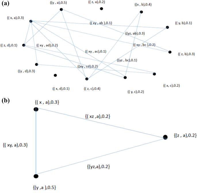
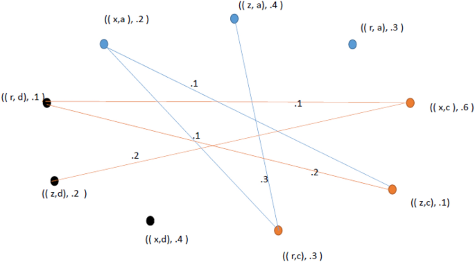
Let $G^{*}=(V,E)$ be a crisp graph, where V isthe set of all countries where people are suffering from the coronavirus (COVID-19). Let $M=\{x,y,z\}\subset V$ be any three countries under consideration and $M_{\mu }=\{a=$ fever,  $b=$ cough, $c=$ dyspnoea, $d=$ fatigue$\}$ is corresponding range for some attribute $\mu =$ typical symptoms and $N=\{xy,yz,xz\}$ be their relationship with each other and $N_{v}$ be reasons for spreading , then $(M_{\mu },N_{v})$ is a graph with vertices $M_{\mu }=\{a,b,c,d\}$ and edges $N_{v}=\{ab,bc,cd,ac,ad\}.$ Also let $\alpha _{Fdf}:M\times M_{\mu }\rightarrow \left[ 0,1\right]$ and $\alpha _{FCf}:M_{\mu }\times M_{\mu }\rightarrow [0,1]$ is the FDAF and FDCF for vertices defined as in Table 1(i) and (ii).

Here second column of FDAF in Table 1 shows that $30\%$ people get effected from fever, $40\%$ effected from cough, $20\%$ from dyspnoea and $10\%$ from fatigue, which then converted into coronavirus (COVID-19) in a country x. Similarly we have observations for country y and for counyrty z. Also the FDAF and FDCF for edges is defined as in Table 2(i) and (ii).

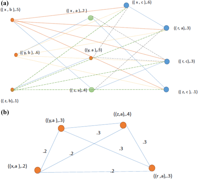
Using the Definition 9, it is obvious that $P_{FG}$ is a plithogenic fuzzy graph as shown in Fig. 1a.

Table 1 (i) FDAF for vertices and (ii) FDCF for vertices

Table 2 (i) FDAF for edges and (ii) FDCF for edges

Fig. 1

a A plithogenic fuzzy graph $\mathrm {P_FG}$. b) A fuzzy graph

Remark 1

If we have only one attribute i.e, fever or cough, then plithogenic fuzzy graph provided in Fig. 1a reduces to fuzzy graph as shown in Fig. 1b

so by doing so we have lost a lot of information.

2. If we increase the range of attributes, we may get more reliable information, which is main theme of plithogenic sets.

Fig. 2

A plithogenic fuzzy graph $\mathrm {P}_\mathrm{{FG}1}$

2.1 Union of plithogenic fuzzy graphs

Definition 10

Let $G_{1}^{*}=(V_{1},E_{1})$ and $G_{2}^{*}=(V_{2},E_{2})$ be any two crisp graphs. Also suppose that $P_{FG_{1}}$and $P_{FG_{2}}$ be any two plithogenic fuzzy graphs such that $P_{FG_{1}}=(P_{FM_{1}},P_{FN_{1}}),$ where $P_{FM_{1}}=(M_{1},\mu _{1},M_{ \mu _{1}},\alpha _{1}{}_{_{Fdf}},\alpha _{1}{}_{_{FCf}})$ and $P_{FN_{1}}=(N_{1},\nu _{1},N_{\nu _{1}},\beta _{1}{}_{_{Fdf}},\beta _{1}{}_{_{_{FCf}}}).$ Also $P_{FG_{2}}=(P_{FM_{2}},P_{FN_{2}})$, where $P_{FM_{2}}=(M_{2},\mu _{2},M_{\mu _{2}},\alpha _{2_{Fdf}}, \alpha _{2}{}_{_{FCf}})$ and $P_{FN_{2}}=(N_{2},\nu _{2},N_{\nu _{2}}, \beta _{2}{}_{_{Fdf}},\beta _{2}{}_{_{FCf}}).$ Then their union is defined as $P_{FG_{1}\cup FG_{2}}=(P_{FM_{1}\cup FM_{2}},P_{FN_{1}\cup FN_{2}})$ where $P_{FM_{1}\cup FM_{2}}=(M_{1}\cup M_{2},\mu _{1}\cup \mu _{2},M_{_{\mu _{1}}}\cup M_{\mu _{2}},(\alpha _{1_{_{Fdf}}}\cup \alpha _{2_{_{Fdf}}}),(\alpha _{1_{FCf}}\cup \alpha _{2_{FCf}}))$ is union of plithogenic sets for vertices. Here $\left( M_{1}\cup M_{2}\right) \subset \left( V_{1}\cup V_{2}\right)$, $\mu _{1}\cup \mu _{2}$ is an attribute, $M_{\mu _{1}}\cup M_{\mu _{2}}$ is the corresponding range of attribute values and $\alpha _{1_{_{Fdf}}}\cup \alpha _{2_{Fdf}}:\left( M_{1}\cup M_{2})\times (M_{\mu _{1}}\cup M_{\mu _{2}}\right) \rightarrow \left[ 0,1\right]$ is the DAF for vertices such that $(\alpha _{1_{_{Fdf}}}\cup \alpha _{2_{_{Fdf}}})(x,x_{\mu })\in \left[ 0,1\right]$ and is defined as

• 1. $(\alpha _{1_{_{Fdf}}}\cup \alpha _{2_{_{Fdf}}})(x,x_{_{\mu }})=\alpha _{1}{}_{_{Fdf}}(x,x_{_{\mu }})$ if $\left( x,x_{_{\mu }}\right) \in \left( M_{1}\times M_{\mu _{1}}\right) \backslash \left( M_{2}\times M_{\mu _{2}}\right) ,$

• 2. $\alpha _{1_{_{Fdf}}}\cup \alpha _{2_{_{Fdf}}})(x,x_{_{\mu }})=\alpha _{2_{Fdf}}(x,x_{_{\mu }})$ if $\left( x,x_{_{\mu }}\right) \in \left( M_{2}\times M_{\mu _{2}}\right) \backslash \left( M_{1}\times M_{\mu _{1}}\right) ,$

• 3. $(\alpha _{1_{_{Fdf}}}\cup \alpha _{2_{_{Fdf}}})(x,x_{_{\mu }})=\max \{ \alpha _{1}{}_{_{Fdf}}(x,x_{_{\mu }}),\alpha _{2_{Fdf}}(x,x_{_{\mu }})\},$

  if $\left( x,x_{_{\mu }}\right) \in \left( M_{1}\times M_{\mu _{1}}\right) \cap \left( M_{2}\times M_{\mu _{2}}\right)$ and $(\alpha _{1_{FCf}}\cup \alpha _{2_{FCf}}):(M_{\mu _{1}}\cup M_{\mu _{2}})\times \left( M_{\mu _{1}}\cup M_{\mu _{2}}\right) \rightarrow \left[ 0,1\right]$ is fuzzy degree of contradiction function (FDCF) for vertices, such that $\left( \alpha _{1}\cup \alpha _{2}\right) _{_{FCf}}(x_{i\mu },x_{i\mu })=0$ for all $\left( x_{i\mu },x_{i_{\mu }}\right) \in (M_{\mu _{1}}\cup M_{\mu _{2}})\times \left( M_{\mu _{1}}\cup M_{\mu _{2}}\right)$ and $(\alpha _{1_{FCf}}\cup \alpha _{2_{FCf}})(x_{i\mu },x_{j_{\mu }})=\left( \alpha _{1_{FCf}}\cup \alpha _{2_{FCf}}\right) (x_{j\mu },x_{i_{\mu }})$ for all $\left( x_{i\mu },x_{j_{\mu }}\right) \in (M_{\mu _{1}}\cup M_{\mu _{2}})\times \left( M_{\mu _{1}}\cup M_{\mu _{2}}\right) .$ Also $P_{_{FN_{1}\cup FN_{2}}}=(N_{1}\cup N_{2},\nu _{1}\cup \nu _{2},\left( N_{\nu _{1}}\cup N_{\nu _{2}}\right) ,(\beta _{1_{_{Fdf}}}\cup \beta _{2_{Fdf}}),(\beta _{1_{FCf}}\cup \beta _{2_{FCf}}))$ is union of plithogenic fuzzy sets for edges, where $\left( N_{1}\cup N_{2}\right) \subset \left( E_{1}\cup E_{2}\right)$, $\nu _{1}\cup \nu _{2}$ is the attribute, $\left( N_{\nu _{1}}\cup N_{\nu _{2}}\right)$ is the corresponding range of attribute values such that $\left( \beta _{1_{_{Fdf}}}\cup \beta _{2_{_{Fdf}}}\right) :\left( N_{1}\cup N_{2}\right) \times \left( N_{\nu _{1}}\cup N_{\nu _{2}}\right) \rightarrow \left[ 0,1\right]$ is the DAF for edges; and is defined as,

  (iv) $(\beta _{1_{_{Fdf}}}\cup \beta _{2_{_{Fdf}}})\left( (x_{1},x_{1_{\mu }}),(x_{2},x_{_{2\mu }})\right) =\beta _{1_{Fdf}}\left( (x_{1},x_{1_{\mu }}),(x_{2},x_{_{2\mu }})\right)$ if

  $$\begin{aligned} \left( (x_{1},x_{1_{\mu }}),(x_{2},x_{_{2\mu }})\right) \in (N_{1}\times N_{\nu _{1}})\setminus (N_{2}\times N_{\nu _{2}}) \end{aligned}$$

  (v) $(\beta _{1_{_{Fdf}}}\cup \beta _{2_{_{Fdf}}})\left( (x_{1},x_{1_{\mu }}),(x_{2},x_{_{2\mu }})\right) =\beta _{2F_{df}}\left( (x_{1},x_{1_{\mu }}),(x_{2},x_{_{2\mu }})\right)$ if

  $$\begin{aligned} \left( (x_{1},x_{1_{\mu }}),(x_{2},x_{_{2\mu }})\right) \in (N_{2}\times N_{\nu _{2}})\setminus (N_{1}\times N_{\nu _{1}}) \end{aligned}$$

  (vi) $(\beta _{_{1_{Fdf}}}\cup \beta _{2_{_{Fdf}}})\left( (x_{1},x_{1_{\mu }}),(x_{2},x_{_{2\mu }})\right) =\max \left\{ \begin{array}{c} \beta _{1_{Fdf}}\left( (x_{1},x_{1_{\mu }}),(x_{2},x_{_{2\mu }})\right) , \\ \beta _{2_{Fdf}}\left( (x_{1},x_{1_{\mu }}),(x_{2},x_{_{2\mu }})\right) \end{array} \right\}$ if

  $$\begin{aligned} \left( (x_{1},x_{1_{\mu }}),(x_{2},x_{_{2\mu }})\right) \in (N_{1}\times N_{\nu _{1}})\cap (N_{2}\times N_{\nu _{2}}) \end{aligned}$$

  also we have FDCF for edges $(\beta _{1_{FCf}}\cup \beta _{2_{FCf}}):\left( N_{\nu _{1}}\cup N_{\nu _{2}}\right) \times \left( N_{\nu _{1}}\cup N_{\nu _{2}}\right) \rightarrow [0,1]$ such that

  $$\begin{aligned} \left( \beta _{1_{FCf}}\cup \beta _{2_{FCf}}\right) ((a,b)(a,b))=0 \end{aligned}$$

  and

  $$\begin{aligned} \left( \beta _{1_{FCf}}\cup \beta _{2FCf}\right) ((a,b)(c,d))=\left( \beta _{1_{FCf}}\cup \beta _{2_{FCf}}\right) (c,d)((a,b)) \end{aligned}$$

  for all $((a,b)(c,d))\in \left( N_{\nu _{1}}\cup N_{\nu _{2}}\right) \times \left( N_{\nu _{1}}\cup N_{\nu _{2}}\right) .$ Then $P_{FG_{1}\cup FG_{2}}=(P_{FM_{1}\cup FM_{2}},P_{FN_{1}\cup FN_{2}})$ is a plithogenic fuzzy graph iff

  $$\begin{aligned}&(\beta _{1_{_{Fdf}}}\cup \beta _{2_{_{Fdf}}})((x,a)(y,b)) \end{aligned}$$

  (14)
  $$\begin{aligned}\le & {} \min \left\{ \begin{array}{c} \left( (\alpha _{1_{_{Fdf}}}\cup \alpha _{2_{_{Fdf}}})(x,a)\right) , \\ \left( (\alpha _{1_{_{Fdf}}}\cup \alpha _{2_{_{Fdf}}})(y,b)\right) \end{array} \right\} \end{aligned}$$

  (15)

  for all $((x,a)(y,b))\in \left( N_{1}\cup N_{2}\right) \times \left( N_{\nu _{1}}\cup N_{\nu _{2}}\right) ;$ also

  $$\begin{aligned}&((\beta _{1_{FCf}}\cup \beta _{2_{FCf}})((a,b)(c,d))) \end{aligned}$$

  (16)
  $$\begin{aligned}\le & {} \min \left\{ \begin{array}{c} (\alpha _{1_{_{_{FCf}}}}\cup \alpha _{2_{FCf}})(a,b), \\ (\alpha _{1_{_{_{FCf}}}}\cup \alpha _{2_{_{_{FCf}}}})(c,d) \end{array} \right\} \end{aligned}$$

  (17)

  for all $((a,b)(c,d))\in \left( N_{\nu _{1}}\cup N_{\nu _{2}}\right) .$

Example 2

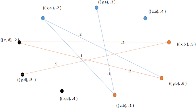
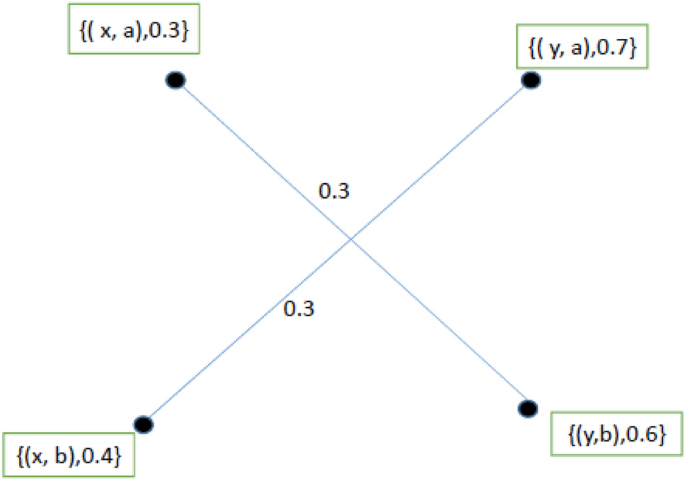
Consider any two plithogenic graphs $P_{FG_{1}}=(P_{FV_{1}},Q_{FE_{1}})$ and $P_{FG_{2}}=(P_{FV_{2}},Q_{FE_{2}})$ of crisp graphs $G_{1}^{*}=(V_{1},E_{1})$ and $G_{2}^{*}=(V_{2},E_{2}),$ where $P_{FV_{1}}=(P_{1},\mu _{1},P_{\mu _{1}},\alpha _{1}{}_{_{Fdf}},\alpha _{1}{}_{_{FCf}}) \&$ $Q_{FE_{1}}=(Q_{1},\nu _{1},Q_{\nu _{1}},\beta _{1}{}_{_{Fdf}},\beta _{1}{}_{_{_{FCf}}})$ such that$(P_{1},Q_{1})$ is a graph with vertices $P_{1}=\{x,y,z\}$ and edges $Q_{1}=\{xy,yz,xz\},(\mu _{1},\nu _{1})$ be an attribute, $(P_{\mu _{1}},Q_{\nu _{1}})$ be a graph with vertices $P_{\mu _{1}}=\{a,b,d\}$ and edges $Q_{\nu _{1}}=\{ab,bd\}.$ Also let $\alpha _{1}{}_{_{Fdf}}:P_{1}\times P_{\mu _{1}}\rightarrow [0,1]$ and $\alpha _{1}{}_{_{FCf}}:P_{\mu _{1}}\times P_{\mu _{1}}\rightarrow [0,1]$ be FDAFand FDCF for vertices defined as

Also $\beta _{1}{}_{_{Fdf}}:Q_{1}\times Q_{\nu _{1}}\rightarrow [0,1]$ and $\beta _{1}{}_{_{_{FCf}}}:Q_{\nu _{1}}\times Q_{\nu _{1}}\rightarrow [0,1]$ be FDAF and FDCF for edges defined as

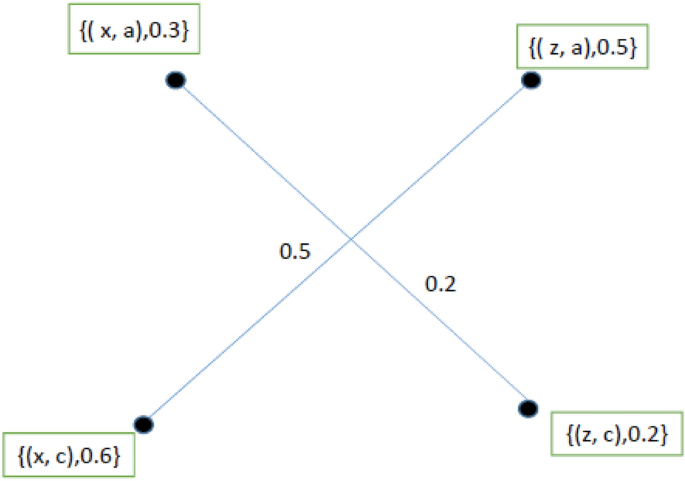
Then using the Definition 9, it is obvious that $P_{FG_{1}}$ is a plithogenic fuzzy graph as shown in Fig. 2, Similarly we have a plithogenic fuzzy graph $P_{FG_{2}};$ with $P_{FV_{2}}=\left( P_{2},\mu _{2},P_{\mu _{2}},\alpha _{2_{Fdf}},\alpha _{2}{}_{_{FCf}}\right)$ & $Q_{FE_{2}}=\left( Q_{2},\nu _{2},Q_{\nu _{2}},\beta _{2}{}_{_{Fdf}},\beta _{2}{}_{_{FCf}}\right)$ such that $(P_{2},Q_{2})$ is a graph with vertices $P_{2}=\{x,z,r\}$ and edges $Q_{2}=\{xz,zr,xr\},(\mu _{2},\nu _{2})$ be an attribute$,(P_{\mu _{2}},Q_{\nu _{2}})$ is a graph with vertices $P_{\mu _{2}}=\{a,c,d\}$ and edges $Q_{\nu _{2}}=\{ac,cd\}.$ Also let $\alpha _{2}{}_{_{Fdf}}:P_{2}\times P_{\mu _{2}}\rightarrow [0,1]$ and $\alpha _{2}{}_{_{FCf}}:P_{\mu _{2}}\times P_{\mu _{2}}\rightarrow [0,1]$ be FDAFand FDCF for vertices defined as

Also $\beta _{2}{}_{_{Fdf}}:Q_{2}\times Q_{\nu _{2}}\rightarrow [0,1]$ and $\beta _{2}{}_{_{_{FCf}}}:Q_{\nu _{2}}\times Q_{\nu _{2}}\rightarrow [0,1]$ be FDAFand FDCF for edges defined as

Then using the Definition 9, it is obvious that $P_{FG_{2}}$ is a plithogenic fuzzy graph as shown in Fig. 3. Then their union is defined as $P_{FG_{1}\cup FG_{2}}=(P_{FV_{1}\cup FV_{2}},Q_{FE_{1}\cup FE_{2}})$ where

$$\begin{aligned} P_{FV_{1}\cup FV_{2}}=\left( \begin{array}{c} P_{1}\cup P_{2},\mu _{1}\cup \mu _{2}, \\ P_{\mu _{1}\cup \mu _{2}},(\alpha _{1_{_{Fdf}}}\cup \alpha _{2_{_{Fdf}}}), \\ (\alpha _{1_{FCf}}\cup \alpha _{2_{FCf}}) \end{array} \right) \end{aligned}$$

and

$$\begin{aligned} Q_{FE_{1}\cup FE_{2}}=\left( \begin{array}{c} Q_{1}\cup Q_{2},\nu _{1}\cup \nu _{2}, \\ Q_{\nu _{1}\cup \nu _{2}},(\beta _{1_{_{Fdf}}}\cup \beta _{2_{_{Fdf}}}), \\ (\beta _{1_{FCf}}\cup \beta _{2_{FCf}}). \end{array} \right) \end{aligned}$$

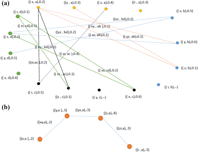
Here we have $P_{1}\cup P_{2}=\{x,y,z,r\}$, $Q_{1}\cup Q_{2}=\{xy,yz,xz,zr,xr\}$ such that $(P_{1}\cup P_{2},Q_{1}\cup Q_{2})$ is a graph, $(\mu _{1}\cup \mu _{2},\nu _{1}\cup \nu _{2})$ is an attribute, $P_{\mu _{1}\cup \mu _{2}}=\{a,b,c,d\}$ is range of attribute for vertices and $Q_{\nu _{1}\cup \nu _{2}}=\{ab,bd,ac,cd\}$ is range of attribute for edges so that $(P_{\mu _{1}\cup \mu _{2}},Q_{\nu _{1}\cup \nu _{2}})$ is a graph. Here $(\alpha _{1_{Fdf}}\cup \alpha _{2_{Fdf}}):(P_{1}\cup P_{2})\times P_{\mu _{1}\cup \mu _{2}}\rightarrow [0,1]$ and $(\alpha _{1_{FCf}}\cup \alpha _{2_{FCf}}):P_{\mu _{1}\cup \mu _{2}}\times P_{\mu _{1}\cup \mu _{2}}\rightarrow [0,1]$ are FDAFand FDCF for vertices defined as in Table 7(i) and (ii).

also $(\beta _{1_{_{Fdf}}}\cup \beta _{2_{_{Fdf}}}):(Q_{1}\cup Q_{2})\times Q_{\nu _{1}\cup \nu _{2}}\rightarrow [0,1]$ and $(\beta _{1_{FCf}}\cup \beta _{2_{FCf}}):Q_{\nu _{1}\cup \nu _{2}}\times Q_{\nu _{1}\cup \nu _{2}}\rightarrow [0,1]$ are FDAFand FDCF for edges and is defined as in Table 8(i) and (ii).

Using the Definition 10, it is obvious that $P_{FG_{1}\cup FG_{2}}$ is a plithogenic fuzzy graph as represented as in Fig. 4a.

Table 3 FDAF and FDCF for vertices of $P_{FG_{1}}$

Table 4 FDAF and FDCF for edges of $P_{FG_{1}}$

Fig. 3

A plithogenic fuzzy graph $\mathrm {P}_\mathrm{{FG}2}$

Table 5 FDAF and FDCF for vertices of $P_{FG_{2}}$

Table 6 FDAF and FDCF for vertices of $P_{FG_{2}}$

Fig. 4

aUnion of two plithogenic fuzzy graphs P_FG1UFG2. b Union of two fuzzy graphs

Table 7 (i) FDAF for vertices of $P_{FG_{1}\cup FG_{2}}$ and (ii) FDCF for vertices of $P_{FG_{1}\cup FG_{2}}$

Table 8 (i) FDAF for edges of $P_{FG_{1}\cup FG_{2}}$and (ii) FDCF for edges of ${P_{FG_{1}\cup FG_{2}}}$

Fig. 5

Plithogenic fuzzy graph P_FG1

Fig. 6

Plithogenic fuzzy graph P_FG2

Remark 2

If we have only one attribute in plithogenic fuzzy graphs $P_{FG_{1}}$and $P_{FG_{2}}$ then union of plithogenic fuzzy graphs provided in Fig. 4a reduces to union of fuzzy graphs as shown in Fig. 4b.

2.2 Join of plithogenic fuzzy graphs

Definition 11

Consider any two plithogenic graphs $P_{FG_{1}}=(P_{FV_{1}},Q_{FE_{1}})$ and $P_{FG_{2}}=(P_{FV_{2}},Q_{FE_{2}})$ as given in Definition 10 of crisp graphs $G_{1}^{*}=(V_{1},E_{1})$ and $G_{2}^{*}=(V_{2},E_{2}).$ We define their join as $P_{FG_{1}+FG_{2}}=(P_{FV_{1}+FV_{2}},Q_{FE_{1}+FE_{2}})$ where $P_{FV_{1}+FV_{2}}=(P_{1}\cup P_{2},\mu _{1}\cup \mu _{2},P_{\mu _{1}\cup \mu _{2}},(\alpha _{1_{_{Fdf}}}+\alpha _{2_{_{Fdf}}}),(\alpha _{1_{FCf}}+ \alpha _{2_{FCf}}))$, $Q_{FE_{1}+FE_{2}}=(Q_{1}\cup Q_{2},\nu _{1}\cup \nu _{2},Q_{\nu _{1}\cup \nu _{2}},(\beta _{1_{_{Fdf}}}+\beta _{2_{_{Fdf}}}),(\beta _{1_{FCf}}+ \beta _{2_{FCf}}))$ and $Q_{FE_{1}\cup FE_{2}}=(Q_{1}\cup Q_{2}\cup Q^{\prime },\nu _{1}\cup \nu _{2},Q_{\nu _{1}\cup \nu _{2}},(\beta _{1_{_{Fdf}}}\cup \beta _{2_{_{Fdf}}}),(\beta _{1_{FCf}}\cup \beta _{2_{FCf}})).$ Here we have $P_{1}\cup P_{2}\subseteq V_{1}\cup V_{2}$, $Q_{1}\cup Q_{2}\subseteq E_{1}\cup E_{2}$ such that $(P_{1}\cup P_{2},Q_{1}\cup Q_{2})$ is a graph, $(\mu _{1}\cup \mu _{2},\nu _{1}\cup \nu _{2})$ is an attribute, $P_{\mu _{1}\cup \mu _{2}}$ is range of attributes for vertices and $Q_{\nu _{1}\cup \nu _{2}}$ is range of attributes for edges so that $(P_{\mu _{1}\cup \mu _{2}},Q_{\nu _{1}\cup \nu _{2}})$ is a graph. Here FDAF for vertices of $P_{FG_{1}+FG_{2}}$ i.e. for $P_{1}\cup P_{2}$ is $(\alpha _{1_{Fdf}}+\alpha _{2_{Fdf}}):(P_{1}\cup P_{2})\times P_{\mu _{1}\cup \mu _{2}}\rightarrow [0,1]$is defined as

$(i)(\alpha _{1_{Fdf}}+\alpha _{2_{Fdf}})(x,x_{\mu })=(\alpha _{1_{Fdf}}\cup \alpha _{2_{Fdf}})(x,x_{\mu })$ if $(x,x_{\mu })\in (P_{1}\cup P_{2})\times P_{\mu _{1}\cup \mu _{2}}$ and FDCF for vertices is $(\alpha _{1_{FCf}}+ \alpha _{2_{FCf}}):P_{\mu _{1}\cup \mu _{2}}\times P_{\mu _{1}\cup \mu _{2}}\rightarrow [0,1]$ such that $(\alpha _{1_{FCf}}+ \alpha _{2_{FCf}})(a,a)=0$ for all $(a,a)\in P_{\mu _{1}\cup \mu _{2}}\times P_{\mu _{1}\cup \mu _{2}}$ and $(\alpha _{1_{FCf}}+\alpha _{2_{FCf}})(a,b)=( \alpha _{1_{FCf}}+\alpha _{2_{FCf}})(b,a)$ for all $(a,b)\in P_{\mu _{1}\cup \mu _{2}}\times P_{\mu _{1}\cup \mu _{2}}.$ Also FDAF for edges of $P_{FG_{1}+FG_{2}}$ i.e. for $Q_{1}\cup Q_{2}\cup Q^{\prime },$ where $Q\prime$ stands for the set of all the edges joining the nodes of $P_{1}$ and $P_{2}$ given by $(\beta _{1_{_{Fdf}}}+\beta _{2_{_{Fdf}}}):(Q_{1}\cup Q_{2}\cup Q^{\prime })\times Q_{\nu _{1}\cup \nu _{2}}\rightarrow [0,1]$ and is defined by

(ii) $(\beta _{1_{_{Fdf}}}+\beta _{2_{_{Fdf}}})((x,a)(y,b))=( \beta _{1_{_{Fdf}}}\cup \beta _{2_{_{Fdf}}})((x,a)(y,b))$ if $((x,a)(y,b))\in (Q_{1}\cup Q_{2})\times Q_{\nu _{1}\cup \nu _{2}},$

(iii) $(\beta _{1_{_{Fdf}}}+\beta _{2_{_{Fdf}}})((x,a)(y,b))=\min \{ \alpha _{1_{FCf}}(x,a),\alpha _{2_{FCf}}(y,b)\}$ if $((x,a)(y,b))\in Q^{\prime }\times Q_{\nu _{1}\cup \nu _{2}}.$

And FDCF for edges $(\beta _{1_{FCf}}+\beta _{2_{FCf}}):Q_{\nu _{1}\cup \nu _{2}}\times Q_{\nu _{1}\cup \nu _{2}}\rightarrow [0,1]$ such that $(\beta _{1_{FCf}}+\beta _{2_{FCf}})((a,b)(a,b))=0$ for all $((a,b)(a,b))\in Q_{\mu _{1}\cup \mu _{2}}\times Q_{\mu _{1}\cup \mu _{2}}.$ Also we have $(\beta _{1_{FCf}}+\beta _{2FCf})((a,b)(c,d))=\left( \beta _{1_{FCf}}+\beta _{2_{FCf}}\right) ((c,d)(a,b))$ for all $((a,b)(c,d))\in Q_{\nu _{1}\cup \nu _{2}}\times Q_{\nu _{1}\cup \nu _{2}}.$ Then $P_{FG_{1}+FG_{2}}=(P_{FV_{1}+FV_{2}},Q_{FE_{1}+FE_{2}})$ is a plithogenic fuzzy graph iff

$$\begin{aligned}&(\beta _{1_{_{Fdf}}}+\beta _{2_{_{Fdf}}})((x,a)(y,b)) \end{aligned}$$

(18)

$$\begin{aligned}\le & {} \min \left\{ \begin{array}{c} ((\alpha _{1_{_{Fdf}}}+\alpha _{2_{_{Fdf}}})(x,a)), \\ ((\alpha _{1_{_{Fdf}}}+\alpha _{2_{_{Fdf}}})(y,b)) \end{array} \right\} \end{aligned}$$

(19)

for all $((x,a)(y,b))\in (Q_{1}\cup Q_{2}\cup Q^{\prime })\times Q_{\nu _{1}\cup \nu _{2}};$ also

$$\begin{aligned}&((\beta _{1_{FCf}}+\beta _{2_{FCf}})((a,b)(c,d))) \end{aligned}$$

(20)

$$\begin{aligned}\le & {} \min \left\{ \begin{array}{c} ((\alpha _{1_{_{_{FCf}}}}+\alpha _{2_{FCf}})(a,b)), \\ ((\alpha _{1_{_{_{FCf}}}}+\alpha _{2_{_{_{FCf}}}})(c,d)) \end{array} \right\} \end{aligned}$$

(21)

for all $((a,b)(c,d))\in Q_{\nu _{1}\cup \nu _{2}}\times Q_{\nu _{1}\cup \nu _{2}}.$

Example 3

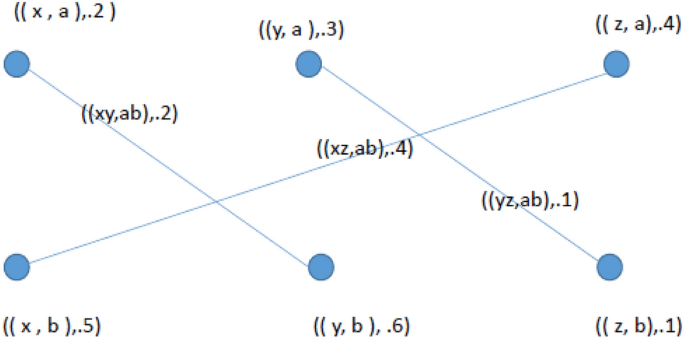
Consider any two plithogenic fuzzy graphs $P_{FG_{1}}=(P_{FV_{1}},Q_{FE_{1}})$ and $P_{FG_{2}}=(P_{FV_{2}},Q_{FE_{2}})$ of crisp graphs $G_{1}^{*}=(V_{1},E_{1})$ and $G_{2}^{*}=(V_{2},E_{2}),$ where $P_{FV_{1}}=\left( P_{1},\mu _{1},P_{\mu _{1}},\alpha _{1}{}_{_{Fdf}},\alpha _{1}{}_{_{FCf}}\right)$ & $Q_{FE_{1}}=$($Q_{1},\nu _{1},Q_{\nu _{1}},\beta _{1}{}_{_{Fdf}},\beta _{1}{}_{_{_{FCf}}})$ such that$(P_{1},Q_{1})$ is a graph with vertices $P_{1}=\{x,y,z\}$ and edges $Q_{1}=\{xy,yz,xz\},(\mu _{1},\nu _{1})$ be an attribute, $(P_{\mu _{1}},Q_{\nu _{1}})$ be a graph with vertices $P_{\mu _{1}}=\{a,b\}$ and edges $Q_{\nu _{1}}=\{ab\}.$ Also let $\alpha _{1}{}_{_{Fdf}}:P_{1}\times P_{\mu _{1}}\rightarrow [0,1]$ and $\alpha _{1}{}_{_{FCf}}:P_{\mu _{1}}\times P_{\mu _{1}}\rightarrow [0,1]$ be FDAFand FDCF for vertices defined as

also $\beta _{1}{}_{_{Fdf}}:Q_{1}\times Q_{\nu _{1}}\rightarrow [0,1]$ and $\beta _{1}{}_{_{_{FCf}}}:Q_{\nu _{1}}\times Q_{\nu _{1}}\rightarrow [0,1]$ be FDAFand FDCF for edges defined as

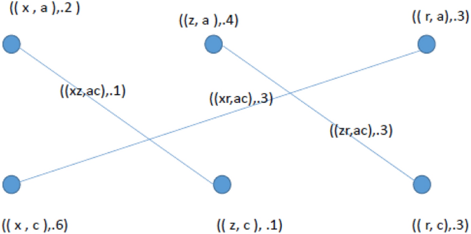
Then using the Definition 9, it is obvious that $P_{FG_{1}}$ is a plithogenic fuzzy graph as shown in Fig. 5. Also for plithogenic fuzzy graph $P_{FG_{2}};$ we have $P_{FV_{2}}=(P_{2}, \mu _{2},P_{\mu _{2}},\alpha _{2_{Fdf}},\alpha _{2}{}_{_{FCf}}) \& Q_{FE_{2}}=(Q_{2},\nu _{2},Q_{\nu _{2}},\beta _{2}{}_{_{Fdf}},\beta _{2}{}_{_{FCf}})$ such that $(P_{2},Q_{2})$ is a graph with vertices $P_{2}=\{x,z,r\}$ and edges $Q_{2}=\{xz,zr,xr\},(\mu _{2},\nu _{2})$ be an attribute$,(P_{\mu _{2}},Q_{\nu _{2}})$ is a graph with vertices $P_{\mu _{2}}=\{a,c\}$ and edges $Q_{\nu _{2}}=\{ac\}.$ Also let $\alpha _{2}{}_{_{Fdf}}:P_{2}\times P_{\mu _{2}}\rightarrow [0,1]$ and $\alpha _{2}{}_{_{FCf}}:P_{\mu _{2}}\times P_{\mu _{2}}\rightarrow [0,1]$ be FDAFand FDCF for vertices defined as

also $\beta _{2}{}_{_{Fdf}}:Q_{2}\times Q_{\nu _{2}}\rightarrow [0,1]$ and $\beta _{2}{}_{_{_{FCf}}}:Q_{\nu _{2}}\times Q_{\nu _{2}}\rightarrow [0,1]$ be FDAF and FDCF for edges defined as

Then using the Definition 9, it is obvious that $P_{FG_{2}}$ is a plithogenic fuzzy graph as shown in Fig. 6. Then their join is defined as $P_{FG_{1}+FG_{2}}=(P_{FV_{1}+FV_{2}},Q_{FE_{1}+FE_{2}})$ where $P_{FV_{1}+FV_{2}}=(P_{1}\cup P_{2},\mu _{1}\cup \mu _{2},P_{\mu _{1}\cup \mu _{2}},(\alpha _{1_{_{Fdf}}}+\alpha _{2_{_{Fdf}}}),(\alpha _{1_{FCf}}+\alpha _{2_{FCf}}))$ and $Q_{FE_{1}+FE_{2}}=(Q_{1}\cup Q_{2}\cup Q^{\prime },\nu _{1}\cup \nu _{2},Q_{\nu _{1}\cup \nu _{2}},(\beta _{1_{_{Fdf}}}+\beta _{2_{_{Fdf}}}),(\beta _{1_{FCf}}+\beta _{2_{FCf}})).$ Here we have $P_{1}\cup P_{2}=\{x,y,z,r\}$ ,$Q_{1}\cup Q_{2}=\{xy,yz,xz,zr,xr\}$ such that $(P_{1}\cup P_{2},Q_{1}\cup Q_{2})$ is a graph, $(\mu _{1}\cup \mu _{2},\nu _{1}\cup \nu _{2})$ is an attribute ,$P_{\mu _{1}\cup \mu _{2}}=\{a,b,c\}$ is range of attribute for vertices and $Q_{\nu _{1}\cup \nu _{2}}=\{ab,ac,bc\}$ is range of attribute for edges so that $(P_{\mu _{1}\cup \mu _{2}},Q_{\nu _{1}\cup \nu _{2}})$ is a graph. Here $(\alpha _{1_{Fdf}}+\alpha _{2_{Fdf}}):(P_{1}\cup P_{2})\times P_{\mu _{1}\cup \mu _{2}}\rightarrow [0,1]$ and $(\alpha _{1_{FCf}}+\alpha _{2_{FCf}}):P_{\mu _{1}\cup \mu _{2}}\times P_{\mu _{1}\cup \mu _{2}}\rightarrow [0,1]$ are FDAFand FDCF for vertices defined as in Table 13(i) and (ii).

also $(\beta _{1_{_{Fdf}}}+\beta _{2_{_{Fdf}}}):(Q_{1}\cup Q_{2}\cup Q^{\prime })\times Q_{\nu _{1}\cup \nu _{2}}\rightarrow [0,1]$ and $(\beta _{1_{FCf}}+\beta _{2_{FCf}}):Q_{\nu _{1}\cup \nu _{2}}\times Q_{\nu _{1}\cup \nu _{2}}\rightarrow [0,1]$ are FDAF and FDCF for edges and is defined as in Table 14(i) and (ii).

Using the Definition 11, it is obvious that $P_{FG_{1}+FG_{2}}$ is a plithogenic fuzzy graph as represented in Fig. 7a.

Table 9 FDAF and FDCF for vertices of $P_{FG_{1}}$

Table 10 FDAF and FDCF for edges of $P_{FG_{1}}$

Fig. 7

a Join of plithogenic fuzzy graphs P_FG1+FG2. b Join of two fuzzy graphs

Table 11 FDAF and FDCF for vertices of $P_{FG_{2}}$

Table 12 FDAF and FDCF for edges of $P_{FG_{2}}$

Fig. 8

Plithogenic fuzzy graph P_FG1

Table 13 (i) FDAF for vertices of $P_{FG_{1}+FG_{2}}$ and (ii) FDCF for vertices of $P_{FG_{1}+FG_{2}}$

Table 14 (i) FDAF for edges of $P_{FG_{1}+FG_{2}}$ and (ii) FDCF for edges of $P_{FG_{1}+FG_{2}}$

Fig. 9

A plithogenic fuzzy graph P_FG2

Remark 3

If we have only one attribute i.e if $a=b$ in plithogenic fuzzy graph $P_{FG_{1}}$and $a=c$ in plithogenic fuzzy graph $P_{FG_{2}}$ then join of plithogenic fuzzy graphs provided in Fig. 7a reduces to join of fuzzy graphs as shown in diagram Fig. 7b,

Fig. 10

Cartesian product of two plithogenic graphs

2.3 Cartesian product of plithogenic fuzzy graphs

Definition 12

Consider any two plithogenic graphs $P_{FG_{1}}=(P_{FV_{1}},Q_{FE_{1}})$ and $P_{FG_{2}}=(P_{FV_{2}},Q_{FE_{2}})$ as given in Definition 10 of crisp graphs $G_{1}^{*}=(V_{1},E_{1})$ and $G_{2}^{*}=(V_{2},E_{2}).$ We define their cartesian product as $P_{FG_{1}\times FG_{2}}=(P_{FM_{1}\times FM_{2}},P_{FN_{1}\times FN_{2}})$ where $P_{FM_{1}\times FM_{2}}=(M_{1}\times M_{2},\mu _{1}\times \mu _{2},\left( M_{\mu _{1}}\times M_{\mu _{2}}\right) ,\alpha _{1}{}_{_{Fdf}}\times \alpha _{2}{}_{_{Fdf}},\alpha _{1}{}_{_{FCf}}\times \alpha _{2}{}_{_{FCf}})$ is cartesian product of plithogenic sets for vertices; where $\left( M_{1}\times M_{2}\right) \subset \left( V_{1}\times V_{2}\right)$, $\mu _{1}\times \mu _{2}$ is an attribute, $\left( M_{\mu _{1}}\times M_{\mu _{2}}\right)$is the corresponding range of attribute values and $\alpha _{1}{}_{_{Fdf}}\times \alpha _{2}{}_{_{Fdf}}:\left( M_{1}\times M_{\mu _{1}}\right) \times \left( M_{2}\times M_{\mu _{2}}\right) \rightarrow \left[ 0,1\right]$ is the FDAF for vertices such that $(\alpha _{1_{_{Fdf}}}\times \alpha _{2_{_{Fdf}}})(\left( x_{1},x_{_{1\mu }}\right) ,\left( x_{2},x_{_{2\mu }}\right) )\in \left[ 0,1 \right] .$and is defined as (i)

$$\begin{aligned}&(\alpha _{1}{}_{_{Fdf}}\times \alpha _{2}{}_{_{Fdf}})(\left( x_{1},x_{_{1\mu }}\right) ,\left( x_{2},x_{_{2\mu }}\right) ) \\&=\min \{\alpha _{1}(x_{1},x_{_{1\mu }}),\alpha _{2_{Fdf}}(x_{2},x_{_{2\mu }})\} \end{aligned}$$

if $(\left( x_{1},x_{_{1\mu }}\right) ,\left( x_{2},x_{_{2\mu }}\right) )\in \left( M_{1}\times M_{\mu _{1}}\right) \times \left( M_{2}\times M_{\mu _{2}}\right) .$ Also $P_{_{FN_{1}\times FN_{2}}}=(N_{1}\times N_{2},\nu _{1}\times \nu _{2},\left( N_{\nu _{1}}\times N_{\nu _{2}}\right) ,(\beta _{1_{_{Fdf}}}\times \beta _{2_{_{Fdf}}}),(\beta _{1_{_{FCf}}}\times \beta _{2_{_{FCf}}}))$ is the cartesian product of plithogenic fuzzy sets for edges, where $\left( N_{1}\times N_{2}\right) \subset \left( E_{1}\times E_{2}\right)$, $\nu _{1}\times \nu _{2}$ is some attribute, $\left( N_{\nu _{1}}\times N_{\nu _{2}}\right)$ is the corresponding range of attribute values such that $(\beta _{1_{_{Fdf}}}\times \beta _{2_{_{Fdf}}}):(N_{1}\times N_{\nu _{1}})\times (N_{2}\times N_{\nu _{2}})\rightarrow \left[ 0,1\right]$ is the FDAF for edges defined as

(ii)

$$\begin{aligned}&(\beta _{1_{_{Fdf}}}\times \beta _{2_{_{Fdf}}})\left( \begin{array}{c} ((x,x_{_{\mu }}),(x_{2},x_{2_{\mu }})), \\ ((x,x_{_{\mu }}),(x_{2}^{\prime },x_{_{2\mu }}^{\prime })) \end{array} \right) \\= & {} \min \{\alpha _{1_{_{Fdf}}}(x,x_{_{\mu }}),\beta _{2_{_{Fdf}}}\left( (x_{2},x_{2_{\mu }}),(x_{2}^{\prime },x_{_{2\mu }}^{\prime })\right) \end{aligned}$$

for all $\left( ((x,x_{_{\mu }}),(x_{2},x_{2_{\mu }})),((x,x_{_{\mu }}),(x_{2}^{\prime },x_{_{2\mu }}^{\prime }))\right) \in (N_{1}\times N_{\nu _{1}})\times (N_{2}\times N_{\nu _{2}}).$

(iii)

$$\begin{aligned}&(\beta _{1_{_{Fdf}}}\times \beta _{2_{_{Fdf}}})\left( \begin{array}{c} ((x_{1},x_{1_{\mu }}),(x,x_{_{\mu }})), \\ ((x_{1}^{\prime },x_{1_{\mu }}^{\prime })),(x,x_{_{\mu }})) \end{array} \right) \\&=\min \{\beta _{1_{Fdf}}((x_{1},x_{1_{\mu }}),(x_{1}^{\prime },x_{1_{\mu }}^{\prime })),\alpha _{2_{Fdf}}(x,x_{_{\mu }})\} \end{aligned}$$

if $(((x_{1},x_{1_{\mu }}),(x,x_{_{\mu }})),((x_{1}^{\prime },x_{1_{\mu }}^{\prime })),(x,x_{_{\mu }})))\in (N_{1}\times N_{\nu _{1}})\times (N_{2}\times N_{\nu _{2}})$.

Also we have $\alpha _{1}{}_{_{FCf}}\times \alpha _{2}{}_{_{FCf}}:\left( M_{1\mu }\times M_{\mu _{1}}\right) \times \left( M_{\mu _{2}}\times M_{\mu _{2}}\right) \rightarrow \left[ 0,1\right]$ is FDCF for vertices ,such that $(\alpha _{1}{}_{_{FCf}}\times \alpha _{2}{}_{_{FCf}})(\left( x_{i\mu },x_{i_{\mu }}\right) ,(x_{i_{\mu }}^{\prime },x_{i_{\mu }}^{\prime }))=0;$ for all $(\left( x_{i\mu },x_{i_{\mu }}\right) ,(x_{i_{\mu }}^{\prime },x_{i_{\mu }}^{\prime }))\in \left( M_{\mu _{1}}\times M_{\mu _{1}}\right) \times \left( M_{\mu _{2}}\times M_{\mu _{2}}\right)$ and $(\alpha _{1}{}_{_{FCf}}\times \alpha _{2}{}_{_{FCf}})(\left( x_{i\mu },x_{j_{\mu }}\right) ,(x_{i_{\mu }}^{\prime },x_{j_{\mu }}^{\prime }))=(\alpha _{1}{}_{_{FCf}}\times \alpha _{2}{}_{_{FCf}})(\left( x_{j\mu },x_{i_{\mu }}\right) ,(x_{j_{\mu }}^{\prime },x_{i_{\mu }}^{\prime }))$ for all $(\left( x_{i\mu },x_{i_{\mu }}\right) ,(x_{i_{\mu }}^{\prime },x_{i_{\mu }}^{\prime }))\in \left( M_{\mu _{1}}\times M_{\mu _{1}}\right) \times \left( M_{\mu _{2}}\times M_{\mu _{2}}\right) .$ Also $(\beta _{1_{_{FCf}}}\times \beta _{2_{_{FCf}}}):\left( N_{\nu _{1}}\times N_{\nu _{2}}\right) \rightarrow \left[ 0,1\right]$ is FDCF for edges defined as

$$\begin{aligned} (\beta _{1_{_{FCf}}}\times \beta _{2_{_{FCf}}})\left( \begin{array}{c} ((x_{1\mu },x_{1\mu }),(x_{1\mu },x_{1\mu })), \\ ((x_{1\mu },x_{1\mu }),(,x_{1\mu },x_{1\mu })) \end{array} \right) =0 \end{aligned}$$

for all $\left( \begin{array}{c} ((x_{1\mu },x_{1\mu }),(x_{1\mu },x_{1\mu })), \\ ((x_{1\mu },x_{1\mu }),(,x_{1\mu },x_{1\mu })) \end{array} \right) \in \left( N_{\nu _{1}}\times N_{\nu _{2}}\right)$ and

$$\begin{aligned}&(\beta _{1_{_{FCf}}}\times \beta _{2_{_{FCf}}})\left( \begin{array}{c} ((x_{1\mu },x_{1\mu }),(x_{2\mu },x_{2\mu })), \\ ((x_{3\mu },x_{3\mu }),(,x_{4\mu },x_{4\mu })) \end{array} \right) \\&=(\beta _{1_{_{FCf}}}\times \beta _{2_{_{FCf}}})(\left( \begin{array}{c} (x_{3\mu },x_{3\mu }),(,x_{4\mu },x_{4\mu })), \\ ((x_{1\mu },x_{1\mu }),(x_{2\mu },x_{2\mu })) \end{array} \right) \end{aligned}$$

Then $P_{FG_{1}\times FG_{2}}=P_{FG_{1}\times FG_{2}}=(P_{FM_{1}\times FM_{2}},P_{FN_{1}\times FN_{2}})$ is a plithogenic fuzzy graph iff

$$\begin{aligned}&(\beta _{1_{_{Fdf}}}\times \beta _{2_{_{Fdf}}})(((x,a)(y,b)),((z,c),(r,d))) \nonumber \\&\le \min \left\{ \begin{array}{c} \left( (\alpha _{1_{_{Fdf}}}\times \alpha _{2_{_{Fdf}}})((x,a)(y,b))\right) , \\ \left( (\alpha _{1_{_{Fdf}}}\times \alpha _{2_{_{Fdf}}})((z,c),(r,d))\right) \end{array} \right\} \end{aligned}$$

(22)

for all $(((x,a)(y,b)),((z,c),(r,d)))\in (N_{1}\times N_{\nu _{1}})\times (N_{2}\times N_{\nu _{2}});$ also

$$\begin{aligned}&((\beta _{1_{FCf}}\times \beta _{2_{FCf}})(((a,b)(c,d)),((e,f),(g,h))) \nonumber \\&\le \min \left\{ \begin{array}{c} \left( (\alpha _{1_{_{_{FCf}}}}\times \alpha _{2_{FCf}})((a,b),(c,d)\right) , \\ \left( (\alpha _{1_{_{_{FCf}}}}\times \alpha _{2_{_{_{FCf}}}})((e,f),(g,h))\right) \end{array} \right\} \end{aligned}$$

(23)

for all $(((a,b)(c,d)),((e,f),(g,h))\in \left( N_{\nu _{1}}\times N_{\nu _{2}}\right) .$

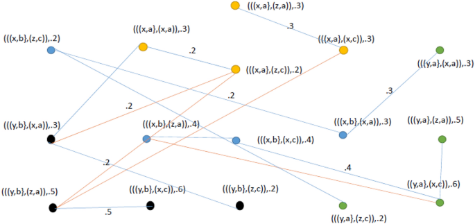
Example 4

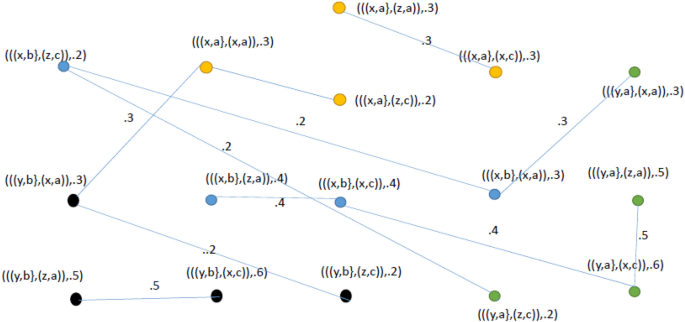
Let $G_{1}^{*}=(V_{1},E_{1})$ and $G_{2}^{*}=(V_{2},E_{2})$ be any two crisp graphs. Also suppose that $P_{FG_{1}}$and $P_{FG_{2}}$ be any two plithogenic fuzzy graphs such that $P_{FG_{1}}=(P_{FM_{1}},P_{FN_{1}}),$ where$P_{FM_{1}}=(M_{1},\mu _{1},M_{ \mu _{1}},\alpha _{1}{}_{_{Fdf}},\alpha _{1}{}_{_{FCf}}) \& \;P_{FN_{1}}=(N_{1},\nu _{1},N_{\nu _{1}},\beta _{1}{}_{_{Fdf}}, \beta _{1}{}_{_{_{FCf}}})$ and suppose that $M_{1}=\{x,y\} \subset V_{1}$ and $M_{\mu _{1}}=\{a,b\}$ is the corresponding range for some attribute. Also $N_{1}=\{xy\} \subset E_{1}$ and $\nu _{1}$ be some attribute for edges $N_{\nu _{1}}=\{ab\}$ be range of attribute. Then $\alpha _{1}{}_{_{Fdf}}:M_{1} \times M_{\mu _{1}}\rightarrow [0,1]$ and $\beta _{1}{}_{_{Fdf}}:$ $N_{1}\times N_{\nu _{1}}\rightarrow [0,1]$ is the FDAF for vertices $V_{1}$ and edges $E_{1}$ defined as and FDCF for vertices $V_{1}$ and edges $E_{1}$ is defined as Using the Definition 9, it is obvious that $P_{FG_{1}}$ is a plithogenic fuzzy graph as represented in Fig. 8. Also suppose that $M_{2}=\{x,z\} \subset V_{2}$ and $M_{\mu _{2}}=\{a,c\}$ is the corresponding range for some attribute. Also $N_{2}=\{xz\} \subset E_{1}$ and $\nu _{2}$ be some attribute for edges $N_{\nu _{2}}=\{ac\}$ be range of attribute. Then $\alpha _{2}{}_{_{Fdf}}:M_{2}\times M_{\mu _{2}}\rightarrow [0,1]$ and $\beta _{2}{}_{_{Fdf}}:$ $N_{2}\times N_{\nu _{2}}\rightarrow [0,1]$ is the FDAF for vertices $V_{2}$ and edges $E_{2}$ defined as

and FDCF for vertices $V_{2}$ and edges $E_{2}$ is defined as Using the Definition 9, it is obvious that $P_{FG_{2}}$ is a plithogenic fuzzy graph as represented in Fig. 9. Hence Using the Definition 12, the FDAF of cartesian product for vertices $\left( \alpha _{1}\times \alpha _{2}\right) _{_{Fdf}}:\left( M_{1}\times M_{1\mu }\right) \times \left( M_{2}\times M_{\mu _{2}}\right) \rightarrow \left[ 0,1\right]$ is given by (i) $\left( \alpha _{1}\times \alpha _{2}\right) _{_{Fdf}}(\left( x_{1},x_{_{1\mu }}\right) ,\left( x_{2},x_{_{2\mu }}\right) )=\min \{ \alpha _{1}(x_{1},x_{_{1\mu }}),\alpha _{2_{Fdf}}(x_{2},x_{_{2\mu }})\}$if $(\left( x_{1},x_{_{1\mu }}\right) ,\left( x_{2},x_{_{2\mu }}\right) )\in \left( M_{1}\times M_{1\mu }\right) \times \left( M_{2}\times M_{\mu _{2}}\right) .$ Here $M_{1}\times M_{\mu _{1}}=\{(x,a),(x,b),(y,a),(y,b)\}$ and $M_{2}\times M_{\mu _{2}}=\{(x,a),(x,c),(z,a),(z,c)\}.$ Hence

1. $(\alpha _{1}{}_{_{Fdf}}\times \alpha _{2}{}_{_{Fdf}})(\left( x,a\right) ,\left( x,c\right) )=\min \{ \alpha _{1}(x,a),\alpha _{2_{Fdf}}(x,c)\}=0.3,$

2. $(\alpha _{1}{}_{_{Fdf}}\times \alpha _{2}{}_{_{Fdf}})(\left( x,b\right) ,\left( x,c\right) )=\min \{ \alpha _{1}(x,b),\alpha _{2_{Fdf}}(x,c)\}=0.4,$

3. $(\alpha _{1}{}_{_{Fdf}}\times \alpha _{2}{}_{_{Fdf}})(\left( x,b\right) ,\left( z,c\right) )=\min \{ \alpha _{1}(x,a),\alpha _{2_{Fdf}}(x,c)\}=0.2$

4. $(\alpha _{1}{}_{_{Fdf}}\times \alpha _{2}{}_{_{Fdf}})(\left( x,b\right) ,\left( z,a\right) )=\min \{ \alpha _{1}(x,b),\alpha _{2_{Fdf}}(z,a)\}=0.4$

5. $(\alpha _{1}{}_{_{Fdf}}\times \alpha _{2}{}_{_{Fdf}})(\left( y,a\right) ,\left( z,a\right) )=\min \{ \alpha _{1}(y,a),\alpha _{2_{Fdf}}(z,a)\}=0.5$ and so on.

Similarly for edges we have

6.

$$\begin{aligned}&\left( \beta _{1}\times \beta _{2}\right) _{Fdf}\left( ((x,a),(x,c)),((x,a),(z,c))\right) \\= & {} \min \{\alpha _{1}(x,a),\beta _{2Fdf}\left( (x,c),(z,c)\right) =0.2 \end{aligned}$$

7.

$$\begin{aligned}&\left( \beta _{1}\times \beta _{2}\right) _{Fdf}\left( ((x,a),(z,a)),((x,a),(z,c))\right) \\= & {} \min \{\alpha _{1}(x,a),\beta _{2Fdf}\left( (z,a),(z,c)\right) =0.2 \end{aligned}$$

8.

$$\begin{aligned}&\left( \beta _{1}\times \beta _{2}\right) _{Fdf}\left( (x,b),(x,a)),((y,b)),(x,a))\right) \\= & {} \min (\beta _{1_{Fdf}}\left( (x,b),(y,b)\right) ,\alpha _{2_{Fdf}}(x,a))=0.4 \end{aligned}$$

9-

$$\begin{aligned}&\left( \beta _{1}\times \beta _{2}\right) _{Fdf}\left( (y,a),(x,a)),((y,b)),(x,a))\right) \\= & {} \min (\beta _{1_{Fdf}}\left( (y,a),(y,b)\right) ,\alpha _{2_{Fdf}}(x,a))=0.2 \end{aligned}$$

and so on. Hence $P_{FG_{1}\times FG_{2}}$ is a plithogenic fuzzy graph as shown in Fig. 10.

Table 15 FDAF and FDCF for vertices of $P_{FG_{1}}$

Table 16 FDAF and FDCF for edges of $P_{FG_{1}}$

Fig. 11

Composition of two plithogenic fuzzy graphs

Table 17 FDAF and FDCF for vertices of $P_{FG_{2}}$

Table 18 FDAF and FDCF for edges of $P_{FG_{2}}$

Fig. 12

a A plithogenic graph showing effects of diffrent CoVs. b A fuzzy graph showing effects of different CoVs. c An intuitionistic fuzzy graph showing effects of different CoVs. d A nutrosophic graph showing effects of different CoVs

Fig. 13

a Plithogenic graph showing spreading of COVID-19. b Fuzzy graph showing spreading of COVID-19. c A intuitionistic fuzzy graph showing spreading of COVID-19. d A neutrosophic graph showing spreading of COVID-19

2.4 Composition of plithogenic fuzzy graphs

Consider the Example 4 then the composition of plithogenic fuzzy graphs $P_{FG_{1}}$ and $P_{FG_{2}}$ is represented in Fig. 11.

3 Results and analysis

3.1 Experimental results (global spread of COVID-19)

Coronaviruses (CoV) are a large family of viruses that cause illnesses ranging from the common cold to more severe diseases such as Middle East Respiratory Syndrome (MERS-CoV) and Severe Acute Respiratory Syndrome (SARS-CoV). A novel coronavirus (nCoV) is a new strain that has not been previously identified in humans. It has been discussed and tried to verify how these viruses affected human beings during their outbreaks. We are usig the database taken from the following source https://coronavirus.jhu.edu/map.html.

Example 5

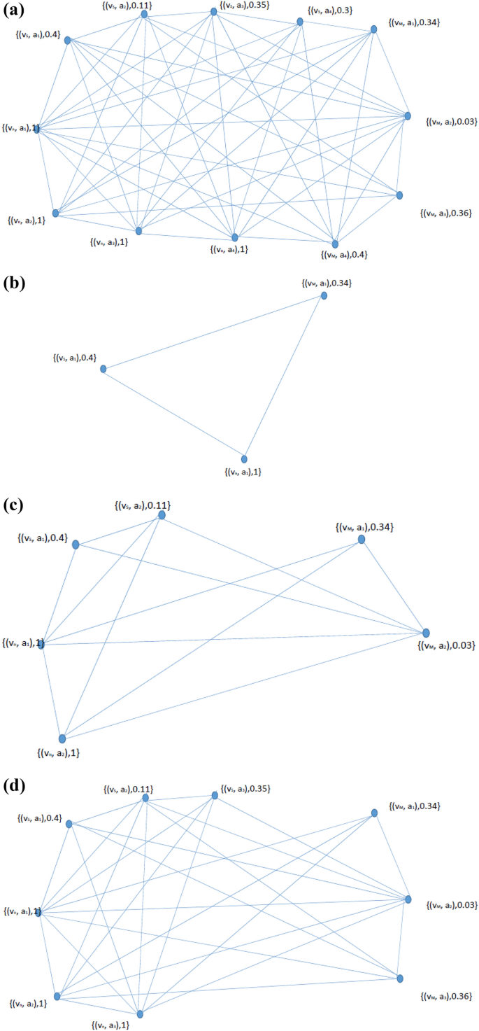
We are discussing how these viruses affected the world at different times for different durations. Let $G^{*}=(V,E)$ be a crisp graph where V is the set of different types of fatalic viruses and $P\subset V$ be types of coronavirus. Let us denote these types (1) $V_{S}=$ SARS-CoV; (2) $V_{M}=$ MERS-CoV; $V_{n}=$COVID-19. Let $\chi =$ attribute which denote the effects of these coronaviruses in different years for different durations on the whole world and range of this attribute is $a_{1}=$ number of countries effected, $a_{2}=$ number of people effected, $a_{3}=$ number of casualities, $a_{4}=$ duration. Then we have $P=$ $\{V_{S},V_{M},V_{n}\}$ and range of attribute for vertices $P_{\chi }=\{a_{1},a_{2},a_{3},a_{4}\}$. Also $Q=\{V_{S}V_{M},V_{M}V_{n},V_{S}V_{n}\}\subseteq E\subseteq V\times V$ and $\nu$ be some attribute for edges, such that ( $P_{\chi },Q_{\nu })$ forms a graph. Then we have

$P_{\chi }\backslash P$	$V_{S}$	$V_{M}$	$V_{n}$
$a_{1}$	32	27	79
$a_{2}$	8, 096	2, 260	75, 571
$a_{3}$	774	803	2239
$a_{4}$	2002–2003	2018	Dec 2019–2020

Let the FDAF for vertices be $\alpha _{Fdf}:P\times P_{\chi }\rightarrow \left[ 0,1\right]$ defined by $\alpha _{Fdf}(\frac{V_{i}}{Vm},\frac{aj}{ a_{m}});$ where $i=$ S, M, n ; $m=$ largest number with maximum effect and $j=1,2,3.$ where as for $a_{4}$ we have membership function as duration for which these coronavirses proved to be more fatalic. So we have FDAF and FDCF for vertices as in Table 19(i) and (ii).

Also FDAF and FDCF for edges

$$\begin{aligned} \beta _{Fdf}:Q\times Q_{\nu }\rightarrow \left[ 0,1\right] \end{aligned}$$

and

$$\begin{aligned} \beta _{Fdf}:Q\times Q_{\nu }\rightarrow \left[ 0,1\right] \end{aligned}$$

which is defined as main reason for spreading of these viruses i.e.for $V_{S}$ through bats, $V_{M}$ through bats and animal flesh and $V_{n}$ through all the previous reasons including human to human interaction, also low immunity, see Table 20(i) and (ii).

Hence $P_{FG}=(P_{FV},Q_{FE})$ is plithogenic graph as shown in Fig. 12a.

Table 19 (i) FDAF for vertices of $P_{FG}$ and (ii) FDCF for vertices of $P_{FG}$

Table 20 (i): FDAF for edges of $P_{FG}$ and (ii) FDCF for edges of $P_{FG}$

Example 6

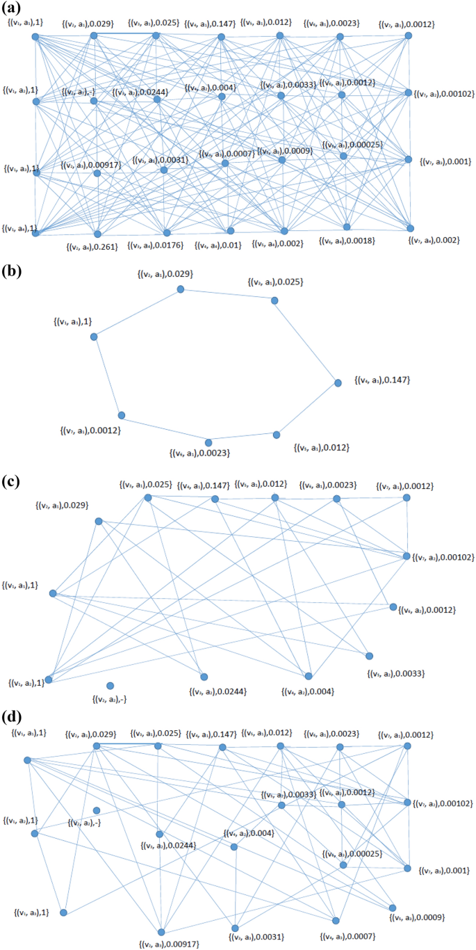
Let us consider the case of the novel Coronavirus(COVID-19), and we want to measure its overall effect on the whole world. There are a lot of factors to discuss, but here we discuss some of them. Let $G^{*}=(V,E)$ be a crisp graph where V is the set of different countries effected by new Coronavirus COVID-19 and let $P(\subset V)$ consisting of highly effected countries having casualities. Let us denote countries $v_{1}=$ China, $v_{2}=$ Iran, $v_{3}=$ Italy, $v_{4}=$ South Korea, $v_{5}=$ Japan, $v_{6}=$ France, $v_{7}=$ United State. $P=\left\{ v_{1},v_{2},v_{3},v_{4},v_{5},v_{6},v_{7}\right\} .$ Let $\mu =$ attribute is Coronavirus COVID-19 and range of attribute is $a=$ confirmed cases having Coronavirus COVID-19, $b=$ serious, critical cases having Coronavirus COVID-19, $c=$recovered cases having Coronavirus COVID-19, $d=$ casualities with Coronavirus COVID-19. Then we have

$P\mu \backslash P$	$v_{1}$	$v_{2}$	$v_{3}$	$v_{4}$	$v_{5}$	$v_{6}$	$v_{7}$
$a_{1}$	80, 152	2, 336	2, 036	5, 186	989	191	103
$a_{2}$	6, 806	−	166	27	23	8	7
$a_{3}$	47, 396	435	149	34	43	12	9
$a_{4}$	2, 945	77	52	28	12	3	6

then FDAF for vertices $\alpha _{Fdf}:P\times P_{\mu }\rightarrow \left[ 0,1\right]$ is defined by $\alpha _{Fdf}(\frac{v_{i}}{v_{m}},\frac{a_{i}}{ a_{m}})\in \left[ 0,1\right]$ where $v_{m}=$ country with maximum cases and $a_{m}=$ maximum number in any attribute. Then for vertices FDAF and FDCF is given by Tables 21(i) and (ii).

Let FDAF for edges be

$$\begin{aligned} \beta _{Fdf}:Q\times Q_{\nu }\rightarrow \left[ 0,1\right] \end{aligned}$$

defined as in Table 22(i) and (ii).

which is defined as main reason for spreading i.e. means of travelling (through flights or roads) between these countries , trade,tourism, lack of vaccination, then for all $((v_{i},a_{k}),(v_{j},a_{l}))\in Q\times Q;$ we have

$$\begin{aligned} \beta _{Fdf}((v_{i},a_{k}),(v_{j},a_{l}))\le \min \left( \begin{array}{c} \alpha _{Fdf}(v_{i},a_{k}), \\ \alpha _{Fdf}(v_{j},a_{l}) \end{array} \right) \end{aligned}$$

where $i\ne j;i,j=1,2,3,4,5,6,7.$ and $k\ne l;k,l=1,2,3,4.$ Also $\alpha _{FCf}(a_{i},a_{i})=0$ and $\alpha _{FCf}(a_{i},a_{j})=\alpha _{FCf}(a_{j},a_{i}).$ Hence $P_{FG}$ is plithogenic graph as shown in Fig. 13,

Table 21 (i) FDAF for vertices of $P_{FG}$. (ii) FDCF for vertices of $P_{FG}$

Table 22 (i):FDAF for edges of $P_{FG}$. (ii) FDCF for edges of $P_{FG}$

3.2 Analysis (results)

Following results have been derived from the mathematical study:

• 1. We Provided the mathematical existence of Plithogenic’ graphs through examples that generalize fuzzy, intuitionistic, and neutrosophic graphs.

• 2. We established different binary opertions of Plithogenic graphs for practical use in real-life applications.

• 3. COVID-19 was found much dangerous than (MERS-CoV) and (SARS-CoV).

• 4. Figure 11 shows that COVID-19 seems to be Chimera of two viruses.

• 5. As the SARS-CoV and MERS-CoV outbreaks were controlled, there are greater chances to overcome the current pandemic of COVID-19.

• 6. The global spread of COVID-19 is associated with traveling, as the edges of Fig. 12a suggest.

• 7. If the value of an edge is 0, it means that there is no traveling between two particular countries, so the spread of COVID-19 is 0.

• 8. This model suggests that all the countries should stop all types of traveling/movement across the borders and inside the country.

• 9. We predict if precautionary measures have not been taken, then there is a chance of severe outbreaks in the future.

• 10. The performance metrics of our proposed mathematical model indicated that the COVID-19 is zoonotic, and the human transmission is very fast in the case of frequent travel.

4 Comparison analysis

In this paper, we extend the plithogenic sets to plithogenic graphs. As we see that in plithogenic graphs. we have $P_{G}=(P_{M},P_{N})$ ,where $P_{M}=(M,\mu ,M_{\mu },\alpha _{df},\alpha _{Cf})$ is plithogenic set $P_{S}$ for vertices; where $M\subset V$, $\mu$ is an attribute, $M_{\mu }$ is the corresponding range of attribute values such that $\alpha _{df}:M\times M_{\mu }\rightarrow \left[ 0,1\right] ^{s}$ is the DAF for vertices defined as $\alpha _{df}(v_{1}$, $\mu _{1})\in \left[ 0,1\right] ^{s}.$and $\alpha _{Cf}:M_{\mu }\times M_{\mu }\rightarrow \left[ 0,1\right] ^{t}$is DCF for vertices. Also $P_{N}=(N,\nu ,N_{\nu },\beta _{df},\beta _{Cf})$ is plithogenic set for edges, where $N\subset E$ , $\nu$ is the some attribute, $N_{\nu }$ is the corresponding range of attribute values for edges such that $\beta _{df}:N\times N_{\mu }\rightarrow \left[ 0,1\right] ^{s}$is the DAF for edges and $\beta _{Cf}:N_{\nu }\times N_{\nu }\rightarrow \left[ 0,1\right] ^{t}$ is DCF for edges. Then $P_{G}$ is plithogenic graph iff for all $(v_{1},\mu _{1})$& $(v_{2},\mu _{2})\in M\times M_{\mu }$; $\beta _{_{df}}((v_{1},\mu _{1})(v_{2},\mu _{2}))\le \alpha _{_{df}}((v_{1},\mu _{1})\wedge \alpha _{_{df}}(v_{2},\mu _{2}))$. Here $s,t\in \{1,2,3\}.$ If we take the set of edges as null set then our model reduces to plithogenic set $P_{S}=(P,\chi ,P_{\chi },p_{df},p_{_{CF}})$ where $\chi$ is an appurtenance or attribute, $P_{\chi }$ is corresponding range of attribute’s value, $p_{df}:P\times P_{\chi }\rightarrow [0,1]^{s}$ is the degree of appurtenance function and $p_{_{CF}}:P_{\chi }\times P_{\chi }\rightarrow [0,1]^{t}$ is the corresponding degree of contradiction function. Here $s,t\in \{1,2,3\}.$

1. Consider the Example 5. (a) if we have only one attribute i.e., $a_{1}=$ number of countries effected then plithogenic fuzzy graph provided in Fig. 12a reduces to fuzzy graph as shown in Fig. 12b. (b) If we have two attributes suppose $a_{1}=$ number of countries effected and $a_{2}=$number of people effected then plithogenic fuzzy graph provided in Fig. 12a reduces to intuitionistic fuzzy graph as shown in Fig. 12c (c) If we take three attributes say $a_{1}=$ number of countries effected and $a_{2}=$number of people effected $a_{3}=$ number of casualties then plithogenic fuzzy graph provided in Fig. 12a reduces to neutrosophic graph as shown in Fig. 12d. 2. Consider the Example 6. (a) If we take only one attribute say $a_{1}=$confirmed cases having COVID-19 then plithogenic fuzzy graph provided Fig. 13a reduces to fuzzy graph as shown in Fig. 13b. (b) If we have two attributes suppose $a_{1}=$ confirmed cases with COVID-19 and $a_{2}=$ serious, critical cases having COVID-19 then plithogenic fuzzy graph provided in Fig. 13a reduces to intuitionistic fuzzy graph as shown in Fig. 13c. (c) If we consider three attributes i.e. $a_{1}=$confirmed cases with COVID-19, $a_{2}=$ critical cases having Coronavirus COVID-19, $a_{3}=$ recovered cases of COVID-19, then plithogenic fuzzy graph provided in Fig. 13a reduces to neutrosophic graph as shown in Fig. 13d. Thus our model of plithogenic graph is better than already existing graphs as it can capture more information.

5 Conclusions

Initially, the virus was zoonotic in origin, and then it was spread by human interactions (person to person). Our model verified that its spread across the borders was mainly due to travelers. To control the COVID-19, it is strongly recommended to go for self-isolation to break the chain by making the edges of Plithogenic graphs equal to 0. The animals or their food which is thought to be the source of this virus, should be banned in the markets, and personal hygiene should be maintained to reduce the spread. This mathematical model can be applied to assess the spread of COVID-19 in any region of the world.

6 Future work

In the future, we aim to make more different types of graphs in the circumstances of plithogenic theory by taking more attributes and other approaches. This model has been initially applied on database taken from the following source https://coronavirus.jhu.edu/map.html. We are aiming to use this model on some other database in the future.

References

Abdel-Basset M, El-hoseny M, Gamal A, Smarandache F (2019) A novel model for evaluation hospital medical care systems based on plithogenic sets. Artif Intell Med 100:1–8. https://doi.org/10.1016/j.artmed.2019.101710
Abdel-Basset M, Mohamed R (2019) A novel plithogenic topsis-critic model for sustainable supply chain risk management. J Clean Prod 24:7119587. https://doi.org/10.1016/j.jclepro.2019.119586
Abdel-Basset M, Mohamed R, Zaied ANH, Smarandache F (2019) A hybrid plithogenic decision-making approach with quality function deployment for selecting supply chain sustainability metrics. Symmetry 11:903. https://doi.org/10.3390/sym11070903
Ahmad T, Khan M, Haroon Musa TH, Nasir S, Hui J, Bonilla-Aldana DK, Rodriguez-Morales AJ (2020) COVID-19: zoonotic aspects. Travel Med Infect Dis 36:101607. https://doi.org/10.1016/j.tmaid.2020.101607
Akram M (2012) Interval-valued fuzzy line graphs. Neural Comput Appl 21:145–150. https://doi.org/10.1007/s00521-011-0733-0
Akram M, Dudek WA (2011) Interval-valued fuzzy graphs. Comput Math Appl 61:289–299. https://doi.org/10.5391/IJFIS.2020.20.4.316
Akram M, Alshehri NO, Dudek WA (2013) Certain types of interval-valued fuzzy graphs. J Appl Math 2013:857070. https://doi.org/10.1155/2013/857070
Atanassov KT (1986) Intuitionistic fuzzy sets. Fuzzy Sets Syst 20:87–96. https://doi.org/10.1016/S0165-0114(86)80034-3
Atanassov KT (1995) On intuitionistic fuzzy graphs and intuitionistic fuzzy relations. In: Proceedings of the VI IFSA world cong, Sao Paulo, Brazil, vol 1, p 551–554
Bhattacharya P (1987) Some remarks on fuzzy graphs. Pattern Recognit Lett 6:297–302. https://doi.org/10.1016/0167-8655(87)90012-2
Gayen S, Smarandache F, Jha S, Singh MK, Broumi S, and Kumar R (2019) Chapter 8: Introduction to plithogenic subgroup. In: Neutrosophic graph theory and algorithm. p 209–233. IGI-Global, Pennsylvania
Gayen S, Smarandache F, Jha S, Singh MK, Broumi S, Kumar R (2020) Introduction to plithogenic hypersoft subgroup. Neutrosophic Sets nd Syst 33:208–233
Gulistan M, Yaqoob N, Rashid Z, Smarandache F, Wahab HA (2018) A study on neutrosophic cubic graphs with real life applications in industries. Symmetry 10:203. https://doi.org/10.3390/sym10060203
Gulistan M, Ali M, Azhar M, Rho S, Kadry S (2019) Novel neutrosophic cubic graphs structures with application in decision making problems. IEEE Access 7:94757–94778. https://doi.org/10.1109/ACCESS.2019.2925040
Huang L, Yu Hu, Kishore PK (2019) A study of regular and irregular neutrosophic graphs with real life applications. Mathematics 7:551. https://doi.org/10.3390/math7060551
Jun YB, Kim CS, Kang MS (2010) Cubic sub-algebra and ideals of BCK/BCI-algebra. Far East J Math Sci 44:239–250
Jun YB, Lee KJ, Kang MS (2011) Cubic structures applied to ideals of BCI-algebra. Comput Math Appl 62:3334–3342. https://doi.org/10.1016/j.camwa.2011.08.042
Jun YB, Kim CS, Yang KO (2012) Cubic sets. Ann Fuzzy Math Inf 4:83–98
Jun YB, Smarandache F, Kim CS (2017a) Neutrosophic cubic sets. New Math Nat Comput 13:41–54. https://doi.org/10.1142/S1793005717500041
Jun YB, Smarandache F, Kim CS (2017b) P-union and P-intersection of neutrosophic cubic sets. Versita 25:99–115. https://doi.org/10.1515/auom-2017-0009
Kandasamy WBV, Ilanthenral K, Smarandache F (2015) Neutrosophic graphs: a new dimension to graph theory. Bruxelles, Europa NovaASBL
Kauffman A (1973) Introduction a la Theorie des Sous-Emsembles Flous; Masson: Issy-les-Moulineaux, French,vol 1
Khan FM, Ahmad T, Gulistan M, Chammam W, Khan M, Hui J (2021) Epidemiology of coronaviruses, genetics, vaccines, and scenario of current pandemic of coronavirus disease 2019 (COVID-19): a fuzzy set approach. Hum Vacc Immunother 17:1296–1303. https://doi.org/10.1080/21645515.2020.1798697
Rana S, Qayyum M, Saeed M, Smarandache F (2019) Plithogenic fuzzy whole hypersoft set: construction of operators and their application in frequency matrix multi attribute decision making technique. Neutrosophic Sets Syst 28:34–50
Rashid S, Yaqoob N, Akram M, Gulistan M (2018) Cubic graphs with application. Int J Anal Appl 16:733–750. https://doi.org/10.28924/2291-8639
Rosenfeld A (1975) Fuzzy graphs, fuzzy sets and their applications. Academic Press, New York, pp 77–95
Rodriguez-Morales AJ, Cardona-Ospina JA, Gutiérrez-Ocampo E, Villamizar-Peña R, Holguin-Rivera Y, Escalera-Antezana JP, Alvarado-Arnez LE, Bonilla-Aldana DK, Franco-Paredes C, Henao-Martinez AF, Paniz-Mondolfi A, Lagos-Grisales GJ, Ramírez-Vallejo E, Suárez JA, Zambrano LI, Villamil-Gómez WE, Balbin-Ramon GJ, Rabaan AA, Harapan H, Dhama K, Nishiura H, Kataoka H, Ahmad T, Sah R (2020) Clinical, laboratory and imaging features of COVID-19: a systematic review and meta-analysis. Travel Med Infect Dis 34:101623. https://doi.org/10.1016/j.tmaid.2020.101623
Shannon A, Atanassov KT (1994) A first step to a theory of the Intuitionistic fuzzy graphs. In: Proceedings of the1st workshop on fuzzy based expert systems, Sofia, Bulgaria, p 26–29, 59–61
Smarandache F (1999) A unifying field in logics. Neutrosophic logic. Neutrosophy, neutrosophic set, neutrosophic probability. American Research Press, Rehoboth
Smarandache F (2005) Neutrosophic set—a generalization of the intuitionistic fuzzy set. J Defen Resour Manag 1:107–116
Smarandache F (2017) Plithogeny, Plithogenic set, Logic, Probability, and Statistic. Brussels, Belgium. arXiv:1808.03948
Smarandache F (2018a) Plithogenic set, an extension of crisp, fuzzy, intuitionistic fuzzy, and neutrosophic sets-revisited. Neutrosophic Sets Syst 21:153–166
Smarandache F (2018b) Extension of soft set to hypersoft set, and then to plithogenic hypersoft set. Octogon Math Mag 27:413–418
Smarandache F (2018c) Physical plithogenic set. In: APS annual gaseous electronics meeting abstracts, p LW1-118
Smarandache F (2018d) Aggregation plithogenic operators in physical fields. In: 71st annual meeting of the APS division of fluid dynamics. Bulletin of the American Physical Society, vol 63. https://meetings.aps.org/Meeting/DFD18/ Event/334150
Smarandache F, Broumi S (2018) Neutrosophic graph theory and algorithms, vol 8. Pennsylvania, IGI Global, pp 213–259
Yaqoob N, Gulistan M, Kadry S, Wahab HA (2019) Complex intuitionistic fuzzy graphs with application in cellular network provider companies. Mathematics 7:35. https://doi.org/10.3390/math7010035
World Health Organization (2020) Naming the coronavirus disease (COVID-19) and the virus that causes it. https://www.who.int/emergencies/diseases/novel-coronavirus-2019/technical-guidance/naming-the-coronavirus-disease-(covid-2019)-and-the-virus-that-causes-it. Accessed 01 Apr 2020
Wang H, Smarandache F, Zhang YQ, Sunderraman R (2005) Interval neutrosophic sets and logic: theory and applications in computing; Hexis: phoenix, AZ, USA. http://fs.unm.edu/INSL.pdf
Zadeh LA (1996) Fuzzy sets, fuzzy logic, and fuzzy systems: In: Advances in fuzzy systems—applications and theory. World Scientific 6. https://www.worldscientific.com/worldscibooks /10.1142/2895
Zadeh LA (1975) The concept of a linguistics variable and its application to approximate reasoning-I. Inf Sci 8:301–357. https://doi.org/10.1016/0020-0255(75)90046-8
Acknowledgements
Authors are highly thankful to the Editor and anonymous reviewers for their valuable suggestions to bring this paper in the present form.
Author information
Authors and Affiliations
Corresponding author
Ethics declarations
Conflict of interest
Authors declare that there is no conflict of interest.
Ethical approval
The present article does not contain any studies with human participants or animals performed by any of the authors.
Additional information
Publisher's Note
Springer Nature remains neutral with regard to jurisdictional claims in published maps and institutional affiliations.
Rights and permissions
About this article
Cite this article
Sultana, F., Gulistan, M., Ali, M. et al. A study of plithogenic graphs: applications in spreading coronavirus disease (COVID-19) globally. J Ambient Intell Human Comput 14, 13139–13159 (2023). https://doi.org/10.1007/s12652-022-03772-6
Received:
Accepted:
Published:
Issue Date:
DOI: https://doi.org/10.1007/s12652-022-03772-6