
Abstract
Multi-way data arises in many applications such as electroencephalography classification, face recognition, text mining and hyperspectral data analysis. Tensor decomposition has been commonly used to find the hidden factors and elicit the intrinsic structures of the multi-way data. This paper considers sparse nonnegative Tucker decomposition (NTD), which is to decompose a given tensor into the product of a core tensor and several factor matrices with sparsity and nonnegativity constraints. An alternating proximal gradient method is applied to solve the problem. The algorithm is then modified to sparse NTD with missing values. Per-iteration cost of the algorithm is estimated scalable about the data size, and global convergence is established under fairly loose conditions. Numerical experiments on both synthetic and real world data demonstrate its superiority over a few state-of-the-art methods for (sparse) NTD from partial and/or full observations. The MATLAB code along with demos are accessible from the author’s homepage.


Notes
There appears no exact definition of “large-scale”. The concept can involve with the development of the computing power. Here, we roughly mean there are over millions of variables or data values.
Here, by scalability, we mean the cost is no greater than \(s\cdot \log (s)\) if the data size is \(s\).
Since the problem is non-convex, we only get convergence to a stationary point, and different starting points can produce different limit points.
For the case that \(\varvec{\mathcal {C}}\) is also Gaussian randomly generated, the performance of APG and HALS is similar.
The code of HONMF is implemented for NTD with missing value. Its running time would be reduced if it were implemented separately for the NTD. However, we observe that HONMF converges much slower than our algorithm.
The mode-\(n\) ranks of \(\varvec{\mathcal {M}}\) are 24, 14, and 13 for \(n=1,2,3\), respectively. Larger size is used to improve the data fitting.
Sometimes, APG is also trapped at some local solution. We run the three algorithms on the Swimmer dataset to maximum 30 seconds. If the relative error is below \(10^{-3}\), we regard the algorithm reaches a global solution. Among 20 independent runs, APG, HONMF, and HALS reach a global solution 11, 0, and 5 times, respectively. We also test the three algorithms with smaller rank (24,18,17), in which case APG, HONMF, and HALS reach a global solution 16, 0, and 4 times respectively among 20 independent runs.
Fig. 4 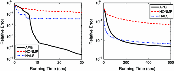
Convergence behavior of APG, HONMF, and HALS on Swimmer dataset (left) and a brain MRI image (right)
In the implementation of HALS, all factor matrices are re-scaled such that each column has unit length after each iteration. The re-scaling is necessary for efficient update of the core tensor and does not change the objective value of (5) if all sparsity paramenters are zero. However, it will change the objective if some of \(\lambda _c,\lambda _1,\ldots ,\lambda _N\) are positive.
Although HONMF converges very slowly, it is the only one we can find that is also coded for sparse nonnegative Tucker decomposition with missing values.
We permute the columns of the factor matrices and do permutations to the core tensor accordingly.
Fig. 6 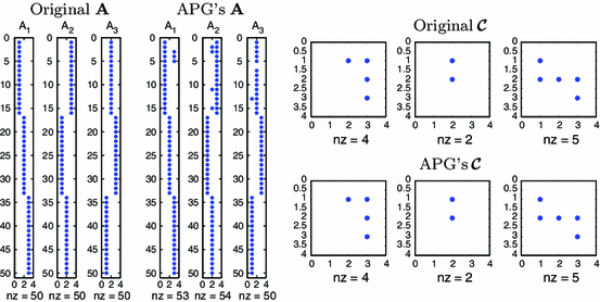
Sparsity pattern of the orginal \(\varvec{\mathcal {C}}\) and \(\mathbf {A}\) and those given by APG method
In tensor-matrix multiplications, unfolding and folding a tensor both happens, and they can take about a half of time in the whole process of tensor-matrix multiplication. The readers can refer to [30] for issues about the cost of tensor unfolding and permutation.


References
Allen, G.I.: Sparse higher-order principal components analysis. In: International conference on artificial intelligence and statistics (AISTATS), pp 27–36 (2012)
Bader, B.W., Kolda, T.G., et al.: Matlab tensor toolbox version 2.5 (2012). http://www.sandia.gov/~tgkolda/TensorToolbox
Beck, A., Teboulle, M.: A fast iterative shrinkage-thresholding algorithm for linear inverse problems. SIAM J. Imaging Sci. 2, 183–202 (2009)
Bolte, J., Daniilidis, A., Lewis, A.: The Lojasiewicz inequality for nonsmooth subanalytic functions with applications to subgradient dynamical systems. SIAM J. Optim. 17, 1205–1223 (2007)
Carroll, J.D., Chang, J.J.: Analysis of individual differences in multidimensional scaling via an N-way generalization of “Eckart-Young” decomposition. Psychometrika 35, 283–319 (1970)
Cichocki, A., Mandic, D., Phan, A.H., Caiafa, C., Zhou, G., Zhao, Q., De Lathauwer, L.: Tensor decompositions for signal processing applications: from two-way to multiway component analysis. arXiv:1403.4462 (2014)
Cichocki, A., Zdunek, R., Phan, A.H., Amari, S.: Nonnegative Matrix and Tensor Factorizations: Applications to Exploratory Multi-way Data Analysis and Blind Source Separation. Wiley, UK (2009)
Cong, F., Phan, A.H., Zhao, Q., Wu, Q., Ristaniemi, T., Cichocki, A.: Feature extraction by nonnegative tucker decomposition from EEG data including testing and training observations. Neural Inf. Process. 3, 166–173 (2012)
De Lathauwer, L., De Moor, B., Vandewalle, J.: On the best rank-1 and rank-\((r_1, r_2,\ldots, r_n)\) approximation of higher-order tensors. SIAM J. Matrix Anal. Appl. 21, 1324–1342 (2000)
Ding, C., Li, T., Jordan, M.: Convex and semi-nonnegative matrix factorizations. Pattern Anal. Mach. Intell. IEEE Trans. 32, 45–55 (2010)
Donoho D., Stodden, V.: When does non-negative matrix factorization give a correct decomposition into parts. Adv. Neural Inf. Process. Syst. 16 (2003)
Friedlander, M.P., Hatz, K.: Computing non-negative tensor factorizations. Optim. Methods Softw. 23, 631–647 (2008)
Harshman, R.A.: Foundations of the parafac procedure: models and conditions for an “explanatory” multimodal factor analysis. UCLA Working Papers Phonetics 16, 1–84 (1970)
Horn, R.A., Johnson, C.R.: Topics in Matrix Analysis. Cambridge Univ. Press, Cambridge (1991)
Kiers, H.A.L.: Joint orthomax rotation of the core and component matrices resulting from three-mode principal components analysis. J. Classif. 15, 245–263 (1998)
Kim, H., Park, H.: Non-negative matrix factorization based on alternating non-negativity constrained least squares and active set method. SIAM J. Matrix Anal. Appl. 30, 713–730 (2008)
Kim, J., Park, H.: Toward faster nonnegative matrix factorization: a new algorithm and comparisons. In: Data Mining, 2008. ICDM’08. Eighth IEEE International Conference on, IEEE, pp. 353–362 (2008)
Kim, Y.D., Choi, S.: Nonnegative Tucker decomposition. In: Computer Vision and Pattern Recognition, 2007. CVPR’07. IEEE Conference on, IEEE, pp. 1–8 (2007)
Kolda, T.G., Bader, B.W.: Tensor decompositions and applications. SIAM Rev. 51, 455 (2009)
Lee, D.D., Seung, H.S.: Learning the parts of objects by non-negative matrix factorization. Nature 401, 788–791 (1999)
Lee, D.D., Seung, H.S.: Algorithms for non-negative matrix factorization. Adv. Neural Inf. Process. Syst. 13, 556–562 (2001)
Ling, Q., Xu, Y., Yin, W., Wen, Z.: Decentralized low-rank matrix completion. In: International Conference on Acoustics, Speech, and Signal Processing (ICASSP), SPCOM-P1.4 (2012)
Liu, J., Liu, J., Wonka, P., Ye, J.: Sparse non-negative tensor factorization using columnwise coordinate descent. Pattern Recogn. 45, 649–656 (2011)
Łojasiewicz, S.: Sur la géométrie semi-et sous-analytique. Ann. Inst. Fourier (Grenoble) 43, 1575–1595 (1993)
Mørup, M., Hansen, L.K., Arnfred, S.M.: Algorithms for sparse nonnegative Tucker decompositions. Neural Comput. 20, 2112–2131 (2008)
Paatero, P., Tapper, U.: Positive matrix factorization: a non-negative factor model with optimal utilization of error estimates of data values. Environmetrics 5, 111–126 (1994)
Phan, A.H., Cichocki, A.: Extended hals algorithm for nonnegative tucker decomposition and its applications for multiway analysis and classification. Neurocomputing 74, 1956–1969 (2011)
Phan, A.H., Tichavsky, P., Cichocki, A.: Damped gauss-newton algorithm for nonnegative tucker decomposition. In: Statistical Signal Processing Workshop (SSP), IEEE, pp. 665–668 (2011)
Ramirez, I., Sprechmann, P., Sapiro, G.: Classification and clustering via dictionary learning with structured incoherence and shared features. In: IEEE Conference on Computer Vision and Pattern Recognition (CVPR), pp. 3501–3508 (2010)
Schatz, M., Low, T., Geijn, V., Robert, A., Kolda, T.: Exploiting Symmetry in Tensors for High Performance: Multiplication with Symmetric Tensors. arXiv, preprint arXiv:1301.7744 (2013)
Shashua, A., Hazan, T.: Non-negative tensor factorization with applications to statistics and computer vision. In: Proceedings of the 22nd international conference on Machine learning, ACM, pp. 792–799 (2005)
Tucker, L.R.: Some mathematical notes on three-mode factor analysis. Psychometrika 31, 279–311 (1966)
Wen, Z., Yin, W., Zhang, Y.: Solving a low-rank factorization model for matrix completion by a nonlinear successive over-relaxation algorithm. Math. Progr. Comput. 4, 333–361 (2012)
Xu, Y., Yin, W.: A block coordinate descent method for regularized multi-convex optimization with applications to nonnegative tensor factorization and completion. SIAM J. Imaging Sci. 6, 1758–1789 (2013)
Xu, Y., Yin, W., Wen, Z., Zhang, Y.: An alternating direction algorithm for matrix completion with nonnegative factors. J. Front. Math. China Special Issue Comput. Math. 7, 365–384 (2011)
Zafeiriou, S.: Discriminant nonnegative tensor factorization algorithms. Neural Netw. IEEE Trans. 20, 217–235 (2009)
Zhang, Q., Wang, H., Plemmons, R.J., Pauca, V.: Tensor methods for hyperspectral data analysis: a space object material identification study. JOSA A 25, 3001–3012 (2008)
Zhang, Y.: An alternating direction algorithm for nonnegative matrix factorization. Rice Technical Report (2010)
Acknowledgments
This work is partly supported by ARL and ARO grant W911NF-09-1-0383 and AFOSR FA9550-10-C-0108. The author would like to thank three anonymous referees, the technical editor and the associate editor for their very valuable comments and suggestions. Also, the author would like to thank Prof. Wotao Yin for his valuable discussions and Anh Huy Phan for sharing the code of HALS.
Author information
Authors and Affiliations
Corresponding author
Appendices
Appendix A: Efficient computation
The most expensive step in Algorithm 1 is the computation of \(\nabla _{\varvec{\mathcal {C}}}\ell (\varvec{\mathcal {C}}, \mathbf {A})\) and \(\nabla _{\mathbf {A}_n}\ell (\varvec{\mathcal {C}}, {\mathbf {A}})\) in (12) and (13), respectively. Note that we have omitted the superscript. Next, we discuss how to efficiently compute them.
1.1 Computation of \(\nabla _{\varvec{\mathcal {C}}}\ell \)
According to (2), we have
Using the properties of Kronecker product (see [14], for example), we have
It is extremely expensive to explicitly reformulate the Kronecker products in (34). Fortunately, we can use (2) again to have
and
Hence, we have from (34) and the above two equalities that
1.2 Computation of \(\nabla _{\mathbf {A}_n}\ell \)
According to (4), we have
Hence,
where
Similar to what has been done to (34), we do not explicitly reformulate the Kronecker product in (38) but let
Then we have \(\mathbf {B}_n=\mathbf {X}_{(n)}\) according to (4).
Appendix B: Complexity analysis of Algorithm 1
Through (35), the computation of \(\nabla _{\varvec{\mathcal {C}}}\ell (\varvec{\mathcal {C}},\mathbf {A})\) requires
flops, where \(C\approx 2\), the first part comes from the computation of all \(\mathbf {A}_i^\top \mathbf {A}_i\)’s, and the second and third parts are respectively from the computations of the first and second terms in (35). DisregardingFootnote 12 the time for unfolding a tensor and using (37), we have the cost for \(\nabla _{\mathbf {A}_n}\ell (\varvec{\mathcal {C}},\mathbf {A})\) to be
where \(C\) is the same as that in (40), “part 1” is for the computation of \(\mathbf {B}_n\) via (39), “part 2” and “part 3” are respectively from the computations of the first and second terms in (37).
Suppose \(R_i<I_i\) for all \(i=1,\ldots ,N\). Then the quantity of (40) is dominated by the third part because in this case,
The quantity of (41) is dominated by the first and third parts. Only taking account of the dominating terms, we claim that the quantities of (40) and (41) are similar. To see this, assume \(R_i=R, I_i=I,\) for all \(i\)’s. Then the third part of (40) is \(\sum _{j=1}^NR^jI^{N-j+1}\), and the sum of the first and third parts of (41) is
Hence, the costs for computing \(\nabla _{\varvec{\mathcal {C}}}\ell (\varvec{\mathcal {C}},\mathbf {A})\) and \(\nabla _{\mathbf {A}_n}\ell (\varvec{\mathcal {C}},\mathbf {A})\) are similar.
After obtaining the partial gradients \(\nabla _{\varvec{\mathcal {C}}}\ell (\varvec{\mathcal {C}},\mathbf {A})\) and \(\nabla _{\mathbf {A}_n}\ell (\varvec{\mathcal {C}},\mathbf {A})\), it remains to do some projections to nonnegative orthant to finish the updates in (12) and (13), and the cost is proportional to the size of \(\varvec{\mathcal {C}}\) and \(\mathbf {A}_n\), i.e., \(C_p\prod _{i=1}^NR_i\) and \(C_pI_nR_n\) with \(C_p\approx 4\). The data fitting term can be evaluated by
where \(\mathbf {B}_n\) is defined in (38). Note that \(\mathbf {A}_n^\top \mathbf {A}_n\), \(\mathbf {B}_n\mathbf {B}_n^\top \) and \(\mathbf {M}_{(n)}\mathbf {B}_n^\top \) have been obtained during the computation of \(\nabla _{\varvec{\mathcal {C}}}\ell (\varvec{\mathcal {C}},\mathbf {A})\) and \(\nabla _{\mathbf {A}_n}\ell (\varvec{\mathcal {C}},\mathbf {A})\), and \(\Vert \varvec{\mathcal {M}}\Vert _F^2\) can be pre-computed before running the algorithm. Hence, we need \(C(R_n^2+I_nR_n)\) additional flops to evaluate \(\ell (\varvec{\mathcal {C}},\mathbf {A})\), where \(C\approx 2\). To get the objective value, we need \(C(\prod _{i=1}^NR_i+\sum _{i=1}^NI_iR_i)\) more flops for the regularization terms.
Some more computations occur in choosing Lipschitz constants \(L_c\) and \(L_n\)’s. When \(R_n\ll I_n\) for all \(n\), the cost for computing Lipschitz constants, projection to nonnegative orthant and objective evaluation is negligible compared to that for computing partial gradients \(\nabla _{\varvec{\mathcal {C}}}\ell (\varvec{\mathcal {C}},\mathbf {A})\) and \(\nabla _{\mathbf {A}_n}\ell (\varvec{\mathcal {C}},\mathbf {A})\). Omitting the negligible cost and only accounting the main cost in (40) and (41), the per-iteration complexity of Algorithm 1 is
Appendix C: Proof of Theorem 1
1.1 Subsequence convergence
First, we give a subsequence convergence result, namely, any limit point of \(\{\varvec{\mathcal {W}}^k\}\) is a stationary point. Using Lemma 2.1 of [34], we have
where we have used \(\omega _c^{k,n}\le \delta _\omega \sqrt{\frac{L_c^{k,n-1}}{L_c^{k,n}}}\) to get the last inequality. Note that if the re-update in Line ReDo is performed, then \(\omega _c^{k,n}=0\) in (43), and (44) still holds. Similarly, we have
Summing (44) and (45) together over \(n\) and noting \(\varvec{\mathcal {C}}^{k,-1}=\varvec{\mathcal {C}}^{k-1,N-1}, \varvec{\mathcal {C}}^{k,0}=\varvec{\mathcal {C}}^{k-1,N}\) yield
Summing (46) over \(k\), we have
Letting \(K\rightarrow \infty \) and observing \(F\) is lower bounded, we have
Suppose \(\bar{\varvec{\mathcal {W}}}=(\bar{\varvec{\mathcal {C}}},\bar{\mathbf {A}}_1,\ldots ,\bar{\mathbf {A}}_N)\) is a limit point of \(\{\varvec{\mathcal {W}}^k\}\). Then there is a subsequence \(\{\varvec{\mathcal {W}}^{k'}\}\) converging to \(\bar{\varvec{\mathcal {W}}}\). Since \(\{L_c^{k,n},L_n^k\}\) is bounded, passing another subsequence if necessary, we assume \(L_c^{k',n}\rightarrow \bar{L}_c^n\) and \(L_n^{k'}\rightarrow \bar{L}_n\). Note that (48) implies \(\mathbf {A}^{k'-1}\rightarrow \bar{\mathbf {A}}\) and \(\varvec{\mathcal {C}}^{m,n}\rightarrow \bar{\varvec{\mathcal {C}}}\) for all \(n\) and \(m=k',k'-1,k'-2\), as \(k\rightarrow \infty \). Hence, \(\hat{\varvec{\mathcal {C}}}^{k',n}\rightarrow \bar{\varvec{\mathcal {C}}}\) for all \(n\), as \(k\rightarrow \infty \). Recall that
Letting \(k\rightarrow \infty \) and using the continuity of the objective in (49) give
Hence, \(\bar{\varvec{\mathcal {C}}}\) satisfies the first-order optimality condition
Similarly, we have for all \(n\) that
Note (50) together with (51) gives the first-order optimality conditions of (5). Hence, \(\bar{\varvec{\mathcal {W}}}\) is a stationary point.
1.2 Global convergence
Next we show the entire sequence \(\{\varvec{\mathcal {W}}^k\}\) converges to a limit point \(\bar{\varvec{\mathcal {W}}}\). Since all \(\lambda _c,\lambda _1,\ldots ,\lambda _N\) are positive, the sequence \(\{\varvec{\mathcal {W}}^k\}\) is bounded and admits a finite limit point \(\bar{\varvec{\mathcal {W}}}\). Let \(E=\{\varvec{\mathcal {W}}: \Vert \varvec{\mathcal {W}}\Vert _F\le 4\nu \}\), where \(\Vert \varvec{\mathcal {W}}\Vert _F\triangleq \sqrt{\Vert \varvec{\mathcal {C}}\Vert _F^2+\Vert \mathbf {A}\Vert _F^2}\) and \(\nu \) is a constant such that \(\Vert (\varvec{\mathcal {C}}^{k,n},\mathbf {A}^k)\Vert _F\le \nu \) for all \(k,n\). Let \(L_G\) be a uniform Lipschitz constant of \(\nabla _{\varvec{\mathcal {C}}}\ell (\varvec{\mathcal {W}})\) and \(\nabla _{\mathbf {A}_n}\ell (\varvec{\mathcal {W}}), n = 1,\ldots ,N,\) over \(E\), namely,
Let
and
where \(\delta _+(\cdot )\) is the indicator function on nonnegative orthant, namely, it equals zero if the argument is component-wise nonnegative and \(+\infty \) otherwise.
Note that (5) is equivalent to
Recall that \(H\) satisfies the KL property (see [4, 24] for example) at \(\bar{\varvec{\mathcal {W}}}\), namely, there exist \(\gamma ,\rho >0\), \(\theta \in [0,1)\), and a neighborhood \(B(\bar{\varvec{\mathcal {W}}},\rho )\triangleq \{\varvec{\mathcal {W}}:\Vert \varvec{\mathcal {W}}- \bar{\varvec{\mathcal {W}}}\Vert _F\le \rho \}\) such that
Denote \(H_k=H(\varvec{\mathcal {W}}^k)-H(\bar{\varvec{\mathcal {W}}})\). Then \(H_k\downarrow 0\). Since \(\bar{\varvec{\mathcal {W}}}\) is a limit point of \(\{\varvec{\mathcal {W}}^k\}\) and \(\Vert \mathbf {A}^k-\mathbf {A}^{k+1}\Vert _F\rightarrow 0,\Vert \varvec{\mathcal {C}}^{k,n-1}-\varvec{\mathcal {C}}^{k,n}\Vert _F\rightarrow 0\) for all \(k,n\) from (48), for any \(T>0\), there must exist \(k_0\) such that \(\varvec{\mathcal {W}}^j\in B(\bar{\varvec{\mathcal {W}}},\rho ), j=k_0,k_0+1,k_0+2\) and
Take \(T\) as specified in (66) and consider the sequence \(\{\varvec{\mathcal {W}}^k\}_{k\ge k_0}\), which is equivalent to starting the algorithm from \(\varvec{\mathcal {W}}^{k_0}\) and, thus without loss of generality, let \(k_0=0\), namely, \(\varvec{\mathcal {W}}^j\in B(\bar{\varvec{\mathcal {W}}},\rho ), j=0,1,2\), and
The idea of our proof is to show
and employ the KL inequality (54) to show \(\{\varvec{\mathcal {W}}^k\}\) is a Cauchy sequence, thus the entire sequence converges. Assume \(\varvec{\mathcal {W}}^k\in B(\bar{\varvec{\mathcal {W}}},\rho )\) for \(0\le k\le K\). We go to show \(\varvec{\mathcal {W}}^{K+1}\in B(\bar{\varvec{\mathcal {W}}},\rho )\) and conclude (56) by induction.
Note that
and for all \(n\) and \(k\)
Hence, for all \(k\le K\),
where we have used \(L_n^k,L_c^{k,n}\le L_u,~\forall k, n\) and (52) to have the second inequality, and the third inequality is obtained from \(\Vert \varvec{\mathcal {C}}^{k,n}-\varvec{\mathcal {C}}^{k,N}\Vert _F\le \sum _{i=n}^{N-1}\Vert \varvec{\mathcal {C}}^{k,i}-\varvec{\mathcal {C}}^{k,i+1}\Vert _F\) and doing some simplification. Using the KL inequality (54) at \(\varvec{\mathcal {W}}=\varvec{\mathcal {W}}^k\) and the inequality
we get
By (46), we have
Combining (57), (58), (59) and noting \(L_c^{k+1,n}\ge L_d\) yield
By Cauchy-Schwart inequality, we estimate
where \(\eta >0\) is sufficiently small and depends on \(\delta _\omega ,L_d,N\), and
where \(\mu >0\) is a sufficiently large constant such that \(\frac{1}{\mu }<\min (\eta ,\frac{1-\delta _\omega }{4}\sqrt{\frac{L_d}{2}}).\) Combining (60),(62), (61) and summing them over \(k\) from 2 to \(K\) give
Simplifying the above inequality, we have
Note that
Plugging (64) to inequality (63) gives
which implies by noting \(H_0\ge H_k\ge 0\), \(\varvec{\mathcal {C}}^{k+1,0}=\varvec{\mathcal {C}}^{k,N}\) and \(L_n^k,L_c^{k,n}\le L_u,~\forall k,n\) that
where \(\tau =\min \left( \frac{1-\delta _\omega }{2}\sqrt{\frac{L_d}{2}}- \frac{2}{\mu },~\eta -\frac{1}{\mu }\right) .\) Let
Then (65) implies
from which we have
Hence, \(\varvec{\mathcal {W}}^{K+1}\in B(\bar{\varvec{\mathcal {W}}},\rho )\). By induction, we have \(\varvec{\mathcal {W}}^{k}\in B(\bar{\varvec{\mathcal {W}}},\rho )\) for all \(k\), so (67) holds for all \(K\). Letting \(K\rightarrow \infty \) gives \(\sum _{k=2}^{\infty }\Vert \varvec{\mathcal {W}}^k-\varvec{\mathcal {W}}^{k+1}\Vert _F<\infty \), namely, \(\{\varvec{\mathcal {W}}^k\}\) is a Cauchy sequence and, thus \(\varvec{\mathcal {W}}^k\) converges. Since \(\bar{\varvec{\mathcal {W}}}\) is a limit point of \(\{\varvec{\mathcal {W}}^k\}\), then \(\varvec{\mathcal {W}}^k\rightarrow \bar{\varvec{\mathcal {W}}}\). This completes the proof.
Rights and permissions
About this article

Cite this article
Xu, Y. Alternating proximal gradient method for sparse nonnegative Tucker decomposition. Math. Prog. Comp. 7, 39–70 (2015). https://doi.org/10.1007/s12532-014-0074-y
Received:
Accepted:
Published:
Issue Date:
DOI: https://doi.org/10.1007/s12532-014-0074-y
Keywords
- Sparse nonnegative Tucker decomposition
- Alternating proximal gradient method
- Non-convex optimization
- Sparse optimization