
Abstract
It has become clear that estuaries with low rates of freshwater inflow are an important but overlooked sphere of estuarine science. Low-inflow estuaries (LIEs) represent a major class of estuary long downplayed because observations do not fit well in the dominant estuary paradigm, which was developed in perennially wet climates. Rather than being rare and unusual, it is now evident that LIEs are common globally and an alternate estuary paradigm within the idea of an estuary as the place where a river meets the sea. They are found mostly in areas with arid, semi-arid, or seasonally arid climates, but LIE phenomena are also found in estuaries along mountainous coasts with small watersheds and short-tailed hydrographs. Inflows can be defined as “low” relative to basin volume, tidal mixing, evaporative losses, or wave forcing at the mouth. The focus here is on common physical phenomena that emerge in low-inflow estuaries—how low river flow is expressed in estuaries. The most common is hypersalinity (and the associated potential for inverse conditions), which develops where there is a net negative water balance. However, in small microtidal estuaries, low inflow results in mouth closure even as a positive water balance may persist, accounting for extreme stratification. Attention is also given to the longitudinal density gradient and the occurrence of thermal estuaries and inverse estuaries. Finally, ocean-driven estuaries are highlighted where marine subsidies (nutrients, particulates) dominate watershed subsidies. While climate change is altering freshwater inflow to estuaries, locally driven changes are generally more important and this presents an opportunity to restore estuaries through restoring estuarine hydrology.
Introduction
In recent decades, it has been recognized that not all estuaries are found in regions with perennial freshwater inflow, challenging and modifying the concept of an estuary. Globally, there are many regions with extended periods of low inflow to estuaries, and although low-inflow estuaries are common, the literature on low-inflow estuaries is in its infancy. In this synthesis, the concept of a low-inflow estuary (LIE) is explored—centered on questions related to the impact of low freshwater inflow—and outlining how LIEs differ from the “classical” paradigm that has dominated the literature. This synthesis builds on a growing number of LIE papers and specifically on a prior review of terminology and heat/salt/water budgets (Largier 2010). As with any synthesis of a new field, the aim is as much to pose questions as it is to summarize knowledge.
The focus of this review is on estuaries where inflow is too low to sustain characteristics expected in an overly restrictive definition of “estuary” developed in perennially wet climates (e.g., Pritchard 1967), such as expectations that estuarine salinity is always less than ocean salinity, that the mouth of the estuary is always open, that density-driven estuarine circulation is dominant, that temperature is not dynamically important, and that ocean subsidies are secondary. More modern definitions of “estuary” recognize the intermittency of freshwater inflow and associated phenomena such as mouth closure and hypersalinity (e.g., Day 1980; Perillo 1995; Elliott and McLusky 2002; McLusky and Elliott 2007; Tagliapietra et al. 2009; Potter et al. 2010). Importantly, LIEs exhibit many of the same characteristics of high-inflow estuaries, related to the morphology of the estuarine basin, the importance of tidal energy, and the tendency for water retention—as well as many similar ecological characteristics. LIEs are abundant and diverse, representing a major class of estuary that include systems sometimes referred to as lagoons, bays, gulfs, and marginal seas.
LIEs occur where the net inflow of freshwater is low enough that it no longer dominates other processes—typically this is where river inflow (combined with groundwater inflows) is very low, but it can also be where high evaporation from a large-area estuary counterbalances inflow. However, historically most attention has been on near-zero inflow, which is less common and results in the tendency to consider LIEs as extreme environments. Low inflow can occur in any watershed where dry periods (low precipitation) last longer than the time scale of the recession limb of a hydrograph peak. While dry periods are related to climate, hydrograph time scales are related to watershed size and slope with short-tailed hydrographs found in small watersheds with steep gradients and little groundwater base flow. These conditions are common along mountainous coasts in Mediterranean-climate regions (dry summers), where many LIEs are found, but they occur also in many other regions globally. LIE phenomena in these areas include long residence times, hypersalinity, inverse circulation, and mouth closure.
While many estuaries exhibit low-inflow seasons, only some LIEs exhibit hypersalinity (i.e., estuary salinity greater than ocean salinity) and few exhibit inverse density gradients (i.e., estuary density greater than ocean density) as most estuaries retain residual freshwater content for long periods. For hypersalinity to occur, the low-inflow period must at least exceed the flushing time of the estuary. Flushing of freshwater from an estuary occurs fast initially, owing to estuarine circulation, but as salinity increases in the estuary, estuarine circulation weakens and flushing rates slow. Eventually, evaporative loss removes the remaining freshwater content and more, accounting for hypersalinity. But this export of freshwater is a very slow process, and daily increases in salinity are imperceptible in all but the shallowest estuaries. Development of notable hypersalinity thus takes time and it occurs primarily at seasonal and longer time scales as dry conditions need to persist longer than the sum of the hydrograph recession time, the estuary flushing time, and the evaporation time—a period of months. The focus on LIE in this review includes hypersaline estuaries but does not emphasize extreme hypersalinity found in hypersaline lagoons and lakes (e.g., Tweedley et al. 2019; Laut et al. 2022)—thus more attention is given to common seasonal fluctuations (e.g., Tomales Bay, California/USA or San Diego Bay, California/USA, Largier et al. 1997) than to multi-annual cycles (e.g., Lake St Lucia, South Africa, Whitfield et al. 2006, or the Casamance River, Senegal, during the Sahelian drought in the 1980s, Savenije and Pages 1992; Descroix et al. 2020).
Low freshwater inflow impacts estuary ecosystems, with many ecological impacts articulated in companion papers in this special issue. Much of the ecological interest in low freshwater inflow stems from the physical differences between LIEs and estuaries with perennial inflow (e.g., flushing time, stratification) as well as changes in water temperature and salinity. However, additional impacts of low inflow include reduced material delivery (e.g., nutrient input; Chin et al. 2022), changes in turbidity and light availability (Lancelot and Muylaert 2011), and changes in carbonate parameters (Bartolini et al. 2022). With reduced flushing, LIEs are more susceptible to pollutant loading, specifically nutrient loading that leads to eutrophication (Nunes et al. 2022) and the proliferation of harmful algal blooms (Lemley and Adams 2019). In addition to the effects of low inflow and reduced flushing, hypersalinity can affect organisms directly, with reduced diversity at greater salinities and mass mortality events when salinity is extreme (Tweedley et al. 2019). Further, where the mouth of the estuary closes, hypoxia occurs (exacerbated by pollution in places), altering the benthic community (Levin et al. 2022).
The widespread global distribution of LIEs is addressed in the next section, followed by a discussion of how to define “low inflow” relative to other estuarine forcing. In “Hypersaline Estuaries,” “Inverse Estuaries and Thermal Estuaries,” “Intermittently Closed Estuaries,” and “Ocean-Driven Estuaries,” attention is given to five types of estuary that cluster under the low-inflow umbrella. Finally, environmental change is addressed, highlighting synergistic influences on freshwater inflow due to climate change and local water management.
Global Distribution
Low-inflow estuaries occur in regions with prolonged dry periods (negligible precipitation), most commonly in seasonal arid regions but also in perennially arid regions and in regions that exhibit multi-annual wet-dry cycles. While the most dramatic hypersalinity occurs in the most arid areas (Tweedley et al. 2019), LIEs can also be found in temperate regions associated primarily with small and steep watersheds that are found along mountainous coasts (Fig. 1). Conversely, where estuaries in seasonally arid areas drain a large watershed, freshwater inflow may persist through the dry season, precluding low-inflow conditions (e.g., San Francisco Bay).

Global map showing long-term annual average runoff (mm/year) calculated for half-degree grid cells for 1961–1990 (“climate normal” period), from UNESCO World Water Assessment Programme (https://en.unesco.org/wwap) following Center for Environmental Systems Research, University of Kassel (April 2002–Water GAP 2.1D). Yellow areas are persistently arid with occasional flow events; light blue areas have moderate runoff that is typically seasonal, e.g., Mediterranean-climate regions on mid-latitude west coasts. Red dots denote regions in which LIEs have been studied (Table 1)
Estuaries in the most arid regions experience freshwater inflow as rare events, functioning for much of the time more like a semi-enclosed bay or lagoon without significant inputs from the land. However, on the margins of the major deserts, there are extensive arid areas and seasonally arid areas in which estuaries shift between periods where freshwater inflow is significant and periods when there is a net loss of freshwater (evaporation exceeds inflow). Many LIE study sites fall on the boundary between arid and temperate regions (Fig. 1). But others are found in temperate areas that exhibit strong seasonal rainfall, such as northern California (latitude as high as 40°N) where there may be zero rain for half the year (long enough for rivers to run dry, estuaries to be flushed of stored freshwater, and evaporation to develop hypersalinity). In general, LIEs are found at mid-latitudes and low latitudes (Table 1), consistent with regions that exhibit low or seasonal precipitation and high rates of evaporation (Fig. 2). A special class of LIEs occurs in polar regions where inflow is low, ice blocks the estuary mouth, and freezing produces hypersalinity in an ice-covered estuary (Harris et al. 2017; Connolly et al. 2021), but the dynamics of polar estuaries are so different that it does not make sense to include them in this review.

Global map showing potential evapotranspiration (mm/year) from CGIAR Consortium for Spatial Information. LIEs occur typically in areas where evaporation rates exceed about ½ cm/day during the dry season, i.e., > 1825 mm/year if persistent year-round—areas shown as light green and yellow on the map. Compare with map of runoff rates (Fig. 1)
The list of LIEs appearing in the literature is growing rapidly (Table 1), illustrating the wide geographical distribution of LIEs and suggestive of the large number of estuaries that may fall into this category. This list does not include large basins that are permanently hypersaline (marginal seas like the Red Sea, Mediterranean Sea, Gulf of California, and Arabian Gulf), although they could be considered low-inflow estuaries in the same way that the marginal seas like the Baltic Sea are often included among high-inflow estuaries. The focus here is on smaller basins, more typically classed as estuaries, but even here it is meaningful to differentiate small basins (bar-built estuaries, e.g., Palmiet River Estuary, South Africa, Largier et al. 1992) and moderate-size basins (e.g., San Diego Bay, Chadwick et al. 1996), which may shift seasonally in and out of LIE category, from relatively large, long-residence basins (e.g., Spencer Gulf, Australia, Nunes and Lennon 1986; Nunes-Vaz 2012) that persist as LIEs year-round with occasional interruptions.
The global distribution of LIEs is also related to global patterns of slope, with mountainous coasts being characterized by numerous smaller watersheds that exhibit high gradients and short-tailed hydrographs. Many of the low/mid-latitude arid or seasonally arid regions are also high-gradient regions (Fig. 3). For example, much of the west coast of the Americas exhibit steep slopes, including the arid and seasonally arid regions that extend from near the equator to about 40° latitude, both north and south. High-slope coasts are also found in arid and seasonally arid regions in southern Africa, NW Africa, Iberia, southern Europe, SW Australia, and India.

Global map showing terrain classification from Geospatial Information Authority of Japan, following Iwahashi et al. (2018). Mountainous terrain and steep slopes along the coasts are represented by brown and red shades—this is where many LIEs are observed (black represents regions that have not been classified)
Among the many LIEs globally, there are two major categories which are outlined below: hypersaline estuaries and intermittently closed estuaries. In addition to negative water balances in the dry season due to short-tailed hydrographs, estuaries along mountainous coasts are typically small and in the absence of river flow wave forcing often results in closure of the estuary mouth, disconnecting the estuary from the ocean (Behrens et al. 2013; McSweeney et al. 2017). Recent use of the term “intermittently closed estuaries” (ICE) recognizes that these are a type of estuary that do not stop being an estuary when the mouth closes intermittently. These have also been called intermittently closed and open lakes and lagoons (ICOLL), temporarily open and closed estuaries (TOCE), temporarily closed estuaries (TCE), or intermittently open estuaries (IOEs). In contrast, where the mouth of a LIE does not close during dry periods, the estuary basin is typically larger with residence times long enough to allow development of hypersalinity over an extended period of net water loss (i.e., net evaporation). However, if tidal exchange is strong enough, an open-mouth, low-inflow estuary may not develop significant hypersalinity nor inverse circulation and it falls easily into the category of well-mixed estuaries (Valle-Levinson 2011), which are often called bays.
“Low Inflow” is a Relative Term
One way to identify periods of low inflow is to compare the inflow rate to the estuary basin volume—for example, one can determine that freshwater inflow is low if it would take more than a year to fill the basin (i.e., inflow time scale Ve/Qr ~ year where Ve is estuary basin volume and Qr is river inflow rate). For large gulfs, this inflow rate may be over 100 m3/s, but for many mid-size estuaries, the inflow may be less than 1 m3/s. But low-inflow estuaries have come to be recognized by specific effects, which occur when freshwater inflow no longer dominates physical forcing, and different specific effects result from different processes. The most common is a long residence time associated with the absence of estuarine circulation, which is recognized by the “well-mixed estuary” category in the classical estuary paradigm and occurs when freshwater inflow is too low to overcome tidal mixing. Second is the occurrence of hypersalinity, which occurs when freshwater inflow is too low to overcome evaporative losses. And third is mouth closure, which occurs in smaller and/or microtidal estuaries along wave-exposed coasts where river inflow is too low to overcome wave forcing that closes the mouth.
Long residence times in LIEs result from the absence of density-driven estuarine circulation. In high-inflow estuaries, the longitudinal gradient in salinity (and thus density) drives a vertical circulation with net inflow at depth and outflow near-surface that is further enhanced by tidal straining (Geyer and MacCready 2014). During low-inflow periods, the salinity (density) gradient weakens and the density-driven vertical circulation stalls when vertical mixing due to tides or winds overcomes stratification (Hansen and Rattray 1966)—although vertical circulation driven by tidal residual flow may continue (Valle-Levinson et al. 2009). However, well-mixed conditions can also occur in high-inflow estuaries when tidal mixing is strong, i.e., large estuaries in macrotidal regions. Thus, while this condition is common in LIEs, it is not restricted to estuaries with low freshwater inflow and is not limited to arid and semi-arid areas. This long-residence state (well-mixed estuary) is expected when river inflow is too weak to overcome tidal stirring, indexed by the Estuarine Richardson Number (Fischer 1972), a low-inflow condition that can be approximated by Qr < W·ut3 where W is the basin width and ut is the tidal velocity. As this condition occurs more broadly than in LIEs, the absence of estuarine circulation alone is not the focus of this review.
Hypersalinity in LIEs results from a negative water balance that persists long enough to remove any residual freshwater (Savenije 2012). While ecologists often use a threshold salinity of 40 to define hypersalinity (e.g., Tweedley et al. 2019), here we refer to that as severe hypersalinity and recognize that hypersalinity occurs wherever salinity is greater than in adjacent coastal waters (statistically, a significant difference can be defined by the error of the mean, as in Largier 2010). A form of hypersalinity may occur if salinity drops in adjacent coastal waters, but interest here is in elevated estuary salinity due to evaporation. Seasonal hypersalinity follows removal of freshwater content from the estuary, initially through a rapid removal of freshwater content by estuarine circulation and later through a slower removal of freshwater content by non-stratified tidal pumping. As the latter tidal flushing is slow, it can take weeks or even months before the estuarine basin approaches ocean salinities. Evaporative loss of freshwater becomes important before estuary salinity equals ocean salinity (combining with salt influx through tidal diffusion), but as hypersalinity develops, evaporative loss is increasingly countered by tidal exchange (salt flux reverses) and a steady state is typically observed. Due to rapid exchange with the ocean, the outer estuary exhibits salinities close to ocean values whereas high salinities develop in the inner estuary where water is retained for the longest time (Largier 2010). While hypersalinity may develop quickly in shallow estuaries in very arid climates (e.g., where evaporation is 1 cm/day, the salinity of a 1-m column of water can increase by about 1% per day), more generally hypersalinity takes months to develop (e.g., Tomales Bay, Largier et al. 1997; Hearn and Largier 1997). This concept of LIE is most common in highly arid climates, which is where hypersalinity is most intense. For this phenomenon, “low” is defined relative to the evaporation rate: a necessary (but not sufficient) condition is that evaporative loss Qe = E·Ae exceeds freshwater inflow (where E is area-averaged evapotranspiration rate and Ae is the estuary surface area). Thus, this low-inflow condition can occur when Qr < E·Ae.
Mouth closure in LIEs results from high wave energy that can deposit sand in the estuary mouth channel faster than it can be scoured by channel flows driven by tides and river throughflow (Behrens et al. 2013, 2015; McSweeney et al. 2017; Orescanin and Scooter 2018). In this case, mouth closure typically occurs before hypersalinity develops. For large estuary basins, the tidal prism alone accounts for in-channel velocities sufficient to erode the channel and maintain the ocean connection. But for estuaries with smaller tidal area, smaller tidal range, and/or greater wave exposure at the mouth, river flow through the estuary is required to scour the channel and preclude closure. High river flows also quickly elevate the water level in smaller estuaries, allowing for over-topping and high-velocity outflow even if the inlet channel has partially accreted (in contrast to tidal flows that quickly weaken as the shoaling mouth channel reduces the tidal prism). This form of LIE is common in small estuaries in microtidal regions. These small estuaries occur on the same mountainous coasts that exhibit short-tailed hydrographs, and mountainous coasts are characterized by many closely spaced watersheds, so that this LIE phenomenon occurs in numerous estuaries. In these small estuaries, tidal currents through the mouth channel are too weak to counter closure through wave action (small tidal area or tidal range) and the mouth must be maintained by river flow. Following Behrens et al. (2013), wave forcing can overcome current-driven scour when Qr + Ae·Δη·2π/T is less than Hs2·cg where Ae is estuary area, Δη is tidal range in the estuary, T is tidal period, Hs is significant wave height, and cg is wave group speed. For a tidal range of about 0.7 m, this low-inflow condition can be approximated by Qr < Hs2·cg − 10−4At.
Hypersaline Estuaries
Low-inflow estuaries may experience hypersalinity in the dry season due to a negative water balance (i.e., net loss of freshwater) when evaporation (including evapotranspiration) exceeds river inflow (plus any groundwater influx). At the confluence of watercourses and the ocean, estuaries typically exhibit salinities lower than those in the ocean (“hyposalinity”), representing a mixture of freshwater and seawater. However, during dry periods this may not be true. Low inflows where Qr < E·Ae are found in dry climates with high evaporation (large E) and in large estuaries fed by small watersheds (small Qr/Ae). Rather than seeing hypersalinity as a stressor and using a threshold severe enough to impact biota (e.g., Tweedley et al. 2019; Getz and Eckert 2022; Hoeksema et al. 2023), here hypersalinity is treated as a symptom of physical processes and refers to salinities higher than the ambient ocean waters (following Largier 2010). While severe hypersalinity (S > 40) may be unusual, mild hypersalinity occurs frequently in LIEs—often as a seasonal phenomenon.
While a net loss of freshwater is necessary for hypersalinity to occur, it is not sufficient as low-inflow estuaries can retain a significant freshwater content for many months (estuary residence times can be very long in the absence of estuarine circulation). The development of significant hypersalinity needs high evaporation, a shallow water column, and/or long residence: e.g., a loss of more than 1% (yielding approximately 1% increase in salinity) requires evaporation E > 0.01 D/tres, where tres is the residence time (or time since residual freshwater removed from estuary, whichever is shorter) and D is the average water depth. This low-inflow condition (Qr < E·Ae) needs to include enough time for any residual freshwater content to have been removed by ocean-estuary exchange or by evaporation. Where residual freshwater content is removed by ocean-estuary exchange, this will happen over a time scale tres and the subsequent development of hypersalinity will happen also over a time scale tres, requiring a low-inflow season that persists for 2·tres or longer. Maximum hypersalinity is limited by the steady-state freshwater loss E·tres so that hypersalinity develops best in basins with long tres and an even longer low-inflow season. Basins that are flushed too quickly (e.g., open bays) cannot retain the excess salinity and basins that are flushed too slowly (e.g., estuarine lakes) cannot export residual freshwater content before the end of the dry season.
Hypersalinity is most often observed in arid regions (high E and low Qr), shallow estuaries (small D), and/or retentive basins (long tres)—or in parts of an estuary that are shallow, retentive, and with little direct freshwater inflow. Several hypersaline estuary types can be recognized:
-
Long and narrow bays or river channels. In the absence of estuarine circulation and river throughflow, narrow channels with quasi-uniform width exhibit weak longitudinal dispersion. While tidal pumping at the mouth may ensure rapid flushing of the outer estuary (within a tidal excursion of the mouth), waters further landward exhibit long residence times (Largier 2010; Taherkhani et al. 2023). Examples are mild hypersalinity in Tomales Bay (Largier et al. 1997) and Morro Bay, California/USA (Walter et al. 2018; Taherkhani et al. 2023), and severe hypersalinity in the Saloum River Estuary (Savenije and Pages 1992; Descroix et al. 2020).
-
Large bays with long residence. Large LIEs include bays that exhibit long residence owing to their size, such as Spencer Gulf (Nunes and Lennon 1986; Nunes-Vaz 2012), and enhanced in places by topographic constrictions, such as Golfo de San Matias, Argentina (Piccolo 2005).
-
Shallow lakes and lagoons. Shallow basins with large E/D, or marginal shallows in a larger estuary, are susceptible to salinization through evaporation (Tweedley et al. 2019). Further, they often support vegetation—both emergent and submerged—which, in addition to enhanced evapotranspiration, slows the flow of water and results in weak exchange with the ocean or adjacent waters. Long residence times account for large salinity increases, in places even without extreme evaporation rates. Examples are Ria Formosa, Portugal (Newton and Mudge 2003), Lake St Lucia (Whitfield et al. 2006; Nche-Fambo et al. 2015; Tweedley et al. 2019), Diep/Rietvlei Estuary, South Africa (Day 1980), Laguna Madre, Texas/USA (Tunnell et al. 2002; Tweedley et al. 2019), Sivash Bay, Ukraine (Lomakin 2021), Rio Lagartos, Yucatán/Mexico (Suarez-Mozo et al. 2023), Santa Giulia Lagoon, Corsica/France (Ligorini et al. 2023), Vermelha Lagoon, Brazil (Laut et al. 2022), and Khor Al Adaid, Qatar (Rivers et al. 2020), where salinity more than double seawater salinity is observed in marshes and open water.
-
Lagoons isolated from ocean. Small estuaries can be hydrologically disconnected from the ocean by a sand barrier (see “Intermittently Closed Estuaries” below). In this case, a negative water balance results in lowering of the water level and increasing salinity, as in Groen Estuary, South Africa (Wooldridge et al. 2016), and Devereux Slough, California/USA (Clark 2016). In some cases, the lagoon may dry up completely, forming a salt pan, “salina” (Beller et al. 2014), or coastal sabkha.
While hypersalinity may be extreme in choked, shallow lagoons (Tweedley et al. 2019), the most common example is mild hypersalinity in long open bays in which long residence is due to weak tidal flushing. For LIEs that approximate this paradigm, a one-dimensional salt balance sheds light on residence and hypersalinity in LIEs in general. Essentially the same model is used by Largier et al. (1997) for Tomales Bay and comparable bays and by Savenije and Pages (1992) for Saloum River (Fig. 4) and Casamance River. In place of a whole-basin residence time, the longitudinal diffusivity is scaled by tidal flows, yielding a model of residence time that increases exponentially with distance from the ocean. An open-water salinity maximum is found mid-basin, between tidal flushing at the seaward end and weak freshwater inflow at the landward end. The weaker the freshwater inflow and the longer these conditions persist, the greater the level of hypersalinity achieved and the further from the ocean this maximum is observed (Fig. 4). Hypersaline estuaries are likely to be more common and exhibit higher salinities in microtidal regions—and hypersalinity can be expected to reach closer to the mouth (Warwick et al. 2018).

The longitudinal pattern of salinity versus distance from the mouth in the Saloum River Estuary, Senegal (Savenije and Pages 1992). More severe hypersalinity and a more landward peak occur during drier periods (March 1973, July 1973) than during wetter periods (November 1972, October 1973)
Inverse Estuaries and Thermal Estuaries
The prior section addresses salinity, which is ecologically important, but hydrodynamic responses are related to density structure determined by a combination of the salinity and temperature of the water. Inverse estuaries refer to basins in which the density of water increases landward. Because of thermal effects, this is not synonymous with hypersaline estuaries in which the salinity increases landward. Further, inverse estuaries may or may not develop inverse circulation, which refers to a net outflow of dense water at depth and inflow near-surface (i.e., a reversal of classical estuarine circulation). However, vertical mixing often precludes an inverse vertical circulation (e.g., Hetzel et al. 2013). While inverse states can develop due to pulses of low-salinity water being advected past the mouth of an estuary (e.g., Columbia River plume flowing past Willapa Bay, Washington/USA, Roegner et al. 2002), here the focus is on inverse estuaries that are due to low freshwater inflow and associated with hypersaline conditions.
As water density depends on both salinity and temperature, hypersalinity can be countered by a landward increase in water temperature—or it can be enhanced by a landward decrease in temperature. Largier (2010) differentiates between three types of LIE: hypersaline, inverse, and thermal estuaries—see also Valle-Levinson (2011), Schettini et al. (2017), and Walter et al. (2018). Figure 5 illustrates how the density gradient and associated tendency for vertical circulation can be “classical” (positive) due to hyposaline and/or hyperthermal waters in the estuary (i.e., estuary waters exhibit lower salinity or higher temperature than ambient coastal waters) or the density gradient and associated tendency for vertical circulation can be inverse (negative) due to hypersaline and/or hypothermal waters in the estuary (i.e., estuary waters exhibit higher salinity and/or lower temperature than ambient coastal waters). While both temperature-dominated scenarios (blue shading in Fig. 5) are known as thermal estuaries, most interest has been in hyperthermal estuaries that occur in arid, upwelling regions (e.g., Chadwick et al. 1996).

The relation between longitudinal gradients in salinity (x-axis), temperature (y-axis), and density (oblique contour line). Following Largier (2010), this schematic is for salinity centered on 35 and salinity differences up to ± 5, with temperature centered on 20 °C and temperature differences up to ± 10 °C. Hypersaline estuaries can be non-inverse when estuary waters are warmer than the ocean (hyperthermal estuary, blue shading). Conversely, inverse estuaries can occur when estuary waters are colder than the ocean (hypothermal estuary, blue shading). Symbols S, T, and ρ refer to salinity, temperature, and density, respectively
The occurrence of thermal estuaries (Largier et al. 1996; Chadwick et al. 1996; Valle-Levinson 2011) illustrates the disconnect between hypersaline and inverse conditions. Here, the temperature gradient is large enough that it dominates the weak hypersaline gradient near the mouth, maintaining a hypopycnal structure (Fig. 5), i.e., density decreases landward. Because arid and seasonally arid climates are closely associated with coastal upwelling along the west coasts of continents, this condition is found in many estuaries in upwelling regions. Active density-driven inflow has been observed as intrusions of cold dense ocean water with minimal salinity structure in San Diego Bay (Chadwick et al. 1996; Largier et al. 1996), Tomales Bay (Fig. 6; Harcourt-Baldwin 2003), Mission Bay, California/USA (Largier 2010), Knysna Estuary, South Africa (Largier et al. 2000), Saldanha Bay, South Africa (Monteiro and Largier 1999), Ria de Vigo, Spain (Barton et al. 2015; Gilcoto et al. 2017), and San Francisco Bay (Largier, unpublished data), among others. While surface heating may not supply buoyancy fast enough to maintain a vigorous thermal estuary circulation (Hearn 1998; K.M. Hewett unpublished model), intrusions occur readily following coastal upwelling events that rapidly increase the estuary-ocean thermal density gradient (Fig. 6), most notably during neap tides.

a Time series of water temperature in Tomales Bay showing tidal fluctuations and a subtidal intrusion of cold upwelled water on 17–20 June 1993. Cold water first appears during inflowing tides at a station 2 km from the mouth (dark blue), within a tidal excursion from the mouth. Several hours later, cold water is observed near-bottom at a station 8 km from the mouth (cyan line), but not near-surface (green line). Eventually, cold water is observed near-bottom at a station 12 km from the mouth (18 June, magenta line), but again not near-surface (red line). Redrawn from Harcourt-Baldwin (2003). b An aerial photo of Tomales Bay on 20 May 2012 showing the inflow of light-colored, cold upwelled water (mouth to right of photo) plunging beneath warmer estuary water where the basin cross-sectional area increases 6.5 km from the mouth (i.e., a tidal intrusion front, Largier 1992). The plunge line is marked by an accumulation of foam and drift kelp. Photo credit J. L. Largier
While an inverse density gradient may extend throughout the length of an estuary, it is usually weak near the mouth and stronger landward where tidal flushing weakens, and the cumulative effect of evaporation increases with residence time (Largier et al. 1997; Walter et al. 2018). However, in LIEs where freshwater inflow continues through the dry season, salinity decreases in inner estuary towards the river and the density gradient reverses. The mid-estuary density maximum then forms a plug that separates a zone of inverse (negative) circulation from a zone of positive estuarine circulation, thus limiting flushing of the inner estuary (Wolanski 1986; Hosseini et al. 2023). Examples of “salt-plug estuaries” are the Alligator River, Australia (Wolanski 1986), and the Gulf of Fonseca, Honduras/Nicaragua/El Salvador (Valle-Levinson and Bosley 2003). Combining surface heating, evaporation, tides, and river inflow effects, which are expressed differently along the axis of a LIE, up to four longitudinal zones can be identified (Fig. 7), as outlined by Largier et al. (1996):
-
An outer marine zone with a weak density gradient, in which tidal flushing dominates and water properties are like those in the ocean
-
A thermal-estuary zone with a positive density gradient, in which there is a marked temperature gradient due to surface warming acting faster than the salinizing effect of evaporation
-
A hypersaline-estuary zone with a negative density gradient, in which there is a marked salinity gradient due to increasing residence time coupled with the slow salinization effect of evaporation (without surface heating)
-
A riverine zone with a positive density gradient, in which there is a net inflow of freshwater

Schematic showing the four longitudinal zones that can develop in LIEs, including the potential for a thermal plug at xM and a salt plug at xC. The thermal zone will not appear if the ocean is warmer, and the riverine zone will not appear if freshwater flow is zero. Symbols S, T, and ρ refer to salinity, temperature, and density, respectively. Redrawn from Largier (1996)
Like the salt-plug effect associated with the density maximum, there can also be a thermal-plug effect associated with the density minimum (Largier et al. 1996; Valle-Levinson 2011). These features are comparable with a thermal bar associated with the 4 °C density maximum observed in freshwater lakes (Huang 1972). However, it is expected that the effect of the thermal plug on longitudinal dispersion will be weak owing to the strength of tide- and wind-driven effects in the mid/outer estuary.
While inverse density gradients are common, inverse vertical circulation is rare and typically transient owing to the weakness of the density gradient relative to the strength of vertical mixing in shallow basins (Hetzel et al. 2013). An outflow of dense estuary water at depth (inverse estuarine circulation) is expected to be driven directly by buoyancy forcing and indirectly by straining induced by tidal stress (inflowing tides strain water column in a way that leads to lower density ocean waters overlaying estuary waters, whereas straining during outflowing tides leads to vertical mixing). Although field studies of inverse circulation are limited, the dynamic controls are well established for classical vertical circulation (Geyer and MacCready 2014). The weakness of inverse circulation is partly due to the weakness of the surface buoyancy flux associated with evaporation and partly due to the negative feedback between inverse circulation and the longitudinal density gradient. As noted before, the proportional increase in salinity due to evaporation is E·tres/D requiring shallow water or long residence to account for large longitudinal gradients. While strong gradients may develop in shallow basins (e.g., Shark Bay, Australia, Nahas et al. 2005), vertical circulation is unlikely to develop in the presence of tidal or wind stirring (Linden and Simpson 1988; Largier 2010), or it occurs transiently (Largier et al. 1996; Hetzel et al. 2013). And in basins deep enough to allow vertical circulation to develop, this same vertical circulation will immediately reduce tres and thus reduce the longitudinal gradient driving the exchange flow.
Hearn (1998), Whitehead (1998), and Hearn and Sidhu (1999) have explored the interplay of evaporation, surface heating, and gravity-driven exchange flow while acknowledging that few natural systems have tide and wind forcing weak enough to allow ocean-estuary exchange to be controlled by the weak longitudinal density gradient forced by evaporation and/or surface heating. Quasi-steady inverse circulation may be observed in Spencer Gulf (Nunes and Lennon 1986; Nunes-Vaz 2012) and marginal seas like the Red Sea, where water depth reduces vertical mixing and the size of the basin leads to a residence time that is long enough for evaporation to maintain hypersalinity while the hypersaline, inverse density gradient drives an outflow of dense water at depth. However, in smaller basins characteristic of estuaries, inverse circulation is observed as a transient phenomenon lasting for hours (e.g., during slack tides in San Diego Bay, Largier et al. 1996) or days (e.g., when hypersaline water drains from Exuma Sound, Bahamas, following cooling events, Hickey et al. 2000; or neap tide outflow events in Shark Bay, Hetzel et al. 2013). Inverse circulation can also develop in flood-dominated estuaries where it can be driven by tidal straining alone, as reported in Elkhorn Slough, California/USA (Nidzieko and Monismith 2013): fast flood flows are strained more than slow ebb flows so that tidal average flow is seaward near-bottom and landward near-surface—while this can happen in the absence of inverse density gradients, it will be enhanced by inverse gradients and countered by classical estuarine density gradients. Valle-Levinson et al. (2009) also address tidally driven exchange flow in LIEs.
Intermittently Closed Estuaries
Along mountainous coasts where estuary basins are small and the shore is exposed to high wave energy, the mouth of the estuary may be closed by wave-driven accretion during periods of low river inflow (Behrens et al. 2013, 2015; Slinger 2016; Harvey et al. 2023), but mouth closure also happens elsewhere, e.g., Rio Grande Estuary, Tamaulipas/Mexico, and Texas/USA (Montagna et al. 2022). While strong tidal currents in LIEs with large tidal areas or large tidal ranges may be sufficient to scour sand deposited in the entrance channel, intermittent mouth closure is common in smaller LIEs in micro/mesotidal regions (Fig. 8). In these LIEs, the open-mouth state depends on river flow and closure is probable when flows are low compared with wave power, irrespective of the size of the estuary, e.g., McSweeney et al. (2017) find mouth closure only in Australian estuaries with mean annual discharge less than 10 m3/s. However, in these small estuaries, inflow low enough to allow closure is often not low in terms of water balance Qr–E·Ae nor in terms of filling time scale Ve/Qr. Indeed, the occurrence of mouth closure is associated more with marine forcing (waves and tides) than river inflow—illustrated by the contrast between northern and southern Australia in McSweeney et al. (2017). While ICEs are not only found in arid or seasonally arid regions, closure events align closely with periods of low river inflow (Behrens et al. 2013; Winter et al. 2023)—which can be brief in estuaries fed by mountainous watersheds.

Maps showing the global occurrence of intermittently closed estuaries, following McSweeney et al. (2017) who use the term ICOLL in a way that is synonymous with ICE—they exclude lakes and lagoons and include only estuaries as defined by Dalrymple et al. (1992), i.e., “the seaward portion of a drowned river valley system … influenced by tide, wave and fluvial processes.” These ICEs are typically found in arid or seasonally arid regions (Figs. 1 and 2) along mountainous coasts (Fig. 3)
Bar-built estuaries subject to closure have received several names (McSweeney et al. 2017; Van Niekerk et al. 2020), with subtle differences in meaning. Here, we refer to these estuaries as intermittently closed estuaries (ICEs) in recognition that the most common idea of an estuary includes a “free connection to the open sea” (Pritchard 1967), but in microtidal and mountainous regions, this open-mouth expectation can be lost intermittently during periods of low river inflow. In estuaries with a small tidal prism, there is insufficient tidal power to counter wave forcing, and the mouth will close as soon as river flow decreases (e.g., Carmel Lagoon, California/USA, Orescanin and Scooter 2018)—even closing between rain events in the wet season (also Salmon Creek, California/USA, unpublished data, J.L. Largier). However, in estuaries with a large tidal area, the tidal prism alone can maintain an open mouth (e.g., Tomales Bay, with tidal prism ~ 40 × 106 m3, Hearn and Largier 1997). McSweeney et al. (2017) estimate a threshold tidal prism of 30 × 106 m3 to maintain an open mouth in the absence of river flow. For medium-size estuaries (e.g., Russian River, California/USA, with tidal prism ~ 20 × 106 m3), the mouth may remain open, maintained by tidal flows as long as the waves remain small, which is typical during the dry season in California (Behrens et al. 2013)—but only one wave event is enough to close the mouth, blocking subsequent tidal flows such that the closure persists (Largier et al. 2020). Seasonal closures occur in response to an interplay between the seasonal cycle in river flow and the seasonal cycle in wave energy (Behrens et al. 2013; Winter et al. 2023). In California, estuaries with short-tailed seasonal hydrographs tend to close in spring (i.e., at the beginning of the dry season when large wave events may still occur at the end of winter), but others maintain sufficient river flow in spring and only close in autumn (i.e., at the end of the dry season when early-winter wave events occur). Winter et al. (2023) found that 65% of seasonal closures occurred in spring and 35% in autumn (Fig. 9).

Graphs showing probability of mouth being closed for nine seasonal closure patterns as observed in ICEs in California (Winter et al. 2023). The total of 440 estuary-years represent 20 estuary sites with records of 10 to 50 years. For each day of the water year, which starts on 1 October (end of the dry season), the observed proportion of closures is represented by a value between 0 (never closed) and 1 (always closed)
While mouth closure typically occurs during periods of low river inflow (low enough to allow wave-driven accretion in the mouth), these estuaries have a small surface area and inflow may still exceed evaporative losses so that a positive water balance leads to rising water levels in the closed basin. Although the estuary may overflow and breach the sand barrier (Rich and Keller 2013), a steady state is often achieved as inflows decrease, evaporative losses increase, and additional losses develop, e.g., seepage through the sand barrier across the mouth (Behrens et al. 2015) or weak, non-erosive flow over the sand barrier (i.e., perched estuary). As there is no tidal stirring and wind stirring is weak, the freshwater inflow forms a distinct low-salinity surface layer above a trapped high-salinity layer. Extreme stratification can develop, precluding vertical mixing (e.g., Palmiet Estuary, Largier et al. 1992, Slinger and Largier 1990; Russian River, Largier et al. 2020; estuaries in Victoria/Australia, Edwards et al. 2023) and, counter-intuitively, surface salinities can be very low in the dry season—in stark contrast to other estuaries with hypersalinity. This stratification often leads to hypoxia in the lower layer when the pycnocline is deeper than the depth of light penetration (Fig. 10). While this phenomenon occurs naturally in estuaries in California (Sutula et al. 2016), hypoxic events can be exacerbated by organic pollution or modification of estuarine hydrology (e.g., Pescadero Lagoon, California/USA Largier et al. 2018). Hypoxia impacts benthic communities (Levin et al. 2022) and can also develop in shallow unstratified ICEs, which exhibit large day-night fluctuations in dissolved oxygen (Lemley et al. 2022). When the sand barrier is breached and the mouth opens again, new ocean water intrudes and flushes out the deep, saline layer (Largier et al. 1992; Slinger et al. 2017). However, drainage from marshes can result in severe hypoxia immediately during/following the breach (Largier et al. 2018; Mayjor et al. 2022).

Longitudinal sections illustrating the vertical structure of temperature, salinity, oxygen, and chlorophyll-a in the Russian River Estuary when the mouth was closed on 28 May 2013 (see Largier et al. 2020). Elevations are given in meters relative to MLLW (Mean Low Low Tide datum) and distances are given in kilometers from the mouth. Data were collected at locations marked by vertical dotted lines
Where ICE/LIEs occur in less mountainous regions, the estuary area is larger and it fills slowly owing to increased evaporative loss E·Ae and because accumulating water spreads out. Once closed, these estuaries may not breach for years. Most notably, this occurs along the south coast of Western Australia (e.g., Stokes Inlet, Hoeksema et al. 2018, 2023). Long-term closures may also occur in more arid regions where river inflow does not exceed evaporative losses, except during infrequent flood events. In closed estuaries with a negative water balance, the water level drops and salinity increases, resulting in severe hypersalinity (Tweedley et al. 2019; Clark 2016; Wooldridge et al. 2016). As noted in the “Hypersaline Estuaries” section, shallow closed lagoons may dry up completely in arid climates. Prior to hydrograph modifications, this was common in southern California, where a dry salina would develop mid-basin, separating a small hypersaline lagoon near the ocean and a freshwater marsh at the landward end of the basin where trickle inflows persisted through the dry summer (Beller et al. 2014). This dry-season landscape is still evident along desert coasts in Mexico, South Africa, and Chile (personal observations) and recognized as a special class of estuary in South Africa (“arid predominantly closed estuaries,” Van Niekerk et al. 2020).
Ocean-Driven Estuaries
Exploring LIEs through an ecological lens, one can identify several important themes including the direct effects of hypersalinity (Tweedley et al. 2019), the reduction in biogenic loading associated with low freshwater inflow, the reduction in estuary-ocean connectivity in the absence of estuarine circulation, the reduction in dispersal between estuaries in the absence of river plumes, the deterioration in water quality in the absence of flushing (Beecraft and Wetz 2022), the blocking of fish passage in ICEs, the development of extreme stratification in ICEs, and the episodic inundation of high marshes in ICEs (Thorne et al. 2021). Rather than a comprehensive review of diverse ecological effects, attention is given to the emerging paradigm of ocean-driven estuaries. While some LIEs may maintain productivity through a slow supply of recycled nutrients in the absence of river-delivered nutrients, many exhibit high productivity fueled by ocean subsidies of nutrients and/or plankton (Brown and Ozretich 2009; Buck et al. 2014; Kimbro et al. 2009; Evans et al. 2023). The paradigm of ocean-driven estuaries in the dry season stands in contrast to the river-driven paradigm in the wet season (also found in perennially wet estuaries).
Ocean-driven estuaries are most evident in LIEs found in west-coast regions characterized by coastal upwelling, where estuary productivity is subsidized by adjacent coastal waters, e.g., Yaquina Estuary, Oregon/USA (Brown and Ozretich 2009), Alsea Estuary, Oregon/USA (de Angelis and Gordon 1985), Tomales Bay (Kimbro et al. 2009), Drakes Estero, California/USA (Buck et al. 2014; Wilson et al. 2020), Bahia de San Quentin, Baja California/Mexico (Camacho-Ibar et al. 2003). The seasonal peak in upwelling and coastal ocean productivity typically occurs during the dry season, aligning maximum ocean subsidies with minimum river subsidies. Depending on the location of the mouth of the estuary relative to the spatial pattern of upwelling associated with capes and bays (Broitman and Kinlan 2006; Largier 2020) and the timing relative to upwelling-relaxation cycles (Brown and Ozretich 2009), LIEs may receive water with high inorganic nutrient concentration (specifically nitrate) or water with high plankton concentration (specifically phytoplankton). Subsidies are the greatest in the outer estuary and smallest in the inner estuary, mapping onto the longitudinal zones outlined in Fig. 7. The outer estuary (within a tidal excursion of the mouth) is exposed to the highest concentrations of nitrate or phytoplankton, benefitting benthic organisms that can rapidly take up nitrate (e.g., macroalgae) or phytoplankton (e.g., filter feeders, Roegner and Shanks 2001; Kimbro et al. 2009). However, some material is mixed landward along the estuary and significant subsidies can be expected mid-estuary (e.g., Yaquina Estuary, Brown and Ozretich 2009). In Tomales Bay, newly upwelled high-nitrate water is common in the outer estuary, but nitrate levels are negligible in the aged waters in the inner estuary (Largier et al. 1997). While benthic algae can thrive in the outer estuary, phytoplankton is readily flushed out from the estuary and concentrations are typically low. However, there is sufficient nitrate subsidy mid-estuary where residence times of a week allow mild hypersalinity and phytoplankton blooms to develop (Fig. 11; Kimbro et al. 2009)—a similar mid-estuary phytoplankton maximum is observed in Drakes Estero (Buck et al. 2014; unpublished data, J.L. Largier) and expected to be common in upwelling-fueled LIEs. This illustrates a trade-off between nutrient concentration and residence time that is also seen in estuaries in other regions, e.g., Baffin Bay, Texas/USA (Cira et al. 2021). The diffusive flux of ocean nitrate into Tomales Bay, estimated as 200 μM/s by combining longitudinal diffusivity K ~ 100 m2/s (Largier et al. 1997) with typical ocean-bay nitrate gradient dxN ~ 2 × 10⁻³ μM/m (Kimbro et al. 2009) and cross-sectional area A ~ 103 m2, is comparable with an advective flux of river-borne nitrate due to an inflow of Qr ~ 20 m3/s and nitrate concentration of 10 μM, which is typical of winter conditions. Similar ocean-to-estuary nitrate fluxes are expected for other LIEs adjacent to upwelling centers, e.g., Drakes Estero (Buck et al. 2014), Saldanha/Langebaan (Monteiro and Largier 1999), Bahia de San Quentin (Ribas-Ribas et al. 2011), Ria de Vigo (Figueiras et al. 2002), and Morro Bay (Walter et al. 2018). In San Diego Bay, this longitudinal pattern results in under-saturated CO2 concentrations due to net photosynthesis in the outer bay and over-saturated CO2 concentrations due to net respiration mid-bay (A. Carsh, unpublished data).

Longitudinal distribution of depth-averaged phytoplankton biomass in Tomales Bay, illustrating a mid-estuary peak during the dry season (black line). Phytoplankton was measured as Chl a at 10 stations along the axis of the estuary. Seasonal mean and standard deviation were calculated from data collected in the LIE season (July–October) from 2004 to 2008. The longitudinal pattern of residence time (gray solid line) and nitrate concentration (gray dashed line) are also plotted following Kimbro et al. (2009)
In other locations, the mouth of the estuary may be in an upwelling bay in which nutrients are depleted and phytoplankton is concentrated (Largier 2020). Here, one expects a phytoplankton subsidy and a more heterotrophic net ecosystem metabolism in the estuary (i.e., net respiration), e.g., Sado Estuary, Portugal, connected to the high-phytoplankton Bay of Lisbon (Oliveira et al. 2009), and Estero Punta Banda, Baja California/Mexico, connected to the high-phytoplankton Bahia de Todos Santos (Espinosa-Carreon et al. 2001). Phytoplankton subsidy events are also observed following relaxation from upwelling in Coos Bay, Oregon/USA (Roegner and Shanks 2001), and Drakes Estero (Wilson et al. 2020) and a seasonal shift from nutrient subsidies in the upwelling season to plankton subsidies in the relaxation season has been observed in Yaquina Estuary (Brown and Ozretich 2009), Alsea Estuary (de Angelis and Gordon 1985), and Tillamook Bay, Oregon/USA (Colbert and McManus 2003). LIEs may also be subsidized by nearshore phytoplankton blooms that develop for other reasons, such as the internal-wave-driven “green ribbon” observed nearshore in southern California (Lucas et al. 2011)—accounting for phytoplankton-rich nearshore waters that are drawn into Mission Bay (Largier et al. 1997, 2002). While studies are lacking, similar ocean subsidy of biogenic material may occur in other regions as well, for example, where a highly productive river plume is advected past the mouth of smaller adjacent estuaries (e.g., Mississippi River plume along the Texas/USA coast), or where current-driven upwelling (e.g., Bahia de la Ascencion, Quintana Roo/Mexico) or tidal mixing (e.g., Golfo de San Matias, Argentina) account for high nutrient supply to the estuary.
There are important differences in the influence of subsidies introduced to estuaries by river inflow versus seawater inflow. Foremost is the difference between density-driven estuarine circulation that advects river waters through the length of the estuary and typically within the euphotic zone and tidal diffusion that mixes ocean waters predominantly into the outer/mid-estuary and across the full water column. Where stratified intrusions of ocean water occur in thermal estuaries (e.g., Fig. 6), high-nitrate ocean water may be advected far into an estuary as a subsurface thermal intrusion before mixing up into the euphotic zone. Wind forcing can be important in enhancing this vertical circulation through straining, as observed with seaward winds in deep Ria de Vigo, Spain (Gilcoto et al. 2017) as well as in Bahia de Concepcion, Chile (Valle-Levinson et al. 2004)—but surface wind stress can also mix and stall vertical circulation as observed with landward winds in shallow Tomales Bay (Largier et al. 1997). Both the wind direction and the depth of the water column are important in supporting the vertical circulation that can advect ocean nutrients far into LIEs, effectively fueling primary production over much of its length. In the Ria de Vigo, this is critical to the phytoplankton productivity that supports the productive bivalve farming throughout the basin (Figueiras et al. 2002).
While river inflow is effective in fueling primary production due to associated stratification and moderate flushing times, turbidity associated with river inflows can reduce light availability. In contrast, high-nitrate ocean waters are often clear, allowing light penetration to the bottom that favors benthic photosynthesis. Notably, seagrass meadows are common in the outer estuary in upwelling-linked LIEs that are characterized by low turbidity, high nitrate, and short residence times (e.g., Tomales Bay, Drakes Estero, Knysna Estuary, Bahia San Quentin, and Morro Bay)—as well as in the Lower Laguna Madre (DeYoe et al. 2023). Further, river-fueled productivity in the Anthropocene often occurs in tandem with pollution. Where these pollutants threaten public health or ecosystem vitality, policies and management responses often seek to reduce inflows to protect the estuary (at times without regard to the associated loss of subsidies that fuel ecosystem productivity in the estuary). While inflowing ocean water does not carry the same anthropogenic load, there is growing concern that ocean intrusions may expose estuary habitats to ocean acidification and deoxygenation, which is the strongest in coastal waters (Rosenau et al. 2021)—a phenomenon deserving attention given the complexity of carbonate chemistry in LIEs (Bartoloni et al. 2022).
Environmental Change and Management Responses
As more studies are published on estuaries in drier climates, there is a general shift in interest from estuaries with perennial freshwater inflow towards a greater diversity of estuaries, including those where freshwater inflow can be very low or even absent for extended periods. There are two reasons for this shift—the recognition that many estuaries have been left out of an overly restrictive definition and the trend towards reduced freshwater inflow to estuaries. In addressing LIEs, one can differentiate between naturally occurring LIEs and estuaries that have been dewatered, e.g., Nueces River Estuary, Texas/USA (Tominack and Wetz 2022); and Seekoei Estuary, South Africa (Mpinga et al. 2023). Contrary to expectations based on the prevailing high-inflow paradigm, naturally occurring LIEs are not necessarily lesser in terms of productivity or biodiversity (e.g., productivity in higher salinity zones of Laguna Madre exceeds that in less hypersaline zones; Mendelssohn et al. 2017). However, environmental change may pose threats, e.g., increasing risk of harmful algal blooms in Baffin Bay associated with reduced freshwater inflow (Cira et al. 2021).
River flow alterations include both decreases and increases in inflow that can alter the functioning of naturally occurring LIEs (e.g., Schettini et al. 2017; Lomakin 2021). In developed semi-arid regions like southern California, irrigation using imported water leads to enhanced runoff in dry months which can increase freshwater inflow above historical levels (e.g., Mission Bay, Largier et al. 2002; Los Penasquitos Lagoon, California/USA, Harvey et al. 2023). Also, wastewater discharge into estuaries can alter the hydrological balance in addition to increased nutrient supply, e.g., Eerste Estuary, South Africa (Van Niekerk et al. 2020), Hartenbos Estuary and uThongathi Estuary, South Africa (Nunes et al. 2022); or a switch from natural inflows to sewage or agricultural runoff, e.g., Swartkops Estuary, South Africa (Lemley et al. 2022); Sundays Estuary, South Africa (Bornman et al. 2022). In the lagoons of the Ebro Delta, Spain, Prado et al. (2014) report distinctive oxygen and organic matter levels across the lagoons and conclude that long-term inputs of freshwater shape the community of macrofauna within the lagoons. They suggest that restoration to natural hydrological functioning is the most appropriate management. A similar loss of LIE functioning is likely occurring in many semi-arid areas globally.
Flow alterations that reduce inflow to estuaries are also common, leading to increasingly negative water balances in existing LIEs, promoting closure in ICEs, and in general shifting some non-LIEs into LIEs. The recent increase in attention given to LIEs stems from the growth in populations, research institutions, and economies in these regions—ironically, the same population/economic growth that has promoted study is a primary cause of change in these systems. Freshwater is scarce in arid areas and specifically in the dry season, leading to extraction of water from rivers that further reduces inflow to estuaries. There is an urgent need for studies as the number, persistence, and intensity of LIE conditions are expected to grow along with the associated phenomena of long residence, hypersalinity, and mouth closure. Unsurprisingly, regions subject to high water-demand stress (Fig. 12) are typically dry areas and overlap with areas where LIEs occur naturally, e.g., parts of California, Mexico, Argentina, South Africa, Morocco, India, Australia, Iran, and Saudi Arabia. Contemporary water stress is undoubtedly more severe than in 1985 (Vorosmarty et al. 2000) or 1995 (Fig. 12) given that these areas have seen large population growth and increased withdrawals, which reduce freshwater inflow to estuaries.

Global map showing 1995 water stress for drainage basins indexed as the ratio of withdrawal to availability, from UNESCO World Water Assessment Programme. Red represents severe water stress (withdrawal:availability > 0.4), orange represents moderate water stress (withdrawal:availability from 0.2 to 0.4), and beige represents low water stress (withdrawal:availability < 0.2). Data compiled in 2002 by Center for Environmental Systems Research (University of Kassel). There is a strong association between severe water stress (red zones) and the distribution of LIEs (Fig. 1)
Recent attention has turned to the freshwater inflow requirements of estuaries, building on prior work in Texas (Benson 1981; Alber 2002) and South Africa (Van Niekerk et al. 2019; Adams & Van Niekerk 2020). Montagna (2021) recognizes that the effect of changing inflows on organisms is indirect—changing hydrology drives changing estuary dynamics, which in turn alter habitat conditions (Fig. 13). Chilton et al. (2021) review “environmental flow” requirements of estuaries, recognizing that freshwater flow regimes drive ecological processes that contribute to estuarine biodiversity and economic value. They identify the key ecosystem processes as hydrodynamics, salinity regulation, sediment dynamics, nutrient cycling, trophic transfer, and connectivity—and link these to the magnitude, quality, and timing of freshwater inflow. However, too little attention is given to the ecological processes that contribute to productivity, biodiversity, and economic value in LIEs, perpetuating the idea that all estuaries require persistent inflows of freshwater. Stein et al. (2021) outline considerations for management of environmental flows to ICEs, which are particularly susceptible to hydrologic alteration. They argue for quantification of stress–response relationships associated with hydrologic alteration and improving tools for measuring ecosystem function and social/cultural values.

Global climate change is expected to alter flow regimes in addition to changes due to local human activities (i.e., water withdrawal, changing land use). In addition to changes in precipitation, which vary by region (Fig. 14; Arias et al. 2021), there is a general trend towards higher temperatures and greater evaporation in watersheds and estuaries in arid and semi-arid regions. For example, De Girolamo et al. (2022) found 39% reduction in mean annual runoff, an 18% reduction in maximum annual flow, and a 12-day increase in no-flow conditions for the Celone River (Italy) post-2030. However, Botter et al. (2013) argue that erratic flow regimes typical of rivers with low mean discharge are more resilient to landscape and climate alterations as they have a lower sensitivity to fluctuations than persistent flow regimes. This is likely true as well for LIEs that may persist for extended periods without inflow, and the precise timing, duration, or even intensity of episodic events may not be so critical as in non-LIEs.

Global map showing anticipated reduction in annual mean precipitation. Reduction from the nineteenth century to present is shown as negative percentages (warm colors), following Arias et al. (2021). Many LIE regions are expected to see a reduction in precipitation
In considering management responses to low freshwater inflow, naturally occurring LIEs should be differentiated from emerging LIEs—and any restoration actions must be informed by the pre-disturbance functioning of the estuary of concern (i.e., not a generic non-LIE estuary) as well as by forward-looking recognition of a changed climate. Under climate change the future “restored” estuary may look different to the pre-disturbance estuary that functioned in a different climate. Hydrological change in most LIE regions is likely dominated by local environmental change, i.e., changes that have occurred in the watershed/estuary rather than changes that have occurred in climate. This represents an opportunity to add value to degraded LIEs through improved management of inflows. Adams et al. (2002), Adams and Van Niekerk (2020), Stein et al. (2021), Gallop et al. (2023), and others have addressed the relationships between manageable pressures and estuarine hydrological state (salinity, residence time, water level, flow energy), i.e., habitat conditions, with a view to managing the quantity, quality, and timing of freshwater inflow into estuaries in support estuarine ecosystem health.
Estuary management is typically focused on a single species either for economic reasons (fishery) or ecological reasons (species is foundational or endangered). While one may be able to connect specific flow parameters with specific biological effects, different species respond differently to specific flow features and success will be more likely when the focus is on aggregate criteria including habitat conditions and community attributes (e.g., Van Niekerk et al. 2019). Further, freshwater inflow is seldom the only alteration to physical dynamics of estuaries, and management strategies must also account for changes in morphology that have altered tidal prism, channel depth, and residence times. Finally, estuary ecosystems are not the only needy recipient of scarce freshwater flows—in arguing for flows to the estuary, it is worth recognizing that this may mean less water supplied to riparian habitats, households, industries, and farms. A critical modern challenge is figuring out how to extract water resources (i.e., reduce the flow of freshwater to estuaries) without losing ecosystem value (e.g., Adams et al. 2002, 2023; Flannery et al. 2002; Alber 2002; Adams & Van Niekerk 2020; Stein et al. 2021)—or at least to weigh the loss in an estuary against the gain in a watershed when making water management decisions. Much work remains to be done in integrating LIEs into water management.
Summary
Low-inflow estuaries (LIEs) are globally widespread with common characteristics related to weak vertical circulation and long residence times that can result in hypersalinity and inverse conditions. Contrary to prevailing estuary paradigms, oceans are often important in supporting the productivity in estuaries and can dominate in the absence of material delivered from the watershed. While intermittently closed estuaries (ICEs) are common in low-inflow regions, the central LIE concept has an open connection to the sea with long residence times, which are due to the absence of freshwater inflow coupled with weak tidal flushing. Hypersalinity is common in LIEs, but not necessarily required. It is not observed in LIEs with short basins that are well flushed by tidal motions, exhibiting water properties similar to the adjacent ocean, and in ICEs that are morphologically disconnected from the ocean.
In our overcrowded world, freshwater flows to estuaries are being reduced, most severely in dry regions where LIEs occur. Managing the freshwater needs of these estuaries depends on a clear view of how LIEs function and recognition of a low-inflow estuary paradigm as outlined here, which stands in contrast to prevailing paradigms based on observations of estuaries in perennially wet regions. Much work remains to be done to articulate this paradigm more fully, to enumerate global distribution, to assess environmental change, and to link changes in habitat to ecosystem changes in low-inflow estuaries.
References
Adams, J.B., and L. Van Niekerk. 2020. Ten principles to determine environmental flow requirements for temporarily closed estuaries. Water 12: 1944. https://doi.org/10.3390/w12071944.
Adams, J.B., G.C. Bate, T.D. Harrison, P. Huizinga, S. Taljaard, L. Van Niekerk, E.E. Plumstead, A.K. Whitfield, and T.H. Wooldridge. 2002. A method to assess the freshwater inflow requirements of estuaries and application to the Mtata Estuary. South Africa. Estuaries 25 (6B): 1382–1393.
Adams, J.B., S. Taljaard, and L. Van Niekerk. 2023. Water releases from dams improve ecological health and societal benefits in downstream estuaries. Estuaries and Coasts. https://doi.org/10.1007/s12237-023-01228-4.
Alber, M. 2002. A conceptual model of estuarine freshwater inflow management. Estuaries 25 (6B): 1246–1261.
Arias, P.A., et. al. 2021: Technical summary. In Climate Change 2021: The Physical Science Basis. Contribution of Working Group I to the Sixth Assessment Report of the Intergovernmental Panel on Climate Change. Masson-Delmotte, V.P., et. al. (eds.)]. Cambridge University Press, Cambridge, United Kingdom and New York, NY, USA, pp. 33−144.https://doi.org/10.1017/9781009157896.002.
Bartoloni, S.E., R.K. Walter, S.N. Wewerka, J. Higgins, J.K. O’Leary, and E.E. Bockmon. 2022. Spatial distribution of seawater carbonate chemistry and hydrodynamic controls in a low-inflow estuary. Estuarine, Coastal & Shelf Science 281: 108195.
Barton, E.D., J.L. Largier, R. Torres, M. Sheridan, A. Trasviña, A. Souza, Y. Pazos, and A. Valle-Levinson. 2015. Coastal upwelling and downwelling forcing of circulation in a semi-enclosed bay: Ria de Vigo. Progress in Oceanography 134: 173–189.
Beecraft, L. and M.S. Wetz. 2022. Temporal variability in water quality and phytoplankton biomass in a low‐inflow estuary (Baffin Bay, TX). Estuaries and Coasts. https://doi.org/10.1007/s12237-022-01145-y
Behrens, D.K., F.A. Bombardelli, J.L. Largier, and E. Twohy. 2013. Episodic closure of the tidal inlet at the mouth of the Russian River – a small bar-built estuary in California. Geomorphology. https://doi.org/10.1016/j.geomorph.2013.01.017.
Behrens, D., M. Brennan, and B. Battalio. 2015. A quantified conceptual model of inlet morphology and associated lagoon hydrology. Shore & Beach 83 (3): 33–42.
Beller, E.E., S.A. Baumgarten, R.M. Grossinger, T.R. Longcore, E.D. Stein, S.J. Dark, and S.R. Dusterhoff. 2014. Northern San Diego County Lagoons Historical Ecology Investigation: regional patterns, local diversity, and landscape trajectories. Prepared for the State Coastal Conservancy. SFEI Publication #722, San Francisco Estuary Institute, Richmond, CA.
Benson, N.G. 1981. The freshwater-inflow-to-estuaries issue. Fisheries 6 (5): 8–10. https://doi.org/10.1577/1548-8446
Bornman, E., D.A. Lemley, J.B. Adams, and N.A. Strydom. 2022. Harmful algal blooms negatively impact Mugil cephalus abundance in a temperate eutrophic estuary
Botter, G., S. Basso, I. Rodriguez-Iturbe, and A. Rinaldo. 2013. Resilience of river flow regimes. PNAS 110 (32), 12925–12930. https://doi.org/10.1073/pnas.1311920110
Broitman, B.R., and B.P. Kinlan. 2006. Spatial scales of benthic and pelagic producer biomass in a coastal upwelling ecosystem. Marine Ecology Progress Series 327: 15–25.
Brown, C.A., and R.J. Ozretich. 2009. Coupling between the coastal ocean and Yaquina Bay, Oregon: Importance of oceanic inputs relative to other nitrogen sources. Estuaries & Coasts 32: 219–237.
Buck, C.M., F.P. Wilkerson, A.E. Parker, and R.C. Dugdale. 2014. The influence of coastal nutrients on phytoplankton productivity in a shallow low inflow estuary, Drakes Estero, Californai (USA). Estuaries & Coasts 37: 847–863.
Camacho-Ibar, V.F., J.D. Carriquiry, and S.V. Smith. 2003. Non-conservative P and N fluxes and net ecosystem production in San Quintin Bay, México. Estuaries 26: 1220–1237.
Chadwick, D.B., J.L. Largier, and R.T. Cheng. 1996. The role of thermal stratification in tidal exchange at the mouth of San Diego Bay. In: Buoyancy Effects on Coastal and Estuarine Dynamics. D. G. Aubrey and C. T. Friederichs (editors). Coastal and Estuarine Studies 53: 155–174.
Chilton D., D.P. Hamilton, I. Nagelkerken, P. Cook, M.R. Hipsey, R. Reid, M. Sheaves, N.J. Waltham, and J. Brookes. 2021. Environmental flow requirements of estuaries: providing resilience to current and future climate and direct anthropogenic changes. Frontiers in Environmental Science 9: 764218. https://doi.org/10.3389/fenvs.2021.764218
Chin, T., L. Beecraft, and M.S. Wetz. 2022. Phytoplankton biomass and community composition in three Texas estuaries differing in freshwater inflow regime. Estuarine Coastal and Shelf Science 277:108059. https://doi.org/10.1016/j.ecss.2022.108059
Cira, E.K., T.A. Palmer, and M.S. Wetz. 2021. Phytoplankton dynamics in a low-inflow estuary (Baffin Bay, TX) during drought and high- rainfall conditions associated with an El Niño event. Estuaries and Coasts 44: 1752–1764.
Clark, R. 2016. Water quality of North Campus Open Space and Devereux Slough: fall 2015 – spring 2016. UC Santa Barbara, 41 pp. https://escholarship.org/uc/item/2923f039
Colbert, D., and J. McManus. 2003. Nutrient biogeochemistry in an upwelling-influenced estuary of the Pacific Northwest (Tillamook Bay, Oregon, USA). Estuaries 26: 1205–1219.
Connolly, C.T., B.C. Crump, K.H. Dunton, and J.W. McClelland. 2021. Seasonality of dissolved organic matter in lagoon ecosystems along the Alaska Beaufort Sea coast. Limnology and Oceanography 66: 4299–4313.
Dalrymple, R.W., B.A. Zaitlin, and R. Boyd. 1992. Estuarine facies models: Conceptual basis and stratigraphic implications: Perspective. Journal of Sedimentary Research 62: 123–145.
Day, J.H. 1980. What is an estuary? South African Journal of Science 76: 198.
De Angelis, M.A., and L.I. Gordon. 1985. Upwelling and river runoff as sources of dissolved nitrous oxide to the Alsea estuary, Oregon. Estuarine, Coastal and Shelf Science 20: 375–386. https://doi.org/10.1016/0272-7714(85)90082-4.
Descroix, L., Y. Sané, M. Thior, S.-P. Manga, B. Demba Ba, J. Mingou, V. Mendy, S. Coly, A. Dièye, A. Badiane, M.-J. Senghor, A.B. Diedhiou, D. Sow, Y. Bouaita, S. Soumaré, A. Diop, B. Faty, B.A. Sow, E. Machu, J.P. Montoroi, J. Andrieu, and J.P. Vandervaere. 2020. Inverse estuaries in West Africa: Evidence of the rainfall recovery? Water 12: 647.
DeYoe, H.R., W. Pulich, M. Lupher, R. Neupane, and C.G. Guthrie. 2023. Impacts of episodic freshwater inflow pulses on seagrass dynamics in the Lower Laguna Madre, Texas, 1998–2017. Estuaries and Coasts. https://doi.org/10.1007/s12237-023-01170-5.
Edwards, C., S. McSweeney, and B.J. Downes. 2023. The influence of geomorphology and environmental conditions on stratification in intermittently open/closed estuaries. Estuarine Coastal and Shelf Science 291: 108410.
Elliott, M., and D.S. McLusky. 2002. The need for definitions in understanding estuaries. Estuarine, Coastal and Shelf Science 55: 815–827.
Espinosa-Carreón, T.L., G. Gaxiola-Castro, J.M. Robles-Pacheco, and S. Nájera-Martinez. 2001. Temperature, salinity, nutrients and chlorophyll a in coastal waters of the Southern California Bight. Ciencias Marinas 27: 397–422.
Evans, C.D., S.L. Felgate, S. Carter, M. Stinchcombe, E. Mawji, A.P. Rees, I. Lebron, R. Sanders, P. Brickle, and D.J. Mayor. 2023. Marine nutrient subsidies promote biogeochemical hotspots in undisturbed, highly humic estuaries. Limnology and Oceanography 9999: 1–19.
Figueiras, F.G., U. Labarta, and M.J. Reiriz. 2002. Coastal upwelling, primary production and mussel growth in the Rías Baixas of Galica. Hydrobilogia 484: 121–131.
Fischer, H.B. 1972. Mass transport mechanisms in partially stratified estuaries. Journal of Fluid Mechanics 53: 671–687.
Flannery, M.S., E.B. Peebles, and R.T. Montgomery. 2002. A percent-of-flow approach for managing reductions of freshwater inflows from unimpounded rivers to southwest Florida estuaries. Estuaries 25 (6B): 1318–1332.
Gallop, S.L., K.R. Bryan, D.H. Hamilton, M. Foley, and J.L. Largier. 2023. Restoration of estuary hydrological state: A pressure-state-response framework. Coastal Sediments 23: 894–898.
Getz, E., and C. Eckert. 2022. Effects of salinity on species richness and community composition in a hypersaline estuary. Estuaries and Coasts. https://doi.org/10.1007/s12237-022-01117-2.
Geyer, W.R., and P. MacCready. 2014. The estuarine circulation. Annual Review of Fluid Mechanics 46: 175–197.
Gilcoto, M., J.L. Largier, E.D. Barton, S. Piedracoba, R. Torres, R. Grana, F. Alonso-Perez, N. Villacieros-Robineaus, and F. de la Granda. 2017. Rapid response to coastal upwelling in a semi-enclosed bay. Geophysical Research Letters 44: 2388–2397. https://doi.org/10.1002/2016GL072416.
De Girolamo, A.M., E. Barca, M. Leone, and A. Lo Porto. 2022. Impact of long-term climate change on flow regime in a Mediterranean basin. Journal of Hydrology: Regional Studies 41: 101061. https://doi.org/10.1016/j.ejrh.2022.101061
Hansen, D.V., and M. Rattray. 1966. New dimensions in estuary classification. Limnology and Oceanography 11: 319–326.
Harcourt-Baldwin, J-L. 2003. Water circulation within Tomales Bay California, USA – a Mediterranean-climate estuary. PhD Thesis, University of Cape Town, South Africa.
Harris, C.M., J.W. McClelland, T.L. Conelly, B.C. Crump, and K.H. Dunton. 2017. Salinity and temperature regimes in Eastern Alaskan Beaufort Sea lagoons in relation to source water contributions. Estuaries & Coasts 40: 50–62.
Harvey, M.E., S.N. Giddings, G. Pawlak, and J.A. Crooks. 2023. Hydrodynamic variability of an intermittently closed estuary over interannual, seasonal, fortnightly, and tidal timescales. Estuaries and Coasts 46: 84–108. https://doi.org/10.1007/s12237-021-01014-0.
Hearn, C.J. 1998. Application of the Stommel model to shallow Mediterranean estuaries and their characterization. Journal of Geophysical Research 103: 10391–10404.
Hearn, C.J., and J.L. Largier. 1997. The summer buoyancy dynamics of a shallow rbanizedean estuary and some effects of changing bathymetry: Tomales Bay, California. Estuarine Coastal and Shelf Science 45: 497–506.
Hearn, C.J., and H.S. Sidhu. 1999. The Stommel model of shallow coastal lagoons. Proceedings: Mathematical. Physical and Engineering Sciences 455: 3997–4011.
Hetzel, Y., C. Pattiaratchi, and R. Lowe. 2013. Intermittent dense water outflows under variable tidal forcing in Shark Bay, Western Australia. Continental Shelf Research 66: 36–48.
Hickey, B.M., P. MacCready, E. Elliott, and N.B. Kachel. 2000. Dense saline plumes in Exuma Sound, Bahamas. Journal of Geophysical Research 105 (C5): 11471–11488.
Hoeksema, S.D., B.M. Chuwen, J.R. Tweedley, and I.C. Potter. 2018. Factors influencing marked variations in the frequency and timing of bar breaching and salinity and oxygen regimes among normally-closed estuaries. Estuarine Coastal and Shelf Science 208: 205–218.
Hoeksema, S.D., B.M. Chuwen, J.R. Tweedley, and I.C. Potter. 2023. Ichthyofaunas of nearshore, shallow waters of normally-closed estuaries are highly depauperate and influenced markedly by salinity and oxygen concentration. Estuarine Coastal and Shelf Science 291: 108410.
Hosseini, S.T., E. Stanev, J. Pein, A. Valle-Levinson, and C. Schrum. 2023. Longitudinal and lateral circulation and tidal impacts in salt-plug estuaries. Frontiers in Marine Science 10: 1152625.
Huang, J.C.K. 1972. The thermal bar. Geophysical Fluid Dynamics 3: 1–25.
Iwahashi, J., I. Kamiya, M. Matsuoka, and D. Yamazaki. 2018. Global terrain classification using 280 m DEMs: Segmentation, clustering, and reclassification. Progress in Earth and Planetary Science 5: 1. https://doi.org/10.1186/s40645-017-0157-2.
Kimbro, D.L., J. Largier, and E.D. Grosholz. 2009. Coastal oceanographic processes influence the growth and size of a key estuarine species, the Olympia oyster. Limnology and Oceanography 54: 1425–1437.
Lancelot, C. and K. Muylaert. 2011. Trends in estuarine phytoplankton ecology. In: Treatise on Estuarine and Coastal Science. D. Mclusky and E. Wolanski (editors), Elsevier, 7: 5–15.
Largier, J.L. 1992. Tidal intrusion fronts. Estuaries 15: 26–39.
Largier, J.L. 2020. Upwelling bays: How coastal upwelling controls circulation, habitat and productivity in bays. Annual Review of Marine Science 12: 415–427. https://doi.org/10.1146/annurev-marine-010419-011020.
Largier, J.L., J.H. Slinger, and S. Taljaard. 1992. The stratified hydrodynamics of the Palmiet – a prototypical bar-built estuary. In Dynamics and Exchanges in Estuaries and the Coastal Zone, ed. D. Prandle, 135–153. Washington DC: American Geophysical Union.
Largier, J.L., S.V. Smith, and J.T. Hollibaugh. 1997. Seasonally hypersaline estuaries in rbanizedean-climate regions. Estuarine Coastal and Shelf Science 45: 789–797.
Largier, J.L., C. Attwood, and J.-L. Harcourt-Baldwin. 2000. The hydrographic character of Knysna Estuary. Transactions of the Royal Society of South Africa 55: 107–122.
Largier, J.L., C.J. Hearn, and D.B. Chadwick. 1996. Density structures in “low inflow estuaries”. In: Buoyancy Effects on Coastal and Estuarine Dynamics. D.G. Aubrey and C.T. Friederichs (editors). Coastal and Estuarine Studies 53: 227–241.
Largier, J.L., M. Carter, M. Roughan, D. Sutton, J. Helly, B. Lesh, T. Kacena, P. Ajtai, L. Clarke, A.J. Lucas, P. Walsh, and L. Carrillo, 2002. Mission Bay Contaminant Dispersion Study. Scripps Institution of Oceanography, prepared for City of San Diego, 77 pp.
Largier, J.L., R.E. Roettger, and K.M. Hewett, 2018. Dissolved oxygen in Pescadero Lagoon final report. University of California Davis, Prepared for State Water Resources Control Board (California), 140 pp.
Largier, J., D. Behrens, K. Hewett, M. Koohafkan, M. Robart, D. Dann, and R. Roettger, 2020. Managing the mouth of the Russian River Estuary, California. In: Complex Coastal Systems – Transdisciplinary Learning on International Case Studies. J. Slinger, S. Taljaard, F. d’Hont (editors), Delft Academic Press, pp 71–86.
Largier, J.L. 2010. Low-inflow estuaries: hypersaline, inverse and thermal scenarios. In: Contemporary Issues in Estuarine Physics, A. Valle-Levinson (editor), Cambridge University Press, Cambridge.
Laut, L., P. Belart, T. Carelli, M.V. Alves Martins, and V. Laut. 2022. Insights into the ecology of foraminifera from the most hypersaline lagoon in Brazil: Vermelha Lagoon. Estuaries and Coasts 45: 2632–2649.
Lemley, D.A., L.R.D. Human, G.M. Rishworth, E. Whitfield, and J.B. Adams. 2022. Managing the seemingly unmanageable: Water quality and phytoplankton dynamics in a heavily rbanized low-inflow estuary. Estuaries and Coasts. https://doi.org/10.1007/s12237-022-01128-z.
Lemley, D.A. and J.B. Adams. 2019. Eutrophication. In Encyclopedia of Ecology (Second Edition), B. Fath (editor), Elsevier, pp 86–90.
Levin, L.A., G.F. Mendoza, C. Neira, S.N. Giddings, and J.A. Crooks. 2022. Consequences of mouth closure and hypoxia-induced state changes in low-inflow estuaries: Benthic community and trait-based response. Estuaries and Coasts. https://doi.org/10.1007/s12237-022-01132-3.
Ligorini, V., E. Crayol, F. Huneau, E. Garel, N. Malet, M. Garrido, L. Simon, P. Cecchi, and V. Pasqualini. 2023. Small Mediterranean coastal lagoons under threat: Hydro-ecological disturbances and local anthropogenic pressures (size matters). Estuaries and Coasts. https://doi.org/10.1007/s12237-023-01182-1.
Linden, P.F., and J.E. Simpson. 1988. Modulated mixing and frontogenesis in shallow seas and estuaries. Continental Shelf Research 8: 1107–1127.
Lomakin, P.D. 2021. Features of the oceanological values fields in the Sivash Bay (The Sea of Azov). Physical Oceanography 28: 647–659.
Lucas, A.J., C.L. Dupont, V. Tai, J.L. Largier, B. Palenik, and P.J.S. Franks. 2011. The green ribbon: Multiscale physical control of phytoplankton productivity and community structure over a narrow continental shelf. Limnology and Oceanography 56: 611–626.
Mayjor M., A.J. Reichelt-Brishett, H.A. Malcolm, and A. Page. 2022. Water quality fluctuations in small intermittently closed and open lakes and lagoons (ICOLLs) after natural and artificial openings. Estuarine Coastal and Shelf Science. https://doi.org/10.1016/j.ecss.2022.108208.
McLusky, D.S., and M. Elliott. 2007. Transitional waters: A new approach, semantics or just muddying the waters? Estuarine Coastal and Shelf Science 71: 359–363.
McSweeney, S.L., D.M. Kennedy, I.D. Rutherfurd, and J.C. Stout. 2017. Intermittently closed/open lakes and lagoons: Their global distribution and boundary conditions. Geomorphology 292: 142–152. https://doi.org/10.1016/j.geomorph.2017.04.022.
Mendelssohn, I.A., M.R. Byrnes, R.T. Kneib, and B.A. Vittor. 2017. Coastal habitats of the Gulf of Mexico. In Habitats and Biota of the Gulf of Mexico: Before the Deepwater Horizon Oil Spill, vol. 1, ed. C.H. Ward, 359–640. New York: Springer.
Montagna, P.A. 2021. How a simple question about freshwater inflow to estuaries shaped a career. Gulf and Caribbean Research 32: ii–xiv. https://doi.org/10.18785/gcr.3201.04.
Montagna, P.A., T.A. Palmer, and J.B. Pollack. 2022. Effect of temporarily opening and closing the marine connection of a river estuary. Estuaries and Coasts. https://doi.org/10.1007/s12237-022-01159-6.
Monteiro, P.M.S., and J.L. Largier. 1999. Thermal stratification in Saldanha Bay (South Africa) and subtidal, density-driven exchange with the coastal waters of the Benguela upwelling system. Estuarine Coastal and Shelf Science 49: 877–890.
Mpinga, M.S., Y. Kisten, E. Bornman, R. Perissinotto, and N.A. Strydom. 2023. Ichthyofaunal community of the anthropogenically altered Seekoei Estuary in warm temperate, South Africa. Estuaries and Coasts.https://doi.org/10.1007/s12237-022-01150-1
Nahas, E.L., C.B. Pattiaratchi, and G.N. Ivey. 2005. Processes controlling the position of frontal systems in Shark Bay, Western Australia. Estuarine Coastal and Shelf Science 65: 463–474.
Nche-Fambo, F.A., U.M. Scharler, and K. Tirok. 2015. Resilience of estuarine phytoplankton and temporal variability along salinity gradients during drought and hypersalinity. Estuarine, Coastal and Shelf Science 158: 40–52.
Newton, A., and S.M. Mudge. 2003. Temperature and salinity regimes in a shallow, mesotidal lagoon, the Ria Formosa, Portugal. Estuarine, Coastal and Shelf Science 57: 73–85.
Nidzieko, N.J., and S.G. Monismith. 2013. Contrasting seasonal and fortnightly variations in the circulation of a seasonally inverse estuary, Elkhorn Slough, California. Estuaries and Coasts 36: 1–17. https://doi.org/10.1007/s12237-012-9548-1.
Nunes, R.A., and G. Lennon. 1986. Physical property distributions and seasonal trends in Spencer Gulf, South Australia: An inverse estuary. Australian Journal of Marine and Freshwater Research 37: 39–53. https://doi.org/10.1071/MF9860039.
Nunes, M., D.A. Lemley, and J.B. Adams. 2022. Benthic diatom diversity and eutrophication in temporarily closed estuaries. Estuaries and Coasts. https://doi.org/10.1007/s12237-022-01126-1.
Nunes-Vaz, R.A. 2012. The salinity response of an inverse estuary to climate change & desalination. Estuary. Estuarine, Coastal and Shelf Science 98: 49–59.
Oliveira, P.B., T. Moita, A. Silva, I.T. Monteiro, and A.S. Palma. 2009. Summer diatom and dinoflagellate blooms in Lisbon Bay from 2002 to 2005: Pre-conditions inferred from wind and satellite data. Progress in Oceanography 83: 270–277.
Orescanin, M.M., and J. Scooter. 2018. Observations of episodic breaching and closure at an ephemeral river. Continental Shelf Research 166: 77–82. https://doi.org/10.1016/j.csr.2018.07.003.
Perillo, G.M.E. 1995. Definitions and geomorphologic classifications of estuaries. Developments in Sedimentology 53: 17–47.
Piccolo, M.C. 2005. Oceanography of the western South Atlantic continental shelf from 33 to 55°S. In Kenneth H. Brink & Allan R. Robinson (editors). In: The Global Coastal Ocean: Regional Studies and Syntheses. The Sea: Ideas and Observations on Progress in the Study of the Seas, Volume 11, Harvard University Press, pp 253–330.
Potter, I.C., B.M. Chuwen, S.D. Hoeksema, and M. Elliott. 2010. The concept of an estuary: A definition that incorporates systems which can become closed to the ocean and hypersaline. Estuarine, Coastal and Shelf Science 87: 497–500.
Prado, P., N. Caiola, and C. Ibanez. 2014. Freshwater inflows and seasonal forcing strongly influence macrofaunal assemblages in Mediterranean coastal lagoons. Estuarine, Coastal and Shelf Science 147.https://doi.org/10.1016/j.ecss.2014.06.002
Pritchard, D.W. 1967. What is an estuary: A physical viewpoint. American Association for the Advancement of Science 83: 3–5.
Ribas-Ribas, M., J.M. Hernández-Ayón, V.F. Camacho-Ibar, A. Cabello-Pasini, A. Mejia-Trejo, R. Durazo, S. Galindo-Bect, A.J. Souza, J.M. Forja, and A. Siqueiros-Valencia. 2011. Effects of upwelling, tides and biological processes on the inorganic carbon system of a coastal lagoon in Baja California. Estuarine, Coastal and Shelf Science 95: 367–376.
Rich, A., and E.A. Keller. 2013. A hydrologic and geomorphic model of estuary breaching and closure. Geomorphology 19: 64–74.
Rivers, J.M., R.W. Dalrymple, R. Yousif, I. Al-Shaikh, J.D. Butler, C. Warren, S.L. Skeat, E.M.M. Abdel Bari. 2020. Sedimentary Geology 407: 105730.
Roegner, G.C., and A.L. Shanks. 2001. Import of coastally-derived chlorophyll a to South Slough, Oregon. Estuaries 24: 244–256.
Roegner, G.C., B.M. Hickey, J.A. Newton, A.L. Shanks, and D.A. Armstrong. 2002. Wind-induced plume and bloom intrusions into Willapa Bay, Washington. Limnology and Oceanography 47: 1033–1042.
Rosenau, N.A., H. Galavotti, K. Yates, C. Bohlen, C.W. Hunt, M. Liebman, C.A. Brown, S.R. Pacella, J.L. Largier, K. Nielsen, X. Hu, M. McCutcheon, J. Vasslides, M. Poach, T. Ford, K. Johnson, and A. Steele, 2021. Integrating high-resolution coastal acidification monitoring data across seven United States estuaries. Frontiers in Marine Science 8:679913. https://doi.org/10.3389/fmars.2021.679913
Savenije, H.H.G., and J. Pages. 1992. Hypersalinity: A dramatic change in hydrology of Sahelian estuaries. Journal of Hydrology 135: 157–174.
Savenije, H.H.G. 2012. Salinity and tides in alluvial estuaries, 2nd Ed. Delft University of Technology, 173 pp.
Schettini, C.A.F., A. Valle-Levinson, and E.C. Truccolo. 2017. Circulation and transport in short, low-inflow estuaries under anthropogenic stresses. Regional Studies in Marine Science 10: 52–64.
Slinger, J.H. 2016. Hydro-morphological modelling of small, wave-dominated estuaries. Estuarine, Coastal and Shelf Science. https://doi.org/10.1016/j.ecss.2016.10.038.
Slinger, J.H., and J.L. Largier. 1990. The evolution of thermohaline structure in a closed estuary. South African Journal of Aquatic Science 16: 60–77.
Slinger, J.H., S. Taljaard, and J.L. Largier. 2017. Modes of water renewal and flushing in a small intermittently closed estuary. Estuarine, Coastal and Shelf Science 196: 346–359. https://doi.org/10.1016/j.ecss.2017.07.002.
Stein, E.D., E.M. Gee, J.B. Adams, K. Irving, and L. Van Niekerk. 2021. Advancing the science of environmental flow management for protection of temporarily closed estuaries and coastal lagoons. Water 13: 595. https://doi.org/10.3390/w13050595.
Suárez-Mozo, N.Y., V. Papiol, C. Enriquez, M. Brenner, and N. Simones. 2023. Molluscs along a salinity gradient in a hypersaline coastal lagoon, southern Gulf of Mexico. Journal of the Marine Biological Association United Kingdom 103 (e19): 1–17.
Sutula, M., J. Largier, C. Beck, R. Roettger, L. Emler, M. Molina, M. Robart, and K. McLaughlin. 2016. Natural background concentrations of dissolved oxygen and algae in California “reference” estuaries. Prepared for State Water Resources Control Board (California), 46pp.
Tagliapietra, D., M. Sigovini, and A.V. Ghirardini. 2009. A review of terms and definitions to categorise estuaries, lagoons and associated environments. Marine and Freshwater Research 60: 497–509.
Taherkhani, M., S. Vitousek, R.K. Walter, J. O’Leary, and A.P. Khodadoust. 2023. Flushing time variability in a short, low-inflow estuary. Estuarine, Coastal and Shelf Science 284: 108277.
Thorne, K.M., K.J. Buffington, S.F. Jones, and J.L. Largier. 2021. Wetlands in intermittently closed estuaries can build elevations to outpace sea-level rise. Estuarine Coastal & Shelf Science 257: 107386.
Tominack, S.A., and M.S. Wetz. 2022. Variability in phytoplankton biomass and community composition in Corpus Christi Bay, Texas. Estuaries and Coasts. https://doi.org/10.1007/s12237-022-01137-y.
Tunnell, J.W.J., and F.W. Judd. 2002. The Laguna Madre of Texas and Tamaulipas. College Station, TX: Texas A&M University Press.
Tweedley, J.R., S.R. Dittmann, A.K. Whitfield, K. Withers, S.D. Hoeksema, and I.C. Potter. 2019. Hypersalinity: global distribution, causes, and present and future effects on the biota of estuaries and lagoons. In Coasts and Estuaries: The Future, Chapter 30, E. Wolanski, J.W. Day, M. Elliott, R. Ramachandran (editors), Elsevier, pp 523–546.https://doi.org/10.1016/B978-0-12-814003-1.00030-7
Valle-Levinson, A. 2011. Classification of estuarine circulation. In Treatise on Estuarine and Coastal Science, D. Mclusky and E. Wolanski (editors). Elsevier 1: 75–86.
Valle-Levinson, A., and K.T. Bosley. 2003. Reversing circulation patterns in a tropical estuary. Journal of Geophysical Research 108 (C10): 3331. https://doi.org/10.1029/2003JC001786.
Valle-Levinson, A., et al. 2004. Wind-induced exchange at the entrance to Concepción Bay, an equatorward facing embayment in central Chile. Deep Sea Research Part II 51: 2371–2388.
Valle-Levinson, A., G. Guttierez de Velasco, A. Trasvina, A.J. Souza, R. Durazo, and A. Mehta. 2009. Residual exchange flows in subtropical estuaries. Estuaries and Coasts 32: 54–67. https://doi.org/10.1007/s12237-008-9112-1.
Van Niekerk, L., S. Taljaard, J.B. Adams, D.J. Lamberth, P. Huizinga, J.K. Turpie, and T.H. Wooldridge. 2019. An environmental flow determination method for integrating multiple-scale ecohydrological and complex ecosystem processes in estuaries. Science of the Total Environment 656: 482–494.
Van Niekerk, L., J.B. Adams, N.C. James, S.J. Lamberth, C.F. Mackay, J.K. Turpie, A. Rajkaran, S.P. Weerts, and A.K. Whitfield. 2020. An Estuary Ecosystem Classification that encompasses biogeography and a high diversity of types in support of protection and management. African Journal of Aquatic Science 45: 199–216.
Vorosmarty, C.J., P. Green, J. Salisbury, and R.B. Lammers. 2000. Global water resources: Vulnerability from climate change and population growth. Science 289: 284–288.
Walter, R.K., E.J. Rainville, and J.K. O’Leary. 2018. Hydrodynamics in a shallow seasonally low-inflow estuary following eelgrass collapse. Estuarine, Coastal and Shelf Science 213: 160–175.
Warwick, R.M., J.R. Tweedley, and I.C. Potter. 2018. Microtidal estuaries warrant special management measures that recognise their critical vulnerability to pollution and climate change. Marine Pollution Bulletin 135: 41–46.
Whitehead, J.A. 1998. Multiple T-S states for estuaries, shelves, and marginal seas. Estuaries 21: 281–293.
Whitfield, A.K., R.H. Taylor, C. Fox, and D.P. Cyrus. 2006. Fishes and salinities in the St Lucia estuarine system—a review. Reviews of Fish Biology and Fishewries 16: 1–20.
Wilson, J.R., F.P. Wilkerson, S.B. Blaser, and K.J. Nielsen. 2020. Phytoplankton community structure in a seasonal low-inflow estuary adjacent to coastal upwelling (Drakes Estero, CA, USA). Estuaries and Coasts. https://doi.org/10.1007/s12237-020-00792-3.
Winter, S.A., M.M. Orescanin, and J.L. Largier. 2023. Closure regimes for California bar-built estuaries. Estuaries and Coasts (in preparation).
Wolanski, E. 1986. An evaporation-driven salinity maximum zone in Australian tropical estuaries. Estuarine, Coastal and Shelf Science 22: 415–424.
Wooldridge, T.H., J.B. Adams, and M. Fernandes. 2016. Biotic responses to extreme hypersalinity in an arid zone estuary, South Africa. South African Journal of Botany 107: 160–169.
Acknowledgements
This review has benefited from many collaborations and countless conversations with colleagues in the field, behind the computer, and at conferences. Many (but not all) are cited here and their contributions go beyond their published work. I am grateful for the ready exchange of ideas in our community.
Funding
I am grateful for funding from many institutions including the National Science Foundation (USA), the National Research Foundation (South Africa), the Department of Parks and Recreation (California), the State Water Resources Control Board (California), the Sonoma County Water Agency (California), the Council for Scientific and Industrial Research (South Africa), the University of Cape Town (South Africa), the University of California San Diego (California), and the University of California Davis (California).
Author information
Authors and Affiliations
Corresponding author
Additional information
Communicated by Paul A. Montagna
Rights and permissions
Open Access This article is licensed under a Creative Commons Attribution 4.0 International License, which permits use, sharing, adaptation, distribution and reproduction in any medium or format, as long as you give appropriate credit to the original author(s) and the source, provide a link to the Creative Commons licence, and indicate if changes were made. The images or other third party material in this article are included in the article's Creative Commons licence, unless indicated otherwise in a credit line to the material. If material is not included in the article's Creative Commons licence and your intended use is not permitted by statutory regulation or exceeds the permitted use, you will need to obtain permission directly from the copyright holder. To view a copy of this licence, visit http://creativecommons.org/licenses/by/4.0/.
About this article

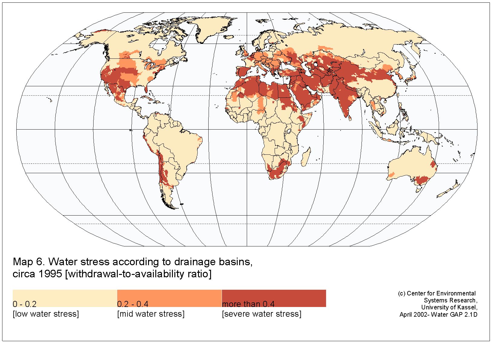
Cite this article
Largier, J.L. Recognizing Low-Inflow Estuaries as a Common Estuary Paradigm. Estuaries and Coasts 46, 1949–1970 (2023). https://doi.org/10.1007/s12237-023-01271-1
Received:
Revised:
Accepted:
Published:
Issue Date:
DOI: https://doi.org/10.1007/s12237-023-01271-1