
Abstract
In contrast to marine deposits, continental deposits in China are characterized by diverse sedimentary types, rapid changes in sedimentary facies, complex lithology, and thin, small sand bodies. In seismic sedimentology studies on continental lacustrine basins, new thinking and more detailed and effective technical means are needed to generate lithological data cubes and conduct seismic geomorphologic analyses. Based on a series of tests and studies, this paper presents the concepts of time-equivalent seismic attributes and seismic sedimentary bodies and a “four-step approach” for the seismic sedimentologic study of continental basins: Step 1, build a time-equivalent stratigraphic framework based on vertical analysis and horizontal correlation of lithofacies, electrofacies, seismic facies, and paleontological combinations; Step 2, further build a sedimentary facies model based on the analysis of single-well facies with outcrop, coring, and lab test data; Step 3, convert the seismic data into a lithological data cube reflecting different lithologies by means of seismic techniques; and Step 4, perform a time-equivalent attribute analysis and convert the planar attribute into a sedimentary facies map under the guidance of the sedimentary facies model. The whole process, highlighting the verification and calibration of geological data, is an iteration and feedback procedure of geoseismic data. The key technologies include the following: (1) a seismic data-lithology conversion technique applicable to complex lithology, which can convert the seismic reflection from interface types to rock layers; and (2) time-equivalent seismic unit analysis and a time-equivalent seismic attribute extraction technique. Finally, this paper demonstrates the validity of the approach with an example from the Qikou Sag in the Bohai Bay Basin and subsequent drilling results.
1 Introduction
Since it was presented for the first time in the 1990s (Zeng et al. 1998a, b), seismic sedimentology has been improved in theory and methodology by many researchers and is playing an increasingly important role in oil and gas exploration and development (Posamentier 2002; Miall 2002; Zeng and Hentz 2004; Zhang et al. 2007; Zhu et al. 2009; Zeng 2010; Reijenstein et al. 2011; Hubbard et al. 2011). Early seismic sedimentology research mainly focused on discussions of the cases and workflows of overseas marine basins (Kolla et al. 2001; Hentz and Zeng 2003; Zeng and Hentz 2004; Loucks et al. 2011) and established two key techniques: 90° phase shifting of seismic traces and strata slicing (Zeng 2011). The concept of seismic sedimentology was introduced in China in approximately 2000, followed by the study of sedimentary facies in China’s continental basins (Dong et al. 2006; Lin et al. 2007; Zhang et al. 2010; Zhu et al. 2011). However, few case studies have been reported; geologic researchers in China have mainly explored the applicability of seismic sedimentology for different types of continental basins in China and constructed seismic sedimentology models for different sedimentary types (Zhu et al. 2013). In practice, the existing workflows and key techniques were not fully suitable for the continental basins in China (Zeng 2011; Qian 2007). Therefore, we present a seismic sedimentology research method and workflow for the sedimentary features of the continental basins and demonstrate the efficacy of the method and its workflow using cases in the Qikou Sag in the Bohai Bay Basin and subsequent well drilling.
2 Sedimentary features of strata in continental basins and the difficulties of seismic sedimentology studies
It is well recognized by researchers in China that the seismic sedimentology method originally used for marine basins can provide useful guidance for studying the sedimentation of continental basins in this country (Zhao et al. 2011; Huang et al. 2011; Dong et al. 2011; Zeng et al. 2013). However, compared to marine basins, continental basins in China are quite different in their major control factors and petrophysical and seismic reflection features (Gu et al. 2005; Zeng et al. 2012) (Table 1), resulting in difficulties in seismic sedimentology interpretation due to the following characteristics: (1) complex depositional systems, various sedimentation types, and rapid changes in sedimentary facies within a small range; due to the filtering effect of wavelets, sands of different sedimentary types are similar in their geophysical responses, which is not only shown in seismic reflection but also on seismic slices, so a seismic sedimentology methodology for sands of different sedimentary types is still lacking; (2) thin and poor lateral continuity of sand bodies; seismic sedimentology investigates the sedimentary features and evolutionary pattern of deposition, but due to the effects of different deposition velocities in different parts of the basin, seismic slices for thin sands are prone to diachroneity; and (3) complex lithology–wave impedance relations; in contrast to marine basins, continental basins in China are much more complex in their lithological distribution (in many cases, conglomerate, sandstone, mudstone, limestone, and coal coexist) and multi-polar in wave impedance, making it difficult to calibrate the lithology on the 90° phase seismic profile and resulting in multiple possible interpretations of the lithology based on seismic data. In view of these constraints, new thinking and more detailed and effective technical means are needed to generate lithological data cubes and conduct seismic geomorphological analyses for continental basins.
3 Seismic sedimentology research method for continental rifted basins
In line with the sedimentary features of continental basins, the basic research approach to seismic sedimentology is “geology → seismic → geology” (Wei et al. 2011). Expressed as “point → plane → cube”, the approach stresses the calibration of geological data, which is also an effective way to resolve seismic ambiguity (Xu et al. 2010, 2011). The method can be summarized into four steps:
-
(1)
Build a time-equivalent stratigraphic framework. First, through detailed vertical analysis and horizontal correlation of outcrop, core and logging data, identify the high-order discontinuity surfaces, abrupt boundary changes in sedimentary facies and marine flooding or lake extension boundary resulting from changes in sea (lake) level or sedimentary base level, and, combined with the analysis of 3D seismic data, build a high-resolution stratigraphy sequence framework. The precision of sequence division depends on the data quality. When the geological and geophysical data are high in resolution, third- and fourth-order (or even higher) sequences and depositional system tracts can be recognized. Then, when time-equivalent analysis is conducted on divided seismic reflectors, adjust the diachronous horizons according to the analysis results. Finally, build the well-seismic tied time-equivalent stratigraphic framework.
-
(2)
Analyze the sedimentary facies of coring intervals in a single well by using the surface outcrop data, coring data, and lab test results. Use the analysis results to calibrate the SP, GR, etc., logs of the coring intervals and represent the sedimentary facies in the form of logs. Then, use these logs to study the sedimentary facies of non-coring intervals, thus accomplishing the sedimentary facies analysis of the target interval (single-well facies division), and build the sedimentary facies model.
-
(3)
Convert the seismic data cube into a lithological data cube with wave impedance, SP, and GR via seismic data conversion (i.e., reservoir parameter inversion or 90° phase shifting).
-
(4)
Conduct time-equivalent stratal slicing or extract the time-equivalent unit’s seismic attributes, and under the guidance of the sedimentary facies model, interpret these data cubes based on continuous vertical changes and relative spatial changes in the time-equivalent attributes. Obtain a relatively accurate sedimentary facies plan and profile, and finally build a 3D depositional system model based on modeling and 3D visualization (Fig. 1).
Fig. 1 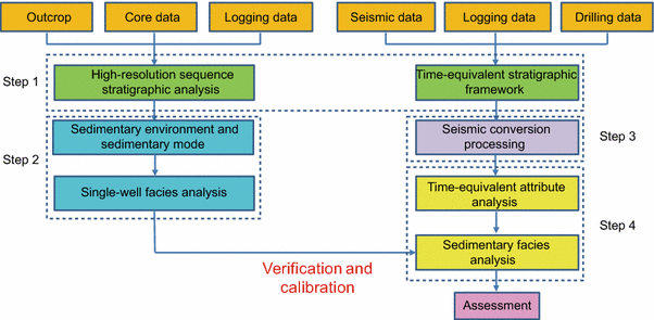
Seismic sedimentology research approach and method for continental basins

The method for seismic sedimentology research in continental basins involves two major techniques: (1) time-equivalent seismic unit analysis and a time-equivalent seismic attribute extraction technique; (2) a seismic data-lithology conversion processing technique.
3.1 Time-equivalent seismic unit analysis and time-equivalent seismic attribute extraction technique
3.1.1 Interpretation risks caused by seismic slice diachroneity
Time-equivalent stratigraphy is the foundation for sedimentary analysis. Among the several slicing techniques commonly used at present, stratal slicing is closer to time-equivalent interfaces than time slicing and horizon slicing. However, even stratal slicing is prone to diachroneity.
Stratal slicing assumes that the vertically equal ratio division between two time-equivalent sedimentary interfaces is approximate to slicing along time-equivalent sedimentary interfaces. This assumption assumes that the deposition velocity in the vertical direction does not change with time. However, deposition velocity is affected by factors such as sediment supply rate and changes in accommodation, and these factors change with time due to the effects of tectonic movements and paleoclimate, among other variables. Thus, any geological process is a multivariate function including the time variable. For any point on a plane, the structure and sedimentary environment constantly change with time; thus, the deposition velocity at this point changes with time. Moreover, in many cases, the effects of this change on deposits in continental basins are not negligible (Lin and Zhang 2006), which is different from deposits in marine basins. In addition, the virtual 3D model built by Zeng et al. (1998a, b) reveals that in the 30 Hz Ricker wavelet synthetic data, the stratal slices controlled by two marker events have a left or right deviation of approximately 9 ms. Thus, diachroneity is likely to occur in stratal slices of thin continental interbeds.
Diachronous stratal slices complicate interpretation and are likely to lead to misinterpretations. Figure 2 shows the theoretical model of the fourth-period channel, in which the maximum thickness of the channel sands is 3 m, the maximum width of the channel is 50 m, and the velocities of the first-period, second-period, third-period, and fourth-period channel sands are 1,800 m/s, 1,700 m/s, 1,600 m/s, and 1,500 m/s, respectively. The mudstone is 4 m thick, and its velocities, from shallow to deep, are 1,000 m/s, 1,200 m/s, 1,400 m/s, 1,600 m/s, and 1,800 m/s. Figure 2a shows the model perpendicular to the channel. Figure 2b–e shows the planar geometry of the four periods of the channel (corresponding to slices 1, 2, 3, and 4, respectively, in Fig. 2a). Figure 2f is a 20 Hz Ricker wavelet synthetic section (corresponding to Fig. 2a). Slice A, as shown in Fig. 2g, picks the top of the wave crest corresponding to the location of the fourth-period channel. Affected by the seismic resolution and sand shale velocity difference, there is up to a 6 ms error between the geological time-equivalent surface of slice A and that corresponding to the fourth-period channel (slice B position). Compared with slice B (Fig. 2h), slice A can be interpreted in a variety of ways due to the interference of adjacent layers, but it is difficult to identify a real situation in which only one meandering river channel exists.

Theoretical model of four periods of a channel. a The model perpendicular to the channel, b–e the planar geometry of the four periods of the channel (corresponding to slices 1, 2, 3, and 4), f a 20 Hz Ricker wavelet synthetic section (corresponding to (a)), g corresponding to slice A, and h corresponding to slice B
3.1.2 Time-equivalent slice processing technique
Local diachroneity on stratal slices can be removed by non-linear processing. Figure 3a shows a stratal slice of the first member of the Nenjiang Formation in the Anda area of the Songliao Basin, where two nearly NS channels in the study area developed and the channel in the middle-eastern area divided in the middle. To determine the reason for this phenomenon, we analyzed the isochronism of seismic reflection at the break in the channel. Zeng et al. (1998a, b) asserted that the occurrence of time-equivalent reflection events did not change with seismic frequency. Generally, a series of filters are used for filtering in the seismic band width. If the occurrence of a seismic event is not related to its frequency, the event is time-equivalent; otherwise, it is diachronic. Therefore, the seismic reflection dip angles of different frequencies can be subtracted. If the difference is nearly zero, the seismic reflection is time-equivalent. Figure 3b shows the dip difference profile of profile A crossing the channel break (see Fig. 3a for the profile position). The dip angle difference at the channel break is approximately 6°, showing an obvious diachronous feature. To obtain time-equivalent stratal slices, non-linear processing can be conducted on the stratal slice at the channel break. The original slice was obtained by interpolation between the two time-equivalent layers T1 and T2. In this case, we used a Gaussian function to interpolate between the two time-equivalent layers at the break (area in the black circle in Fig. 3a). Figure 3d shows the slice position after non-linear processing, with a dip angle difference close to zero. Figure 3c is the amplitude slice after non-linear processing, which shows that the channel break has apparently improved.

Stratal slice and time-equivalent analysis profile for the 1st member of the Nenjiang Fm. in the Anda area of the Songliao Basin. a A stratal slice of the first member of the Nenjiang Formation in the Anda area of the Songliao Basin, b the dip difference profile of profile A crossing the channel break, c the amplitude slice after non-linear processing, and d the dip difference profile of profile A, showing the slice position after nonlinear processing, with a dip angle difference close to zero
3.1.3 Analysis of time-equivalent seismic unit
Because continental sands are thin and exhibit rapid facies changes, their stratal slices have universal diachroneity, which makes it impossible to obtain time-equivalent stratal slices through non-linear processing. In this case, the vertical study scale should be adjusted to increase the time unit thickness. For this purpose, we proposed the concept of a time-equivalent seismic unit. A time-equivalent seismic unit refers to the comprehensive responses of a sedimentary body from a certain geological period on the seismic reflection data volume; the top and bottom of a time-equivalent seismic unit are sedimentary time-equivalent planes that can be identified by seismic data.
Based on high-resolution stratigraphic sequence analysis, it is possible to classify four or more orders of sequence and depositional system tracts. The sequence units correspond to time-equivalent seismic units. High-order sequence units correspond to the minimum time-equivalent seismic units that can be analyzed. The tops and bottoms of these sequences generally correspond to the lake expansion boundaries, which have relatively stable lateral distribution and feature strong reflection, good continuity on the seismic profile, and good isochronism of corresponding seismic slices. In contrast, the sand bodies inside the sequence are generally thin and unstable in distribution, appearing as discontinuous reflections on the seismic profile.
3.1.4 Extraction of time-equivalent seismic attributes
To analyze the sedimentation distribution features of the time-equivalent seismic unit, it is necessary to introduce the concepts of time-equivalent seismic attributes and seismic sedimentary bodies. The time-equivalent seismic attribute represents the geometric, kinematics, dynamic, and statistical features of seismic waves corresponding to the time-equivalent seismic unit. The seismic sedimentary body is a reflection of a sedimentary event on the seismic record. In addition to thin sands that cannot be analyzed by stratal slices, gravity flow events exhibit diachroneity in certain cases. Thus, conventional stratal slicing or interlayer seismic attributes can hardly ensure the isochronism of attribute slices, and the time-equivalent seismic unit can ensure the study unit’s unity with time. The extracted time-equivalent seismic attribute reflects the seismic reflection features of the predominant facies in this interval. The planar distribution feature of the time-equivalent seismic attribute provides the base map for sedimentation analysis and overcomes the diachroneity that commonly occurs in continental deposits. When the length of the time-equivalent unit time window approaches zero, the time-equivalent seismic attribute equals the time-equivalent stratal slice. Hence, the time-equivalent stratal slice can be regarded as a particular case of the time-equivalent seismic attribute.
Figure 4 shows a 90° phase shifting profile through Well X3 in the Qinan sub-sag of the Qikou Sag (see Fig. 5 for the position of the plane). The core data of Well X3 show that gravity flow sands in the SS1 sequence developed there due to their strong scouring and incision effects. The seismic sedimentary body corresponding to the sands exhibits upwarp at both ends and is concave in the middle. On the original seismic profile with relatively low predominant frequency (17 Hz) and the frequency-division profile of 40 Hz, the seismic sedimentary body is consistent in occurrence, indicating that the sand is syndeposited, but on the stratal slice, there is an obvious event-crossing phenomenon without time-equivalent meaning and thus without meaning for seismic sedimentology analysis. Therefore, a time-equivalent seismic attribute extraction was conducted.

90° phase shifting profile of the profile AB through Well X3 in the Qinan subsag (see Fig. 5 for the position of profile AB)

Maximum peak amplitude of SS1 in the Shahejie Formation of the Qikou Sag
Figure 5 shows the maximum peak amplitude of the SS1 sequence; the higher the amplitude, the better developed is the sand. The attribute shows there are two sand strips in a nearly NS direction in the western part of the work area, and there is a fan-shaped sand body in the eastern part of the work area. The attribute distribution matches fully with the sands revealed by drilling. Well X3 is in the middle strip, showing that these strips are gravity flow channels, and the fan body in the eastern part is a sub-lacustrine fan.
3.2 Seismic data lithological conversion technique
It is a prerequisite of seismic sedimentology research to convert the seismic data cube into a lithological data cube that can be directly correlated with logging data. Zeng and Backus (2005a, b) demonstrated the advantages of the 90° phase shifting of seismic data in the stratigraphic and lithological interpretation of thin beds by means of models and examples and concluded that the 90° phase wavelet shifted the main lobe (maximum amplitude) of the seismic response to the midpoint of the thin beds. Thus, the seismic response corresponded to the midpoint of the thin bed rather than its top and bottom boundaries, connecting the main seismic event to the reservoir unit defined in geology (e.g., sandstone reservoir). In this way, the seismic polarity can correspond to lithology within 0–1 wavelength ranges. Although the inaccuracy increases when the formation thickness is less than ¼ λ (λ is wavelength), the top and bottom boundaries of the formation can be determined at the position where the amplitude passes the zero point. When applying these improvements to real data, a one-to-one relationship will be established between the seismic event and the lithological unit of the thin beds, which will facilitate the seismic interpretation of sedimentary lithology (e.g., distinguishing sand from shale).
When the wave impedance can be used to effectively distinguish the lithology, the 90° phase shifting of seismic data is undoubtedly the most economic and effective seismic lithological method at present. However, in contrast to marine basins, the continental basins in China have multiple provenances, complex lithology, poor sorting, and a complicated lithology–wave impedance relationship, which make it difficult to interpret their lithology based on 90° phase shifting.
One possible solution is to convert the seismic data into a logging parameter data cube capable of reflecting the lithology (Su et al. 2013), which involves the following steps: (1) analyze the reservoir features and choose the logging data that best reflect the reservoir features in the work area; (2) perform detailed well-seismic calibration and convert the seismic data into a 90° phase data cube; and (3) take the 90° phase shifting data cube as the constraint cube and use the co-kriging and fractal interpolation reconstruction methods to accomplish the seismic trace logging parameter inversion. Constraint data cubes constrained by a 90° phase conversion data cube have two advantages: first, their amplitude fidelity, i.e., the amplitude of the original seismogram, is maintained; second, they have closely corresponding spatial positions with equivalent reservoirs (equivalent layers of a number of reservoirs).
The fractal theory provides an effective tool for the description of complex phenomena. Well logging and seismic signals have self-similarity, i.e., fractal features (Lu and Li 1996; Jiang et al. 2006). The fractional Brownian motion (FBM), a statistically self-similar and non-stationary random process, is currently one of the most common mathematical models used to study fractal signals and has been applied effectively in reservoir fracture prediction and high-resolution processing (Leary 1991; Cao et al. 2005; Li and Li 2008; Li et al. 2008; Chang and Liu 2002; Fen et al. 2011; Huang et al. 2009). In the present paper, FBM is applied in seismic lithological inversion.
In probability theory, a normalized FBM of Hurst index α (0 < α<1) is defined as X: [0, ∞) → R, a “Random Walk Process” within a certain probability space, which causes FBM to satisfy the following:
-
(1)
with probability 1, X(0) = 0 and X(t) is a continuous function of t,
-
(2)
for t ≥ 0 and h > 0, the increment X(t + h)−X(t) is subject to normal distribution with a mean of 0 and variance h 2a; thus,
$$ P(X(t + h) - X(t) \le x) = (2\uppi)^{ - 1/2} h^{ - a} \int_{ - \infty }^{x} {\exp \left( {\frac{{ - u^{2} }}{{2h^{2a} }}} \right){\text{d}}u} $$(1)B a (t) is generally used to denote an FBM of Hurst index α.
Pentland (1984) extended FBM to a high-dimensional situation and defined the fractional Brownian random field (FBR): with X, ΔX∈R 2, 0 ≤ H≤1, F(y) is a Gaussian random function with a mean of 0, P r(•) represents the probability measure and ‖•‖ represents the norm. If the random field B H (X) meets
the B H (X) is the FBR and is characterized by
Then, the parameter H can be calculated conveniently using Eq. (3).
Essentially seismic lithological inversion is the joint application of the kriging technique and fractal interpolation. The co-kriging interpolation result is faithful to well point data and seismic lateral changes (Yang et al. 2012; Huang et al. 2012). The random fractal interpolation methods consist mainly of random midpoint shift, continuous random stacking, and spectrum synthesis. In this paper, the random midpoint shift interpolation method is used, which is in fact a recursive midpoint displacement method, with the following computing equations:
where X l is a linear term representing large-scale feature information and is worked out using the co-kriging method; PA is a co-kriging interpolation operator; A is a data cube of 90° phase conversion; and D i represents well data. When the geological condition is simple, X l can also be derived using the linear interpolation method.
X n is a non-linear term, representing medium- and small-scale feature information; G is a Gaussian random variable and follows the distribution of N (0, 1); σ is a standard variance of the normal distribution of data; H is the Hurst index depicting the detail and roughness of the data information; ‖ΔX‖ is a sample interval; and K is the calibration coefficient of the non-linear term. We can see that the value of the interpolation point completely depends on the H index and σ characterizing the raw data. Therefore, the ultimate inversion results would closely match the well point data and seismic horizontal changes, and the vertical resolution is consistent with the well logging data.
4 Case study
4.1 Overview of the 3D study area
The study area, located in the Qibei sub-sag of the Qikou Sag, is a Cenozoic rifted basin (Zhou et al. 2011). The Sha2 member is the target zone for study and has a burial depth of 4,100–5,000 m, a reservoir (single layer) thickness of less than 12 m, and a lithology of sandstone, mudstone, calcareous mudstone, and dolomite interbeds with unequal thicknesses. In recent years, high-yielding oil and gas wells in the Sha2 member have been discovered in this area; thus, there is an urgent need to understand the reservoir distribution and sedimentary pattern. However, the predominant frequency of seismic data in this area is approximately 17 Hz; this resolution does not meet the demand for distinguishing thin interbed reservoirs less than 12 m thick. Moreover, due to the existence of calcareous mudstone, it is also difficult to distinguish sandstone from calcareous mudstone using the wave impedance absolute value. As a result, it is difficult to reflect the variation of the sedimentary reservoir by seismic slices. Therefore, the co-kriging and fractal theory-based lithology conversion technique and the seismic sedimentology research method for continental basins are utilized in this study to determine the spatial distribution and sedimentary features of the reservoirs.
4.2 Building the time-equivalent stratigraphic framework
Substantial research has been conducted on the Paleogene sequence division of the Qikou Sag (Wu et al. 2010; Huang et al. 2010), which concluded that the Sha2 member is a complete third-order sequence with an angular unconformity at the basin margin and a conformable contact in the central basin. The Sha2 member can be further divided into three fourth-order sequences, i.e., BinII (SB2), BinIII (SB3), and BinIV (SB4). The final sequence interpretation scheme is obtained based on the correlation and the verification of the seismic profile with the sequence interpretation scheme on well logs after a depth-time conversion.
With the AA′ profile that extends in the dip direction as an example (Fig. 6), the sequence boundary shows continuous seismic reflections. These reflections are mostly parallel to the maximum flooding surface, and their occurrence does not change with frequency, thereby exhibiting time-equivalent stratigraphy significance. The building of the sequence framework is not only a prerequisite for time-equivalent stratal slicing but also provides constraint conditions for seismic lithology conversion.

Sequence division of the Sha2 member based on the AA′ well-tie seismic profile in the Qibei sub-sag
4.3 Single-well facies analysis
Carbon dust and plant stem fossils occur commonly in the coring intervals of the Sha2 member in the study area. The mudstone is mainly gray and grayish-green, indicating that the Sha2 member was primarily deposited in shallow water and is dominated by coastal–shallow lacustrine deposits.
Based on the observation of cores taken from several key wells, fan delta front deposits are developed in the Sha2 member in the northern study area, e.g., gray mudstone dominates the lithology of Well W9 and massive gray packsand is developed in the middle and lower parts. Core observations also reveal plant stem carbon dust, boulder clay, and slump deformation structures along with sedimentary structures such as low-angle oblique bedding, trough cross bedding, and parallel bedding (Fig. 7). The lithological electric property features a tooth-like bell-type and tooth-like funnel-type GR log. The core facies is interpreted as a fan delta front deposit. The western and southwestern parts are dominated by beach bar sedimentary facies, where channel scouring structure is not obvious, the sandstone exhibits fine granularity and good sorting, and boulder clay with bioclasts resulting from storm events can be seen.

Log features and core photos of Well W9
4.4 Seismic data conversion
The efficacy of seismic amplitudes as lithological markers depends on the wave impedance difference between the different lithologies of layered media. Petrophysical analysis of several wells in the Qibei sub-sag indicates an insignificant wave impedance difference between different lithologies of the Sha2 member in the study area. The wave impedance of mudstone ranges from 7,200 to 14,400 (m/s g/cm3), with two peak values at 9,000 (m/s g/cm3) and 10,800 (m/s g/cm3). The wave impedance of sandstone ranges from 8,400 to 13,200 (m/s g/cm3), with a peak value at 11,400 (m/s g/cm3). For calcareous mudstone, the wave impedance ranges from 10,800 to 12,600 (m/s g/cm3), overlapping the peak value of sandstone. The reflection events in the 90° phase data cube fail to reach a close correspondence with different lithologies. Because the sand bodies are generally thin (less than 1/4 λ) and the wave impedance difference between sandstone and mudstone is insignificant, a reflection event may correspond to sandstone or mudstone on the 90° phase profile. Therefore, the 90° phase data cube is not a good lithological criterion for the complex lithology zones where the impedances of sandstone and mudstone are difficult to distinguish. The sedimentary evolutionary features are unlikely to be reflected in the stratal slices obtained from the 90° phase data cube. Figure 8 shows three stratal slices extracted from the 90° phase data cube (see Fig. 9 for their positions). Slices 1, 2, and 3 correspond to the lowstand system tract, lake transgressive system tract, and highstand system tract of the BinIII sequence (SB3), respectively. In the lake transgressive system tract, the sand body is not developed in Wells W2 and W3, which are located within the high-amplitude and low-amplitude zones of the stratal slices, respectively. In the lowstand system tract of the BinIII sequence, a thick sand body is developed in Wells W4, W5, and W6. In addition, the sand body is not developed in the lake transgressive system tract, whereas a thin sand body is developed in the highstand system tract, but the sedimentary evolution features are not reflected on the stratal slices.

Three stratal slices of the BinIII sequence extracted from the 90° phase data cube. Slices 1, 2, and 3 correspond to a lowstand system tract, lake transgressive system tract, and highstand system tract, respectively

NS-trending well-tie profile
The co-kriging and fractal theory-based seismic data conversion method described above is adopted to obtain a lithological data cube applicable in sedimentation analysis. First, the logging data capable of reflecting the reservoir features of the study area are selected. In this case, the shale content curve (Vsh) is determined based on GR. The shale content not only helps to distinguish reservoirs and non-reservoirs but also can reveal the hydrodynamic condition and thus contribute to the identification of the sedimentary environment. Second, detailed well-seismic calibration was performed, and seismic data were converted into a 90° phase data cube. Finally, under the constraint of the time-equivalent stratigraphic framework and taking the 90° phase shifting data cube as the constraint data cube, the co-kriging and fractal interpolation reconstruction methods were used to achieve the seismic trace lithological data inversion.
Figure 10 shows the inversion profile corresponding to Fig. 6. The inversion results obtained by the above methods have the following features: (1) Different lithologies are effectively discriminated, and the details of the original seismic data’s horizontal changes are kept. Because the inversion values completely depend on the H index, σ, and co-kriging interpolation values describing the original data, the horizontal change features of the original seismic profile are better kept in the inversion results, and the inherent modeling features of a well-constrained inversion are overcome, thereby laying a solid foundation for the lithological data cube to reflect the change in sedimentation. Figure 6 and Fig. 10 show three major change points. Change points 1 and 2 show reflection peaks on the seismic profile. As indicated by the shale content curve, the reservoir is not developed at change point 1 but is better developed at change point 2. This issue is resolved perfectly by inversion. At change point 3, the seismic reflection weakens gradually from west to east, its wave form becomes poorer in continuity, the number of sand bodies increases from west to east on the corresponding inversion profile, and the sand body is lens-like, showing a consistent change with seismic wave form. (2) The resolution is enhanced by inversion. Due to the supplementary high-frequency logging information, the resolution for various lithologies and strata is enhanced significantly on the inversion lithological profile, and the inversion results match perfectly with the logging data.

AA′ inversion profile of the Qibei sub-sag
4.5 Time-equivalent seismic attribute and seismic sedimentology analysis
Inversion effectively discriminates various lithologies, enhances the resolution of the lithological data cube, greatly reduces the thickness of the minimal mapping unit, and provides conditions for using the time-equivalent slice to study the sedimentation change. To facilitate analysis and correlation, three slices of the BinIII sequence corresponding to slices 1, 2, and 3 were interpreted. These slices describe the distribution and interrelationship of the BinIII lowstand system tract, lake transgressive system tract, and highstand system tract deposits. Figure 11 shows their accurate locations on profile BB′. In this figure, red and yellow represent sandstone, green represents argillaceous sandstone, and blue represents mudstone.

NS-trending lithological profile BB′ showing the locations of three stratal slices
Slice 1 in Fig. 12 is the stratal slice of a lowstand system tract, containing three sand bodies in a fan shape. Fan body 1 developed in the northeastern part and has the widest distribution range. This fan body is distributed from north to southeast and southwest and intersects with fan body 3 in a fault south of Well W4. Fan body 3 is mainly distributed in the southeastern part of the study area. Fan body 2 developed in the northwestern part and has three lobes extending toward the south. Drilling cores and mud logging results indicate that these fan bodies are mostly interbeds of gray packsand and siltstone, with a single-layer thickness of 4–8 m. The GR log represents a combination of tooth-like funnel-type and tooth-like bell shapes in Well W4, a tooth-like shape in W5, and a funnel-type shape in W6. Wells W4 and W6 are located in the red and yellow zones, whereas W5 is in the green zone. Depositional model analysis shows that Wells W4, W5, and W6 are a fan delta front distributary channel, river mouth bar, and interchannel deposit, respectively. A small area of argillaceous sandstone is distributed parallel to the lake shoreline in the southwestern part and is interpreted as coastal beach bar sand.

Three strata slices of the BinIII sequence extracted from the lithological data cube. Slices 1, 2, and 3 correspond to a lowstand system tract, lake transgressive system tract, and highstand system tract, respectively
Slice 2 in Fig. 12 is the stratal slice of a lake transgressive system tract, indicating that the sand bodies retrograded toward the basin margin as the lake area increased. In the study area, sparse sand bodies are distributed only parallel to the lake shoreline in the southwestern part and are interpreted as beach bar sand. Gray shale occurs in Wells W1, W2, W3, W4, W5, and W6, which feature straight GR log curves.
Slice 3 in Fig. 12 is the stratal slice of a highstand system tract, indicating that the lake level dropped and the delta prograded gradually in this period. Two fan bodies in the same location as the lowstand system tract appear in the northern part of the slice. Compared with the period of the lowstand system tract, the scale of these fan bodies decreased. The fan body in the east comprises three lobes. Log curves show a coarsening-upward funnel shape in Well W6, tooth-like funnel shape in W5, and tooth shape in W4. A beach bar sand body is developed in the southwestern part.
The depositional model observed on these three slices corresponds well with the sequence evolution stage and the drilling results, thereby demonstrating the reliability of the new seismic lithology method. Moreover, fan body 3, located in the south, was confirmed by later drilling.
5 Conclusions
Continental basins differ greatly from marine basins in the major control factors of their structure, sedimentation and sequence formation, petrophysical features, and seismic reflection features. Therefore, new methods and techniques for seismic sedimentology research on continental basins must be developed.
Seismic sedimentology research on continental basins should highlight the verification and calibration of geological data. In this paper, we present the concepts of time-equivalent seismic attributes and seismic sedimentary bodies as well as seismic data-lithology conversion processing and time-equivalent seismic attribute extraction methods and techniques. On this basis, we introduce a “four-step” approach applicable to seismic sedimentology research on continental basins.
Using the methods discussed above, seismic sedimentology research was conducted for the Qikou Sag in the Bohai Bay Basin. The research results show that the Sha2 member, where deltaic deposits are developed, is a potential site for future exploration. The above findings have been confirmed by subsequent drilling, thereby demonstrating the reliability and validity of the methods and techniques introduced in this paper.
References
Cao MS, Ren QW, Wang HH. A method of detecting seismic singularities using combined wavelet with fractal. Chin J Geophys. 2005;48(3):672–9 (in Chinese).
Chang X, Liu YK. The generalized fractal dimension of seismic records and its application. Chin J Geophys. 2002;45(6):839–46 (in Chinese).
Dong CM, Zhang XG, Lin CY. Discussions on several issues about seismic sedimentology. Oil Geophys Prospect. 2006;41(4):405–9 (in Chinese).
Dong YL, Zhu XM, Hu TH, et al. Research on seismic sedimentology of He-3 Formation in Biyang Sag. Earth Sci Front. 2011;18(2):284–93 (in Chinese).
Fen ZD, Dai JS, Deng H, et al. Quantitative evaluation of fractures with fractal geometry in Kela-2 gas field. Oil Gas Geol. 2011;32(6):928–33 (in Chinese).
Gu JY, Guo BC, Zhang XY. Sequence stratigraphic framework and model of the continental basins in China. Pet Explor Dev. 2005;32(5):11–5 (in Chinese).
Hentz TF, Zeng HL. High-frequency Miocene sequence stratigraphy, offshore Louisiana: Cycle framework and influence on production distribution in a mature shelf province. AAPG Bull. 2003;87(2):197–230.
Huang CY, Wang H, Wu YP, et al. Analysis of the hydrocarbon enrichment regularity in the sequence stratigraphic framework of Tertiary in Qikou Sag. J Jilin Univ (Earth Sci Ed). 2010;40(5):986–95 (in Chinese).
Huang HD, Cao XH, Luo Q. An application of seismic sedimentology in predicting organic reefs and banks: A case study on the Jiannan-Longjuba region of the eastern Sichuan fold belt. Acta Pet Sin. 2011;32(4):629–36 (in Chinese).
Huang YP, Dong SH, Geng JH. Ordovician limestone aquosity prediction using nonlinear seismic attributes: case from the Xutuan coal mine. Appl Geophys. 2009;6(4):359–66.
Huang ZY, Gan LD, Dai XF, et al. Key parameter optimization and analysis of stochastic seismic inversion. Appl Geophys. 2012;9(1):49–56.
Hubbard SM, Smith DG, Nielsen H, et al. Seismic geomorphology and sedimentology of a tidally influenced river deposit, Lower Cretaceous Athabasca oil sands, Alberta, Canada. AAPG Bull. 2011;95(7):1123–45.
Jiang SH, Chen JY, Jiang Y, et al. Fractal dimension calculation of seismic traces and application to reservoir description in coastal regions. Period Ocean Univ China. 2006;36(5):841–4 (in Chinese).
Kolla V, Bourges P, Urruty JM, et al. Evolution of deep-water Tertiary sinuous channels offshore Angola (west Africa) and implications for reservoir architecture. AAPG Bull. 2001;85(8):1373–405.
Leary PC. Deep borehole log evidence for fractal distribution of fractures in crystalline rock. Geophys J Int. 1991;107(3):615–27.
Li W, Yan T, Bi XL. Mechanism of hydraulically created fracture breakdown and propagation based on fractal method. J China Univ Pet. 2008;32(5):87–91 (in Chinese).
Li XF, Li XF. Seismic data reconstruction with fractal interpolation. Chin J Geophys. 2008;51(4):1196–201 (in Chinese).
Lin CY, Zhang XG. The discussion of seismic sedimentology. Adv Earth Sci. 2006;21(11):1140–4 (in Chinese).
Lin CY, Zhang XG, Dong CM. Concepts of seismic sedimentology and its preliminary application. Acta Pet Sin. 2007;28(2):69–71 (in Chinese).
Loucks RG, Moore BT, Zeng HL. On-shelf lower Miocene Oakville sediment-dispersal patterns within a three-dimensional sequence-stratigraphic architectural framework and implications for deep-water reservoirs in the central coastal area of Texas. AAPG Bull. 2011;95(10):1795–817.
Lu JA, Li ZB. The self-similarity study of well logging curves. Well Logging Technol. 1996;20(6):422–7 (in Chinese).
Miall AD. Architecture and sequence stratigraphy of Pleistocene fluvial systems in the Malay Basin, based on seismic time-slice analysis. AAPG Bull. 2002;86(7):1201–16.
Pentland AP. Fractal-based description of natural scenes. IEEE Trans Pattern Anal Mach Intell. 1984;6(6):661–74.
Posamentier HW. Ancient shelf ridges, a potentially significant component of the transgressive systems tract: case study from offshore northwest Java. AAPG Bull. 2002;86(1):75–106.
Qian RJ. Analysis of some issues in interpretation of seismic slices. Oil Geophys Prospect. 2007;42(4):482–7 (in Chinese).
Reijenstein HM, Posamentier HW, Bhattacharya JP. Seismic geomorphology and high-resolution seismic stratigraphy of inner-shelf fluvial, estuarine, deltaic, and marine sequences, Gulf of Thailand. AAPG Bull. 2011;95(11):1959–90.
Su MJ, Wang XW, Yuan SQ. Seismic sedimentologic analysis and its application in areas with complex lithology—Case study on Qibei Sag in Huanghua Depression. SEG International Exposition and 83rd Annual Meeting. 2013, 22-27 September, Houston, Texas.
Wei PS, Li XB, Yong XS, et al. Discussion on petroleum seismogeology. Lithol Reserv. 2011;23(3):1–6 (in Chinese).
Wu YP, Yang CY, Wang H, et al. Integrated study of tectonics—sequence stratrigraphy—sedimentology in the Qikou Sag and its application. Geotectonica et Metallogenia. 2010;34(4):451–60 (in Chinese).
Xu HN, Yang SX, Zheng XD, et al. Seismic identification of gas hydrate and its distribution in Shenhu Area, South China Sea. Chin J Geophys. 2010;53(7):1691–8 (in Chinese).
Xu Y, Shu P, Ji XY. A research on object-control geology modeling of volcano reservoir with seismic and logging data in Xushen gas field. Chin J Geophys. 2011;54(2):336–42 (in Chinese).
Yang K, Ai DF, Geng JH. A new geostatistical inversion and reservoir modeling technique constrained by well-log, crosshole and surface seismic data. Chin J Geophys. 2012;55(8):2695–704 (in Chinese).
Zeng HL. Geologic significance of anomalous instantaneous frequency. Geophysics. 2010;75(3):P23–30.
Zeng HL. Seismic sedimentology in China: a review. Acta Sedimentol Sin. 2011;29(3):417–26 (in Chinese).
Zeng HL, Backus MM. Interpretive advantages of 90 degrees–phase wavelets: part 1—modeling. Geophysics. 2005a;70(3):C7–15.
Zeng HL, Backus MM. Interpretive advantages of 90 degrees–phase wavelets: part 2—seismic applications. Geophysics. 2005b;70(3):C17–24.
Zeng HL, Hentz TF. High-frequency sequence stratigraphy from seismic sedimentology: applied to Miocene, Vermilion Block50, Tiger Shoal area, offshore Louisiana. AAPG Bull. 2004;88(2):153–74.
Zeng HL, Backus MM, Barrow KT. Stratal slicing, part I: realistic 3-D seismic model. Geophysics. 1998a;63(2):502–13.
Zeng HL, Henry SC, Riola JP. Stratal slicing, part II: real seismic data. Geophysics. 1998b;63(2):514–22.
Zeng HL, Zhu XM, Zhu RK, et al. Guidelines for seismic sedimentologic study in non-marine postrift basins. Pet Explor Dev. 2012;39(3):275–84 (in Chinese).
Zeng HL, Zhu XM, Zhu RK, et al. Seismic prediction of sandstone diagenetic facies: applied to Cretaceous Qingshankou Formation in Qijia Depression, Songliao Basin. Pet Explor Dev. 2013;40(3):266–74 (in Chinese).
Zhang JH, Zhou ZX, Tan MY, et al. Discussions on several issues in seismic slice interpretation. Oil Geophys Prospect. 2007;42(3):348–52 361 (in Chinese).
Zhang XG, Lin CY, Zhang T. Seismic sedimentology and its application in shallow sea area, gentle slope belt of Chengning Uplift. J Earth Sci. 2010;21(4):471–9.
Zhao WZ, Zou CN, Chi YL, et al. Sequence stratigraphy, seismic sedimentology, and lithostratigraphic plays: Upper Cretaceous, Sifangtuozi area, southwest Songliao Basin, China. AAPG Bull. 2011;95(2):241–65.
Zhou LH, Pu XG, Zhou JS, et al. Sand-gathering and reservoir-controlling mechanisms of Paleogene slope-break system in Qikou Sag, Huanghua Depression, Bohai Bay Basin. Pet Geol Exp. 2011;33(4):371–7 (in Chinese).
Zhu XM, Dong YL, Hu TH, et al. Seismic sedimentology study of fine sequence stratigraphic framework: a case study of the Hetaoyuan Formation in the Biyang Sag. Oil Gas Geol. 2011;32(4):615–24 (in Chinese).
Zhu XM, Li Y, Dong YL, et al. The program of seismic sedimentology and its application to Shahejie Formation in Qikou Depression of North China. Geol China. 2013;40(1):152–62 (in Chinese).
Zhu XM, Liu CL, Zhang YN, et al. Application of seismic sedimentology in prediction of non-marine lacustrine deltaic sand bodies. Acta Sedimentol Sin. 2009;27(5):915–21 (in Chinese).
Acknowledgments
This research was supported by the Key Scientific and Technological Project “Seismic-Sedimentology Software System Investigation and Application” of PetroChina Company Limited (2012B-3709). The authors would like to take this opportunity to express our appreciation and thanks to Ni Changkuan, Cai Gang, and Zhang Zhaohui for their hard work on this study.
Author information
Authors and Affiliations
Corresponding author
Additional information
Edited by Jie Hao
Rights and permissions
Open Access This article is distributed under the terms of the Creative Commons Attribution License which permits any use, distribution, and reproduction in any medium, provided the original author(s) and the source are credited.
About this article

Cite this article
Wei, PS., Su, MJ. Methods for seismic sedimentology research on continental basins. Pet. Sci. 12, 67–80 (2015). https://doi.org/10.1007/s12182-014-0002-9
Received:
Published:
Issue Date:
DOI: https://doi.org/10.1007/s12182-014-0002-9