
Abstract
Porous Fe3O4 scaffolds were fabricated while subject to a low (7.8 mT) magnetic field applied in helical and Bouligand motions using a custom-built tri-axial nested Helmholtz coils-based freeze-casting setup. This setup allowed for the control of a dynamic, uniform low-strength magnetic field to align particles during the freezing process, resulting in the majority of lamellar walls aligning within ± 30° of the magnetic field direction and a decrease in porosity by up to 42%. Similar to how helical and Bouligand structures in nature promote impact resistance, these magnetic field motions produced structures with improved high strain rate mechanical properties. Strain at failure was increased by up to 2 times as cracks deflected to match the applied angles of rotation of the magnetic field.
Introduction
Helical and Bouligand structures are of particular interest as they tend to provide high impact resistance.1 Helical structures are characterized by their constant helical twisting around an axial direction and are found in structures such as a DNA strand, coil spring, or tropocollagen.2 Bouligand structures are characterized by oriented sheets of fibers or platelets that are stacked one on top of the other while being rotated in steps after each layer by a certain angle (e.g., 60°).3 Such structures are seen in a number of natural materials including the clubs of mantis shrimp and grasshopper exoskeletons, where impact resistance is a critical property for predation and protection, respectively.1,4 One fabrication technique to create materials inspired by these natural materials is freeze casting.
The freeze-casting fabrication technique uses the formation of ice crystals in a slurry to create porous scaffolds in a four-step process. First, a colloidal slurry is made using solid loading particles, a liquid freezing solvent, polymeric binders, and a dispersant. Second, the slurry is directionally frozen so as to segregate the solid particles between the growing ice crystals. Third, the frozen scaffolds are subjected to a low temperature and pressure to sublimate the grown ice crystals. Fourth, the resultant green bodies are sintered to fuse the solid particles together. The resultant porous structure of the scaffold is the rough negative of the sublimated ice crystals. This fabrication technique has been heavily researched over the past two decades and it is generally not limited to specific particle type or chemistry. For example, porous scaffolds have been made out of ceramic,5,6,–7 metal,8,9,–10 and polymer particles.11,12,–13 Additionally, complex composite structures have been fabricated using various post-processing techniques.14,15,16,–17
The use of magnetic fields during freeze casting has been previously reported; however, it has been found that using permanent magnets causes undesirable particle agglomeration due to a high magnetic field gradient.18,19,–20 In contrast, the use of Helmholtz coils during freeze casting has been shown to produce a low magnetic field gradient and therefore negates particle agglomeration, enabling the creation of uniform structures.21,22 In this research, during the formation of ice crystals (i.e., the second step described above), tri-axial nested Helmholtz coils were controlled to apply a magnetic field in helical and Bouligand motions that mimicked the corresponding patterns seen in biological materials. These magnetic field motions altered the direction of alignment of the solid loading (Fe3O4) particles within the slurry as the freezing progressed. The result of this work was a novel technique for the fabrication of impact-resistant, bioinspired materials created with magnetically controlled freeze casting. These results have the potential to be employed in a variety of applications where impact resistance is critical to porous structures, such as aerospace structural materials23,24 and biomedical bone replacement materials.25,26,–27
Materials and Methods
Tri-Axial Nested Helmholtz Coils-Based Freeze-Casting Setup
A custom-built setup utilizing tri-axial nested Helmholtz coils was employed to apply a controllable uniform low magnetic field (7.8 mT) to a slurry during the directional freezing step of the freeze-casting process (Fig. 1a). This setup, the construction of which has been previously described,21,22 has been shown to apply a uniform magnetic field and, therefore, create homogenous porous structures (i.e., eliminate particle agglomeration).21,28 This setup has also been shown to allow for the magnetic field to be controlled, thus pointing in any direction and/or moving in any direction during the freezing process.22 Examples of the magnetic field aligning particles in the 3 coordinate directions are shown in Fig. 1b–d.

(a) The components of the custom-built tri-axial nested Helmholtz coils freeze-casting setup. The scale bar is 30 cm. Fe3O4 particles in water aligning with the magnetic field in the (b) z-direction, (c) x-direction, and the (d) y-direction. The scale bar is 20 mm
Sample Preparation
To create the freeze-casting slurries, Fe3O4 (with a particle size of ~ 200 nm; ACROS Organics, Pittsburgh, PA, USA) was used as the solid loading particles, polyethylene glycol at 10,000 g/mol and polyvinyl alcohol at 88,000–97,000 g/mol (Alfa Aesar Ward Hill, MA, USA) were used as polymeric binders, Darvan 811 at 3500 g/mol (R. T. Vanderbilt Company, Inc., Norwalk, CT, USA) was used as a dispersant, and tap water was used as the liquid freezing solvent. For each scaffold, an 8 ml slurry of 10 vol.% Fe3O4 and separately 1 vol.% of polyethylene glycol, polyvinyl alcohol, and Darvan 811 were sonicated at 42 kHz for 12 min in a 40-ml plastic bag to create a colloid. Note that this technique has previously proven successful at creating colloids for freeze casting.21,22,29,30 Immediately following the sonication, the slurry was poured into the PVC mold shown in Fig. 1a. Once in the PVC mold, the slurry was subject to no magnetic field (as a baseline), or a dynamic magnetic field from the tri-axial nested Helmholtz coils while being directionally frozen at 10°C/min in the y-direction.
A total of 50 slurries were fabricated into scaffolds. The first group of 10 were fabricated under no magnetic field (i.e., 0 mT). Four additional groups of 10 were fabricated under one of the four different magnetic field motions described below:
Helical motions: The freezing slurry was subjected to a magnetic field of 7.8 mT, rotating about the y-axis (i.e., in the positive ϕ-direction) at a constant rate of 0.25 rpm as shown in Fig. 2a.
Fig. 2 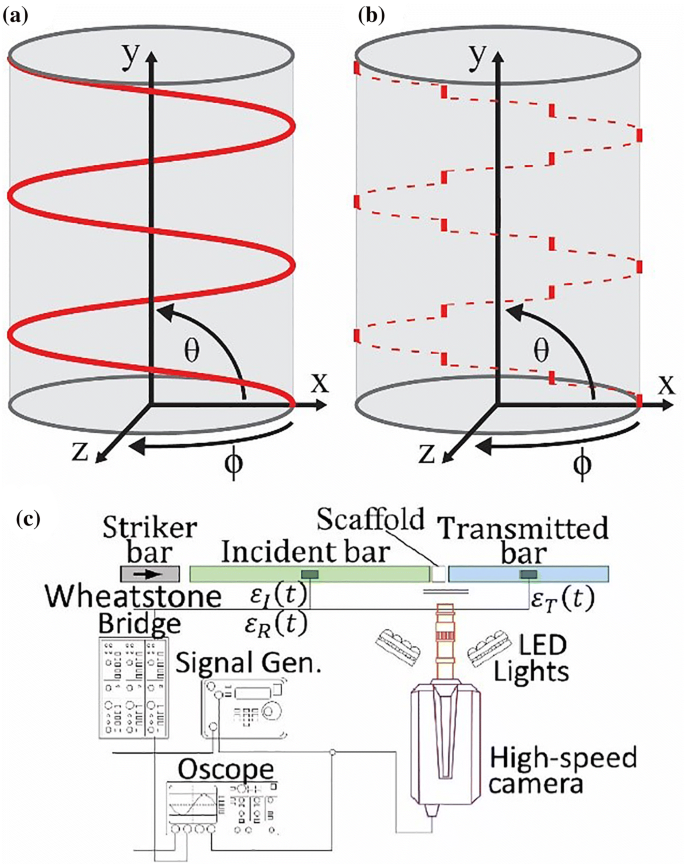
(a) The helical and (b) Bouligand motions of the applied magnetic field. (c) Diagram of the split-Hopkinson pressure bar setup

With θ-direction equal to 0° (group two).
With θ-direction equal to 45° (group three).
Bouligand motions: The freezing slurry was subjected to a magnetic field of 7.8 mT starting in the ϕ = 0° direction, then rotating ϕ by 60° every 1 min, as shown in Fig. 2b.
With θ-direction equal to 0° (group four).
With θ-direction equal to 45° (group five).
The rates of rotation for the helical structures were chosen to have at least one complete magnetic field rotation in the lamellar region of the scaffold. For the Bouligand structures, a rotation (ϕ) of 60° was chosen. This angle was chosen based on empirical observations because it allowed for the lamellar wall angles to produce observable interfaces at the locations where the magnetic field rotates, which made it straightforward to differentiate from the helical structure. Note that, in natural materials, Bouligand structures can have a more gradual rotation between layers than what is demonstrated here. However, to have a contrast with the helical motion tested here, the Bouilgand structure was realized with abrupt transitions between layers. As the tri-axial nested Helmholtz coils are capable of applying a magnetic field in any direction, a y-axis component was also applied to orient the magnetic field at an angle, θ, from the x–z plane. The angle θ of 0° was chosen due to previous reports on lamellar wall alignment when a magnetic field is applied perpendicular to the ice-growth direction.22,31,32 The angle θ of 45° was chosen to mimic the herringbone pattern observed in the impact region of the club of mantis shrimp, which is considered to further increase its impact resistance.33
Following the freezing process, the slurries were lyophilized at 0.047 mBar and -51 °C for 72 h in a Labconco FreeZone 1 freeze drier (Kansas City, MO, USA) to sublimate the grown ice crystals. The green bodies were then sintered at 1150°C for 20 min, with a heating and cooling rate of 2°C/min in an open-air Keith KSK-12 1700 furnace (Pico Rivera, CA, USA). As a result of the sintering process, the Fe3O4 particles experience a phase change to α-Fe2O3 particles.22
Microstructural Characterization
The scaffold microstructures were imaged using an FEI Quanta 600 FG (Hillsboro, Oregon, USA) scanning electron microscope (SEM). SEM images in the x–z plane (perpendicular to the ice growth) at an acceleration voltage of 5 kV and spot size of 2 nm were taken to measure the porosity and pore area. For each image, measurements of the porosity and pore area were made using ImageJ software (National Institutes of Health, Bethesda, MD, USA) by adjusting the threshold to identify porosity, similar to methods used in previous studies.20,32
The lamellar wall directions were measured similar to previous reported methods.22 Two x–z cross section surfaces for each scaffold were SEM imaged. The direction of the magnetic field for each imaged surface was determined by measuring the location along the y-axis and using x–y cross-sectional optical images (Keyence VHX-5000) and relating this to the known magnetic field motion that was applied to the scaffold. To measure the areas and directions of the lamellar walls, the percent areas of lamellar walls aligned were categorized into one of three ranges of angles. Since the magnetic field direction was dynamic throughout the scaffold, the magnetic field direction was defined at 0° and the ranges were defined as: −60° ± 30°, 0° ± 30°, and 60° ± 30°. The closer to 0°, the closer the lamellar walls were to matching the direction of the magnetic field at that location in the scaffold.
Three-dimensional imaging using helical cone-beam micro x-ray computed tomography (µXCT) was conducted on nominally 3 mm diameter and 5 mm tall specimens that were cut out of the center of a specimen from each type of scaffold group. Prior to cutting the scaffolds into these dimensions, they were vacuum infiltrated with EpoxiCure two-part epoxy resin (Buehler, Lake Bluff, IL, USA) then cured for 24 h in ambient air to ensure that the samples could be cut and imaged without altering the internal structure. The epoxy infiltration was done only for handling purposes for the µXCT experiments and not for any other experiments in this research. The µXCT imaging was performed at the Tyree x-ray facilities at the University of New South Wales using the HeliScan™ µXCT. The system has a Hamamatsu x-ray tube with a diamond window, a high-quality flatbed detector (3072 × 3072 pixels, 3.75 fps readout rate) and a helical scanning system. The samples were scanned in a helical trajectory with the following settings: 80 kV x-ray source, 93 µA target current, 0.43 s exposure time, 4 accumulations, 2520 projections per revolution, and 1 mm Al filter. The voxel size obtained was 1.67 µm. The tomographic reconstruction was performed using QMango software developed by the Australian National University. Additional information on helical cone-beam µXCT scanning and reconstruction methods is available.34 Dragonfly software by ORS, Inc. (Montreal, Quebec, Canada) was used to visualize 3D images from the micro-CT scan by stacking layers in the scaffold regions of interest (i.e., where the magnetic field changes directions).
Ice-Growth Velocity
The ice-growth velocity was calculated to observe whether the angle θ of the applied magnetic field and, therefore, the particle alignment, affected the ice-growth velocity. It has been reported that the ice growth velocity directly affects the porosity of freeze cast scaffolds.34,35 Therefore, it was critical to understand whether having a magnetic field with a component in the y-direction (the direction of ice growth) would influence the ice growth velocity and potentially influence the freeze-cast scaffolds beyond the influence of magnetic manipulation. This was done by cutting, then optically imaging, the x–y cross section (parallel to the direction of ice growth) of Bouligand scaffolds fabricated both with θ = 0° and θ = 45°. Bouligand scaffolds were chosen as they had distinct and visible transitions due to the step rotation of the magnetic field. With these images, measurements of the distance between the visible locations where the magnetic field rotated at the center of the scaffolds were made using ImageJ. These distances were then divided by the known time between the rotations the magnetic field (i.e., 1 min) to determine the ice-growth velocity through each region of the magnetic field direction. Of note, since the measurements were taken after the sintering process (i.e., particle densification), this method of obtaining the ice-growth velocity is not the true ice-growth velocity (i.e., during freezing) but provides a way to make comparisons across the Bouligand magnetic field motion scaffolds fabricated in this study with only the applied angle θ acting as a variable.
Quasi-Static Mechanical Characterization
For each scaffold, four quarter-circle shaped specimens where the initial heights were approximately 6 mm and the cross-sectional areas were approximately 50 mm2 were cut from the midsection (i.e., homogenous lamellar ice-growth region36,37) to perform compression tests. The specimens were compressed in the y-direction using an Instron 5967 load frame with an Instron 30-kN load cell (Norwood, MA, USA) at a controlled crosshead speed of 1 mm/min. This resulted in 20 compression tests for each magnetic field motion described in "Sample Preparation" section. The ultimate compressive strength (UCS) was recorded as the maximum engineering compression stress, and the elastic modulus (E) was recorded as the slope of the linear elastic region observed in the stress–strain curve. The strain was recorded as the compressive engineering strain measured from the crosshead displacement.
High Strain Rate Mechanical Characterization
Freeze-cast scaffolds were tested in dynamic compression using a modified split-Hopkinson pressure bar (SHPB). In SHPB experiments (Fig. 2c), a gas gun launches a striker bar towards a coaxially aligned system consisting of a 2.4-m-long incident bar, the freeze-cast scaffold, and a 2.4-m-long transmitted bar. Upon impact of the striker bar with the incident bar, a stress wave is generated that propagates down the length of the incident bar toward the scaffold. At each of the bar-scaffold interfaces, the stress wave is partially reflected backwards, and partially transmitted through the interface. Strain gauges mounted on both the incident and transmission bars sense the elastic deformation of the bars caused by three principal stress waves that pass them: (1) the wave that was caused by the impact of the striker on the incident bar, (2) the wave that was reflected off the incident bar-scaffold interface and back past the strain gauges, and (3) the wave that was transmitted through the scaffold and into the transmission bar. These are the incident, reflected, and transmitted waves, respectively.
Scaffold dimensions were selected such that trade-offs were made between the optimized length to diameter ratios to achieve dynamic stress equilibrium, limit inertia effects, minimize frictional effects, and study a representative volume size. As a result, a total of five scaffolds for each magnetic field motion and 0 mT were tested with thicknesses of approximately 7.5 mm and compression areas of approximately 185 mm2. A reduced initial acceleration was also desirable for the low strength scaffolds to achieve stress equilibrium before failure. A loading pulse with an extended rise time was used to satisfy these experimental requirements. To achieve such a pulse, as well as to eliminate wave dispersion effects, lead pulse shapers 12.7 mm in diameter and 1.58 mm thick were placed at the impacted end of the incident bar. The lead pulse shaper increased the rise time of the loading pulse allowing for the dynamic equilibrium requirement to be met.38 Vacuum grease was also used at the scaffold interfaces to minimize friction effects on the measured mechanical behavior.
The scaffolds were treated as a specialized class of foams, which were considered to be porous soft materials having common characteristics of low strength, stiffness, and low mechanical impedance. To accommodate these materials a hollow transmitted bar was used (see the supplementary information for additional details). The low wave speed of these structures made achieving stress equilibrium challenging despite the use of best practices for soft low impedance materials. To ensure that the strain at failure measurements were valid, high speed imaging of the scaffold deformation was conducted at frame rates of at least 200,000 fps during each experiment. From the image sets captured, the engineering strain of each frame was measured up to the formation of the initial crack and recorded as the compressive strain at failure. The initial crack was defined as the first visible crack that was observed in the high-speed imaging. In addition, the angle of the initial crack was measured using ImageJ. This initial crack angle was defined as the angle from the direction of compression (i.e., y-direction, which also corresponded to the direction of ice growth).
Statistical Analysis
For the measured properties of UCS, E, porosity, and pore area, a one-way analysis of variance (ANOVA) was performed using MATLAB software (Natick, MA, USA) based on the fixed-treatment factor magnetic field motion and a significance level of α = 0.05. If the one-way ANOVA result found that there was a statistically significant difference, this meant that there was a high probability (≥ 95%) that the properties were affected by the magnetic field motion. Following the ANOVA test, a Tukey’s honest significant difference (HSD) test was performed (α = 0.05). This test makes a pairwise comparison across each direction of the magnetic field to pinpoint which scaffolds displayed statistically significant differences from each other. This statistical method has been used previously in freeze-cast research.6,16 For the measured property of strain at initial failure and angle of the initial crack, both measured from the high strain rate tests, the same analyses were performed with α = 0.10. Note that this higher value of α was used due to the inherent variability of high strain rate tests.
Results and Discussion
The microstructural properties of porosity and pore area are shown in Table I. An example of the differing microstructures observed are shown in x–z cross-sections in Fig. 3b and c where the scaffolds were fabricated with a helical magnetic field motion of θ = 0° (where the diagram in Fig. 3a demonstrates the angle ranges that were measured in this study, with the angle of 0° set at the applied magnetic field direction for the scaffold shown in Fig. 3b) and 0 mT, respectively. Applying the magnetic field motions resulted in a decrease of the x–z cross-section porosity by up to 42%. Decreases in porosity when applying a magnetic field have been previously reported.21 Additionally, the mean pore area decreased as a result of the magnetic field motions. Because the Fe3O4 particles chain together and align in the magnetic field direction during freezing, this alters the interactions between the progressing ice front and the chained particles, thus altering the porosity and pore area.22

(a) The magnetic field direction (0°) of (b) where the scaffold was fabricated with a helical magnetic field motion θ of 0°. (c) The surface of a scaffold fabricated with 0 mT. The percent area of lamellar walls aligned in the range of angles of −60° ± 30°, 0° ± 30°, and 60° ± 30° for scaffolds fabricated with (d) 0 mT, helical magnetic field motions with θ of (e) 0°, and (f) 45°; and Bouligand magnetic field motions with θ of (g) 0° and (h) 45°. The values shown are the means ± one standard deviation (n = 10). The scale bar are 200 μm. Properties observed to have statistically significant differences (p ≤ 0.05) are noted by nonmatching letters a-b
When no magnetic field was applied, the distribution of the lamellar wall directions was evenly distributed as shown in Fig. 3d. When a magnetic field was applied, the majority (53–67%) of the lamellar walls aligned within ± 30° of the magnetic field (0°) direction as shown in Fig. 3e–h, with the minority (33–47%) of the lamellar walls aligned in angle ranges furthest from the magnetic field direction (i.e., −60° ± 30° and 60° ± 30°). The one-way ANOVAs for Fig. 3e–h were 0.1532, 0.004, 0.0008, and 0.0013, respectively, resulting in statistically significant differences in all cases except that with a helical magnetic field motion of θ = 0°. Pairwise statistically significant differences using Tukey’s HSD tests were observed between the 0° ± 30° range and both the −60° ± 30° and 60° ± 30° ranges for the helical magnetic field motion with θ of 45° (Fig. 3f) and the Bouligand magnetic field motions with θ of 0° (Fig. 3g) and 45° (Fig. 3h). As previously reported,22,31,32 lamellar walls tended to align in the magnetic field direction due to chaining and alignment prior to being segregated by the growing ice crystals during the freezing processes.
While a statistically significant difference in the lamellar wall alignment when three of the magnetic field motions were applied (Fig. 3f–h) was found, the % area aligned with the magnetic field was lower than a previous report, using similar techniques but a static field, of up to 84% area within ± 22.5° of the magnetic field direction22. This was hypothesized to be due to the dynamic application of the magnetic field during the freezing process, thus resulting in less time for the particles to chain together and align. Additionally, it has been reported that even when the lamellar walls do not align with the magnetic field, mineral bridges can become longer, thicker, and aligned with the magnetic field direction, also resulting in a decrease in porosity,19 as was observed in this report.
Differences between x–y cross sections of scaffolds fabricated in each magnetic field motion are shown in Fig. 4. It was observed that when no magnetic field is applied (Fig. 4a), areas of random pore direction (i.e., no lamellar wall alignment) were seen throughout the scaffold. This is a typical feature of freeze-cast scaffolds.22 In the helical motion scaffolds, darker and lighter bands were observed parallel to the x-direction and perpendicular to the y-direction (Fig. 4b and c). These bands were due to the lamellar walls being aligned in the rotating direction of the magnetic field and were optically visible due to the changing proportion of the lamellar walls being aligned with the imaged cross section. Because the pores are elliptical cylinders, the lighter regions were caused by the lamellar walls being aligned predominantly in the ϕ = 0° or 180° direction where the wider faces of the lamellar walls are visible. Similarly, the darker regions were from the lamellar walls being predominantly in the ϕ = 90° or 270° direction where the shorter faces of the lamellar walls were visible. In the Bouligand motion scaffolds, darker and lighter bands were also observed parallel to the x-direction and perpendicular to the y-direction (Fig. 4d and e, along with a magnified SEM image of the interface in Fig. 4f). These regions were more visible than the helical motion scaffolds as the magnetic field flips instantly by ϕ = 60° every 1 min, making the light and dark region interface transition instantly as opposed to gradually. Note that a single flip, though not a dynamic process, in the magnetic field has previously been reported with a similarly observed interface.22 These regions of variable pore directions were also observed, using a micro-CT scan, to occur throughout the scaffolds, as shown in Fig. 5. Similar to the optical images, there are distinct locations along the y-direction where the microstructure varies depending on the magnetic field direction. The locations of these changes in microstructure are shown by black lines drawn across the images in the x-direction.

Example optical images of x–y plane cross sections of (a) a scaffold fabricated using no magnetic field (0 mT), helical magnetic field motions with θ of (b) 0°, and (c) 45°; and Bouligand magnetic field motions with θ of (d) 0° and (e) 45° along with an enlarged area (f) imaged using SEM. The arrows in (b) and (c) show the locations of specific values of ϕ. The arrows in (d) and (e) show the observable locations of ϕ values. The scale bars of (a–e) are 2 mm and of (f) is 0.5 mm

Processed images from a micro-CT scan of (a) a scaffold fabricated using no magnetic field (0 mT), helical magnetic field motions with θ of (b) 0° and (c) 45°, and Bouligand magnetic field motions with θ of (d) 0° and (e) 45°. The scale bars are 100 μm
The measured ice-growth velocities using a post hoc technique along the y-direction of each region of ϕ is shown in Fig. 6. The velocity measurements were all made above the dense region and in the lamellar region as indicated in Fig. 6a. It was observed that the mean velocity was 1.32 mm/min for a θ of 0° type Bouligand magnetic field motion (Fig. 6b) and 1.33 mm/min for a θ of 45° type motion (Fig. 6c). As a result, the mean ice-growth velocity did not experience any statistically significant changes throughout the freezing process as a result of the magnetic field direction. Of note, these velocities are of similar magnitudes to previously reported ice-growth velocities of 2.27 mm/min39 and are lower due to the post hoc nature of the test, where the sintering process has densified the material. This method of measuring ice-growth velocity was only possible with the Bouligand magnetic field motion scaffolds because the interfaces at the locations of changing ϕ were clearly visible both optically (Figs. 4d, e and 6a) and with SEM (Fig. 4f). Note that this technique for measuring the ice-growth velocity could be used to make measurements on future fabricated scaffolds by making magnetic field motions that can be similarly identified (Fig. 6a).

(a) An example x–y cross-section optical image of a scaffold fabricated under a Bouligand magnetic field motion indicating the magnetic field ϕ component perpendicular to the y-direction. The lengths of each ϕ-region perpendicular to the y-direction, when combined with the known time between ϕ-regions (i.e., 1 min) correspond to the ice-growth velocity of the Bouligand magnetic field motion scaffolds fabricated with magnetic field θ of (b) 0° and (c) 45°. The values shown are the means ± one standard deviation (n = 5). The scale bars is 2 mm
The images observed by the high-speed camera during SHPB testing (Fig. 7a–e) and resultant crack angles (Fig. 7f) showed that the crack paths were dependent on the application of a magnetic field (ANOVA, p = 0.0002). When the scaffolds were fabricated with no magnetic field, cracks followed the y-direction of compression (i.e., 0°) as shown in Fig. 7a. When the scaffolds were fabricated with magnetic field motion, cracks grew at an angle away from the direction of compression. This is shown in Figs. 7b–e where cracks tended to propagate at an angle much higher than 0°. Of particular note, in the cases of a helical magnetic field motion with a θ of 0° and the Bouilgand magnetic field with a θ of 45°, the mean crack angles were 66° and 61°, respectively (Fig. 7f). These angles closely followed the applied rotating angle of the magnetic field of 71° and 67°, respectively. This suggested that the crack path was controlled by the direction of the magnetic field motion during fabrication, thus providing control over the fracture properties. The cracks that formed during quasi-static loading followed a similar trajectory, with those occurring in scaffolds fabricated with no magnetic field following the y-direction of compression and those scaffolds fabricated with a magnetic field occurring away from the y-direction of compression.

Example images of SHPB compression tests in the y-direction, with the initial crack highlighted, for scaffolds fabricated under (a) 0 mT, helical magnetic field motions with θ of (b) 0° and (c) 45°, and Bouligand magnetic field motions with θ of (d) 0° and (e) 45°. (f) The initial failure crack angle of each magnetic field motion type. (g) The strain at initial failure for each type of magnetic field motion scaffold using the SPHB for high strain rate compression tests. The values shown are the means ± one standard deviation (n = 5). (h) Representative stress–strain curves for SHPB experiments. (i) Representative stress–strain curves for quasi-static experiments. The scale bars are 4 mm. Properties observed to have statistically significant differences (p ≤ 0.10) are noted by nonmatching letters (f) a–d and (g) y and z
For the SHPB experiments, the strain at the point of initial failure (i.e., an observed crack with the high-speed camera) increased when applying a magnetic field motion compared to no magnetic field, as shown in Fig. 7g. Note that the ANOVA (with α = 0.10) resulted in p = 0.0546. The scaffolds were therefore more resilient to catastrophic failure. This was similar to what is seen in nature for helical and Bouligand structures in the dactyl club of mantic shrimp and the exoskeleton of grasshoppers, which resist failure from impacts when hunting prey and resisting predation, respectively.4,40,41,42,–43 An increase of as much as 212% occurred between applying 0 mT and a helical magnetic field motion with θ of 45° (p = 0.0624). The motions with θ of 45° were observed to have a higher mean than motions with θ of 0° suggesting that the y-component of the magnetic field could be assisting in delaying the failure from high strain rate compression. The maximum stress and energy absorbed before failure from the SHPB experiments (Table I) showed no statistically significant differences when tested with an ANOVA analysis (p = 0.5518 and p = 0.2027 for the maximum stress and energy absorbed before failure, respectively), though an increase in the energy absorbed before failure was observed with the applied magnetic fields. In addition, representative stress–strain curves are presented in Fig. 7h and i, which display the increased strain at failure of the SHPB experiments with an applied magnetic field.
In contrast to the SHPB experiments, quasi-static compression tests showed no statistically significant differences in the UCS and E as a function of applied magnetic field motion and 0 mT (Table I). When considered with the control of the crack trajectory and increase in the energy absorbance, this technique allowed for an increase in the high strain rate mechanical properties without impacting the quasi-static mechanical properties. Note that a decrease in the porosity and pore area often results in an increase in the quasi-static UCS and E.15,44 This, however, is not always the case as similar particles and freezing parameters have yielded similar results,22 and was likely due to the dynamic nature of the applied magnetic field employed here. Previous work on high strain rate compression tests on freeze-cast composite and ceramic materials also showed a drastic enhancement of the dynamic mechanical properties compared to quasi-static properties as a result of the freezing rate45 and solid loading particle concentration.46
With the tri-axial nested Helmholtz coils-based freeze-casting setup that was used in this study, the microstructure at specific locations in scaffolds was customized by controlling the magnetic field as the slurry was freezing. This was made possible because the uniformity of the magnetic field generated by the Helmholtz coils created homogenous structures (i.e., the particles did not agglomerate).21 This was unique in that it created a uniform magnetic field in any direction compared to previous permanent magnet setups where multiple setups had to be made to apply magnetic fields in desired directions and motions.18,19 This work has advanced the ability to customize the properties of porous scaffolds through magnetic freeze casting user-specific properties at user-specific locations. With the ability to control the magnetic field, more magnetic field motions could be investigated furthering the improvements of the mechanical properties in bioinspired materials.
Conclusion
This study of fabricating bioinspired helical and Bouligand structures through magnetic freeze casting using tri-axial nested Helmholtz coils enabled the following conclusions:
The microstructure properties changed as a result of applying the magnetic field motions. The porosity and pore area decreased by as much as 42% and 20%, respectively, from applying no magnetic field (0 mT).
The ice-growth velocity was observed through a novel technique showing that the ice-growth velocity stayed consistent throughout the scaffold freezing regardless of the applied magnetic field direction of θ (in the direction of ice growth).
Impact testing revealed that the dynamic crack growth directions were altered by applying a magnetic field in helical and Bouligand motions. In the cases of helical motion with a θ of 0° and Bouligand motion of θ of 45°, the dynamic crack paths closely followed the rotation path of the magnetic field.
Scaffolds fabricated with a magnetic field motion showed higher dynamic impact strains before initial failure compared to the case of no magnetic field in impact loading.
The impact resistance properties of these bioinspired materials increased due to the effect of the magnetic field motions without affecting the quasi-static mechanical properties.
References
S.E. Naleway, M.M. Porter, J. McKittrick, and M.A. Meyers, Adv. Mater. 27, 5455–5476 (2015).
M.E. Launey, M.J. Buehler, and R.O. Ritchie, Annu. Rev. Mater. Res. 40, 25–53 (2010).
N. Suksangpanya, N.A. Yaraghi, D. Kisailus, and P. Zavattieri, J. Mech. Behav. Biomed. Mater. 76, 38–57 (2017).
J.C. Weaver, G.W. Milliron, A. Miserez, K. Evans-Lutterodt, S. Herrera, I. Gallana, W.J. Mershon, B. Swanson, P. Zavattieri, E. DiMasi, and D. Kisailus, Science 336, 1275–1280 (2012).
Y. Zhang, J. Roscow, M. Xie, and C. Bowen, J. Eur. Ceram. Soc. 38, 4203–4211 (2018).
T.A. Ogden, M. Prisbrey, I. Nelson, B. Raeymaekers, and S.E. Naleway, Mater. Des. 164, 107561 (2018).
M. Naviroj, P.W. Voorhees, and K.T. Faber, J. Mater. Res. 32, 3372 (2017).
Y. Chino and D.C. Dunand, Acta Mater. 56, 105 (2008).
H.D. Jung, S.W. Yook, T.S. Jang, Y. Li, H.E. Kim, and Y.H. Koh, Mater. Sci. Eng. C Mater. Biol. Appl. 33, 340–346 (2013).
H.-D. Jung, S.-W. Yook, H.-E. Kim, and Y.-H. Koh, Mater. Lett. 63, 1545 (2009).
H. Schoof, J. Apel, I. Heschel, and G. Rau, J. Biomed. Mater. Res. 58, 352–357 (2001).
H.W. Kang, Y. Tabata, and Y. Ikada, Biomaterials 20, 1339–1344 (1999).
T. Kohnke, T. Elder, H. Theliander, and A.J. Ragauskas, Carbohydr. Polym. 100, 24–30 (2014).
S. Roy and A. Wanner, Compos. Sci. Technol. 68, 1136 (2008).
P.M. Hunger, A.E. Donius, and U.G. Wegst, Acta Biomater. 9, 6338–6348 (2013).
S.E. Naleway, K.C. Fickas, Y.N. Maker, M.A. Meyers, and J. McKittrick, Mater. Sci. Eng. C Mater. Biol. Appl. 61, 105–112 (2016).
A. Shaga, P. Shen, C. Sun, and Q. Jiang, Mater. Sci. Eng. A 630, 78 (2015).
M.M. Porter, L. Meraz, A. Calderon, H. Choi, A. Chouhan, L. Wang, M.A. Meyers, and J. McKittrick, Compos. Struct. 119, 174–184 (2015).
M.M. Porter, P. Niksiar, J. McKittrick, and G. Franks, J. Am. Ceram. Soc. 99, 1917–1926 (2016).
M.M. Porter, M. Yeh, J. Strawson, T. Goehring, S. Lujan, P. Siripasopsotorn, M.A. Meyers, and J. McKittrick, Mater. Sci. Eng. A 556, 741–750 (2012).
I. Nelson, T.A. Ogden, S. Al Khateeb, J. Graser, T.D. Sparks, J.J. Abbott, and S.E. Naleway, Adv. Eng. Mater. 21, 1801092 (2019).
I. Nelson, L. Gardner, K. Carlson, and S.E. Naleway, Acta Mater. 173, 106 (2019).
J.P. Randall, M.A. Meador, and S.C. Jana, ACS Appl. Mater. Interfaces 3, 613–626 (2011).
N.P. Padture, Nat. Mater. 15, 804–809 (2016).
K.S. Katti, Colloids Surf. B Biointerfaces 39, 133–142 (2004).
J. Currey, J. Theor. Biol. 231, 569–580 (2004).
J.D. Currey, Calcif. Tissue Int. 36, 118–122 (1984).
J.J. Abbott, Rev. Sci. Instrum. 86, 124902 (2015).
A.M.A. Silva, E.H.M. Nunes, D.F. Souza, D.L. Martens, J.C. Diniz da Costa, M. Houmard, and W.L. Vasconcelos, Ceram. Int. 41, 10467–10475 (2015).
D.F. Souza, E.H.M. Nunes, D.S. Pimenta, D.C.L. Vasconcelos, J.F. Nascimento, W. Grava, M. Houmard, and W.L. Vasconcelos, Mater. Charact. 96, 183–195 (2014).
M.B. Frank, S.H. Siu, K. Karandikar, C.H. Liu, S.E. Naleway, M.M. Porter, O.A. Graeve, and J. McKittrick, J. Mech. Behav. Biomed. Mater. 76, 153–163 (2017).
M.B. Frank, S.E. Naleway, T. Haroush, C.-H. Liu, S.H. Siu, J. Ng, I. Torres, A. Ismail, K. Karandikar, M.M. Porter, O.A. Graeve, and J. McKittrick, Mater. Sci. Eng. C 77, 484–492 (2017).
N.A. Yaraghi, N. Guarin-Zapata, L.K. Grunenfelder, E. Hintsala, S. Bhowmick, J.M. Hiller, M. Betts, E.L. Principe, J.Y. Jung, L. Sheppard, R. Wuhrer, J. McKittrick, P.D. Zavattieri, and D. Kisailus, Adv. Mater. 28, 6835–6844 (2016).
S. Deville, E. Saiz, and A.P. Tomsia, Acta Mater. 55, 1965–1974 (2007).
U.G. Wegst, M. Schecter, A.E. Donius, and P.M. Hunger, Philos. Trans. A Math. Phys. Eng. Sci. 368, 2099–2121 (2010).
S. Deville, J. Mater. Res. 28, 2202–2219 (2013).
S. Deville, E. Maire, A. Lasalle, A. Bogner, C. Gauthier, J. Leloup, and C. Guizard, J. Am. Ceram. Soc. 93, 2507–2510 (2010).
G. Ravichandran and G. Subhash, J. Am. Ceram. Soc. 77, 263–267 (1994).
S. Deville, E. Maire, A. Lasalle, A. Bogner, C. Gauthier, J. Leloup, and C. Guizard, J. Am. Ceram. Soc. 92, 2497 (2009).
S. Amini, M. Tadayon, S. Idapalapati, and A. Miserez, Nat. Mater. 14, 943 (2015).
Y. Bouligand, Tissue Cell 4, 189–217 (1972).
L.K. Grunenfelder, N. Suksangpanya, C. Salinas, G. Milliron, N. Yaraghi, S. Herrera, K. Evans-Lutterodt, S.R. Nutt, P. Zavattieri, and D. Kisailus, Acta Biomater. 10, 3997–4008 (2014).
N. Suksangpanya, N.A. Yaraghi, R.B. Pipes, D. Kisailus, and P. Zavattieri, Int. J. Solids Struct. 150, 83 (2018).
M.M. Porter, R. Imperio, M. Wen, M.A. Meyers, and J. McKittrick, Adv. Funct. Mater. 24, 1978–1987 (2014).
S. Akurati, N. Tennant, and D. Ghosh, J. Mater. Res. 34, 959 (2019).
M. Banda and D. Ghosh, Acta Mater. 149, 179 (2018).
Acknowledgements
This work was financially supported in part by the National Science Foundation under Grant CMMI #1660979. The authors further acknowledge the Tyree x-ray CT Facility, a UNSW network lab funded by the UNSW Research Infrastructure Scheme, for the acquisition of the 3D µXCT images.
Author information
Authors and Affiliations
Corresponding author
Additional information
Publisher's Note
Springer Nature remains neutral with regard to jurisdictional claims in published maps and institutional affiliations.
Electronic supplementary material
Below is the link to the electronic supplementary material.
Rights and permissions
About this article

Cite this article
Nelson, I., Varga, J., Wadsworth, P. et al. Helical and Bouligand Porous Scaffolds Fabricated by Dynamic Low Strength Magnetic Field Freeze Casting. JOM 72, 1498–1508 (2020). https://doi.org/10.1007/s11837-019-04002-9
Received:
Accepted:
Published:
Issue Date:
DOI: https://doi.org/10.1007/s11837-019-04002-9