Using Semicontinuity for Standard Bases Computations

Abstract

We present new results on standard basis computations of a 0-dimensional ideal I in a power series ring or in the localization of a polynomial ring over a computable field K. We prove the semicontinuity of the “highest corner” in a family of ideals, parametrized by the spectrum of a Noetherian domain A. This semicontinuity is used to design a new modular algorithm for computing a standard basis of I if K is the quotient field of A. It uses the computation over the residue field of a “good” prime ideal of A to truncate high order terms in the subsequent computation over K. We prove that almost all prime ideals are good, so a random choice is very likely to be good, and whether it is good is detected a posteriori by the algorithm. The algorithm yields a significant speed advantage over the non-modular version and works for arbitrary Noetherian domains. The most important special cases are perhaps $A={\mathbb {Z}}$ and $A=k[t]$, k any field and t a set of parameters. Besides its generality, the method differs substantially from previously known modular algorithms for $A={\mathbb {Z}}$, since it does not manipulate the coefficients. It is also usually faster and can be combined with other modular methods for computations in local rings. The algorithm is implemented in the computer algebra system Singular and we present several examples illustrating its power.

1 Introduction

When studying numerical invariants of singularities of an algebraic variety X at a point one is often led at some point to compute the dimension $\dim _{K}K[x]_{\langle x \rangle }/I$ for some field K and I an ideal in K[x]. Typical examples are the Milnor number or the Tjurina number of an isolated hypersurface singularity, but also many others. These computations are usually done by computing a standard basis of I. Due to intermediate coefficient growth this can be very time and space consuming for $K={\mathbb {Q}}$ or $K=k(t)$, the quotient field of k[t] for some field k and finitely many parameters $t=(t_1,\ldots ,t_s)$.

In the present paper we provide a modular version of an algorithm for the computation of $\dim _K K[x]_{\langle x \rangle }/I=\dim _{K}K[[x]]/I$ (which we assume to be finite), where $K= {{\,\textrm{Quot}\,}}(A)$ is the quotient field of a Noetherian integral domain A. Let $\mathfrak {p}$ be a prime ideal in A and $k(\mathfrak {p})$ its residue field. We use a modular computation over $k(\mathfrak {p})$ and then use the bound given by the highest corner of the modular computation to cut off high order terms from the polynomials during the subsequent standard basis computation over K. To simplify notation we set

$$\begin{aligned} R(0):=K[x]_{\langle x \rangle }\text { and } R(\mathfrak {p}):=k(\mathfrak {p})[x]_{\langle x \rangle }. \end{aligned}$$

We start the algorithm (Algorithm 5.2) by choosing an arbitrary prime ideal $\mathfrak {p}\ne \langle 0\rangle$ and compute a standard basis of the induced ideal $I(\mathfrak {p})$, the image under the natural map $A[x] \rightarrow R(\mathfrak {p})$. The computation decides if $\mathfrak {p}$ is “half-good”, i.e.,

$$\begin{aligned} \dim _{k(\mathfrak {p})} R(\mathfrak {p})/I(\mathfrak {p}) <\infty . \end{aligned}$$

Then the ideal $I(\mathfrak {p})$ has a so called “highest corner” $HC(I(\mathfrak {p}))$, introduced in [4], which is the smallest monomial (w.r.t. to the local monomial order) not contained in the leading ideal $L(I(\mathfrak {p}))$. $HC(I(\mathfrak {p}))$ can be read from the leading terms of the standard basis of $I(\mathfrak {p})$. We then compute a standard basis of the ideal $I(0)=IR(0)$ over K, but during the computation we cut off high order terms from the involved polynomials.

The bound for cutting off is deduced from $HC(I(\mathfrak {p}))$ (Theorem 4.2). The result is a standard basis of an ideal $I'(0) \supset I(0)$, which is equal to I(0) if $\dim _{k(\mathfrak {p})}R(\mathfrak {p})/I(\mathfrak {p}) = \dim _{k(0)}R(0)/I'(0)$ (Proposition 3.5). If this is the case we say that $\mathfrak {p}$ is ”good” and a standard basis of I(0) has been computed (if $\mathfrak {p}$ is not half-good, we restart the algorithm with another choice of $\mathfrak {p}$).

To prove correctness of the algorithm, i.e., that the result is in fact a standard basis of I(0), we will prove that the highest corner is lower semicontinuous in the Zariski topology of ${{\,\textrm{Spec}\,}}A$ (Proposition 3.5). This is in turn deduced from a general semicontinuity theorem in [5] (see Theorem 3.1). An important fact is that half-good and good prime ideals form a open dense subset of ${{\,\textrm{Spec}\,}}A$ if A contains infinitely many prime ideals (Theorem 5.2), so that the algorithm terminates for a “sufficiently general” choice of $\mathfrak {p}$. We remark that just one sufficiently general $\mathfrak {p}$ suffices. For A a principal ideal domain, only finitely many prime ideals are bad, so that the algorithm terminates always after finitely many steps for any choice of $\mathfrak {p}$ (Corollary 5.4). After each run the algorithm shows whether the chosen prime ideal was good or bad.

In Sect. 5 we illustrate the results for the special cases $A={\mathbb {Z}}$ (with $K={\mathbb {Q}}$ and $k(\mathfrak {p})={\mathbb {F}}_p$, p a prime number) and for $A=k[t_1,\ldots ,t_s]$ (with $K=k(t_1,\ldots ,t_s)$ and $k(\mathfrak {p})=k$, $\mathfrak {p}= \langle t_1-p_1,\ldots ,t_s-p_s\rangle$ for some point $(p_1,\ldots ,p_s)\in k^s$) and for these rings we provide non-trivial examples in Sect. 6 that demonstrate the impressive speed up over the non-modular algorithms. The examples show also that Algorithm 5.2 is often faster than previously known modular methods for $A={\mathbb {Z}}$. The high performance of the algorithm is due to the reduction of the number of terms of the polynomials involved (and not to the avoidance of coefficient growth when $A={\mathbb {Z}}$) and thus it can be combined with previous modular algorithms.

The computations are done in the computer algebra system Singular [3] and the examples show how this can be done in general with a few Singular-commands.¹

While our algorithm is of course based on the standard basis theory for non-well orderings developed in [4], the main new ingredient is the semicontinuity theorem in [5], a result that has nothing to do with any computational aspects. It is used to prove both correctness and termination of Algorithm 5.1, but the proofs are by no means obvious. The main new theoretical results are Proposition 3.5, Theorems 4.2, and 5.2. Algorithm 5.1 not only provides (in the local case) a new modular method for $A={\mathbb {Z}}$, it is also valid for a general Noetherian domain A (with computable residue fields) and we are not aware of any modular algorithm that works in this generality.

2 Notation

The following is used throughout the paper. A denotes a Noetherian integral domain, A[x], $x=(x_1,\ldots ,x_n)$, the polynomial ring over A and $I\subset A[x]$ an ideal (the symbols $\subset$, resp. $\supset$, mean $\subseteq$, resp. $\supseteq$, in this paper). For a prime ideal $\mathfrak {p}$ in A let $k(\mathfrak {p}):=A_\mathfrak {p}/\mathfrak {p}A_\mathfrak {p}= {{\,\textrm{Quot}\,}}(A/\mathfrak {p})$ be the residue field of the local ring $A_\mathfrak {p}$. In particular, $k(0):=k(\langle 0\rangle )={{\,\textrm{Quot}\,}}(A)$. The map $A \rightarrow k(\mathfrak {p})$ induces natural maps $A[x] \rightarrow k(\mathfrak {p})[x] \rightarrow k(\mathfrak {p})[x]_{\langle x \rangle }\rightarrow (k(\mathfrak {p})[x]_{\langle x \rangle })^\wedge = k(\mathfrak {p})[[x]]$, with $^\wedge$ the ${\langle x \rangle }$-adic completion. We set

$$\begin{aligned} R(\mathfrak {p}):=k(\mathfrak {p})[x]_{\langle x \rangle }\text { and } {\hat{R}}(\mathfrak {p}):=k(\mathfrak {p})[[x]], \end{aligned}$$

and denote by $I(\mathfrak {p})$ resp. ${\hat{I}}(\mathfrak {p})$ the ideal in $R(\mathfrak {p})$ resp. in ${\hat{R}}(\mathfrak {p})$ generated by the image of I under the above maps. Instead of $R(\langle 0\rangle )$ and $I(\langle 0\rangle )$ we write R(0) and I(0). Note that

$$\begin{aligned} \dim _{k(\mathfrak {p})} R(\mathfrak {p})/I(\mathfrak {p})< \infty \iff \dim _{k(\mathfrak {p})} {\hat{R}}(\mathfrak {p})/{\hat{I}}(\mathfrak {p}) <\infty \end{aligned}$$

and that then the dimensions coincide.

3 Semicontinuity of the Highest Corner

The following semicontinuity theorem is a special case of [5, Theorem 42]. It is the main ingredient for the correctness of our algorithm.

Theorem 3.1

For any fixed $\mathfrak {p}\in {{\,\textrm{Spec}\,}}A$ there is an open neighbourhood U of $\mathfrak {p}$ in ${{\,\textrm{Spec}\,}}A$ such that

$$\begin{aligned} \dim _{k(\mathfrak {q})} {\hat{R}}(\mathfrak {q})/{\hat{I}}(\mathfrak {q}) \le \dim _{k(\mathfrak {p})} {\hat{R}}(\mathfrak {p})/{\hat{I}}(\mathfrak {p}) \text{ for } \text{ all } \mathfrak {q}\in U. \end{aligned}$$

The inequality is of interest only if $\dim _{k(\mathfrak {p})} {\hat{R}}(\mathfrak {p})/{\hat{I}}(\mathfrak {p}) <\infty$ since it holds trivially if $\dim _{k(\mathfrak {p})} {\hat{R}}(\mathfrak {p})/{\hat{I}}(\mathfrak {p}) =\infty$.

Corollary 3.2

For each $N=0,1,2,\ldots ,\infty$ the set

$$\begin{aligned} D_N:=\{\mathfrak {p}\in {{\,\textrm{Spec}\,}}A |\ \dim _{k(\mathfrak {p})} R(\mathfrak {p})/I(\mathfrak {p}) \le N\} \end{aligned}$$

is open in ${{\,\textrm{Spec}\,}}A$ and for each $\mathfrak {p}\in {{\,\textrm{Spec}\,}}A$ we have

$$\begin{aligned} \dim _{k(0)} R(0)/ I(0) \le \dim _{k(\mathfrak {p})} R(\mathfrak {p})/ I(\mathfrak {p}). \end{aligned}$$

Moreover, $\dim _{k(0)} R(0)/ I(0) = \dim _{k(\mathfrak {p})} R(\mathfrak {p})/ I(\mathfrak {p})$ for $\mathfrak {p}$ in an open dense subset of ${{\,\textrm{Spec}\,}}A$.

Proof

Since the prime ideal $\langle 0\rangle$ is contained in every neighbourhood of any prime ideal $\mathfrak {p}$, Theorem 3.1 and the last statement of Sect. 2 imply the openness of $D_N$ and the inequality $\dim _{k(0)} R(0)/ I(0) \le \dim _{k(\mathfrak {p})} R(\mathfrak {p})/ I(\mathfrak {p})$. Taking $\mathfrak {p}= \langle 0\rangle$ in Theorem 3.1 we get the other inequality and hence equality for an open set. If $\dim _{k(0)} R(0)/ I(0) =\infty$, this set is ${{\,\textrm{Spec}\,}}A$ and if $\dim _{k(0)} R(0)/ I(0) <\infty$, this set is non-empty, hence dense since A is an integral domain.

$\square$

We recall now the definition of the highest corner from [4, Definition 1.7.11]. It uses the notion of a local monomial ordering > on a polynomial ring $A[x_1,\ldots ,x_n]$², A any ring.

Definition 3.3

Let K be a field, $I \subset K[x]$ a proper ideal, and > a local monomial ordering on K[x]. A monomial m is called the highest corner of I (with respect to >), denoted by HC(I), if

• 1. $m \notin L(I)$, where $L(I)\subset K[x]$ is the leading ideal ³ of I,

• 2. if $m'$ is a monomial with $m' <m$ $\Longrightarrow m' \in L(I)$.

It shown in [4, Lemma 1.7.13] that HC(I) is the smallest monomial (with respect to >) not contained in I.

In the following we need local weighted degree orderings ⁴, where the variables have negative weights (see [4, Definition 1.2.9]). It is called a local degree ordering if weight$(x_i) = -1$ for each i ⁵, see Fig. 1 for an example.

Fig. 1

$L(\langle y^4\!+x^5,x^3y^3\rangle )$ (for the local degree ordering ds) is generated by the monomials $y^4,x^3y^3,x^8$ (marked by a $\bullet$). The highest corner is $x^7y^2$ (marked by a $\bigstar$)

Lemma 3.4

Let $\mathfrak {p}$ be a fixed prime ideal in A such that $\dim _{k(\mathfrak {p})} R(\mathfrak {p})/ I(\mathfrak {p}) < \infty$ and let > be a local weighted degree ordering on $Mon(x_1,\ldots , x_n)$. Then $HC(I(\mathfrak {q}))$ exists for all $\mathfrak {q}$ in some open neighbourhood of $\mathfrak {p}$ in ${{\,\textrm{Spec}\,}}A$. In particular, HC(I(0)) exist.

Proof

This follows from [4, Lemma 1.7.14] and Corollary 3.2. $\square$

We prove now the semicontinuity of the highest corner.

Proposition 3.5

With the assumptions of Lemma 3.4 let ${\mathcal {M}}$ be a set of monomials m such that $m< HC(I(\mathfrak {p}))$ and set $I'(0):= I(0)+\langle {\mathcal {M}}\rangle _{R(0)}.$

• (i) If $\dim _{k(\mathfrak {p})} R(\mathfrak {p})/ I(\mathfrak {p}) = \dim _{k(0)} R(0)/ I'(0)$ then $I'(0) = I(0)$.

• (ii) If $\dim _{k(\mathfrak {p})} R(\mathfrak {p})/ I(\mathfrak {p}) = \dim _{k(0)} R(0)/ I'(0)$ with ${\mathcal {M}}$ the set of all monomials $< HC(I(\mathfrak {p}))$, then

  $$\begin{aligned} HC(I(0))\ge HC(I(\mathfrak {p})). \end{aligned}$$

Proof

(i) From Corollary 3.2 we get

$$\begin{aligned} \dim _{k(0)} R(0)/I'(0) \le \dim _{k(0)} R(0)/I(0) \le \dim _{k(\mathfrak {p})} R(\mathfrak {p})/I(\mathfrak {p}). \end{aligned}$$

The assumption implies $\dim _{k(0)} R(0)/I'(0) = \dim _{k(0)} R(0)/I(0)$ and hence $I'(0) = I(0)$.

(ii) Now let ${\mathcal {M}}$ be the set of all monomials $< HC(I(\mathfrak {p}))$. Since $I'(0) = I(0)$, $m \in I(0)$ and hence $m \in L(I(0))$ for all $m < HC(I(\mathfrak {p}))$. It follows that $HC(I(0)) \ge HC(I(\mathfrak {p}))$. $\square$

Remark 3.6

Theorem 3.1 is proved in [5] more generally for submodules $I\subset A[x]^m$ with ${\hat{R}}(\mathfrak {q})/{\hat{I}}(\mathfrak {q})$ replaced by ${\hat{R}}(\mathfrak {q})^m/{\hat{I}}(\mathfrak {q})$, such that Corollary 3.2 holds also for modules. The highest corner can be defined in the same way for submodules of $K[x]^m$ and then Lemma 3.4, Proposition 3.5 and Algorithm 5.2 hold analogously for modules (but we do not pursue this here).

4 A Bound for Truncation

Proposition 4.1

Let K be a field, > a local weighted degree ordering on K[x], $I \subset K[x]$ an ideal with $\dim _K K[x]_{\langle x \rangle }/I <\infty$, and $m\le HC(I)$ a monomial. Let $g_1,\ldots ,g_s$ be a minimal standard basis ⁶ of I and $x_{i_0}$ the biggest variable w.r.t. > appearing in $LM(g_i)$. Then

$$\begin{aligned} w\text {-}\deg (LM(g_i)) \ge w\text {-}\deg (m)+w\text {-}\deg (x_{i_0}) \text { for all } i. \end{aligned}$$

In particular, if > is a local degree ordering we have

$$\begin{aligned} \deg (LM(g_i)) \le \deg (m)+1 \text { for all } i. \end{aligned}$$

Proof

Let $(w_1,\ldots ,w_n)$, $w_i<0$, be a weight vector defining >. By definition of HC(I), all monomials $< HC(I)$ are contained in L(I). Since we have a local weighted degree ordering, all monomials of w-deg $< w\text {-}\deg (m)$ are contained in L(I). We have w-deg$(x_{i_0})=w_{i_0}$ and setting $m_{i_0}=LM(g_i)/x_{i_0}$, we have w-deg$(m_{i_0})=w$-deg$(LM(g_{i}))-w_{i_0}$. If w-$\deg (LM(g_i)) <w\text {-}\deg (m)+w_{i_0}$ for some i, we have w-deg$(m_{i_0}) <w\text {-}\deg (m)$ and hence $m_{i_0} \in L(I)$. Thus $m_{i_0}$ and hence $LM(g_i)$ is divisible by some $LM(g_j)$, contradicting the minimality of the standard basis. $\square$

Theorem 4.2

Let K be a field, > a local degree ordering on K[x], $I \subset K[x]$ an ideal with $\dim _K K[x]_{\langle x \rangle }/I <\infty$, and $m\le HC(I)$ a monomial. Let $f_1,\ldots ,f_k$ be a set of generators of I. Set $d:= \deg (m)+1$ and for a fixed monomial $m'$ with $\deg (m')$>d set

$$\begin{aligned} {\hat{f}}_i:= f_i + a_i m' \end{aligned}$$

with $a_i \in K$ arbitrary. Then ${\hat{f}}_1,\ldots ,{\hat{f}}_k$ generate $I K[x]_{\langle x \rangle }$.

Moreover, if we omit any monomial of degree $>d$ from the involved polynomials during the standard basis computation of I, the result is a standard basis of I.

Proof

We prove the second statement first. Let ${\mathcal {M}}$ be the set of all monomials $m'$ of degree $=d+1$. Then $m'$ will not occur as a leading monomial of a minimal standard basis of I by Proposition 4.1. Moreover, $m'\in I$ since $m' < HC(I)$ (by [4, Lemma 1.7.13]), and I is generated by $G_0=\{f_1,\ldots ,f_k\}\cup {\mathcal {M}}$.

Now consider the algorithm for computing a reduced standard basis⁷ from [4, Algorithms 1.7.1 and 1.7.6]. Starting with $G_0$ we build s-polynomials and (completely) reduce them by previously computed polynomials. In the i-th step of the algorithm we get a set of generators $G_i$ of I which finally will become a reduced standard basis of I. We have for $f,g \in G_i$

$$\begin{aligned} spoly(f,g) = \sum c_\alpha x^\alpha = \sum _{|\alpha | \le d}c_\alpha x^\alpha + \sum _{|\alpha | > d}c_\alpha x^\alpha , \end{aligned}$$

where the second summand will be reduced to 0 when building the reduced normal form, due to the monomials in ${\mathcal {M}}$. We see that the effect of the monomials in ${\mathcal {M}}$ during reduction is the same as omitting all monomials of degree $> d$. The algorithm stops with a reduced standard basis of I and thus the second part of the corollary follows.

We just proved that $f_1,\ldots ,f_k$ and ${\hat{f}}_1,\ldots ,{\hat{f}}_k$ lead to the same reduced standard basis. Since any standard basis generates the ideal $I K[x]_{\langle x \rangle }$ in $K[x]_{\langle x \rangle }$ by [4, Lemma 1.6.7], the first statement follows. $\square$

Remark 4.3

• (1) For special degree orderings we can delete even more terms during the standard basis computation. Let > denote the negative degree reverse lexicographical ordering ds ([4, Example 1.2.8]) and $x_n<...<x_1 <1$. Then all monomials $m'<x_n m$ can be deleted.

• (2) For a local weighted degree ordering let d be the smallest integer such that ${\langle x \rangle }^d \subset I$. Then each monomial $m'$ in ${\langle x \rangle }^d$ satisfies $m' < HC(I)$ and the same arguments as above show that Proposition 4.1 and Theorem 4.2 hold with $\deg (m)+1$ replaced by d. This can be used to design an algorithm for local weighted degree orderings analogous to Algorithm 5.2.

• (3) We cannot use the first estimate in Proposition 4.1 in order to get an improved algorithm for local weighted degree orderings, just because w-deg$(x_{i_0})$ is not semicontinuous (in contrast to the highest corner)

5 Special Cases and Algorithm

We use the notation from the introduction, with $I\subset A[x]$ an ideal.

5.1 Special Cases

For the sake of convenience, we illustrate our results for the perhaps most important special cases $A={\mathbb {Z}}$ and $A=k[t]$.

• $A={\mathbb {Z}}$, computations over ${\mathbb {Q}}$ and ${\mathbb {F}}_p$:

  Let $p \in {\mathbb {Z}}$ be an arbitrary prime number. For the prime ideals $\mathfrak {p}= \langle 0 \rangle$ resp. $\mathfrak {p}= \langle p \rangle$, we have $k(\mathfrak {p}) = {\mathbb {Q}}$ resp. $k(\mathfrak {p}) = {\mathbb {F}}_p$. Then $R(0) = {\mathbb {Q}}[x]_{\langle x \rangle }$ resp. $R(p) = {\mathbb {F}}_p[x]_{\langle x \rangle }$. Let I(0) resp. I(p) denote the induced ideal in R(0) resp. R(p). If I(p) is a 0-dimensional ideal we have by Corollary 3.2

  $$\begin{aligned} \dim _{{\mathbb {Q}}} {\mathbb {Q}}[x]_{\langle x \rangle }/ I(0) \le \dim _{{\mathbb {F}}_p} {\mathbb {F}}_p[x]_{\langle x \rangle }/ I(p). \end{aligned}$$

• $A=k[t]$, $t=(t_1,\ldots ,t_s)$, k any field, computations over k(t) and k:

  Let $p \in k^s$ be an arbitrary element. For the prime ideals $\mathfrak {p}= \langle 0 \rangle$ resp. $\mathfrak {p}= \langle t-p \rangle$, we have $k(\mathfrak {p}) = k(t)$ resp. $k(\mathfrak {p}) = k$.⁸ Let $I(0) \subset R(0) = k(t)[x]_{\langle x \rangle }$ resp. $I(p) \subset R(p) = k[x]_{\langle x \rangle }$ be the induced ideals with I(p) being 0-dimensional. By Corollary 3.2 we have

  $$\begin{aligned} \dim _{k(t)} k(t)[x]_{\langle x \rangle }/ I(0) \le \dim _{k} k[x]_{\langle x \rangle }/ I(p). \end{aligned}$$

  The K-dimensions in the above formulas do not change if we replace $K[x]_{\langle x \rangle }$ by K[[x]] for the various fields K.

For $A={\mathbb {Z}}[t]$ and $I\subset {\mathbb {Z}}[t][x]$ we can of course reduce modulo a prime number p and substitute t by $a\in {\mathbb {Z}}$ at the same time and get the ideal $I(p,a)\subset {\mathbb {F}}_p[x]_{\langle x \rangle }$. We then have $\dim _{{\mathbb {Q}}(t)} {\mathbb {Q}}(t)[x]_{\langle x \rangle }/ I(0) \le \dim _{{\mathbb {Q}}} {\mathbb {Q}}[x]_{\langle x \rangle }/ I(a)$ $\le \dim _{{\mathbb {F}}_p} {\mathbb {F}}_p[x]_{\langle x \rangle }/ I(p,a)$ (Corollary 3.2) and a standard basis computation of I(p, a) is usually much faster than of $I(a) \subset {\mathbb {Q}}[x]_{\langle x \rangle }$, and HC(I(p, a)) can be used for deleting monomials. This is what we did in the examples 5 to 8 in Sect. 6.

5.2 Algorithm

Let A be Noetherian domain of dimension $\ge 1$, such that $K:= k(\langle 0 \rangle ) = {{\,\textrm{Quot}\,}}(A)$, and $k(\mathfrak {p}) = {{\,\textrm{Quot}\,}}(A/\mathfrak {p})$, $\mathfrak {p}\subset A$ a prime ideal, are computable fields.⁹ Let I be an ideal in A[x]. We want to compute

$$\begin{aligned} \dim _{k(\mathfrak {p})} k(\mathfrak {p})[x]_{{\langle x \rangle }}/I(\mathfrak {p}) =\dim _{k(\mathfrak {p})} k(\mathfrak {p})[[x]]/{\hat{I}}(\mathfrak {p}), \end{aligned}$$

$\mathfrak {p}\in {{\,\textrm{Spec}\,}}A$, for $\mathfrak {p}= \langle 0 \rangle$ by using the computation for $\mathfrak {p}\ne \langle 0 \rangle$. Here $I(\mathfrak {p})$ resp. ${\hat{I}}(\mathfrak {p})$ is the ideal generated by I in $k(\mathfrak {p}) [x]_{{\langle x \rangle }}$ resp. in $k(\mathfrak {p})[[x]]$.

Choose a fixed local degree ordering > on Mon(x). For the standard basis computation in the following algorithm we use the generalized Mora algorithm [4, Algorithm 1.7.1 and 1.7.6].

Algorithm 5.1

INPUT::

$S\subset A[x]$ a finite set of polynomials.

Assume that $d(0):= \dim _K K[x]_{\langle x \rangle }/I(0)< \infty$,

with I(0) the ideal generated by S in $K[x]_{\langle x \rangle }$.

OUTPUT::

$G\subset K[x]$ a standard basis w.r.t. > for the ideal I(0).

• 1. Choose a prime ideal $\mathfrak {p}\ne \langle 0 \rangle$ in A and compute a standard basis $G(\mathfrak {p})$ w.r.t. > of the ideal $I(\mathfrak {p})$ generated by S in $k(\mathfrak {p}) [x]_{\langle x \rangle }$.

• 2. Use $G(\mathfrak {p})$ to compute $d(\mathfrak {p}):=\dim _{k(\mathfrak {p})}k(\mathfrak {p}) [x]_{\langle x \rangle }/I(\mathfrak {p})$.

• 3. If $d(\mathfrak {p}) = \infty$ and if there are untried primes $\mathfrak {p}\ne \langle 0 \rangle$ pick one and continue from step 1. Otherwise drop through to step 8.

• 4. Compute $HC(I(\mathfrak {p}))$. ($HC(I(\mathfrak {p}))$ exists since $d(\mathfrak {p}) <\infty$ at this step.)

• 5. Compute a standard basis G, starting with $S\subset K[x]$, and omit any non-vanishing term of degree $> \deg (HC(I(\mathfrak {p})))+1$ during the computation. G is a standard basis of an ideal $I'(0) \supset I(0)$ in $K[x]_{\langle x \rangle }$.

• 6. Compute $d'(0):=\dim _K K[x]_{\langle x \rangle }/I'(0)$.

• 7. If $d'(0)=d(\mathfrak {p})$ return G, else

  continue with step 1 by choosing a non-used $\mathfrak {p}\ne \langle 0 \rangle$ if it exists. Otherwise go to step 8.

• 8. Compute a standard basis G of I without omitting terms and return G.

Theorem 5.2

• 1. The algorithm is correct.

• 2. If A contains infinitely many prime ideals, there exists an open dense and infinite subset $U\subset {{\,\textrm{Spec}\,}}A$ such that the leading ideals of I(0) and $I(\mathfrak {p})$ coincide for $\mathfrak {p}\in U$. In particular, the algorithm terminates with step 7. for $\mathfrak {p}\in U$ in steps 3. and 7. of the algorithm.

• 3. If A contains finitely many prime ideals, the algorithm terminates with step 7. or 8. of the algorithm.

The statement in (2), that the algorithm terminates for all $\mathfrak {p}\in U$, means that the algorithm terminates for all points outside a closed subvariety of lower dimension. Losely speaking, the algortihm terminates for a random choice of $\mathfrak {p}$, with a precise (though not constructive) definition of random.

Proof

(1) Let ${\mathcal {M}}$ be the set of monomials of degree $= \deg (HC(I(\mathfrak {p})))+2$. Omitting all monomials of degree $> \deg (HC(I(\mathfrak {p})))+1$ is the same as computing a standard basis of the ideal $I'(0)\supset I(0)$ generated by $S\cup {\mathcal {M}}$ (see the proof of Theorem 4.2). If $d(0)=d(\mathfrak {p})$ then $I'(0)=I(0)$ by Proposition 3.5 (i), showing that the algorithm is correct.

(2) Since $d(0) <\infty$ by assumption, the set $U_1$ of primes $\mathfrak {p}$ with $d(\mathfrak {p}) <\infty$ is open in ${{\,\textrm{Spec}\,}}A$ by Corollary 3.2. We claim that $U_1\smallsetminus \langle 0 \rangle \ne \emptyset$. Assume the contrary. Then the point $\langle 0 \rangle$ is open in ${{\,\textrm{Spec}\,}}A$ and ${{\,\textrm{Spec}\,}}A \smallsetminus \langle 0 \rangle$ is closed and hence equal to a proper affine subvariety $V(J) ={{\,\textrm{Spec}\,}}A/J$ with J containing an element $f\ne 0$. Then $V(f) ={{\,\textrm{Spec}\,}}A/\langle f \rangle = {{\,\textrm{Spec}\,}}A \smallsetminus \langle 0 \rangle$ and $A/\langle f \rangle$ contains infinitely many primes and has dimension one less than A. Continuing with $A/\langle f \rangle$ we reduce by induction to the case of a 0-dimensional ring with infinitely many primes. This is a contradiction and thus we reach step 4 for $\mathfrak {p}\in U_1\smallsetminus \langle 0 \rangle$.

During the standard basis computation in step 5 only finitely many coefficients of polynomials are involved and we may use (for theoretical purposes) the symmetric form of the s-polynomials and the normal form without division to compute a pseudo standard basis in the sense of [4, Exercise 2.3.7]. This has coefficients in A and is a standard basis of the ideal $I'(0)$ over the field K and of $I'(\mathfrak {p})=I(\mathfrak {p})$ over $A/\mathfrak {p}$ if we specialize modulo a maximal ideal $\mathfrak {p}$ (c.f. [4, Exercise 2.3.6 - 2.3.9]). Let $a \in A$ be the product of the leading coefficients of the elements of the pseudo standard basis (hence $a\ne 0$) and set $U_2:= {{\,\textrm{Spec}\,}}A \smallsetminus V(a)$, where V(a) denotes the hypersurface in ${{\,\textrm{Spec}\,}}A$ defined by a.

For $\mathfrak {p}\in U_2\smallsetminus \langle 0\rangle$ the coefficients of the leading monomials of a pseudo standard basis will not vanish mod $\mathfrak {p}$ and the leading ideals of $I'(0)$ and $I(\mathfrak {p})$ coincide. In particular, $d(\mathfrak {p})= d'(0)$ for $\mathfrak {p}\in U_2$, and hence the algorithm terminates for $\mathfrak {p}\in U_2\smallsetminus \langle 0\rangle$.

We show that $U_2$ is infinite if ${{\,\textrm{Spec}\,}}A$ is infinite. We have $U_2={{\,\textrm{Spec}\,}}B$, $B=A[T]/\langle aT-1\rangle$ irreducible, $\dim B= \dim A$ and $V(a) = {{\,\textrm{Spec}\,}}A/ \langle a\rangle$ with $\dim A/ \langle a\rangle = \dim A -1.$ Assume that ${{\,\textrm{Spec}\,}}U_2$ is finite, i.e., B contains only finitely many prime ideals. Then $\dim A = \dim B =1$ by Remark 5.3 and $\dim A/ \langle a\rangle =0$. Then V(a) is finite and this implies ${{\,\textrm{Spec}\,}}A = V(a) \cup U_2$ is finite, a contradiction. Since A is irreducible $U:=U_1\cap U_2$ is open and dense in ${{\,\textrm{Spec}\,}}A$ and a random choice of $\mathfrak {p}$ will hence pick $\mathfrak {p}\in U\smallsetminus \langle 0\rangle$.

(3) The algorithm terminates if A has only finitely many prime ideals, since it will be decided after finitely many steps whether the equalities in step 3. and 7. hold. If this is not the case, the algorithm stops with step 8. $\square$

Remark 5.3

• (1) Every Noetherian ring A of dimension $\ge 2$ contains infinitely many prime ideals. This follows from [6, Theorem 31.2].

• (2) By Euclid, ${\mathbb {Z}}$ contains infinitely many prime ideals. The same argument shows that every polynomial ring $A=k[t_1,\ldots ,t_s]$, $s\ge 1$, contains infinitely many irreducible polynomials and hence infinitely many prime ideals (since A is a UFD every irreducible polynomial generates a prime ideal).

• (3) On the other hand, any local one-dimensional domain has only two prime ideals.

• (4) If A has only finitely many prime ideals, the algorithm may terminate with step 7. if the equalities in 3. and 7. hold for some $\mathfrak {p}\ne 0$. But this may not happen and we added the step 8. only for completeness (without anything new).

Corollary 5.4

Let A be a principal ideal domain with infinitely many prime ideals. Then any non-zero prime ideal $\mathfrak {p}$ is maximal with $k(\mathfrak {p}) = A/\mathfrak {p}$ and the set $\{\mathfrak {p}\in {{\,\textrm{Spec}\,}}A| \ d(0) \ne d(\mathfrak {p}) \}$ is finite. Hence the algorithm terminates after finitely many steps with step 7. for any (not necessarily random) choice of $\mathfrak {p}$ in steps 3. and 7. of the algorithm.

Proof

By Corollary 3.2 the set $\{\mathfrak {p}\in {{\,\textrm{Spec}\,}}A| \ d(0) \ne d(\mathfrak {p}) \}$ is closed and hence finite since $\dim A=1$, proving the theorem in a non-construtive way.

A constructive proof goes as follows. Any non-zero prime $\mathfrak {p}$ is a maximal ideal since the Krull dimension of A is 1. Since A is a UFD, the element $a\in A$ in the Proof of Theorem 5.2 is a product of finitely many irreducible factors defining the prime ideals $\mathfrak {p}$ such that $d(0) \ne d(\mathfrak {p})$. $\square$

For example, the corollary applies to $A={\mathbb {Z}}$ and to $A=k[t]$, t one variable, k any field. For k infinite there are even infinitely many maximal ideals of the form $\langle t-p \rangle$, $p \in k$.

In practice $d(0)=d(\mathfrak {p})$ will be usually the case for the first choice of a random $\mathfrak {p}$.

Remark 5.5

We like to comment on modular algorithms to compute Gröbner or standard bases over the rational numbers, which are often much faster than a direct computation. Although not explicitly stated, these modular algorithms use some kind of semicontinuity:

(1) In the standard modular algorithm one computes several standard bases for different prime numbers, lifts them to ${\mathbb {Q}}$ (e.g. by Chinese remainder or Hensel lifting) and gets a potential standard basis over ${\mathbb {Q}}$ (cf. [2] for global and [7] for arbitrary monomial orderings). To verify correctness a standard basis computation of the lifted basis has to be performed over ${\mathbb {Q}}$, which is usually the most time consuming part. Implicitly the authors use the semicontinuity of the Hilbert function resp. the Hilbert–Samuel function (in the local case) of an ideal over ${\mathbb {Q}}$ and over ${\mathbb {F}}_p$.

(2) Another modular algorithm “MBM” for 0-dimensional ideals and global degree orderings has been proposed in [1, Theorem 5.1], where the authors avoid a final correctness verification over ${\mathbb {Q}}$. Instead they run two copies of a Gröbner basis algorithm, one over ${\mathbb {Q}}$, the other on the modular reduction of the input in ${\mathbb {F}}_p$. If the two runs follow the same path then the final modular result is just the modular reduction of the result over ${\mathbb {Q}}$ (the prime number p is then called “good”). Otherwise the authors consider the point where the two runs first differ. Then they use linear algebra and a semicontinuity argument to detect when the modular result is not good and start a new Gröbner basis computation over ${\mathbb {F}}_p$ for a different p, until p is good. The authors mention some advantages of “MBM” over a modular algorithm “M” that follows the line as in (1), but the timings are practically identical.

Remark 5.6

Our modular approach (for $A={\mathbb {Z}}$) is of a type different from the methods described in (1) and (2) of Remark 5.5. Let us call a prime number p half-good if Algorithm 5.1 reaches step 4 and good if it finishes with step 7. One standard basis computation over ${\mathbb {F}}_p$ decides if p is half-good or not. If p is half-good, another standard basis computation over ${\mathbb {Q}}$ of the HC-truncated ideal decides then if p is good or not. The half-good primes provide a rather sharp bound where truncation is allowed and this is the reason for the impressive speed up of Algorithm 5.2. Since all but finitely many primes are good by Corollary 5.4, a random choice is very likely to be good. Since our algorithm consists of the reduction of the number of terms and not in the manipulation of the coefficients, it may be combined with any of the algorithms in (1) and (2) of Remark 5.5.

The examples in Sect. 6 show that Algorithm 5.1 is often faster than the modular algorithms described in Remark 5.5 (we use modStd in Singular, which realizes the algorithm from Remark 5.5 (1)).

6 Examples

The following examples demonstrate the effect of Algorithm 5.2. We show the Singular code for the examples, list then the examples of ideals to be computed, and finally give a table of timings¹⁰.

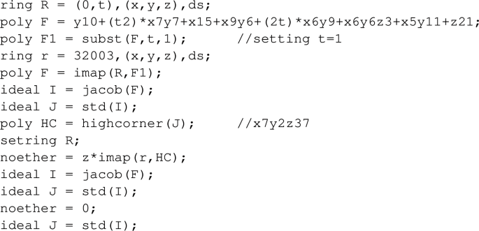
Comment on the Singular code:

• ring R = 0,(x,y,z),ds;: the ring ${\mathbb {Q}}[x,y,z]_{\langle x,y,z\rangle }$ with local degree reverse lexicographical ordering ds,

• ideal I = jacob(F),F;: the ideal generated by F and the partials of F,

• ideal J = std(I);: a standard basis in ${\mathbb {F}}_p[x,y,z]_{\langle x,y,z\rangle }$, $p=320039$,

• poly HC = highcorner(J);: the highest corner of J, $x^{24}z^7$in this case,

• noether = z*imap(r,HC);: the Singular command for truncating terms bigger (w.r.t. ds) than $z*HC$.

• ideal J = std(I);: a standard basis in ${\mathbb {Q}}[x,y,z]_{\langle x,y,z\rangle }$ using HC for truncation,

• noether = 0;: disables truncation during standard basis computation,

• ideal J = std(I);: a standard basis in ${\mathbb {Q}}[x,y,z]_{\langle x,y,z\rangle }$ not using HC.

The first 4 examples are computed over ${\mathbb {Q}}$ and $\mathbb F_p$. The Singular code is the same for the first 3 examples, with monomial ordering ds and computations in ${\mathbb {F}}_{32003}[y,x,z]_{\langle x,y,z\rangle }$ resp. in ${\mathbb {Q}}[y,x,z]_{\langle x,y,z\rangle }$.

• 1. $F = x^3y^3+x^5y^2+2x^2y^5+x^2y^2z^3+xy^7+z^9+y^{13}+x^{25},$

  $I = \langle F, \frac{\partial F}{\partial x},\frac{\partial F}{\partial y},\frac{\partial F}{\partial z}\rangle$.

• 2. $F = xyz(x+y+z)^2 +(x+y+z)^3 +x^{15}+y^{15}+z^{15}$,

  $I = \langle \frac{\partial F}{\partial x},\frac{\partial F}{\partial y},\frac{\partial F}{\partial z}\rangle$.

• 3. $F= x^8y^6+x^{10}y^5+x^8y^7+2x^7y^8+x^7y^6z^2+x^{16}+x^6y^{10}+y^{18}+z^{20},$

  $I = \langle \frac{\partial F}{\partial x},\frac{\partial F}{\partial y},\frac{\partial F}{\partial z}\rangle$.

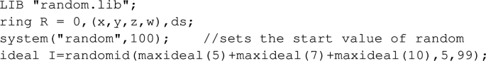
• 4. $I =$ ideal in the ring ${\mathbb {Z}}[x,y,z,w]_{\langle x,y,z,w\rangle }$ having 5 generators, which are random linear combinations of polynomials of degree 5, 7 and 10, with integer coefficients in the interval [-99,99]. The Singular code for creating this:

  

  In the following 4 examples the ring has a (single) parameter t and we want to compute the ideals in ${\mathbb {Q}}(t)[x,y,z]_{\langle x,y,z\rangle }$ resp. in ${\mathbb {Q}}(t)[x,y,z,w]_{\langle x,y,z,w\rangle }$. We set the parameter to $t=1$ to compute the highest corner in $\mathbb F_{32003} [y,x,z]_{\langle x,y,z\rangle }$ resp. in $\mathbb F_{32003}[x,y,z,w]_{\langle x,y,z,w\rangle }$.

  

• 5. $F = y^{10}+t^2x^7y^7+x^{15}+x^9y^6+2tx^6y^9+x^6y^6z^3+x^5y^{11}+z^{21},$

  $I = \langle \frac{\partial F}{\partial x},\frac{\partial F}{\partial y},\frac{\partial F}{\partial z}\rangle$.

• 6. $F = xyz(x+y+z)^2 +(x+y+z)^3 + t(x^{15}+y^{15}+z^{15})$,

  $I = \langle \frac{\partial F}{\partial x},\frac{\partial F}{\partial y},\frac{\partial F}{\partial z}\rangle$.

• 7. $F = x^8y^6+x^{10}y^5+x^8y^7+2x^7y^8+x^7y^6z^2+x^{16}+x^6y^{10}+ty^{18}+t^2z^{20}$,

  $I = \langle \frac{\partial F}{\partial x},\frac{\partial F}{\partial y},\frac{\partial F}{\partial z}\rangle$.

• 8. $I =$ ideal in the ring ${\mathbb {Z}}(t)[x,y,z,w]_{\langle x,y,z,w\rangle }$ having 5 generators, which are random linear combinations of polynomials of degree 5, 7 and 9, with integer coefficients in the interval [-99,99]. The Singular code for creating this:

  

Fig. 2

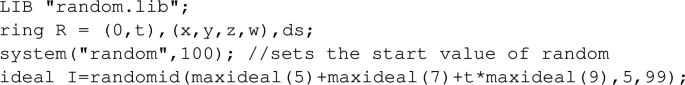
Table of timings

Timings

The examples were computed on a Linux machine with i7-6700 CPU @ 3.40 GHz. The times in the columns “Algorithm 5.1” (referring to our algorithm LocStdHC) and “std without HC” (referring to the usual standard basis algorithm), and “modStd” (referring to the modular algorithm described in Remark 5.5 (1)) are in seconds, $>2h$ means that the computation did not finish after 2 hours. RAM is the maximum memory requirement (for the usual algorithm) in MB. modStd is the modular standard basis algorithm in Singular, it is not implemented for rings with parameters.

References

Abbott, J., Kreuzer, M., Robbiano, L.: Computing Zero-dimensional Schemes. J. Symb. Comput. 39(1), 31–49 (2005)
Arnold, E.A.: Modular algorithms for computing Gröbner bases. J. Symb. Comput. 35(4), 403–419 (2003)
Decker, W., Greuel, G.-M., Pfister, G., Schönemann, H.: Singular 4-2-1 – A computer algebra system for polynomial computations (2021). http://www.singular.uni-kl.de
Greuel, G.-M., Pfister, G.: A Singular Introduction to Commutative Algebra. With contributions by O. Bachmann, C. Lossen and H. Schönemann. 2nd Edition, Springer, Berlin (2008)
Greuel, G.-M., Pfister, G.: Semicontinuity of Singularity Invariants in Families of Formal Power Series, arXiv:1912.05263v3 (2020). To appear in the Proceedings of the Némethi60 Conference
Matsumura, H.: Commutative Ring Theory. Cambridge University Press, Cambridge (1986)
Pfister, G.: On modular computation of standard basis. An. Stiint. Univ. Ovidius Constanţa, Ser. Mat. 15, No. 1, 129-138 (2007)
Acknowledgements
We like to thank the anonymous referees for useful comments and questions, which improved the presentation of the paper.
Funding
Open Access funding enabled and organized by Projekt DEAL.
Author information
Authors and Affiliations
Corresponding author
Additional information
Dedicated to the memory of Vladimir Gerdt.
Publisher's Note
Springer Nature remains neutral with regard to jurisdictional claims in published maps and institutional affiliations.
Missing Open Access funding information has been added in the Funding Note.
Rights and permissions
Open Access This article is licensed under a Creative Commons Attribution 4.0 International License, which permits use, sharing, adaptation, distribution and reproduction in any medium or format, as long as you give appropriate credit to the original author(s) and the source, provide a link to the Creative Commons licence, and indicate if changes were made. The images or other third party material in this article are included in the article’s Creative Commons licence, unless indicated otherwise in a credit line to the material. If material is not included in the article’s Creative Commons licence and your intended use is not permitted by statutory regulation or exceeds the permitted use, you will need to obtain permission directly from the copyright holder. To view a copy of this licence, visit http://creativecommons.org/licenses/by/4.0/.
About this article
Cite this article
Greuel, GM., Pfister, G. & Schönemann, H. Using Semicontinuity for Standard Bases Computations. Math.Comput.Sci. 16, 21 (2022). https://doi.org/10.1007/s11786-022-00539-2
Published:
DOI: https://doi.org/10.1007/s11786-022-00539-2