
Abstract
Non-stationary flood frequency analysis (FFA) is applied to statistical analysis of seasonal flow maxima from Polish and Norwegian catchments. Three non-stationary estimation methods, namely, maximum likelihood (ML), two stage (WLS/TS) and GAMLSS (generalized additive model for location, scale and shape parameters), are compared in the context of capturing the effect of non-stationarity on the estimation of time-dependent moments and design quantiles. The use of a multimodel approach is recommended, to reduce the errors due to the model misspecification in the magnitude of quantiles. The results of calculations based on observed seasonal daily flow maxima and computer simulation experiments showed that GAMLSS gave the best results with respect to the relative bias and root mean square error in the estimates of trend in the standard deviation and the constant shape parameter, while WLS/TS provided better accuracy in the estimates of trend in the mean value. Within three compared methods the WLS/TS method is recommended to deal with non-stationarity in short time series. Some practical aspects of the GAMLSS package application are also presented. The detailed discussion of general issues related to consequences of climate change in the FFA is presented in the second part of the article entitled “Around and about an application of the GAMLSS package in non-stationary flood frequency analysis”.
Introduction
The flood risk and design characteristics in the classical stationary approach are estimated using an upper quantile of annual maxima flow distribution with rank depending on the importance of protected areas or the class of high water prone structures. Typically the 99%-quantile (design quantile) of the annual maximum flow distribution is used which, under the stationary condition, corresponds to the return period of 100 years, i.e., so called 100-year water.
The changes in the land cover, water management activities in the catchment and a climate change in particular have made the hypothesis of the stationarity of flow extremes widely questionable which has led to the development of methods for non-stationary flood frequency analysis. It is commonly recognized that when researching the future there is no one efficient and totally certain method for making projections of statistical properties of floods under future climate conditions. The trend detection and analysis of observed data can only give us an idea of the future flood regime provided the present trend continues. This kind of future regime projections can be helpful in informed decision-making procedures; however, the way to introduce them into the design practice is long and bumpy. Note that even in stationary conditions changes in the design values due to the prolonged observation period are rarely taken into account in the risk assessment of breakdowns and failures of hydro-technical structures (Opyrchal 2005).
The estimation of trend in the upper quantiles of annual maximum flow depends on the choice of distribution and the method used for its assessment. Generally, even in the stationary conditions the flood frequency analysis is not based on the adequate probability model and in practice the distribution of annual or seasonal maxima is still unknown and lacks physical understanding. In hydrological practice and in many research studies a prior distribution is subjectively assumed (e.g., Kwon et al. 2008; Lima and Lall 2010), while the uncertainty related to that choice is often ignored. Hosking (1990); Mitosek et al. (2006); Strupczewski et al. (2006) and many others, tried to solve that problem by identifying the best (but not the true one) distribution from the available sample data and assessing the probability of the correct selection in specified cases. The problem of the best distribution choice becomes more complicated under the assumption of non-stationarity of the underlying process (there is no general theory for the distribution of extremes of nonstationary data). Moreover, some estimation methods [e.g., L-moments, or probability weighted moments (PWM)] are not suitable in that case.
In this study three approaches are compared: maximum likelihood method, two-stage method based on weighted least squares of simultaneous assessment of trends in the mean value and the standard deviation and the GAMLSS (generalized additive model for location, scale and shape parameters) approach. The comparison concerns only the point estimates of the 99%-quantile in order to show the differences resulting from the different approaches. The confidence intervals of the assessed values, although meaningful, are not included in the study.
The seasonal (winter and summer) maxima are more susceptible to climate variability and change due to possible changes in key climate drivers which are different in both seasons. There is a plethora of literature dealing with non-stationarity of flow extremes and their causes showing trends in climate indices, land use and the magnitudes of extreme flows themselves. We refer to them in our second paper in this issue entitled “Around and about an application of the GAMLSS package in non-stationary flood frequency analysis”. Here we propose a methodology to take account of non-stationary flood flows and we limit ourselves to three methods and their comparison, although others are possible, e.g., quantile regression methods (Koenker 2005) or Bayesian hierarchical estimation (Cheng et al. 2014; Yan and Moradkhani 2015, 2016).
A direct analysis of annual maxima series can mask important changes in seasonal dynamics, so it is important to use, if necessary and possible, seasonal stream-flow data in trend analysis, and not annual extremes which can sometimes fail to reveal the full temporal complexity of flow trends (Wilson et al. 2010). Moreover, seasonal series are expected to be more homogeneous than annual series in respect of both the distribution and trend. In his study the seasonal approach (SM) was used, assuming independence of winter and summer maxima.
Usually the estimation of time-dependent design quantiles is conditioned on a single model chosen from the set of candidate extreme value distributions. Here the multimodel approach was applied to reduce the model selection error which is an important source of uncertainty in the design quantiles especially when the observation series are short.
The time dependent 99%-quantiles resulting from three compared methods and the multimodel approach are presented for eight Polish and two Norwegian catchments chosen from the set of benchmark catchments of the Climate Change Impact on Hydrological Extremes (CHIHE) project (Romanowicz et al. 2016). These benchmark catchments are characterized by natural or quasi-natural hydrological regimes i.e., the flow generating processes are not altered significantly by human pressures and furthermore they represent the variability in climatic conditions across the two countries.
Those three methods were also compared with regard to their efficiency in detecting the known trends in flow maxima series and the 99%-quantile in the case of the true and false distribution assumptions. The comparison made by Monte Carlo experiments allows us to infer how the methods deal with model misspecification.
We begin with the descriptions of the seasonal approach, assumed trend models, three compared methods and multimodel aggregation (“Methodology”). “Case study: Polish and Norwegian catchments” provides the results of the comparison for Polish and Norwegian flood regimes. “Simulation study” deals with the evaluation of the performance and differences between the three non-stationary FFA approaches in quantifying trends in moments and design quantiles by the means of Monte Carlo simulations under the true and false distribution hypothesis. Final conclusions are drawn in “Conclusions”.
Methodology
Seasonal approach
The classical stationary model of annual maxima distribution in the seasonal approach is defined as the product of seasonal distributions under the assumption of independence between seasonal peak flow series (e.g., Guidelines for flood frequency analysis… 2005; Strupczewski et al. 2009, 2012; Vormoor et al. 2015, 2016; Debele et al. 2017). Thus, the cumulative distribution of annual maxima Y; Y = max(W,S) is given by:
where F w (y) and F s (y) are cumulative distributions of winter (W) and summer (S) maximum peak flows with parameter vectors θ W and θ S , respectively.
In the non-stationary case we assume that the distribution type remains the same and non-stationarity is manifested in the distribution parameters which are changing over time. This time dependence can be incorporated by time-varying covariates or simply by direct time dependence i.e., the parameters are deterministic functions of time. This second option has been applied in this study. Hence, under non-stationary conditions Eq. 1 can be written as:
The cumulative distribution functions of annual maxima defined by Eqs. 1 and 2 mostly have no explicit form for the quantile function so the quantiles ought to be found numerically.
Four 3-parameter (location μ, scale σ and shape k) distributions commonly applied in FFA were chosen for non-stationary analysis as the candidates for seasonal maxima models. Their probability density functions with corresponding first and second moments are given in Table 1. These distributions were used in the maximum likelihood and two-stage approaches. The distributions applied in GAMLSS are listed in the section describing the method.
Generally, there are two ways to incorporate time dependency into a distribution function parameters. It can be done by assuming trends in explicit distribution parameters or in distribution moments, more precisely in the mean and the standard deviation. The second method is recommended (Strupczewski and Kaczmarek 2001; Kochanek et al. 2013; Strupczewski et al. 2016). It enables mutual comparisons of the results obtained by different models and the classical climatological approach based on analysis of the variation of the mean and the standard deviation of climatic data over time. The shape parameter is assumed to be constant in time due to the high uncertainty of its estimation, even in the stationary case.
Trend models
As a result of the principle of parsimony, the assumed form of trends in mean and standard deviation ought to be as simple as possible. In this study, we tested several trend forms with one or two parameters, such as linear, logarithmic and exponential. The analysis confirmed the usefulness of linear trends in the form given by Eq. 3.
where t is time (in years following the beginning of the flood records), a and b are the slope and the intercept of the trend line for the mean, c and d, respectively, for the trend in standard deviation.
For each considered distribution model four options of trend analysis were taken into account in fitting the observed seasonal maxima:
-
1.
Option 0: stationary mean and the standard deviation.
-
2.
Option I: the mean value of the distribution varies linearly with time while the standard deviation remains constant.
-
3.
Option II: the mean value remains unchanged while the standard deviation varies linearly with time;
-
4.
Option III: the linear trend is reflected in both the mean and standard deviation of the distribution function.
Maximum likelihood method
The maximum likelihood (ML) method is one of the best known and widely used for fitting assumed probability distribution to the data. It produces asymptotically efficient and unbiased estimates of parameters, provided the assumed distribution is true. The estimates of distribution parameters are obtained by maximizing the log-likelihood function which in the case of trends considered here can be expressed as:
where f represents the density function, \(\varvec{ \theta }\) is the vector of trend model parameters [a, b, c, d] (see Eq. 3) and k denotes the shape parameter. As has been proved in Strupczewski and Feluch (1998); Strupczewski et al. (2001b), ML provides efficient estimators of time-dependent moments only in the case of long time series and the functional forms of distribution and trend approximating well the true forms. However, neither the true form nor the true distribution of the trend model is known; therefore, the results of ML estimation can be very uncertain.
Estimation of parameters was done with the help of the R software packages available on https://www.r-project.org/: extRemes (Gilleland and Katz 2016), FAdist (Aucoin 2015), PearsonDS (Becker and Klößner 2013).
Two-stage method
The method used for the assessment of the seasonal time dependent upper quantile is an adaptation of the so called two-stage (TS) method presented by, e.g., Strupczewski et al. (2016). The TS method consists of two stages:
-
An aggregate estimation of time-dependent mean and standard deviation performed by the weighted least squares (WLS) method (Strupczewski and Kaczmarek 2001; Strupczewski et al. 2016; Kochanek et al. 2013), standardization of the time series using the time-dependent moments, then estimation of constant shape parameters of the candidate distributions by means of the method of moments or (originally) L-moments and the calculation of the standardized quantiles.
-
The re-imposition of the trend on the values of the quantiles.
In the regression analysis the weighted least square method makes good use of small data sets. The method works by incorporating nonnegative weights, associated with each data point, into the fitting criterion. If the mean value is non-stationary then the trend in variance (or standard deviation) cannot be assessed separately. When the variance is nonstationary and unknown the system of equations ought to be solved for the linear form of trends in the mean and the standard deviation:
where y t —elements of time series, m t , s t —mean value and standard deviation in time t, m t = at + b; s t = ct + b. The equations are solved in respect of unknown trend model parameters.
Having found the values of trend parameters and corresponding values of mean and standard deviation the y t (=1, 2,…, T) values are standardized according to:
where z t are supposed to be realizations of stationary random variable Z with zero mean value and standard deviation equal to 1. The method of moments was used to estimate constant shape parameter of distribution of Z which is the same as the shape parameter of Y.
The re-imposition of the trend on quantiles estimated from standardized series is made by equation:
In the seasonal approach the TS method was applied to winter and summer seasons. Four candidate distributions listed in Table 1 for each seasonal maxima series were estimated. If the estimated shape parameter in GEV distribution was negative (i.e., the domain was upper bounded) then Gumbel distribution was chosen. Having estimated the parameters for each candidate distribution for standardized series z t , the stationary 99%-quantile was found. The trend re-imposition by Eq. 7 gives the non-stationary seasonal 99%-quantile for each candidate distribution.
In the comparisons presented below, we used two acronyms associated with the two-stage method. When we discuss the trend estimation, we use the WLS acronym, and when research involves the quantile comparison, WLS/TS or just TS is used.
GAMLSS approach
GAMLSS models were proposed by Rigby and Stasinopoulos (2005). They are semi-parametric, regression-type models; thus they require parametric and semi-parametric distributions. It is also a very general class of models for a univariate response variable. The models provide a common coherent framework for regression-type models, uniting models that are often considered as different in the statistical literature. In this study we used only a small part of the GAMLSS possibilities and facilities provided by the GAMLSS package implemented on R-project platform.
In the GAMLSS framework it is assumed that independent observations y i , for i = 1,…n, have a probability distribution function of \(f_{Y} \left( {y_{i} |\varvec{\theta}^{i} } \right)\) with \(\varvec{\theta}^{i} = \left( {\theta_{1}^{i} , \ldots ,\theta_{p}^{i} } \right)\) as a vector of p (p ≤ 4) parameters accounting for location, scale and shape of the distribution of random variable Y. In GAMLSS the distribution parameters are related to covariates by monotonic link functions g k (.). GAMLSS involves several models; in particular we use the fully parametric formulation (Eq. 8).
where \(\varvec{\theta}_{k}\) are vectors of length n, X k is a matrix of explanatory variables (i.e., covariates) of order n × m, \(\beta_{k}\) is a parameter vector of length m.
Three-parameter distributions with the lower bounds given in Table 1 are conventionally used in the FFA. However, only one distribution from the list can be found within the wide range (Rigby et al. 2014) of the GAMLSS distributions family—Weibull distribution (as in Table 1) in the reparameterized form of RGE (reverse-generalized-extreme) distribution (Table 2). Generally, the continuous distributions implemented in the GAMLSS package have a range of the response variable Y either (−∞, +∞) or (0, ∞) or (0, 1). In this study, we considered Weibull and three other GAMLSS distributions with zero lower bound and unbounded from the top, which we believe are close to, and suitable for, FFA distributions (Table 2). Among the GAMLSS pdfs presented in the Table 2, GG (generalized gamma) has been applied in hydrology by (López and Francés 2013; Zhang et al. 2015b).
Numerical optimisation methods (and corresponding software in R) for pdfs given in Table 2 require variable input information. Some of the methods require only the criterion function to be minimized, the other require the first derivative, the expected values of the second derivatives and the cross derivatives to be supplied as well. Some methods are more efficient than others but that depends on the criterion function being optimized. Some methods work when the others fail. Among the optimisation functions built in the R we used Optim, described as the general-purpose optimisation method based on the NelderMead (“Nelder-Meald”), quasi-Newton and conjugate gradient algorithms (i.e., “BFGS” “L-BFGS-B”). The Optim software includes the options for box-constrained optimisation and simulated annealing (”SANN”) and root-finding algorithm combining the bisection method, the secant method and inverse quadratic interpolation (“Brent”).
However, in many cases the optimization methods fail when maximizing the likelihood function using the Optim technique, especially when using covariates. To avoid this situation we used tools for general maximum likelihood estimation from the package bbmle (Bolker and R Development Core Team (2016), R Core Team (2017). The maximum likelihood estimation function and class in bbmle are both called mle2. It includes all the above mentioned numerical optimisation techniques as the options. In the mle2 package the optimisation methods is to be specified using the method argument (method=Optim” or others). We have found that the parameter estimates resulting from the mle2 function from package bbmle are much better and slightly more robust for finding the likelihood maximum than the standard R optimisation techniques.
Multimodel approach to seasonal maxima distributions
The problem of flood frequency modelling refers to the choice of the probability distribution describing the seasonal peak flows in line with the parameter estimation method and, therefore, quantiles of this distribution. In reality we do not know the true distribution function of flow maxima, thus the important source of uncertainty lies in the choice of seasonal maxima models, in particular of the dominant season. The use of multimodel approach is recommended, to reduce errors due to model misspecification in magnitude of quantiles. Conditioning on a single chosen model was criticized by (Draper 1995; Madigan and Raftery 1994), since it ignores model selection uncertainty and therefore leads to an underestimation of the uncertainty of quantities. Basic issues related to combining discriminatory and regression models are given by Burnham and (Anderson 2002; Gatnar 2008, and for FFA models by Bogdanowicz 2010; Markiewicz et al. 2015). Yan and Moradkhani (2015, 2016) proposed a multimodel ensemble approach by using the model averaging to predict the extreme flood in at site and regional context.
The multimodel approach can be regarded as a Bayesian inference procedure concerning e.g., design quantiles. Then, the quantile of interest, \(\bar{y}\left( F \right)\) in the stationary and \(\bar{y}\left( {F,t} \right)\) in the non-stationary case, can be treated as an average of the quantiles under each of the models considered, weighted by the corresponding posterior model probability expressed in terms of AIC or likelihood of candidate models (see Eqs. 10 and 12). In the non-stationary case, for each season and fixed time t, the multimodel approach was applied to find aggregated quantiles \(\bar{y}\left( {F,t} \right)\) resulting from considered candidate pdfs (Tables 1, 2) in the form of the weighted average:
where \(\hat{y}_{i} \left( {F,t} \right)\) is the estimate of F-quantile for time t of the i-th candidate model and the weights w i are defined by:
where m is the number of considered candidate pdfs; with δ i given by:
and AIC i represents the Akaike criterion values for maximized likelihood function of the i-th candidate distribution. When all models have the same number of parameters the weights can be calculated directly on the basis of the likelihood function values of each model:
L i being the maximized likelihood for the i-th model. The annual 99%-quantile in the multimodel approach in the non-stationary case should be found numerically by solving Eq. 13 with respect to p, for each t.
where \(F_{{W_{i} }}^{ - 1}\) and \(F_{{S_{j} }}^{ - 1}\) are the inverse cumulative distribution functions (quantile functions) of the i-th model for winter and j-th model for the summer season, respectively, the weights \(w_{i} {\text{and }}v_{j}\) are calculated using Eqs. 10 or 12 and they are constant in time. Finally, the annual 99%-quantile of the multimodel approach for each t is fund by substituting the resulting p into the aggregate time dependent quantile function of the winter or 0.99/p for the summer season (Eq. 9).
Trend model performance criteria
The deviance statistics was used (e.g., Coles 2001) to compare the performance of the different probability distribution models in fitting the observed seasonal maxima series under the different options of trends described above. With nested models \({\mathcal{M}}_{0 } \subset {\mathcal{M}}_{1}\), the deviance statistic is defined as:
where \(\ell_{1} \left( {{\mathcal{M}}_{1} } \right)\) and \(\ell_{0} \left( {{\mathcal{M}}_{0} } \right)\) are the maximized log-likelihood under models \({\mathcal{M}}_{1}\) and \({\mathcal{M}}_{0 }\), respectively. Assuming that the model \({\mathcal{M}}_{1}\) (larger) has k 1 parameters, so k 1 degrees of freedom, while the model \({\mathcal{M}}_{0 }\)(smaller) has k 0 parameters, the asymptotic distribution of \({\mathbf{\mathcal{D}}}\) is given by the \(\chi_{k}^{ 2}\) distribution with k = k 1 − k 0 degrees of freedom. The calculated value of \({\mathbf{\mathcal{D}}}\) can be compared to critical values from \(\chi_{k}^{ 2}\) for an assumed significance level, and large values of \({\mathbf{\mathcal{D}}}\) suggest that the larger model \({\mathcal{M}}_{1}\) explains substantially more of the variation in the data than the smaller \({\mathcal{M}}_{0}\). The maximized log-likelihood in the case of the TS method was assumed as the simple likelihood of the TS solution for the values greater than the median. The best-fitted trend model for each distribution type and estimation method was chosen according to the value of the deviance statistics.
Case study: Polish and Norwegian catchments
The catchments from the CHIHE project benchmark catchments was selected according to the criteria of the equilibrium in size of rain and thaw originated floods, when the seasonal approach is justified, i.e., there is no one dominating flood season. The location of selected catchments is shown in Fig. 1.

The location of the eight study catchments in Poland (a) and five study catchments in Norway (b). The Norwegian stations where the SM approach is justified and used in the case study are marked with red rectangles
The data series of the Polish catchments cover a period of 60 years (1951–2010) (see Table 3). Two selected Norwegian catchments Fustvatn and Krinsvatn have longer data series, respectively: 104 and 97 years. The daily data for Polish catchments were provided by the Institute of Meteorology and Water Management (IMGW) and for Norwegian catchments by the Norwegian Water Resources and Energy Directorate (NVE). Eight Polish catchments are mesoscale catchments (Fig. 1a) and vary in size from 275.5 km2 (Flinta) to 1083.7 km2 (Nysa Klodzka). Basic catchment characteristics including catchment area and some topographical information are given in Table 3. According to the principles of hydrological data processing introduced by the Polish Hydrological Service a water year runs from November 1 to October 31 and is divided into two seasons with fixed dates of the beginning and end; winter season from November to April with snowmelt floods and summer season from May to October with rainfall floods. The hydrological year in Norway and its division in seasons is discussed and defined by e.g., Vormoor et al. (2015) i.e., the summer season from March to August associated with snowmelt floods, and the winter season, from September to February associated with rainfall floods.
However, it should be emphasized that all the analyses given below are made on the basis of mean daily flow data according to CHIHE assumptions and requirements and their results in the form of upper quantiles cannot be treated as an evaluation of engineering design values.
Identification of the best distribution and trend models
The results of assessing trend in the mean and the standard deviation for all assumed distributions are presented in Table 4 (best fit model according to the AIC criterion). None of the considered options of time trend models identifies GAMLSS distributions family as the best one. The conformity of the best distribution type selection in winter season is almost perfect. Moreover, the ML and TS methods found the same best model with the same trend option for five catchments (see bold italic printed in Table 4). Stationary option (Option 0) has been identified as the best model three times by ML and four times by TS method. Whereas, for summer season the results are more diverse. The chosen best distribution types agree only in one case, the stationarity was detected as the best option in one catchment by ML and in five catchments by the TS method.
We consider option III for further analysis due to weak trends in the first two moments and the fact that quantiles are highly sensitive to the standard deviation values, so also to a trend in the standard deviation.
In this study we have found that the differences between the values of AIC for different fitted models and trend options are relatively small but they translate into considerable differences in time dependent moments and in the magnitude of upper quantiles. Moreover, the trend fitted by ML/GAMLSS methods under various distributional assumptions may even differ in sign. These results confirm former findings shown by (Strupczewski and Kaczmarek 2001; Strupczewski et al. 2001a, b). It is interesting to compare the values of time-dependent moments found under several distributional assumptions. The result of application of ML, WLS and GAMLSS approaches to estimate time-dependent mean and standard deviation for all candidate models are given in Table 5.
The results presented in Table 5 confirm the thesis that the ML and GAMLSS estimates of time-dependent moments are strongly distribution dependent, i.e., for the same time series but with different pdfs the detected trends can differ in their values and even in direction. It is obvious that the influence of distributional assumption on the values of ML and GAMLSS estimators of trend parameters is considerable, especially when the trends are weak. For instance, Weibull, Pearson type 3, RGE, LNO and Pearson type 3-GAMLSS give negative trends in the two first moments (see the bold printed figures in Table 5) while for the other models this trend is assessed as positive. The opposite trends in both seasons are related with different responses of the main seasonal flood generating processes to climate forcing mechanisms, but, obviously, one cannot assume that the computed trend will continue in the future.
The performance of the candidate non-stationary eight distribution models along with Option III was evaluated for 10 catchments. The significance of the detected trends was assessed by the deviance statistic (\({\mathbf{\mathcal{D}}}\), Eq. 14) to deal with the question of whether the non-stationary models provide an improvement in relation to the stationary counterparts. A non-stationary model with a greater number of parameters is also more flexible to reproduce the temporal variation of the data than a stationary one. The significance of the improvement was tested at the 0.05 significance level. The improvement was significant in PL4, PL5, PL6, PL7 and NOR1 in both seasonal distributions (except the TS estimates for winter). One can conclude (Table 4) that the majority of seasonal maxima flow series are identified as significantly non-stationary. Besides, in the case of ML and GAMLSS estimators the result of non-stationarity is hidden by the assumption of an underlying distribution.
Flood magnitude with a 0.01 exceedance probability was estimated. In this study, the time-dependent quantiles were presented and analyzed only for the catchments where:
-
1.
The seasonal trends in quantiles are opposite in terms of their direction, i.e., the upward-trend for the summer season and the downward for winter (PL3, Fig. 2a).
Fig. 2 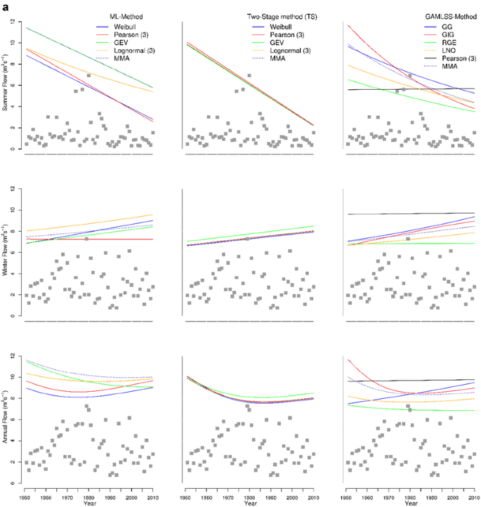
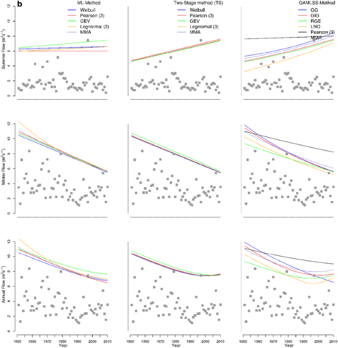
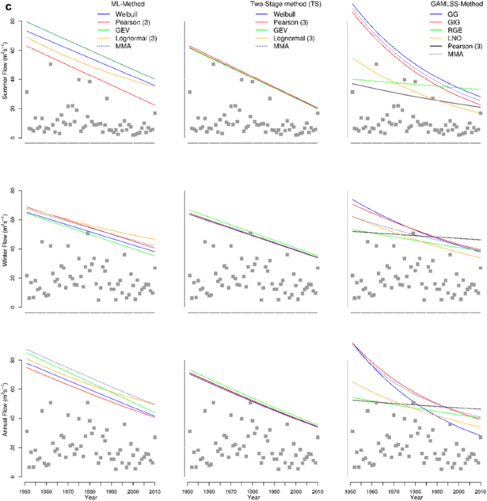
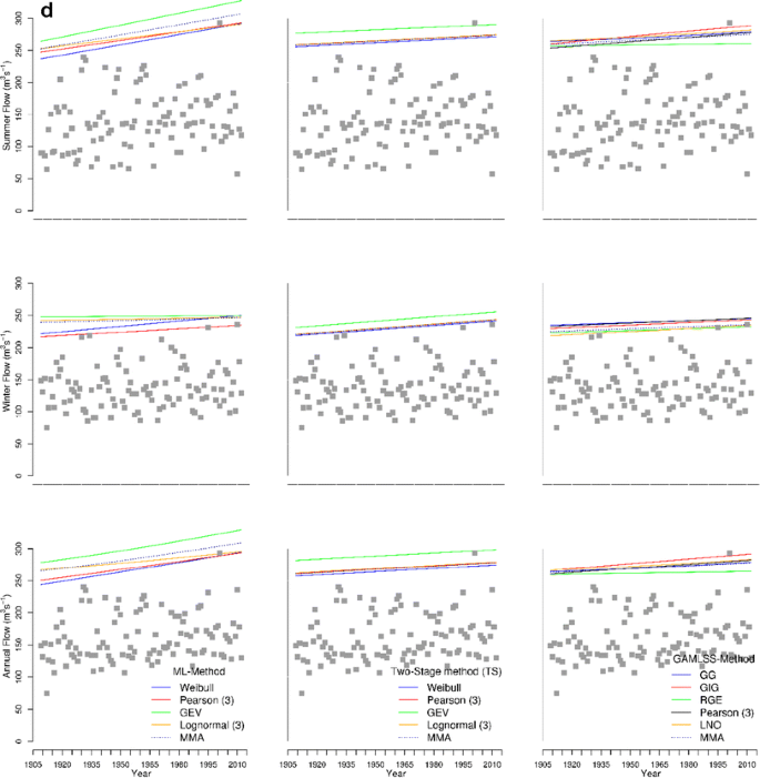
a PL3 seasonal and annual time dependent 99% quantiles (different trends). b PL4 seasonal and annual time dependent 99% quantiles (different seasonal trends). c PL5 seasonal and annual time dependent 99% quantiles (both seasonal trends decreasing). d NOR1 seasonal and annual time dependent 99% quantiles (equal share of winter and summer maxima in upper limb of AM)
-
2.
The seasonal trends in quantiles are opposite in terms of their direction, i.e., the downward-trend for the summer season and the upward for winter (PL4, Fig. 2b).
-
3.
The seasonal trends in quantiles have the same direction (here descending trends) (PL5, Fig. 2c).
-
4.
The seasonal maxima have a similar share in the upper limb of the annual maxima distribution (NOR1, Fig. 2d).


From the results presented in Fig. 2a–d, one can easily see that the variability of the time-dependent design quantile estimates with regard to model choice is much lower for TS than ML and GAMLSS approaches, i.e., the TS approach is the most distribution-free method among three methods considered here. This is the advantage of using the TS method in non-stationary FFA when the true pdf is unknown and the time-series are of limited length.
The SM approach results in a more realistic form of the trend in annual maxima compared to the direct analysis of annual maxima when a linear trend model is assumed. This is due to taking into account the different effects of climate forcing on the main seasonal flood generation processes. For instance, the curved shape of the annual 99%-quantile for the TS approach depicted in Fig. 2a, b is obtained due to a SM trend analysis and it will never be achieved by direct analysis of annual maxima series with a linear trend in moments. Furthermore, the gain in the identification of a trend in annual maxima will increase if both seasonal maxima have a similar share in the annual maxima series (Fig. 2d). It can also be found that the variability in estimates of 99% time-dependent quantiles is larger in the summer than in the winter season. Contrary to popular opinion, the trends in the winter season are not always stronger than in the summer.
Multimodel approach: time-dependent design quantiles
The application of a multimodel approach (MMA) is the way to overcome uncertainty of time-dependent design quantile estimates due to hypothetical distribution assumption and to alleviate the effect of differences in trends obtained by using different models. Besides, MMA is also useful in reducing underestimation of the uncertainty of quantiles of interest. The estimates of the time-dependent multimodel 99%-quantile, \(\bar{y}\left( {0.99;t} \right)\), of seasonal and annual maxima obtained by the three estimation methods (Eq. 12) at \(t = 1, N/2\) and N are presented in Table 6.
As it can be seen in Table 6 and Fig. 2a–d, the multimodel time-dependent design quantiles (dark blue dotted lines) obtained by solving Eq. 9 alleviate the variability of the time-dependent design quantile obtained from different models, and make them less distribution dependent. Obviously, the resulting multimodel 99% quantiles are close to the distribution with largest weight among the selected distribution in the case of the estimation of seasonal maxima. In the case of annual maxima based on the multimodel approach the estimates of annual 99%-quantile are closer to the distribution of the dominated season. In most of the considered catchments, including the results not presented here, the MMA quantiles are larger for the ML and GAMLSS methods than for the TS method.
Simulation study
The results of the quantile estimation in stationary and non-stationary FFA depend strongly on the estimation method. The Monte Carlo simulation study was carried out to compare the efficiency of ML, GAMLSS and TS methods in estimation of the true and false non-stationary distributions. In particular, we compared three non-stationary FFA methods with regard to the estimates of the parameters of trends in moments and the estimates of 99%-quantile for various sample sizes. The aim of comparison was to find the most robust method of non-stationary FFA in respect to trend detection and 99%-quantile accuracy for a given sample size. We considered the case of time dependent mean and standard deviation (Option III).
To make the simulations more realistic, the linear trend models for the mean value and the standard deviation for the true i.e., parent population were chosen such as they are actually observed in the data. That is why we have taken WLS estimation results for the Nysa Klodzka river as the true trends for simulations experiments. The comparison has been made for two pairs of hypothesis. The first pair concerns the situation when the assumed distribution is the same as the parent (H = T) and the second pair when the assumed distribution is not the same, i.e., false (H = F). As the distributions used in the GAMLSS approach (Table 2) do not coincide with FFA distributions (Table 1) used in the ML and TS methods (except Weibull i.e., RGE in GAMLSS and Pearson 3 distribution added to the GAMLSS family), the possibilities of H = T and H = F are limited. Here we show only the results of the simulation for the following configuration of the true–false hypothesis:
-
GEV = T with GEV = T, simply denoted as GEV = T
-
Lognormal (3) = F with GEV = T,
-
RGE = T, with RGE = T, simply denoted as RGE = T
-
RGE = F with Lognormal (3) = T,
The first two configurations enable us to compare only the ML method with the TS. The studies by Markiewicz et al. (2010); Strupczewski et al. (2016) involved with comparison of the accuracy of the ML and TS methods for various distributions and Monte Carlo simulated sample sizes. Here, we present only the results of the first two configurations mentioned above. The relative bias (RB) and relative root mean square error (RRMSE) of the estimates (parameters of trend in moments, constant skewness and a time dependent quantile \(\hat{y}_{F}\) for non-exceedance probability F = 0.99) were based on 10,000 simulations with a sample size of \(N = 50, 100 {\text{and }}200\) generated from the assumed parent distribution. Considered lengths of simulated time series correspond to the lengths we normally have in hydrology. The quantiles and their estimation errors were calculated for t = 1, N/2 and N, i.e., at the beginning, in the middle and at the end of observation period. In tables below (Tables 1,2) the best results are printed in bold.
The cases: GEV = T; Lognormal (3) = F with GEV = T; RGE = T
Results are presented for the parent time-dependent mean and standard deviation, \({\text{m}}\left( {\text{t}} \right) = 0. 8 8 \times {\text{t}} + 4 2. 8 1,{\text{ s}}\left( t \right) = 0. 3 9 \times {\text{t}} + 1 8. 7 7\) and skewness equal to 1.71. In Table 7, the |RRMSE| of the estimated trend parameters \(\hat{a},\hat{b},\hat{c},\hat{d}\) are presented (ML and WLS) and the RRMSE and RB of the quantile estimates \(\hat{y}_{F}\) (F = 0.99) in the ML, TS and GAMLSS are shown in Table 8.
The values of the relative bias of quantile estimators vary within a few percent and decrease with the length of time-series (see left columns of Tables 7, 8). Based on the simulation results of the skewness coefficient C s (not presented here) both RB and RRMSE decrease with increasing length of the time-series but vary largely. In Table 7, one can see the advantage of the estimates of all four parameters revealed by the WLS method; thus, applying WLS in non-stationary FFA rather than ML is recommended. Generally, as can be seen in Table 8, TS provides smaller \({\text{RRMSE}}\left( {\hat{y}_{F} } \right)\) and slightly higher \({\text{RB }}\left( {\hat{y}_{F} } \right)\) in the estimates of the 99% quantile. The simulations confirm that under the hypothesis specified above, TS is the best method for short hydrological time-series, i.e., N ≈ 50. The ML estimator produced lower RB but higher RRMSE values. Thus, if one compares only the obtained values of RRMSE in both methods, the TS method leads to better estimates than ML. For longer hydrological time-series the differences between RRMSE from ML and TS methods are smaller. Table 8 supports the conclusion made in the literature: high RRMSE values are due to the large ML estimator variance, caused by a few outliers influencing the value of the skewness, i.e., the shape parameter k.
The cases: RGE = T; RGE = F with Lognormal (3) = T
The advantages and disadvantages of GAMLSS methods when a true distribution function is known and the false is assumed have not been studied so far. The reverse-generalized-extreme (RGE) (Table 2) which is a reparameterization of the three-parameter Weibull distribution, often used in FFA, served here as the parent distribution (H = T). A Monte Carlo simulation experiment is designed in the same way as mentioned above. The comparison was made for time-dependent mean and standard deviation;\(m\left( t \right) = 0.94 \times t + 89.19, \, \sigma \left( t \right) = 0.92 \times t + 60.11\) and constant skewness is equal to 1.14. Table 9 presents the |RRMSE| of the trend parameters for moments from the GAMLSS and WLS methods.
The results presented in Table 9 show that the relative accuracy of the estimation of all four parameters presents a similar pattern for both methods. The RRMSE increases with the decreasing length of the time-series. In particular, results in Table 9, which are printed in bold, prove clearly the advantage of the accuracy of estimates of the trend in standard deviation obtained from the GAMLSS method, while WLS provides better accuracy in the estimates of the trend in the mean value. In both methods this advantage decrease gradually with increasing length of the time-series.
Based on the result of RB and RRMSE of the skewness (not presented here) the GAMLSS estimator of \(\hat{C}_{s}\) maintains the advantage over TS for all examined lengths of time-series. However, the RB \(\left( {\hat{C}_{s} } \right)\) and RRMSE \(\left( {\hat{C}_{s} } \right)\) from both methods showed regular variation and they decrease with increasing time-series length. Table 8 reports the RB and the RRMSE values for the 99%-quantile estimates by GAMLSS and TS methods. The result demonstrates that the GAMLSS method performed better than the TS method especially for longer time-series (Table 8). This is not surprising; rather it confirms our result obtained for parameter estimates, i.e., upper quantiles are highly dependent on errors in standard deviation and shape (k), so, as noted above, GAMLSS produces smaller |RB| and RRRMSE in estimates of the standard deviation and the shape parameter k.
When a false model is assumed, the errors of \(\hat{C}_{s}\) by the two approaches increase. However, the increase is the largest for the ML method. Table 10 (in left column) presents the RB and RRMSE of the 99%-quantile estimator value. The results are consistent with the results obtained under the true hypothesis. When we assumed H = T = RGE, the ML gives a smaller bias and relatively larger RRMSE than the TS method. One can also get the opposite results by replacing H = F; the ML method gives smaller RRMSE, and a relatively larger bias (bold printed values in Tables 8, 10).
When RGE is assumed as a false distribution, the efficiency of GAMLSS algorithm can be assessed. The Monte Carlo Simulation experiment was implemented in a similar way as in the case of a true hypothetical distribution. The Lognormal (3) was taken as true distribution (H = T) and time-dependent moments, shape parameter k and 99%-quantile were estimated. Table 9 (right column) provide |RRMSE| of the estimated trend parameters in moments and Table 10 (right column) RRMSE and RB of the 99%-quantile estimates. As it could be expected the errors obtained for the estimated trend parameters for moments, skewness coefficient and 99%-quantile are higher than those obtained for the true case (H = T=RGE). In general, it can be seen from Table 10 that the GAMLSS method was again better than the TS method in terms of the RB and RRMSE obtained for 99%-quantile (bold printed values in Table 10 similar as for the H = F case. Note that in all Monte Carlo simulation experiments, the result depends strongly on the chosen values of the trend parameters.
Table 7 (right column) reports the RRMSE of the trend parameters for the mean and standard deviation. Based on Table 10 (left column) the ML estimates of trend slopes \(\left( {{\hat{\text{a}}},{\hat{\text{c}}}} \right)\) differ significantly from true ones. Even the percentage difference of \({\hat{\text{a}}},{\hat{\text{c}}}\) obtained from H = T = RGE and H = F = RGE increase with the length of the hydrological time-series. Therefore, one can notice the difficulties associated with a short length of the hydrological time-series in discrimination of the true distribution from the false one. The RRMSE \(\left( {\hat{C}_{s} } \right)\) and \({\text{RB}}\left( {\hat{C}_{s} } \right)\) of the skewness coefficient estimator (not shown) in both methods does not exhibit regular variations. The ML produced higher RRMSE \(\left( {\hat{C}_{s} } \right)\) and \({\text{RB}}\left( {\hat{C}_{s} } \right)\) than the TS method.
Conclusions
Seasonal non-stationary FFA has been examined through a statistical analysis of seasonal flow maxima from Polish and Norwegian catchments. Throughout the study, three non-stationary methods; namely, maximum likelihood (ML), two stage (TS) and GAMLSS were applied and compared with the aim of capturing the effect of non-stationarity in the estimation of time-dependent moments and design quantile. Numerous hydrological studies successfully applied GAMLSS in non-stationary FFA (Machado et al. 2015; Villarini et al. 2009a, b, 2010a, b, 2012; Zhang 2015a), but most were addressing two parameter distributions, which are rarely used in hydrological practice. The standard pdfs commonly used in water resources engineering hydrological designs are three parameter distributions with a lower bound as location parameter, such as Weibull, Pearson 3, Lognormal 3 and GEV in which the lower bound (if it exists, i.e., k > 0) is equal to \(\mu - \sigma \,/\,k\); so their domain is not fixed in a non-stationary modelling. However, these standard pdfs, except Weibull, are not explicitly implemented in GAMLSS algorithms. The GAMLSS model has a major advantage over the ML and TS methods; for example, an easy addition of extra distributions and allowing different model diagnostics for each distribution parameter.
Among distributions commonly used in FFA, the Pearson type 3 distribution was successfully introduced into the GAMLSS algorithms. Three-parameter Weibull, in a re-parameterised form of RGE distribution in GAMLSS software was applied for the first time in non-stationary FFA. However, we failed to implement GEV and Lognormal type 3 into GAMLSS fitting algorithms. Due to the fact that upper quantiles are highly sensitive to changes in standard deviation and shape parameter, we assumed a constant shape and linear trend in the mean and standard deviation values. The results from the present study have confirmed that it is important to identify non-stationarity in the first two moments and to extend it in frequency analysis. The best pdf and time trend in the first two moments, from the considered models, were selected. The results of the analyzed dataset showed that the ML and GAMLSS estimates of time-dependent moments were strongly distribution dependent. Thus, the influence of the distribution choice on the values of the ML and GAMLSS estimators of trend are considerable. The overall assessment of the deviance statistics \({\mathbf{\mathcal{D}}}\) confirmed that the TS method provides more evidence for nonstationarity (43.75%) and it is followed by the GAMLSS (42.5%) method. A comparison of the estimated moments achieved by the WLS, ML and GAMLSS methods shows larger consistency for the winter season than for the summer.
The TS method showed smaller variability in the estimates of the 99%-quantile than the ML and GAMLSS methods; whereas, the estimated values are higher for ML and GAMLSS. Following the results from three non-stationary FFA approaches, a 30% decreasing and 70% increasing tendency of the design quantile are observed for winter and summer, mainly in mountainous Polish rivers. On the other hand, the estimates of 99%-quantiles based on annual maxima showed 50% increasing and 50% decreasing tendencies. The main sources of uncertainty in the accuracy of flood quantile estimates, regardless of sample size are: (1) the choice of seasonal maxima distribution and (2) estimation based on a single final model. This problem can be alleviated by using multimodel approach. The results from the present study have clearly pointed out that the application of a multimodel approach to 99%-quantile estimates alleviated the variability of the time-dependent 99% quantiles obtained from different models. Generally, the MMA approach was more successful when the considered models had similar weights. Generally, the non-stationarity analysis produced more accurate estimates of the moments and 99% quantiles. The question arises as to whether it is necessary to include non-stationarity, i.e., regardless of computational difficulties and weak non-stationarity, in practical applications.
An analysis based on the observed seasonal maxima has supported the use of the TS method rather than ML and GAMLSS in the non-stationary FFA when the true pdf of seasonal flow maxima is unknown. The computer simulations were performed by means of a Monte Carlo experiment to compare the efficiency of the three non-stationary FFA methods with time as a covariate. The comparison of the estimation methods ML and TS, with a simulation experiment shows that, under the true and false hypothesis, the WLS/TS method produces the best results with respect to RRMSE; whereas, in the case of the RB ML method it achieved smaller values than the TS method. Generally, the simulation experiment for the case of truly and falsely assumed pdfs (while comparing the ML and the TS methods) used to estimate moments showed that the TS method proved better than the ML method, particularly for shorter hydrological series.
The results of the experiment showed that for truly and falsely assumed pdf, GAMLSS produced the best results with respect to RB and RRMSE for estimates of trends in standard deviation and the skewness coefficient, while WLS/TS provided better accuracy in estimates of trends in the mean value. The higher probability (0.99) quantiles are more sensitive to the errors in standard deviation than in the mean and the shape parameter k; thus, the overall simulation experiment has demonstrated that the GAMLSS method performed better than the TS method, especially for longer sample sizes. Still the TS method proved to be the best estimator for small sample sizes and trends in the mean values. In conclusion, study we have critically evaluated three non-stationary FFA methods based on the observed data and computer simulation from the view of the time-dependent moment and design quantile. Also, we have proposed and demonstrated a method on how to deal with the uncertainties that arise from model misspecification. Further work will focus on the GAMLSS framework from the point of view of its practical application and improving the simulation speed of the algorithms.
References
Aucoin F (2015) FAdist: distributions that are sometimes used in hydrology. R package version 2.2. https://CRAN.R-project.org/package=FAdist
Becker M, Klößner S (2013) PearsonDS: Pearson distribution system. R package version 0.97. http://CRAN.R-project.org/package=PearsonDS
Bogdanowicz E. (2010) Multimodel approach to estimation of extreme value distribution quantiles. Podejście wielomodelowe w zagadnieniach estymacji kwantyli rozkładu wartości maksymalnej. In: Hydrologia w inżynierii i gospodarce wodnej. Tom 1, Ed. B. Więzik. Monografie Komitetu Inżynierii Środowiska, 68, (in Polish)
Bolker B, R Development Core Team (2016) bbmle: tools for general maximum likelihood estimation. R package version 1.0.18. https://CRAN.R-project.org/package=bbmle
Burnham KP, Anderson DR (2002) Model selection and multimodel inference. Springer, New York
Cheng L, AghaKouchak A, Gilleland E, Katz RW (2014) Non-stationary extreme value analysis in a changing climate. Clim Change 127:353–369. doi:10.1007/s10584-014-1254-5
Coles SG (2001) An introduction to statistical modeling of extreme values. Springer, London
Debele SE, Bogdanowicz E, Strupczewski WG (2017) The impact of seasonal flood peak dependence on annual maxima design quantiles. Hydrol Sci J. doi:10.1080/02626667.2017.1328558
Draper D (1995) Assessment and propagation of model uncertainty (with discussion). J R Statist Soc B 57:45–97. doi:10.1515/acgeo-2015-0070
Gatnar E (2008) Podejście wielomodelowe w zagadnieniach dyskryminacji i regresji (Multimodel approach to issues of discrimination and regression). PWN, Warszawa (in Polish)
Gilleland E, Katz RW (2016) extRemes 2.0: an extreme value analysis package in R. J Stat Softw 72(8):1–39. doi:10.18637/jss.v072.i08
Guidelines for flood frequency analysis long measurement series of river discharge (2005) WMO/HOMS Component I81.3.01. http://www.wmo.int/pages/prog/hwrp/homs/Components/English/i81301.htm. Accessed Apr 2017
Hosking JRM (1990) L-moments: analysis and estimation of distributions using linear combinations of order statistics. J Roy Stat Soc B 52:105–124
Kochanek K, Strupczewski WG, Bogdanowicz E, Feluch W, Markiewicz I (2013) Application of a hybrid approach in nonstationary flood frequency analysis—a Polish perspective. Nat Hazards Earth Syst Sci Discuss 1(5):6001–6024. doi:10.5194/nhessd-1-6001-2013
Koenker R (2005) Quantile Regression. Cambridge Books, Cambridge University Press, New York
Kwon H-H, Brown C, Lall U (2008) Climate informed flood frequency analysis and prediction in Montana using hierarchical Bayesian modeling. Geophys Res Lett. doi:10.1029/2007GL032220
Lima CHR, Lall U (2010) Spatial scaling in a changing climate: a hierarchical bayesian model for nonstationary multi-site annual maximum and monthly streamflow. J Hydrol 383:307–318. doi:10.1016/j.jhydrol.2009.12.045
López J, Francés F (2013) Non-stationary flood frequency analysis in continental Spa-nish rivers, using climate and reservoir indices as external covariates. Hydrol Earth Syst Sci 17:3189–3203. doi:10.5194/hess-17-3189-2013
Machado MJ, Botero BA, López J, Francés FA, Díez-Herrero BG (2015) Flood frequency analysis of historical flood data under stationary and non-stationary modelling. Hydrol Earth Syst Sci 19:2561–2576. doi:10.5194/hess-19-2561-2015
Madigan D, Raftery AE (1994) Model selection and accounting for model uncertainty in graphical models using Occam’s window. J Am Statist Assoc 89:1535–1546
Markiewicz I, Strupczewski WG, Kochanek K (2010) On accuracy of upper quantiles Estimation. Hydrol Earth Syst Sci 14:2167–2175. doi:10.5194/hess-14-2167-2010
Markiewicz I, Strupczewski WG, Bogdanowicz E, Kochanek K (2015) Generalized exponential distribution in flood frequency analysis for Polish. Rivers. doi:10.1371/journal.pone.0143965
Mitosek HT, Strupczewski WG, Singh VP (2006) Three procedures for selection of annual flood peak distribution. J Hydrol 323:57–73. doi:10.1016/j.hydrol.2005.08.016
Opyrchal L (2005) Metoda analizy i oceny ryzyka awarii opracowana dla polskich budowli hydrotechnicznych (Method of analysis and risk assessment of breakdown for Polish hydrotechnical structures), Materiały Badawcze, Instytut Meteorologii i Gospodarki Wodnej, Seria: Inżynieria Wodna, 0239-6254; 17 (in Polish)
R Core Team (2017) R: a language and environment for statistical computing. R Foundation or Statistical Computing, Vienna. ISBN 3-900051-07-0
Rigby RA, Stasinopoulos DM (2005) Generalized additive models for location, scale and shape. Appl Stat 54:507–554. doi:10.1111/j.1467-9876.2005.00510
Rigby RA, Stasinopoulos DM, Heller G, Voudouris V (2014) The distribution Toolbox of GAMLSS. (http://www.gamlss.org/wp-content/uploads/2014/10/distributions.pdf)
Romanowicz RJ, Bogdanowicz E, Debele SE, Doroszkiewicz J, Hisdal H, Lawrence D, Meresa HK, Napiórkowski JJ, Osuch M, Strupczewski WG, Wilson D, Wong WK (2016) Climate change impact on hydrological extremes: preliminary results from the polish-norwegian project. Acta Geoph 64(2):477–509. doi:10.1515/acgeo-2016-0009
Strupczewski WG, Feluch W (1998), Investigation of trend in annual peak flow series. Part I. Maximum likelihood estimation. In: Proceedings 2nd international conference on climate and water—A 1998 perspective, 17–20 August 1998, Espoo, Finland, vol 1. p 241–250
Strupczewski WG, Kaczmarek Z (2001) Non-stationary approach to at-site flood frequency modelling. Part II. Weighted least squares estimation. J Hydrol 248(1–4):143–151. doi:10.1016/S0022-1694(01)00398-5
Strupczewski WG, Singh VP, Mitosek HT (2001a) Non-stationary approach to at-site flood frequency modelling. Part III. Flood analysis of Polish rivers. J Hydrol 248(1–4):152–167. doi:10.1016/S0022-1694(01)00399-7
Strupczewski WG, Singh VP, Feluch W (2001b) Non-stationary approach to at-site flood frequency modelling. Part I. Maximum likelihood estimation. J Hydrol 248(1–4):123–142. doi:10.1016/S0022-1694(01)00397-3
Strupczewski WG, Mitosek HT, Kochanek K, Singh VP, Weglarczyk S (2006) Probability of correct selection from lognormal and convective diffusion models based on the likelihood ratio. Stoch Environ Res Risk Assess 20:152–163. doi:10.1007/s00477-005-0030-5
Strupczewski WG, Kochanek K, Feluch W, Bogdanowicz E, Singh VP (2009) On seasonal approach to nonstationary flood frequency analysis. Phys Chem Earth 34:612
Strupczewski WG, Kochanek K, Bogdanowicz E, Markiewicz I (2012) On seasonal approach to flood frequency modelling, Part I: flood frequency analysis of Polish rivers. Hydrol Process 26:705–716. doi:10.1002/hyp.8179
Strupczewski WG, Kochanek K, Bogdanowicz E, Markiewicz I, Feluch W (2016) Comparison of two nonstationary flood frequency analysis methods within the context of the variable regime in the representative polish rivers. Acta Geoph 64(1):206–236. doi:10.1515/acgeo-2015-0070
Villarini G, Serinaldi F, Smith JA, Krajewski WF (2009a) On the stationarity of annual flood peaks in the continental United States during the 20th century. Water Resour Res 45:1–17
Villarini G, Smith JA, Serinaldi F, Bales J, Bates PD, Krajewski WF (2009b) Flood frequency analysis for nonstationary annual peak records in an urban drainage basin. Adv Water Resour 32:1255–1266. doi:10.1029/2008WR007645
Villarini G, Smith JA, Napolitano F (2010a) Nonstationary modelling of a long record of rainfall and temperature over Rome. Adv Water Resour 33:1256–1267
Villarini G, Vecchi GA, Smith JA (2010b) Modeling the dependence of tropical storm counts in the North Atlantic basin on climate indices. Mon Weather Rev 138:2681–2705
Villarini G, Smith JA, Serinaldi F, Ntelekos AA, Schwarz U (2012) Analyses of extreme flooding in Austria over the period 1951–2006. Int J Climatol 32:1178–1192. doi:10.1002/joc.2331
Vormoor K, Lawrence D, Heistermann M, Bronstert A (2015) Climate change impacts on the seasonality and generation processes of floods—projections and uncertainties for catchments with mixed snowmelt/rainfall regimes. Hydrol Earth Syst Sci 19:913–931. doi:10.5194/hess-19-913
Vormoor K, Lawrence D, Schlichting L, Wilson D, Wong WK (2016) Evidence for changes in the magnitude and frequency of observed rainfall vs. snowmelt driven floods in Norway. J Hydrol 538:33–48
Wilson D, Hisdal H, Lawrence D (2010) Has streamflow changed in the Nordic countries? Recent trends and comparisons to hydrological projection. J Hydrol 394(3–4):334–346
Yan H, Moradkhani H (2015) A regional Bayesian hierarchical model for flood frequency analysis. Stoch Env Res Risk Assess 29(3):1019–1036. doi:10.1007/s00477-014-0975-3
Yan H, Moradkhani H (2016) Toward more robust extreme flood prediction by Bayesian hierarchical and multimodeling. Nat Hazards 81(1):203–225. doi:10.1007/s11069-015-2070-6
Zhang Q, Gu X, Singh VP et al (2015a) Evaluation of flood frequency under non-stationarity resulting from climate indices and reservoir indices in the East River basin, China. J Hydrol 527:565–575. doi:10.1016/j.jhydrol.2015.05.029
Zhang D, Yan D, Wang YC, Lu F, Liu S (2015b) GAMLSS-based nonstationary modeling of extreme precipitation in Beijing–Tianjin–Hebei region of China. Nat Hazards 77:1037–1053. doi:10.1007/s11069-015-1638-5
Acknowledgements
This research has been done in the framework of Polish-Norwegian Research Programme project CHIHE (PolNor/196243/80/2013), carried out by the Institute of Geophysics, Polish Academy of Sciences and partially supported within statutory activities No 3841/E-41/S/2017 of the Ministry of Science and Higher Education of Poland. We would like to gratefully acknowledge Robert A. Rigby and Dimitrios M. Stasinopoulos for their help in GAMLSS modelling framework.
Author information
Authors and Affiliations
Corresponding author
Rights and permissions
Open Access This article is distributed under the terms of the Creative Commons Attribution 4.0 International License (http://creativecommons.org/licenses/by/4.0/), which permits unrestricted use, distribution, and reproduction in any medium, provided you give appropriate credit to the original author(s) and the source, provide a link to the Creative Commons license, and indicate if changes were made.
About this article

Cite this article
Debele, S.E., Strupczewski, W.G. & Bogdanowicz, E. A comparison of three approaches to non-stationary flood frequency analysis. Acta Geophys. 65, 863–883 (2017). https://doi.org/10.1007/s11600-017-0071-4
Received:
Accepted:
Published:
Issue Date:
DOI: https://doi.org/10.1007/s11600-017-0071-4