
Abstract
In the last 30 years, there are many publications in the literature due to global warming and climate change impacts exhibiting non-stationary behaviors in hydro-meteorology time series records especially in the forms of increasing or decreasing trends. The conventional trend analyzes cover the entire recording time with a single straight-line trend and slope. These methods do not provide information about up and down partial moving trends evolution at shorter durations along the entire record length. This paper proposes a dynamic methodology for identifying such evolutionary finite duration moving trend method (MTM) identifications and interpretations. The purpose of choosing MTM was to investigate the dynamic partial trend evolution over the recording period so that dry (decreasing trend) and wet (increasing trend) segments could be objectively identified and these trends could assist in water resources management in the study area. The moving trend analysis is like the classical moving average methodology with one important digression that instead of arithmetic averages and their horizontal line representations, a series of finite duration successive increasing and decreasing trends are identified over a given hydro-meteorology time series record. In general, partial moving trends of 10-year, 20-year, 30-year and 40-year occur above or below the overall trend and thus provide practical insight into the dynamic trend pattern with important implications. The moving trend methodology is applied to annual records of Danube River discharges, New Jersey state wise temperatures and precipitation time series from the City of Istanbul.
1 Introduction
Global warming due to greenhouse gas (GHG) released into the troposphere causes climate change, which can reflect itself as partial and overall increasing or decreasing trends in any hydro-meteorological time series. It has already been proven by Milly et al. (2008) that all hydro-meteorological records fall into non-stationary realm with the inclusion of trends. Hydro-meteorological records have systematic components such as trends and variability (Burn and Hag Elnur 2002). There are basic methodological contributions that provide probabilistic or statistical trending tests (Mann 1945; Kendal 1970; Spearman 1904; Sen 1968; IPCC 2007; Şen 2012; Alashan 2018; Güçlü 2018; Ashraf et al. 2021). The applications of these methods have increased in an unprecedented way and therefore there are many studies in different disciplines that try to determine the overall (holistic) trend. Hamed (2008) has proposed different trend detection methodologies in hydro-meteorology records. A review of current trend methodologies is presented by Sonali and Kumar (2013) and applied these methodologies to temperature records. One of the major problems in the Mann and Kendall (MK) trend identification methodology is the assumption that time series must be serially independent, which cannot be met with hydro-meteorological data and hence pre-whitening (Yue and Wang 2002) or over-whitening (Şen 2017 procedures are offered to alleviate this requirement. In different water related disciplines many researchers applied the MK methodology holistically (overall) on a given time series records (Hirsch et al. 1982; van Belle and Hughes 1984; Hirsch and Slack 1984; Cailas et al. 1986; Hipel et al. 1988; Demaree and Nicolis 1990; Yu et al. 1993; Gan 1998; Taylor and Loftis 1989; Lins and Slack 1999; Douglas et al. 2000; Hamilton et al. 2001; Kalra et al. 2008; O’Brien et al. 2021; Mateus and Pitoto 2022).
The averaging of a partially fixed number of sub-time series is the basis of the moving average procedure, which can be weighted or unweighted. The average amount moves over time, repeatedly deleting old data points, leaving the average levels in that order. The unweighted alternative is a simple moving average procedure, where all observations are given the same weight. The weighted moving average, on the other hand, assigns different weights in the mean calculations. The basic idea in weights is that the newest data has more weights for prediction than the old ones, so exponentially increasing weights can be added towards the newest records. Such assignments may dependent on expert opinions, for example Yeh et al. (2003) proposed exponential weighted moving average control charts to detect small changes in process variability. Lee and Apley (2011) proposed another graph for the design of the residual-based weighted moving average for autoregressive moving average (ARMA) models (Box and Jenkins 1976).
The unweighted moving average method has advantages such as easy understanding and computation, small data requirement from the past, and removal of outliers after certain periods. On the other hand, disadvantages include that the estimate depends on the average length, requires all data from the past and gives the same weight or importance to all data used in the calculations.
The moving trend method (MTM) in this paper is based on the application of the innovative trend analysis (ITA) procedure proposed by Şen (2012) and used by several authors for hydro-meteorological datasets. Recently, ITA methodology is used along with traditional trend identification methodologies by many authors (Achite et al. 2021; Esit et al. 2021; Ullah et al. 2022; Hirca et al. 2022; Fanta et al. 2022; Pastagia and Mehta 2022; Xie et al. 2022; Abbas et al. 2023; Birpınar et al. 2023).
The main purpose of this paper is to explore the possibility of determining moving trend in a series of sub-times (10-year, 20-year, 30-year and 40-year) within hydro-meteorological time series. This methodology is called the moving trend method (MTM). Alongside the overall (holistic) trend across all records, a set of sub-time trends are presented to recognize the dynamic development behavior of trends. In this way, one can appreciate how trends have developed throughout the practically entire recording with scientific commentary. Sub-times are considered as repetition periods (recurrence intervals) and accordingly probabilities are associated with a set of partial trend slopes. MTM application is made for annual hydro-meteorological records from Danube River discharges, New Jersey state-wise temperatures and Istanbul City precipitation values.
Following a brief literature review in the Section 1, this article consists subsequent 5 sections covering theoretical and practical aspects of MTM analysis methodology. The importance of the traditional statistical moving average procedure is explained in Section 2. In connection with this, Section 3 explains the theoretical characteristics of the proposed MTM approach. Section 4 includes three different hydrometeorology recording applications with figures, tables, implications, and inferences. Section 5 presents the pros and cons of the proposed MTM methodology. Finally, Section 6 provides conclusive information about the limitations of the MTM approach and its useful aspects for further research.
2 Moving Average Significance
A series of arithmetic averages with a fixed number of data in a time series is called the moving average procedure, which moves through the series adjacent to the consecutive average. Prior to formal pattern identification in any hydro-meteorology time series, visual inspection reveals several short-term embedded features such as partial trends. Generally, within short periods, a time series has a few statistical and probabilistic components, including possible cascade of spikes (jumps), trend, periodicity, short- and long-term serial dependencies, and random variations. Numerous articles focus on holistic trend determination methodology such as the Mann-Kendal trend test (Mann 1955; Sen 1968; Kendall 1973), over a long-term systematic variation that is a linear function and shows the general trend.
The moving average method provides a series of consecutive averages over a period of m for which the number of data is smaller than whole data length, n. The moving average over m period represents the time series change as a horizontal line. There are several problems with the moving average procedure, such as determining the extension of the moving average to eliminate the original fluctuations in the time series. The resulting moving average time series cannot be used for future trend prediction, which is the main target for objective trend determination. Another problem is with horizontal lines, which can be replaced by straight lines that linearly increase or decrease linearly as partial and local trends; this is the main purpose of this paper recommendation as moving trend methodology (MTM).
3 Moving Trend Method (MTM)
It is well-known that global warming refers to the increasing temperature trend prevailing throughout the Earth; the effects of climate in any hydro-meteorology record series are not global, but local and regional in the forms of either increasing or decreasing trends. Like spatial globalism and regionalism, temporally any given hydro-meteorological time series can have trends over the entire recording period or over desired sub-periods in a series. As mentioned earlier in the Section 1, MTM is based on innovative trend analysis modified for sub-period trend identification along the following points.
-
1)
Decide on the duration of a series of periods to determine the trend series record. It is adapted in this paper for 10-year, 20-year, 30-year and 40-year. The last two periods are in line with the World Meteorological Organization’s recommendation for climate change trend identification studies (WHO 2017). Meanwhile, the holistic trend for the entire record is also considered for comparison purposes,
-
2)
Starting from the first record, the trend component of each period is determined according to the innovative trend analysis approach. For this purpose, the trend slope, ST, for each period is calculated according to the following expression.
$${\text{S}}_\text{T}=\frac{2\left({\overline{\text{X}}}_{\text{S}\text{H}}-{\overline{\text{X}}}_{\text{F}\text{H}}\right)}{\text{m}}$$(1)where m is the duration of period, \({\overline{\text{X}}}_{\text{S}\text{H}}\) (\({\overline{\text{X}}}_{\text{F}\text{H}}\)) is the second (first) half of the original time series data during the period,
-
3)
To plot the linear trend over the corresponding period, the crossing point is taken as the period mid-time, tmp, (abscissa), and the arithmetic mean value of the as \({\overline{\text{X}}}_{\text{P}}\) (ordinate) Thus, moving trend sequences are obtained within the hydro-meteorological data.
4 Application
The Danube River is the second longest river in Europe after the Volga in Russia, with a length of approximately 2,850 km (1,770 mi) and is a river in many parts of Europe, including Austria, Slovakia, Hungary, Croatia, Serbia, Romania, Bulgaria, Moldova and Ukraine. It has a record starting from 1840. Another very long temperature record exists from the USA state of New Jersey, starting from 1895. Rainfall records on the European side of the city of Istanbul in Turkey start from 1936. The application of the MTM is performed for different long-term annual hydro-meteorology variables, including records for Danube River discharges (1840–2010), New Jersey state-wise temperature (1895–2010) and Istanbul precipitation (1939–2020) with their statistical parameters in Table 1.
For the Danube River annual discharge records, there are 4 graphs in Fig. 1 for the 10-year, 20-year, 30-year and 40-year sequences of moving trend components. The same graphs also show the overall holistic trend component of the records for comparison. The moving trend component of each period fluctuates around the holistic trend, which is an overall approach and does not give detailed information as the serial trend evolution across the whole records in shorter periods than the number of records. The following points are important in the interpretation of comparative trend study.
-
1)
In all Graphs, Holistic Trend has a Slightly Increasing Slope of 79 m3/year,
-
2)
In Fig. 1a, there are two extremely wet periods in the past between 1842 and 1852 and 1872–1882, respectively in the 10-year consecutive periods. Since then all 10-year moving trends are in decreasing form and in continuous reduction and the most decreasing 20-year trend appeared between 1982 and 2002. This irrespective or increasing or decreasing tendencies. There are several increasing trends around the overall (holistic) trend an especially in the most recent 10-year (1992–2002) it is also very close to general tendency,
-
3)
As for the 20-year moving trends, there was only one increasing trend in the past between 1842 and 1862 (see Fig. 1b). Since then all consecutive 20-year moving trends are in decreasing form and their collective appearance is also in decrease until the end of record where the most decreasing moving trend slope is during 1982–2002 period,
-
4)
Figure 1c includes moving trends for 30-year periods, which is the World Meteorological Organization’s proposed standard duration for climate change studies (WHO 2017). The only increasing 30-year moving trend is between 1972 and 2002 period, all other moving trends have decreasing tendency around the holistic trend,


Danube River annual discharge trends for a 10-year, b 20-year, c 30-year, d 40-year
The common conclusion from all graphs is that the most dynamic water formations occurred around 1900. Each of these graphs has distinct moving average trends bouncing from increasing (wet) to the decreasing (dry). It is not possible to obtain interconnected moving trend series.
Each graph in Fig. 1 reveals the relative position of different duration MTM components relative to the holistic trend. It is obvious that there are increasing and decreasing finite-period trends above and below, which provide detailed dynamic changes to make the future finite-trend forecast of water resources planning, operation and management. The following points are important for this type of works.
-
1)
In Fig. 1a, the 10-year periods represent 10 increasing moving trends, of which 3 are above the overall trend, 5 are below. The number of decreasing trends is 5 and only 2 of them are above the overall trend. This information implies that increasing trends are more effective than decreasing alternatives throughout the entire recording period. Especially after 1980, increasing trends are observed. In the light of these explanations, it can be predicted that the 10-year moving averages of the annual discharges of the Danube River are bound to increase.
-
2)
Comparing the 10-year moving trends with the 20-year trends in Fig. 1b shows that the latter trends are closer to the general holistic trend, and most of the trends in this period tend to decrease with increasing tendency throughout the entire recording period,
-
3)
The 30-year moving trends in Fig. 1c are closer to the overall holistic trend than the 20-year duration trends. Although there have been two decreasing trends in the past 60 years, there is an increasing trend in the last 30 years,
-
4)
In Fig. 1d, the 40-year moving trends are almost like the 30-year trends, there are two trends that have increasing appearance in the last 80 years.
Figure 2 shows all moving trends from different periods collectively to make comparison of the most severe situations dynamically throughout the record length. Among all these periods 30-year moving trends attract attention because of the WHO (2017) report recommendation. The most variation domain of moving trends is attached with 10-year period. Although short period but has the biggest increasing and decreasing trend variation domain from 4400 m3/sec to 6400 m3/sec.

Danube River discharge records moving trend collection
As for the New Jersey annual temperature record MTM, the overall trend and moving trends are shown in Fig. 3. There is a holistic trend that increases with a slope of 0.0175 oF/year. It is worth paying attention to the following points.
-
1)
In Figs. 3a and 10-year consecutive moving trends show continuously increasing and decreasing tendencies that take place around the holistic trend. The general tendency of moving trends follows overall temperature increase with ups and downs,
-
2)
Figure 3b shows the 20-year consecutive moving trends that follow the overall (holistic) increasing tendency. Especially, between 1970 and 2010 20-year trends are in the form of decreasing trends, but their positions show temperature increases,
-
3)
Three 30-year periods moving trends are shown in Fig. 3c, which have standard lengths of records for climate change impact interpretations as recommended by World Meteorological Organization. Increasing and decreasing moving trends are in good accord with the holistic trend. The middle point of each moving trend shown increase in the position of increasing and decreasing trends,
-
4)
There are two 40-year moving trends in Fig. 3d. Just opposite the holistic trend, 1930–1970 trend has ignorable slope, whereas the recent moving trend during 1970–2010 period has decreasing trend but its middle point position is higher than the previous one. This point indicates that whether increasing or decreasing 40-year trends they have increasing middle point location by time,
Fig. 3 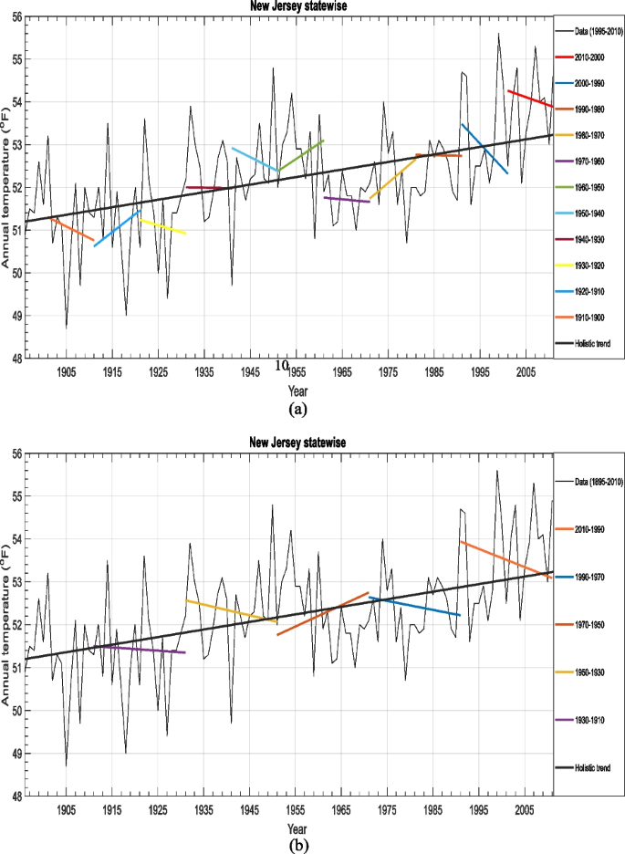

New Jersey annual temperature trends, a 10-year, b 20-year, c 30-year, d 40-year


In Fig. 4 all period moving average trends are shown collectively, which shows that whatever is the moving trend period there is in all increasing trend position irrespective of increasing or decreasing tendency. Although there appear decreasing moving trends in the most recent periods compared to the same set moving trend position is in increase.

New Jersey State wise temperature records moving trend collection
Annual precipitation records of Istanbul City from 1940 to 2012 are shown in Fig. 5 with moving trend components over each periods. The overall trend tends to increase with slope 0.0507 cm/year, which means a very small increase in precipitation record moving means.
-
1)
For 10-year moving trends below the overall trend indicates possible water shortages that have occurred at various time durations in the past and it is clear from Fig. 5a that decadal shortages are about 86% (see Fig. 5a). The only decade with increasing precipitation seems from 1962 to 1972,
-
2)
20-year moving trends during 1972–1992 and 1992–2002 periods are the same with the holistic trend that shows quite stationary rainfall regime on the average in the last 40 years of the record,
-
3)
As for the 30-year period during 1982–2002 there appears a slight decrease around the holistic trend. The middle point position of this moving trend lies on the holistic trend line. This means that during the first (second) half of this period moving trend decrease is above (below) the holistic trend (see Fig. 5c),
-
4)
Figure 5d is for 40-year period decreasing moving trend component, which has almost the same slope as the holistic trend again with half slightly over and the next half below the holistic trend.
Fig. 5 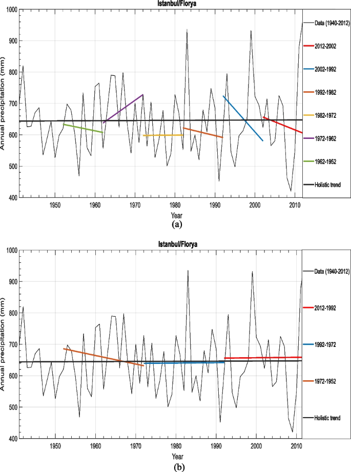
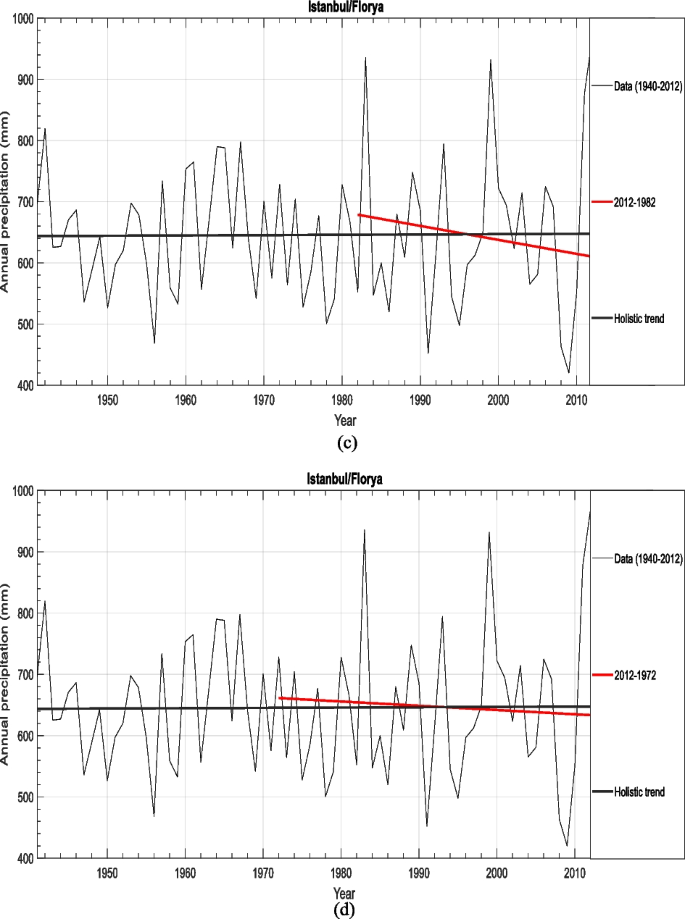
Istanbul annual precipitation trends, a 10-year, b 20-year, c 30-year, d 40-year


Moving trends of different periods are shown collectively in Fig. 6, where only 10-year period moving trends expose quite sharp increasing and decreasing trends. Especially, the last 30-year trend indicates a decreasing trend of which the middle point lies on the holistic trend with early (late) half is above (below) the holistic trend.

Istanbul/Florya precipitation records moving trend collection
A set of slope values for moving trends are given in Table 2 for each data set including different periods 10-year, 20-year, 30-year and 40-year, respectively. A wide variety of moving trend slope variations can be noticed for each period. The mean and the standard deviations of each period are also given in the same table.
Of course, the average values are based on positive (increasing) and negative (decreasing) trend values and thus generally show the general trend towards overall positive or negative moving trend values. A common point as for the 30-year period is concerned that all the hydro-meteorology records have decreasing trend slopes. For example, Istanbul moving trend average values are negative for all periods, indicating that it is possible to expect precipitation reduction in future time periods.
5 Discussion
There are different trend identification methodologies in the open literature and some of them require restrictive assumptions that are not very satisfactory for natural hydro-meteorological recording time series, for which the assumption of serial independence is most important. Some are interested in non-parametric procedures in which the natural order of hydro-meteorology time series is replaced, for example, by orders as ranks (Spearman 1904). Most of these trending tests require long time series as their results are in biased for short samples. In this article, innovative trend analysis (ITA) methodology is applied as a different approach to overall trend determination, because moving trend components are valid even for time series samples that are significantly shorter than the World Meteorology Organization recommendation of 30 years (WHO 2017). Overwhelmingly, theoretical trend identification or practical procedures predominantly consider the entire sample length of a given time series. Many are biased because they do not meet key constraining assumptions such as serial independence, normal (Gaussian) probability distribution function (PDF) or long sample lengths.
Comparing the results of MTM procedure for different sub-periods of a hydro-meteorology time series provides the dynamic behavior of finite length trend development over the recording period. Generally, moving trends fluctuate around the overall trend line. Comparing up and down moving trend numbers to understand the frequency of short-term percentages result in higher (lower) values than the overall trend. Instead of taking future action according to the overall full recording time trend, making dynamic comments considering the sequence of MTM trends, and accordingly, better trending probability in the future.
The innovative aspect of this paper is the dynamic description of the desired partial-time trend analysis instead of holistic classical trend trends that do not show cycles of increasing and decreasing trend evolution over the entire length of the record. Once possible finite-term trend slopes have been identified, it is possible to make same-term future trend slope forecasts for improved water resources management planning and operation.
The MTM methodology provides information about trend slopes, so that during which moving trend duration the maximum and minimum increasing and decreasing slopes occur and, if necessary, average slopes for these two types of trends can be determined.
6 Conclusions
As a result of the greenhouse gas (GHG) emissions into the troposphere, global warming has led to climate change at different increasing or decreasing rates in different parts of the world. In climate change impact studies, trend analysis procedures are important to decide whether there is an increasing or decreasing overall trend for a hydro-meteorological variable at a location, unlike general circulation (climate) models (GCMs). This paper provides moving trend analysis for several sub-periods in a given time series records and their comparison with classical holistic trend procedures in the literature. For this purpose, a dynamic trend evaluation study is carried out by investigating subsequent special moving trend for 10-year, 20-year, 30-year and 40-year periods. The application of the proposed moving trend methodology is given for annual records of Danube River discharges, New Jersey state-wise temperatures and Istanbul City precipitation. Moving trending also provides percentages of decreasing (increasing) trend activity over the entire time series. It is recommended that the application of moving trend analysis sheds light on more dynamic structural behavior of hydro-meteorological records. The only limitation for holistic trend analysis is at least 30 years of data, which is recommended by the World Meteorological Organization and is also valid for the moving trend analysis methodology. There has not been yet any other research using MTM analysis, but in future water resources management studies such part-time trends tend to provide important information about dry and wet trend tendencies and their likely duration.
Data Availability
Data can be provided upon request from the corresponding author.
References
Abbas M, Arshad M, Shahid MA (2023) Zoning of groundwater level using innovative trend analysis: case study at Rechna Doab, Pakistan. Water Resour Irrig Manage - WRIM 12:64–80. https://doi.org/10.19149/wrim.v12i1-3.3155
Achite M, Ceribasi G, Ceyhunlu AI et al (2021) The innovative polygon trend analysis (IPTA) as a simple qualitative method to detect changes in Environment—Example detecting trends of the total monthly precipitation in semiarid area. Sustainability 13:12674. https://doi.org/10.3390/su132212674
Alashan S (2018) An improved version of innovative trend analyses. Arab J Geosci 11(3):50
Ashraf MS, Ahmad I, Khan NM, Zhang F, Bilal A, Guo J (2021) Streamflow variations in monthly, seasonal, annual and extreme values using Mann-Kendall, Spearmen’s rho and innovative trend analysis. Water Resour Manag 35:243–261
Birpınar ME, Kızılöz B, Şişman E (2023) Classic trend analysis methods’ paradoxical results and innovative trend analysis methodology with percentile ranges. Theor Appl Climatol. https://doi.org/10.1007/s00704-023-04449-6
Box GEP, Jenkins GM (1976) Time series analysis, forecasting and control. Holden-Day, San Francisco
Burn DH, Hag Elnur MA (2002) Detection of hydrologic trends and variability. J Hydrol 255:107–122
Cailas MD, Cavadias G, Gehr R (1986) Application of a non-parametric approach for monitoring and detecting trends in water quality data of the St. Lawrence River. Water Pollut Res J Can 21(2):153–167
Demaree GR, Nicolis C (1990) Onset of Sahelian drought viewed as a fluctuation-induced transition. Q J R Meteorol Soc 116:221–238
Douglas EM, Vogel R, Kroll CN (2000) Trends in floods and low flows in the United States: impact of spatial correlation. J Hydrol 240:90–105
Esit M, Kumar S, Pandey A et al (2021) Seasonal to multi-year soil moisture drought forecasting. Clim Atmospheric Sci 4:1–8. https://doi.org/10.1038/s41612-021-00172-z
Fanta SS, Yesuf MB, Saeed S et al (2022) Analysis of precipitation and temperature trends under the impact of climate change over ten districts of Jimma Zone, Ethiopia. Earth Syst Environ. https://doi.org/10.1007/s41748-022-00322-0
Gan TY (1998) Hydro-climatic trends and possible climatic warming in the Canadian prairies. Water Resour Res 34(11):3009–3015
Güçlü YS (2018) Multiple Şen-innovative trend analyses and partial Mann-Kendall test. J Hydrol Elsevier 566:685–704
Hamed KH (2008) Trend detection in hydrologic data: the Mann–Kendall trend test under the scaling hypothesis. J Hydrol 349:350–363
Hamilton JP, Whitelaw GS, Fenech A (2001) Mean annual temperature and annual precipitation trends at Canadian biosphere reserves. Environ Monit Assess 67:239–275
Hipel KW, McLeod AI, Weiler RR (1988) Data analysis of water quality time series in Lake Erie, Water Resour. Bull 24(3):533–544
Hirca T, Eryılmaz TG, Niazkar M (2022) Applications of innovative polygonal trend analyses to precipitation series of Eastern Black Sea Basin, Turkey. Theor Appl Climatol 147:651–667. https://doi.org/10.1007/s00704-021-03837-0
Hirsch RM, Slack JR (1984) A nonparametric trend test for seasonal data with serial dependence. Water Resour Res 20(1):727–732
Hirsch RM, Slack JR, Smith RA (1982) Techniques of trend analysis for monthly water quality analysis. Water Resource Res 18(1):107–121
IPCC (2007) Climate Change 2007: impacts, adaptation, and vulnerability. Contribution of Working Group II to the Fourth Assessment Report of the Intergovernmental Panel on Climate Change. Cambridge University Press, Cambridge
Kalra A, Piechota TC, Davies R, Tootle GA (2008) Changes in U.S. streamflow and western U.S. snowpack. J Hydrol Eng 13:156–163
Kendall MG (1970) Rank correlation methods, 4th edn. Griffin, London
Kendall MG (1973) Rank correlation methods. Charles Griffin Book Series, London
Lee H, Apley DW (2011) Improved design of robust exponentially weighted moving average control charts for autocorrelated processes. Qual Reliab Eng Int 27(3):337–352
Lins HF, Slack JR (1999) Streamflow trends in the United States. Geophys Res Lett 26(2):227–230
Mann HB (1945) Nonparametric tests against trend. Econometrica 13(3):245–259
Mann HB (1955) Non-parametric tests against trend Econometrica. J Econom Soc 13(3):245–259
Mateus C, Potito A (2022) Long-term trends in daily extreme air temperature indices in Ireland from 1885 to 2018. Weather Clim Extrem 36:100464
Milly PCD, Betancourt J, Falkenmark M, Hirsch RM, Kundzewicz ZW, Lettenmaier DP, Stouffer RJ (2008) Stationarity is dead: whither water management? Science 319:573–574
O’Brien NL, Burn DH, Annable WK, Thompson PJ (2021) Trend detection in the presence of positive and negative serial correlation: a comparison of block maxima and peaks-over-threshold data. Water Resour Res 57:e2020WR028886
Pastagia J, Mehta D (2022) Application of innovative trend analysis on rainfall time series over Rajsamand district of Rajasthan state. Water Supply 22:7189–7196. https://doi.org/10.2166/ws.2022.276
Sen PK (1968) Estimates of the regression coefficient based on Kendall’s tau. J Am Stat Assoc 63(324):1379–1389
Şen Z (2012) Innovative trend analysis methodology. J Hydrol Eng 17(9):1042–1046
Şen Z (2017) Hydrological trend analysis with innovative and over-whitening procedures. Hydrol Sci J 62(2):294–305
Sonali P, Kumar DN (2013) Review of trend detection methods and their application to detect temperature changes in India. J Hydrol 476:212–227
Spearman C (1904) The proof and measurement of association between two things. Am J Psychol 15:72–101. https://doi.org/10.2307/1412159
Taylor CH, Loftis JC (1989) Testing for trend in lake and groundwater quality time series. Water Resour Bull 25(4):715–726
Ullah I, Ma X, Yin J, Omer A, Habtemicheal BA, Saleem F, Iyakaremye V, Syed S, Arshad M, Liu M (2022) Spatiotemporal characteristics of meteorological drought variability and trends (1981–2020) over South Asia and the associated large-scale circulation patterns. Clim Dyn 60:2261–2284
Van Belle VG, Hughes JP (1984) Nonparametric tests for trends in water quality. Water Resour Res 20(1):127–136
WHO (2017) WMO Guidelines on the Calculation of Climate Normals. WMO-No. 1203. p 18
Xie Y, Liu S, Huang S, Fang H, Ding M, Huang C, Shen T (2022) Local trend analysis method of hydrological time series based on piecewise linear representation and hypothesis test. J Clean Prod 339:130695
Yeh AB, Lin DK, Zhou H, Venkataramani CH (2003) A multivariate exponentially weighted moving average control chart for monitoring process 52 variability. J Applied Statistics 30(5):507–536
Yu YS, Zou S, Whittemore D (1993) Non-parametric trend analysis of water quality data of river in Kansas. J Hydrol 150:61–80
Yue S, Wang CY (2002) Applicability of pre-whitening to eliminate the influence of serial correlation on the Mann-Kendall test. Water Resour Res 38. https://doi.org/10.1029/2001WR000861
Funding
Open access funding provided by the Scientific and Technological Research Council of Türkiye (TÜBİTAK). The research received no funds.
Author information
Authors and Affiliations
Contributions
All parts are contributed by the single author.
Corresponding author
Ethics declarations
Ethical Approval
The manuscript is conducted in the ethical manner advised by the targeted journal.
Consent to Participate
Not applicable.
Consent to Publish
The research is scientifically consented to be published.
Conflict of Interest
The author declares no conflict of interest to any party.
Additional information
Publisher’s Note
Springer Nature remains neutral with regard to jurisdictional claims in published maps and institutional affiliations.
Rights and permissions
Open Access This article is licensed under a Creative Commons Attribution 4.0 International License, which permits use, sharing, adaptation, distribution and reproduction in any medium or format, as long as you give appropriate credit to the original author(s) and the source, provide a link to the Creative Commons licence, and indicate if changes were made. The images or other third party material in this article are included in the article's Creative Commons licence, unless indicated otherwise in a credit line to the material. If material is not included in the article's Creative Commons licence and your intended use is not permitted by statutory regulation or exceeds the permitted use, you will need to obtain permission directly from the copyright holder. To view a copy of this licence, visit http://creativecommons.org/licenses/by/4.0/.
About this article

Cite this article
Şen, Z. Moving Trend Analysis Methodology for Hydro-meteorology Time Series Dynamic Assessment. Water Resour Manage (2024). https://doi.org/10.1007/s11269-024-03872-2
Received:
Accepted:
Published:
DOI: https://doi.org/10.1007/s11269-024-03872-2