Diffuse Radio Emission from Galaxy Clusters

Abstract

In a growing number of galaxy clusters diffuse extended radio sources have been found. These sources are not directly associated with individual cluster galaxies. The radio emission reveal the presence of cosmic rays and magnetic fields in the intracluster medium (ICM). We classify diffuse cluster radio sources into radio halos, cluster radio shocks (relics), and revived AGN fossil plasma sources. Radio halo sources can be further divided into giant halos, mini-halos, and possible “intermediate” sources. Halos are generally positioned at cluster center and their brightness approximately follows the distribution of the thermal ICM. Cluster radio shocks (relics) are polarized sources mostly found in the cluster’s periphery. They trace merger induced shock waves. Revived fossil plasma sources are characterized by their radio steep-spectra and often irregular morphologies. In this review we give an overview of the properties of diffuse cluster radio sources, with an emphasis on recent observational results. We discuss the resulting implications for the underlying physical acceleration processes that operate in the ICM, the role of relativistic fossil plasma, and the properties of ICM shocks and magnetic fields. We also compile an updated list of diffuse cluster radio sources which will be available on-line (http://galaxyclusters.com). We end this review with a discussion on the detection of diffuse radio emission from the cosmic web.

1 Introduction

Galaxy clusters are the largest virialized objects in our Universe, with masses up to $\sim 10^{15}~\mbox{M}_{\odot }$. Elongated filaments of galaxies, located between clusters, form even larger unbound structures, making up the cosmic web. Galaxy clusters are located at the nodes of filaments, like “spiders” in the cosmic web.

Clusters contain up to several thousands of galaxies. However, the galaxies comprise only a few percent of a cluster’s total mass. Most of the baryonic mass of clusters is contained in a hot ($10^{7}$–$10^{8}$ K) ionized intracluster medium (ICM), held together by the clusters’ gravitational pull. This dilute magnetized plasma ($\sim 10^{-3}~\text{particles~cm}^{-3}$) emits thermal Bremsstrahlung at X-ray wavelengths, permeating the cluster’s volume (e.g., Mitchell et al. 1976; Serlemitsos et al. 1977; Forman and Jones 1982), see Fig. 1. The ICM makes up ∼15% of a cluster’s mass budget. Most of the mass, $\sim 80\%$, is in the form of dark matter (e.g., Blumenthal et al. 1984; White and Fabian 1995; Jones and Forman 1999; Arnaud and Evrard 1999; Sanderson et al. 2003; Vikhlinin et al. 2006).

Fig. 1

The galaxy cluster Abell 2744. The left panel shows an optical (Subaru BRz; Medezinski et al. 2016) view of the cluster. White linearly spaced contours represent the mass surface density ($\kappa$) derived from a weak lensing study ($\kappa = {\varSigma }/{\varSigma _{\mathrm{{cr}}}}$, with $\varSigma _{(\mathrm{cr})}$ the (critical) mass surface density) overlaid from Merten et al. (2011), Lotz et al. (2017). In the middle panel the X-ray emission from the thermal ICM (Chandra 0.5–2.0 keV band) is displayed in blue. In the right panel a 1–4 GHz Very Large Array (VLA) image is shown in red, tracing cosmic rays and magnetic fields. For more details about the images see Pearce et al. (2017)

Elongated filaments of galaxies span the regions between clusters. The so-called warm-hot intergalactic medium (WHIM) pervades these galaxy filaments (Cen and Ostriker 1999). Compared to the ICM, the intergalactic medium of galaxy filaments (WHIM) has a significantly lower density ($\lesssim 10^{-4}~\text{particles cm}{-3}$) and cooler temperature ($10^{5}$–$10^{7}$ K). About half of the Universe’s baryons reside in this WHIM (e.g., Cen and Ostriker 1999; Davé et al. 2001; Eckert et al. 2015). Galaxy filaments are expected to be surrounded by strong accretion shocks, where the plasma is first shock-heated (Sunyaev and Zeldovich 1972). However, studying the WHIM and associated shocks is difficult due to a lack of sensitive observational tools. Galaxy clusters form by accretion from the WHIM and through a sequence of mergers of clusters and groups (e.g., Peebles and Yu 1970; Press and Schechter 1974; Voit 2005; Kravtsov and Borgani 2012). Cluster mergers are very energetic events, releasing energies up to $\sim 10^{64}$ ergs on a few Gyr timescale. This energy is dissipated through low-Mach number shocks and turbulence, heating the ICM (e.g., Markevitch and Vikhlinin 2007). Clusters can thus be divided as either “relaxed” (undisturbed) or “merging” (disturbed) systems, depending on their dynamical (merging) state.

Galaxy clusters often host a number of active galactic nuclei (AGN) that emit radio synchrotron emission (i.e., radio galaxies) (e.g., De Young 1984; de Young 2002; Tadhunter 2016). The sizes of these sources range from a few kpc to about ∼1 Mpc, extending well beyond the host galaxy. A major difference with radio galaxies that are located outside clusters (and groups) is that the jets and lobes of cluster radio galaxies often show signs of interaction with the ICM (e.g., Miley 1980; Burns 1998; Johnston-Hollitt et al. 2015a). These interactions result in morphologies that range from wide-angle (WAT), narrow angle (NAT), to “head-tail” radio sources.

Gas in the central regions of many relaxed clusters has a radiative cooling time that is much shorter than the Hubble time. In the absence of a heating source, a cooling flow is expected to develop, whereby the temperature in the central region of the cluster drops and gas flows inwards (e.g., Fabian 1994, 2012; Peterson and Fabian 2006; McNamara and Nulsen 2012). X-ray observations do show these temperature drops in some cluster cores (“cool core” clusters), but there is much less cool gas than what would be expected from the short radiative cooling time (Kaastra et al. 2001; Peterson et al. 2001, 2003). Therefore, some source of heating must balance the radiative losses. Radio galaxies, associated with the brightest cluster galaxy (BCG), have been identified as the main source of energy input into the ICM. X-ray observations show numerous cavities in cool core clusters, coincident with the lobes of the central radio galaxy. Here the radio plasma has displaced the X-ray emitting gas, creating a low-density bubble which rises buoyantly and expands, distributing energy to the surrounding ICM (e.g., Churazov et al. 2002). This process is commonly referred to as “radio-mode” feedback, although it is still being debated what the precise mechanism is that transfers the energy to the ICM.

1.1 Extended Synchrotron Radio Emission from Galaxy Clusters

Radio observations have shown that the ICM can also contain a non-thermal component of cosmic rays (CR, see Fig. 1) which is not directly associated with cluster radio galaxies (e.g., Large et al. 1959; Willson 1970). These GeV CR electrons (i.e., Lorentz factors of $\gamma > 10^{3}$) emit synchrotron radiation in the presence of ∼μGauss ICM magnetic fields. During the last decade significant progress has been made in our understanding of this non-thermal component, through observations, theoretical, and numerical work. There is now compelling evidence that ICM shocks waves, and likely also turbulence, are able to (re-)accelerate particle to relativistic energies creating this non-thermal CR component of the ICM.

The presence of extended synchrotron emission also indicates the existence of large-scale ICM magnetic fields with a strength of the order of 0.1–10 μGauss (e.g., Brüggen et al. 2012; Clarke et al. 2001; Johnston-Hollitt et al. 2015b). Cluster magnetic fields play an important role in particle acceleration processes. Additionally, magnetic fields inhibit transport processes like heat conduction, spatial mixing of gas, and the propagation of cosmic rays (e.g., Pfrommer et al. 2017; Ruszkowski and Oh 2010). However, few details are known about the precise properties of these fields since they are difficult to measure (e.g., Govoni and Feretti 2004).

The synchrotron emitting CR electrons should scatter photons from the cosmic microwave background (CMB) to X-ray energies, resulting in a hard tail on top of the thermal X-ray spectrum of clusters (Rephaeli 1979; Rephaeli et al. 1994; Sarazin and Kempner 2000). So far, no conclusive detection of this inverse-Compton (IC) radiation has been made (e.g., Fusco-Femiano et al. 2000, 2001; Rephaeli and Gruber 2004; Rossetti and Molendi 2004; Fusco-Femiano 2004; Rephaeli et al. 2008; Eckert et al. 2008; Wik et al. 2009, 2014). However, even a non-detection of IC X-ray emission, in combination with radio observations, is useful to set lower limits on the ICM magnetic fields strength (e.g., Sugawara et al. 2009; Finoguenov et al. 2010; Itahana et al. 2015). Similarly, CR protons can interact hadronically with the protons of the ICM and generate pions that can then decay into gamma-rays (cf., Dennison 1980; Blasi and Colafrancesco 1999; Blasi et al. 2007). Gamma-ray observations are particularly important to understand the dynamical role of CR protons in clusters, and the role of secondary electrons, also coming from pion decays, in generating the extended radio emission.

1.2 This Review

Galaxy clusters provide a unique environment to study the physics of particle acceleration in collisionless, high-$\beta$, turbulent plasmas, where $\beta$ is the ratio of the thermal pressure to the magnetic pressure,¹ and at low Mach numbers shocks. Furthermore, diffuse radio emission from clusters can be used as a signpost of ICM shocks and turbulence, which are often difficult to detect and characterize at other wavelengths. Since shocks and turbulence trace the dynamical state of the ICM, radio observations also provide us with a probe of the cluster’s evolutionary stage, important for our understanding of structure formation in the Universe. Finally, diffuse radio emission can be used as a complementary method to discover clusters that were missed by X-ray, SZ, or optical surveys (Brown et al. 2011a; van Weeren et al. 2012b; Macario et al. 2014; de Gasperin et al. 2017b).

In this paper we review the observational properties of diffuse extended cluster radio emission. Previous observational reviews on this subject were presented by Feretti (2002, 2003), Giovannini and Feretti (2002), Ferrari et al. (2008), Feretti et al. (2012). Here we provide an update, encompassing recent results that have helped to improve our understanding of these sources. For a more theoretical review we refer the reader to Brunetti and Jones (2014). Observational progress in this field has been made through a combination of high-resolution multi-frequency studies, the availability of deep low-frequency observations, an increasing number of polarimetric studies, the compilation of larger cluster samples with deep radio data, and high-frequency detections. The joint analyses of radio data and observations at other wavelengths, in particular in the X-ray and Gamma-ray bands, has also played an important role.

The outline of this paper is as follows. In Sect. 2 we briefly discuss synchrotron radiation and particle acceleration mechanisms. The classification of diffuse cluster radio sources is discussed in Sect. 3. A review of cluster magnetic fields is given in Sect. 4. Overviews of radio halos, including mini-halos, and cluster radio shocks and revived fossil plasma sources are presented in Sects. 5 and 6. In Sect. 7 we end this review with a discussion on the detection of diffuse radio emission outside cluster environments.

2 Synchrotron Radiation and Radio Spectra

In this section we briefly discuss some relevant theory about the synchrotron spectra of CR electrons. For a more detailed treatment of synchrotron radiation we refer the reader to the references provided in Feretti et al. (2012). A standard assumption is that the ICM CR population can be described by a power law energy ($E$) distribution

$$ n(E)\mathrm{d} E \propto E^{-p} \mathrm{d} E . $$

(1)

The index of the energy (or momentum) distribution $p$ is directly related to the radio spectral index²

$$ p=1\mbox{--}2\alpha . $$

(2)

Diffuse cluster radio emission typically has a steep spectral index, i.e., $\alpha \lesssim -1$. The spectral shape is related to the physics of the acceleration mechanism and the electron synchrotron and IC energy losses. The characteristic lifetime ($t_{\mathrm{age}}$) of the synchrotron emitting electrons ($\gamma \sim 10^{4}$; GeV energy) due to these energy losses is

$$ t_{\mathrm{age}}~\mbox{[yr]} \approx 3.2 \times 10^{10} \frac{B^{1/2}}{B ^{2} + B^{2}_{\mathrm{CMB}}} \bigl[(1+z)\nu \bigr]^{-1/2}, $$

(3)

where $B$ the magnetic field strength, $z$ the source redshift, $B_{\mathrm{CMB}}$ the equivalent magnetic field strength of the CMB ($B _{\mathrm{CMB}} \ [\upmu \text{Gauss}] \approx 3.25 (1+z ) ^{2}$), and $\nu$ the observing frequency in MHz. In clusters, we have $t_{\mathrm{age}} \lesssim 10^{8}$ yrs. The typical diffusion length-scale in the ICM of a GeV electron, using the Bohm approximation, is of the order of 10 pc (e.g., Bagchi et al. 2002). Plasma motions can increase the distance over which GeV electrons travel, but this distance is still expected to remain well below a Mpc. This means that Mpc-scale diffuse radio sources cannot trace CR electrons that are accelerated at a single location in the ICM. Instead, they need to be (re-)accelerated or produced in-situ (Jaffe 1977), providing important constraints on the possible acceleration/production mechanisms.

Due to the energy losses, the initial power-law spectrum steepens beyond a break frequency, whose position is related to the time since acceleration. The power-law spectrum is commonly refereed to as the injection spectrum, characterized by an injection spectral index ($\alpha _{\mathrm{{inj}}}$). For the JP (Jaffe-Perola) synchrotron spectrum (Jaffe and Perola 1973), one assumes that there is a continuous isotropization of the electron pitch angles (i.e., angle between the magnetic field and the electron velocity) on a timescale that is shorter than $t_{\mathrm{age}}$. A JP spectrum describes a synchrotron spectrum from a single burst of acceleration and then aging. The KP (Kardashev-Pacholczyk) model (Kardashev 1962; Pacholczyk 1970) also represents such a spectrum, but without the isotropization of the pitches angles. A collection of spectral shapes is displayed in Fig. 2.

Fig. 2

An overview of radio spectral shapes. All spectral models have $\alpha _{\mathrm{{inj}}} = -0.6$. The power-law spectrum depicts the spectral shape before any energy losses

Since it is usually difficult to spatially isolate electrons that all have the same spectral age, there are also composite models. These models sum JP (or KP) spectra with different amounts of spectral aging. The CI (continuous injection) composite model (Pacholczyk 1970) describes the integrated spectrum of a source with continuous particle injection. For the KGJP/KGKP (Komissarov-Gubanov) model (Komissarov and Gubanov 1994), the particles are only injected for a finite amount of time before the injection in the source stops.

2.1 Particle Acceleration Mechanisms

There are several physical mechanisms to accelerate particles in the ICM and produce the synchrotron emitting CR electrons. We briefly give an overview of these processes below. Further details will be discussed in later sections where relevant.

• First order Fermi acceleration (Fermi-I): This process, also known as diffusive shock acceleration (DSA), plays an important role in various astrophysical environments (Krymskii 1977; Axford et al. 1977; Bell 1978a,b; Blandford and Ostriker 1978; Drury 1983; Blandford and Eichler 1987; Jones and Ellison 1991; Malkov and O’C Drury 2001). For DSA, particles are accelerated at a shock with the acceleration taking place diffusively. In this process, particles cross back and forward across the shock front as they scatter from magnetic inhomogeneities in the shock down and upstream region. At each crossing, particles gain additional energy, forming a power-law energy distribution of CR.

• Second order Fermi acceleration (Fermi-II): This is a stochastic process where particles scatter from magnetic inhomogeneities, for example from magneto-hydrodynamical (MHD) turbulence (Schlickeiser et al. 1987; Schlickeiser and Achatz 1993; Brunetti et al. 2001; Petrosian 2001). Particles can either gain or loose energy when scattering. When the motions are random, the probability for a head-on collision, where energy is gained, is slightly larger. Because of its random nature, second order Fermi acceleration is an inefficient process.

• Adiabatic compression: A shock wave can adiabatically compress a bubble/lobe/cocoon of (old) relativistic radio plasma from an AGN. Due to the compression, the CR electrons in the cocoon regain energy boosting the radio synchrotron emission (Enßlin and Gopal-Krishna 2001; Enßlin and Brüggen 2002).

• Secondary models: Another mechanism to produce CR electrons is via a secondary process, meaning that the CR electrons are produced as secondary particles (decay products). In the hadronic model, collisions between relativistic protons and the thermal ions produce secondary CR electrons (Dennison 1980; Blasi and Colafrancesco 1999; Dolag and Enßlin 2000; Miniati et al. 2001a; Keshet and Loeb 2010; Donnert et al. 2010; Enßlin et al. 2011). Since CR protons have a very long lifetime compared to CR electrons, they will accumulate over the lifetime of a cluster once they are accelerated. Possible mechanisms to produce CR protons are first order Fermi acceleration at shocks, AGN activity, and galactic outflows (supernovae, winds).

3 Classification

Diffuse cluster radio sources have historically been divided into three main classes, relics, halos, and mini-halos (Feretti and Giovannini 1996). In addition, radio filaments were proposed to trace the large-scale filaments of the cosmic web, outside of clusters. Note that the term filament has also sometimes been used to describe radio relics (or relic-type structures) in clusters. We will discuss radio emission outside the cluster environment in Sect. 7.

Radio halos are centrally located diffuse sources in merging clusters. They do not have any optical counterparts. Mini-halos have smaller sizes and are located in relaxed cool core clusters which also host a powerful radio galaxy associated with the BCG. Radio relics have been defined as extended sources that show high levels of polarization ($\gtrsim 10\%$ at GHz frequencies) and are located in the cluster periphery. Similar to radio halos, they not show optical counterparts. Relics were further subdivided (Kempner et al. 2004) into large Radio Gischt, large Mpc-size sources that trace particles accelerated at shocks via Fermi-I processes; Radio Phoenices, AGN fossil plasma compressed and revived by merger shocks; and AGN Relics, fossil radio plasma that is passively evolving from an AGN that has been switched off. For radio relics, the boundaries between the different categories is not always very obvious and the term relics itself is somewhat unfortunate because large relics could be “young” sources with on-going (re-)acceleration.

Here we propose to classify cluster emission into three broad classes:

• Radio halos are extended sources that roughly follow the ICM baryonic mass distribution. This class includes giant radio halos and mini-halos, see Fig. 3. This class would also contain possible “intermediate” or “hybrid” radio halos, with properties falling somewhere in between those of classical giant radio halos and mini-halos. Another property of the halo class is that these sources are not localized, in the sense that particle (re-)acceleration/production occurs throughout a significant volume of the cluster and is not associated with a particular shock which location can be pint-pointed. In terms of a physical interpretation, these “global” sources should trace Fermi-II processes and/or secondary electrons.

  Fig. 3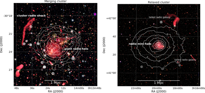

  

  Left panel: VLA 1–4 GHz image of the merging galaxy cluster Abell 2744 with different source classes labeled (see also Fig. 1). Chandra X-ray contours are shown in white. This cluster hosts a luminous giant radio halo and a cluster radio shock (relic). X-ray surface brightness contour are drawn proportional to $[1,4,16,64,\ldots ]$. Right panel: VLA 230–470 MHz image of the relaxed cool core Perseus cluster from Gendron-Marsolais et al. (2017). XMM-Newton X-ray contours in the 0.4–1.3 keV band are overlaid in white with the same contour spacing as in the left panel. The Perseus cluster hosts a radio mini-halo as well as two prominent tailed radio galaxies

• Cluster radio shocks (radio relics) are extended diffuse sources tracing particles that are (re-)accelerated at ICM shock waves (Fig. 3). They have commonly been referred to as radio relics. This radio shock classification is somewhat similar to the that of Gischt, but it does not necessarily require DSA or Fermi-I type acceleration. In that sense, cluster radio shocks are an observationally defined class, unrelated to the details of the actual acceleration mechanism. However, based on our current understanding of these sources, we do anticipate that in most cases cluster radio shocks are associated with Fermi-I acceleration processes. It is not required that cluster radio shocks are located in the cluster periphery, although for large cluster radio shocks that will typically be the case. Due to their nature, the large majority of these sources are expected to show a high degree of polarization. Sources previously classified as large radio relics, Gischt, and double relics, fall in the cluster radio shock category. Unlike radio halos, cluster radio shocks can be associated to a specific cluster region where a shock wave is present, or where a shock wave recently passed. A drawback of the radio shock classification is that the detection of shocks in the ICM is observationally challenging. Therefore, the classification will remain uncertain for some sources. However, for a number of sources the presence of a shock at their location has been confirmed by X-ray observations (see Sect. 6.1.5) which we argue warrants the creation of a radio shock class. In this review we will use the term radio shock for sources previously classified as large radio relics, Gischt, and double relics. It is important to keep in mind that for a number of sources the presence of a shock remains to be confirmed.

• Revived AGN fossil plasma sources, phoenices, and GReET In this class we group sources that trace AGN radio plasma that has somehow been re-energized through processes in the ICM, unrelated to the radio galaxy itself. Low-frequency observations are starting to reveal more and more of these type of sources. However, their precise origin and connection to cluster radio shocks and possibly also halos is still uncertain. The main observational property that the sources have in common is the AGN origin of the plasma and their ultra-steep radio spectra due to their losses. For this review we decided to keep the radio phoenix classification (Kempner et al. 2004). Often these phoenices display irregular filamentary morphologies. They have relatively small sizes of at most several hundreds of kpc. Gently re-energized tails (GReETs; de Gasperin et al. 2017a) are tails of radio galaxies that are somehow revived, showing unexpected spectral flattening, opposite from the general steepening trend caused by electron energy losses. With the new and upgraded low-frequency radio telescopes that have become operational, we expect that the nature of these revived fossil plasma sources will become more clear over the next decade.

Fossil radio plasma plays and important role in some of the models for the origin of radio halos and cluster radio shocks. In these models fossil plasma is re-accelerated via first and second order Fermi processes. This implies that when clusters are observed at low enough frequencies, both halos and cluster radio shocks will blend with regions of old AGN radio plasma, complicating the classification.

The classification can also be hindered by projection effects. For example, a cluster radio shock observed in front of the cluster center might mimic halo-type emission if the signal to noise of the image is not very high. However, these are observation related difficulties, which can in principle be resolved with better data. On the website http://galaxyclusters.com we provide an up to date list of the currently known diffuse cluster radio sources and their classification. An up-to-date list of clusters with (candidate) diffuse radio emission at the time of writing (September 2018) is shown in Table 1.

Table 1 Clusters with diffuse radio emission

4 Cluster Magnetic Fields

4.1 Global

Magnetic fields permeate galaxy clusters and the intergalactic medium on Mpc-scales. These fields play key roles in particle acceleration and on the process of large scale structure formation, having effects on turbulence, cloud collapse, large-scale motions, heat and momentum transport, convection, viscous dissipation, etc. In particular, cluster magnetic fields inhibit transport processes like heat conduction, spatial mixing of gas, and propagation of cosmic rays. The origin of the fields that are currently observed remains largely uncertain. A commonly accepted hypothesis is that they result from the amplification of much weaker pre-existing seed fields via shock/compression and/or turbulence/dynamo amplification during merger events and structure formation, and different magnetic field scales survive as the result of turbulent motions (e.g., Kahniashvili et al. 2013). The origin of seed fields is unknown. They could be either primordial, i.e., generated in the early Universe prior to recombination, or produced locally at later epochs of the Universe, in early stars and/or (proto)galaxies, and then injected in the interstellar and intergalactic medium (Rees 2006). For a review about magnetic field amplification in clusters we refer the reader to Donnert et al. (2018).

Magnetic fields are difficult to measure. Some estimates have relied on the idea that the energies in cosmic rays and magnetic fields in the radio emitting regions are the same (“equipartition”; Beck and Krause 2005). In this way, magnetic field values in the range 0.1–10 μGauss are obtained. However, this method is inherently uncertain due to the many assumptions that are required. Cosmological simulations of clusters predict μGauss-level magnetic field strengths in the cluster centers and a decrease of the magnetic field strength with radius in the outer regions (Dolag et al. 1999, 2001, 2002; Vazza et al. 2014, 2018). These values are roughly consistent with equipartition magnetic field strengths estimates of the order of a μGauss.

The most promising technique to derive a more detailed view of the magnetic fields in clusters is via the analysis of the Faraday rotation of radio galaxies located inside and behind the cluster (e.g., Clarke 2004; Govoni and Feretti 2004). Faraday rotation changes the intrinsic polarization angle ($\chi _{0}$). The Faraday depth ($\phi$) is related to the properties of the plasma that cause the Faraday rotation (Burn 1966; Brentjens and de Bruyn 2005)

$$ \phi (\mathbf{r}) = 0.81 \int _{\mathrm{source}}^{\mathrm{telescope}} n _{\mathrm{e}}\mathbf{B} \cdot \, d\mathbf{r} \mbox{ } \bigl[\mbox{rad}\,\mbox{m} ^{-2} \bigr] , $$

(4)

where $n_{\mathrm{e}}$ is the electron density in units of $\text{cm}^{-3}$, $\mathbf{B}$ the magnetic field in units of μGauss, and $d\mathbf{r}$ is an infinitesimal path length in along the line of sight in units of parsec. The rotation measure (RM) is defined as

$$ \mathrm{RM} = \frac{d\chi (\lambda ^{2})}{d\lambda ^{2}}, $$

(5)

where $\lambda$ is the observing wavelength. The Faraday depth equals the RM if there is only one source along the line of sight (and there is no internal Faraday rotation). This means that the RM does not depend on the observing wavelength. Also, all polarized emission comes from a single Faraday depth $\phi$ and the measured polarization angle ($\chi$) is given by

$$ \chi = \chi _{0} + \phi \lambda ^{2} . $$

(6)

From RM measurements, the strength and structure of cluster magnetic fields can be constrained by semi-analytical approaches, numerical techniques or RM synthesis (Brentjens and de Bruyn 2005). To this aim, a spherically symmetric model ($\beta$-model) is generally assumed for the thermal gas. Moreover, one needs to assume that the interaction between the ICM and the radio galaxy plasma does not affect the measured RM. It is still being debated to what extent this assumption holds. Deviations of the Faraday rotation from the simple $\lambda ^{2}$-law (Eq. (6)) have been detected (e.g., Bonafede et al. 2009b), likely implying either that the magnetized screen is non-uniform and/or that the ICM thermal plasma is mixed with the relativistic plasma.

4.1.1 Results from RM Studies

The presence of magnetic field in clusters is demonstrated by statistical studies. The comparison between the RMs of polarized extragalactic radio sources in the line of sight of galaxy clusters and RM measurements made outside of the projected cluster regions shows excess of the standard deviations of RM values in the cluster areas (cf., Clarke et al. 2001; Böhringer et al. 2016), see Fig. 4. This is consistent with ubiquitous cluster magnetic fields of a few μGauss strength, coherent cells of about 10 kpc, and a magnetic field energy density of a few per mille of the thermal energy density.

Fig. 4

Rotation measure as a function of cluster centric radius (scaled by $\mbox{R}_{500}$) for a sample of X-ray selected clusters. The figure is taken from Böhringer et al. (2016). Red circles are for rotation measures inside $R_{500}$, those outside are marked with blue diamonds

Information about the magnetic field in individual clusters through RM studies has been obtained so far for about 30 objects, including both merging and relaxed clusters. The best studied cluster is Coma, whose magnetic field has been obtained with RM information on 7 radio galaxies in the cluster central region (Bonafede et al. 2010), and 7 additional radio galaxies in the peripheral Coma southwest region, where the NGC 4839 infalling group and the cluster radio shock are located (Bonafede et al. 2013). A single-cell model is not appropriate to describe the observed data, which are generally consistent with a turbulent field following a Kolmogorov power-law spectrum. From energy considerations, i.e., to avoid that the magnetic pressure exceeds the thermal pressure in the outer cluster regions, it is inferred that the magnetic field profile scales with the gas density $n_{th}$ as $B \propto n_{th}^{\eta }$. The value of the index $\eta$ reflects the magnetic field formation and amplification. It is expected that $\eta =2/3$ in the case of adiabatic compression during a spherical collapse due to gravity. In this case, the field lines are frozen into the plasma and compression of the plasma results in compression of the flux lines (as a consequence of magnetic flux conservation). A value $\eta =1/2$ is instead expected if the energy in the magnetic field scales as the energy in the thermal plasma. Other values of $\eta$ may be obtained by specific combinations of compression orientation and magnetic field orientation.

The Coma cluster magnetic field is well represented by a Kolmogorov power spectrum with minimum scale of ∼2 kpc and maximum scale of ∼34 kpc. The central field strength is 4.7 μGauss and the radial slope is $\propto n_{th}^{0.7}$ (Bonafede et al. 2010), see Fig. 5. The magnetic field of the southwest peripheral region is found to be ∼2 μGauss, i.e., higher than that derived from the extrapolation of the radial profile obtained for the cluster center; a boost of magnetic field of ∼ a factor of 3 is required. The magnetic field amplification does not appear to be limited to the cluster radio shock region, but it must occur throughout the whole southwestern cluster sector, including the NGC 4839 group (Bonafede et al. 2013).

Fig. 5

The best fitting radial magnetic field strength profile (magenta line) for the Coma cluster from Bonafede et al. (2010). Simulated power spectrum fluctuations on the profile are shown in blue

In the clusters analyzed so far, it is derived that cool core clusters have central magnetic field intensities of the order of a few 10 μGauss, while merging clusters are characterized by intensities of a few μGauss. The fields are turbulent, with spatial scales in the range 5–500 kpc, and coherence lengths of a few 10 kpc. The values of the profile index $\eta$ are in the range 0.4–1, therefore no firm conclusion can be drawn on the radial trend of the magnetic field. Recently, Govoni et al. (2017) found a correlation between the central electron density and mean central magnetic field strength ($\eta =0.47$) using data for 9 clusters. No correlation seems to be present between the mean central magnetic field and the cluster temperature. In conclusion, good information about the central magnetic field intensity in clusters has been obtained, whereas the magnetic field structure (profile, coherence scale, minimum and maximum scales, power spectrum, link to cluster properties) is still poorly known.

4.1.2 Statistical Studies from Fractional Polarization

From the analysis of the fractional polarization of radio sources in a sample of X-ray luminous clusters from the NVSS, a clear trend of the fractional polarization increasing with the distance from the cluster center has been derived (Bonafede et al. 2011). The low fractional polarization in sources closer to the cluster center is interpreted as the result of higher beam depolarization, occurring in the ICM because of fluctuations within the observing beam and higher magnetic field and gas densities in these regions. Results are consistent with fields of a few μGauss, regardless of the presence or not of radio halos. A marginally significant difference between relaxed and merging clusters has been found.

4.1.3 Lower Limits from IC Emission

CR electrons present in the ICM should scatter photons from the CMB, creating a hard power-law of X-ray emission, on top of the thermal Bremsstrahlung from the ICM (Rephaeli 1979; Rephaeli et al. 1994; Sarazin and Kempner 2000). Despite several claims made over the last decades, it seems that there is no conclusive evidence yet for this IC emission from the diffuse CR component of the ICM (e.g., Fusco-Femiano et al. 2000, 2001; Rephaeli and Gruber 2004; Rossetti and Molendi 2004; Fusco-Femiano 2004; Rephaeli et al. 2008; Eckert et al. 2008; Wik et al. 2009, 2014; Ajello et al. 2009; Molendi and Gastaldello 2009; Kawaharada et al. 2010; Wik et al. 2012; Gastaldello et al. 2015). The difficultly associated with the detection of IC emission is related to the requirement of accurately modeling the contributions of the instrumental and astronomical backgrounds.

Following Petrosian (2001), Randall et al. (2016), the monochromatic IC X-ray and synchrotron radio flux ratio ($R_{ \mathrm{obs}}$) can be written as

$$\begin{aligned} R_{\mathrm{obs}} \equiv \frac{f_{\mathrm{IC}}(kT)}{f_{\mathrm{sync}}( \nu )} =& 1.86 \times 10^{-8} \biggl( \frac{\text{photons}}{\text{cm}^{2}\,\text{s}\,\text{keV}\,\text{Jy}}\biggr) \\ &{}\times \biggl(\frac{kT}{20~\text{keV}} \biggr)^{-\varGamma } \biggl( \frac{\nu }{\text{{GHz}}} \biggr) ^{\varGamma - 1} \\ &{}\times \biggl( \frac{T_{\mathrm{CMB}}}{2.8~{\text{K}}} \biggr)^{\varGamma + 2} \biggl( \frac{B}{ \mu {\mathrm{Gauss}}} \biggr)^{-\varGamma }c(p), \end{aligned}$$

(7)

where $\varGamma = (p + 1)/2$, $p$ is the power-law slope of the electron energy distribution $N(E) \propto E^{-p}$ (see Eq. (2) for the relation between radio spectral index $\alpha$ and $p$), $f_{\mathrm{IC}}(kT)$ is the IC flux density at energy $kT$, $f_{\mathrm{sync}}(\nu )$ is the synchrotron flux density at frequency $\nu$, $T_{\mathrm{CMB}}$ is the CMB temperature at the cluster’s redshift, and $c(p)$ is a normalization factor that is a function of $p$. For typical values of $p$, $10 < c(p) < 1000$, see Rybicki and Lightman (1979). The function $c(p)$, for values of $2 \lesssim p \lesssim 5$ can be approximated as $c(p) \approx e^{1.42 p - 0.51}$. With Eq. (7) and this approximation the expression for the magnetic field strength becomes

$$ \begin{aligned} &B = \biggl( \frac{20~{\text{keV}}}{kT} \biggr) \biggl( \frac{ \nu }{\text{GHz}} \biggr)^{(p-1)/(p+1)} e^{\frac{2.84(p-r)}{p+1}} \upmu \text{Gauss}, \\ & r = 0.7 \ln \biggl[ \frac{R_{\mathrm{obs}}(kT, \nu )}{1.11 \times 10^{-8}} \biggr] . \end{aligned} $$

(8)

In the above derivations a power-law distribution of electrons down to low energies is assumed. If this assumption does not hold (e.g., Bartels et al. 2015), for example because there is flattening of the spectrum at low frequencies, the magnetic field values will be overestimated.

By deriving upper limits on the IC X-ray emission and combining that with radio flux density measurements of radio halos, lower limits on the global ICM magnetic field strength can be computed. For radio halos, it is generally challenging to obtain stringent lower limits. The reason is that radio halos are typically faint. In addition, the IC emission is co-spatial with the thermal ICM, making it harder to separate the components. Furthermore, bright radio galaxies located in the cluster center can also produce non-thermal X-ray emission. The obtained lower magnetic field strength limits are therefore less constraining than the ones obtained for radio shocks (see Sect. 4.2). The lower limits that have been computed for radio halo hosting clusters range around $0.1\mbox{--}0.5$ μGauss. For example, for the Coma cluster Rossetti and Molendi (2004) found $B > 0.2\mbox{--}0.4$ μGauss and Wik et al. (2009) reported $B > 0.15$ μGauss. For the Bullet cluster a limit of $B > 0.2$ μGauss was determined (Wik et al. 2014). Magnetic field strength limits for the cluster Abell 2163 are $B>0.2$ μGauss and $B>0.1$ μGauss (Sugawara et al. 2009; Ota et al. 2014). A recent overview of constraints on the volume-average magnetic field for radio halo and relic hosting clusters is given by Bartels et al. (2015).

4.2 Magnetic Fields at Cluster Radio Shocks

Similar to radio halos, measurements of IC X-ray emission can be used to determine magnetic field strength at the location of cluster radio shocks (Rephaeli 1979; Rephaeli et al. 1994; Sarazin and Kempner 2000; Randall et al. 2016), but so far no undisputed detections have been made. With deep X-ray observations, mostly from the XMM-Newton and Suzaku satellites, interesting lower limits on the magnetic field strength have been determined. Finoguenov et al. (2010) placed a lower limit of 3 μGauss on the northwest cluster radio shock region in Abell 3667, consistent with an earlier reported lower limit of 1.6 μGauss by Nakazawa et al. (2009). Itahana et al. (2015) reported a lower limit of 1.6 μGauss for the Toothbrush Cluster. For the radio shock in the cluster RXC J1053.7+5453, the lower limits was found to be 0.7 μGauss (Itahana et al. 2017).

Another method to constrain the magnetic field strength at the location of cluster radio shocks is to use the source’s width. Here the assumption is that the source’s width is determined the characteristic timescale of electron energy losses (synchrotron and IC) and the shock downstream velocity. Using this method, values of either ∼1 or ∼5 μGauss were found for the Sausage Cluster (van Weeren et al. 2010). However, recent work by Rajpurohit et al. (2018) suggests that there are more factors affecting the downstream radio brightness profiles making the interpretation more complicated, for example, due to the presence of filamentary structures in the radio shock and a distribution of magnetic fields strengths (see also Di Gennaro et al. 2018). Taking some of these complications into account, Rajpurohit et al. (2018) concluded that the magnetic field strength is less than 5 μGauss for the Toothbrush cluster.

4.3 Future Prospects

Surveys at frequencies of $\gtrsim 1$ GHz, such ongoing VLA Sky Survey at 2–4 GHz (VLASS; Lacy et al. 2016; Myers et al. 2016), and future surveys carried out with MeerKat (Booth et al. 2009; Jonas 2009), ASKAP (Norris et al. 2011; Gaensler et al. 2010), and WSRT-APERTIF (Verheijen et al. 2008; Adams et al. 2018) will provide larger samples of polarized radio sources that can be utilized for ICM magnetic field studies. In the more distant future, the SKA will provide even larger samples. This will enable the detailed characterization of magnetic fields in some individual (nearby) clusters, employing background and cluster sources (Krause et al. 2009; Bonafede et al. 2015b; Johnston-Hollitt et al. 2015b; Roy et al. 2016).

Another important avenue to further pursue are hard X-ray observations to directly measure the IC emission from the CRe in the ICM (e.g., Bartels et al. 2015). This will enable direct measurements of the ICM magnetic field strength at the location of radio shocks and halos.

5 Radio Halos

5.1 Giant Radio Halos

Radio halos are diffuse extended sources that roughly follow the brightness distribution of the ICM. Giant Mpc-size radio halos are mostly found in massive dynamically disturbed clusters (Giovannini et al. 1999; Buote 2001; Cassano et al. 2010b). The prototypical example is the radio halo found in the Coma cluster (e.g., Large et al. 1959; Willson 1970; Giovannini et al. 1993; Thierbach et al. 2003; Brown and Rudnick 2011). In Table 1 we list the currently known giant radio halos and candidates. Some examples of clusters hosting giant radio halos are shown in Fig. 6.

Fig. 6

Examples of clusters hosting giant radio halos. The radio emission is shown in red and the X-ray emission in blue. MACS J0717.5+3745: VLA 1–6 GHz and Chandra 0.5–2.0 keV (van Weeren et al. 2017a). Bullet cluster: ATCA 1.1–3.1 GHz and Chandra 0.5–2.0 keV (Shimwell et al. 2015; Andrade-Santos et al. 2017). Coma cluster: WSRT 352 MHz and XMM-Newton 0.4–1.3 keV (Brown and Rudnick 2011). Abell 2744: VLA 1–4 GHz and Chandra 0.5–2.0 keV (Pearce et al. 2017). Abell 520: VLA 1.4 GHz and Chandra 0.5–2.0 keV (Wang et al. 2018; Andrade-Santos et al. 2017). Abell 2256: LOFAR 120–170 MHz and XMM-Newton 0.4–1.3 keV (van Weeren et al. in prep)

Giant radio halos have typical sizes of about 1–2 Mpc. The most distant radio halo is found in El Gordo at $z=0.87$ (Menanteau et al. 2012; Lindner et al. 2014; Botteon et al. 2016b). The 1.4 GHz radio powers of observed halos range between about $10^{23}$ and $10^{26}~\text{W}\,\text{Hz}^{-1}$, with the most powerful radio halo ($P_{{1.4~\text{GHz}}} = 1.6 \times 10^{26}~\text{W}\,\text{Hz}^{-1}$) being present in the quadruple merging cluster MACS J0717.5+3745 (Bonafede et al. 2009b; van Weeren et al. 2009d). The radio halo with the lowest power known to date ($P_{\text{1.4 GHz}} = 3.1 \times 10^{23}~\text{W}\,\text{Hz}^{-1}$) is found in ZwCl 0634.1+4747 (Cuciti et al. 2018). Other noteworthy examples are the double radio halos in the pre-merging cluster pairs Abell 399–401 (Murgia et al. 2010b) and Abell 1758N–1758S (Botteon et al. 2018a).

Currently there are about 65 confirmed radio halos. Initially, most halos were found via the NVSS³ (Condon et al. 1998) and WENSS⁴ (Rengelink et al. 1997) surveys (e.g., Giovannini et al. 1999; Kempner and Sarazin 2001; Rudnick and Lemmerman 2009; van Weeren et al. 2011b; George et al. 2017). More recently, halos have been uncovered with targeted GMRT campaigns⁵ (Venturi et al. 2008, 2007; Kale et al. 2013, 2015; Knowles et al. 2018), and via low-frequency surveys such as GLEAM⁶ (Wayth et al. 2015; Hurley-Walker et al. 2017) and LoTSS⁷ (Shimwell et al. 2017, 2018). In addition, radio halo searches have been carried out with the VLA,⁸ ATCA,⁹ MWA,¹⁰ KAT-7,¹¹ and LOFAR¹² (Giovannini et al. 2009; Shakouri et al. 2016; Martinez Aviles et al. 2016, 2018; Bernardi et al. 2016; Cuciti et al. 2018; Wilber et al. 2018a; Savini et al. 2018a).

5.1.1 Morphology

Radio halos typically have a smooth and regular morphology with the radio emission approximately following the distribution of the thermal ICM. This is supported by quantitative studies which find a point-to-point correlation between the radio and X-ray brightness distributions (Govoni et al. 2001a; Feretti et al. 2001; Giacintucci et al. 2005; Brown and Rudnick 2011; Rajpurohit et al. 2018)), although there are some exceptions. One example is the Bullet cluster, where no clear correlation is found (Shimwell et al. 2014).

A few radio halos with more irregular shapes have been uncovered (e.g., Giacintucci et al. 2009b; Giovannini et al. 2009, 2011). One striking example is MACS J0717.5+3745, where a significant amount of small scale structure is present within the radio halo (van Weeren et al. 2017a). Although, it is not yet clear whether these structures really belong to the radio halo or if they are projected on top of it. Two other peculiar cases are the “over-luminous” halos in the low luminosity X-ray cluster Abell 1213 (Giacintucci et al. 2009b) and 0217+70 (Brown et al. 2011a). Giovannini et al. (2011) discussed the interesting possibility that over-luminous halos represent a new class. However, better data is required to further investigate this possibility since none of these “peculiar” halos have been studied in great detail, making the classification and interpretation more uncertain. For example, the peculiar “halo” in A523 has also been classified as a possible radio shock by van Weeren et al. (2011b).

5.1.2 Radio Spectra

The spectral properties of radio halos can provide important information about their origin. Therefore, considerable amount of work has gone into measuring the spectral properties of halos.

A complication is that reliable flux density measurements of extended low signal to noise ratio sources are often not trivial to obtain. Reported uncertainties on flux density measurements in the literature often take into account the (1) map noise, assuming the noise is Gaussian distributed and not varying spatially across the radio halo, (2) flux-scale uncertainty, usually somewhere between 2 and 20%, and (3) uncertainty in the subtraction of flux from discrete sources embedded in the diffuse emission. Correctly assessing latter effect can be hard, in particular at low frequencies when extended emission from radio galaxies (i.e., their tails and lobes) becomes more prominent and partly blends with the halo emission. Errors from incomplete uv-coverage and deconvolution are usually not included in the uncertainties. However, in principle they can be determined but this requires some amount of work. The uncertainties related to calibration errors, for example coming from model incompleteness or ionosphere, are often not fully taken into account. Calibration errors affect discrete source subtraction, the map noise distribution, deconvolution, and can lead to flux “absorption”. For the above reasons, the reported uncertainties on radio halo flux-density measurements and spectral index maps in the literature can usually be thought of as lower limits on the true uncertainty.

5.1.3 Integrated Spectra

Most radio halos have integrated spectral indices in the range $-1.4<\alpha <-1.1$ (e.g., Giovannini et al. 2009).

The spectral information of most radio halos is based on measurements at just two frequencies. Recently, two systematic campaigns have been carried out with the GMRT to follow-up clusters at lower frequencies to obtain spectra (Macario et al. 2013; Venturi et al. 2013). Flux density measurements at more than three frequencies that also cover a large spectral baseline are rare. Therefore, deviations from power-law spectral shapes are difficult to detect. The best example of a radio halo with an observed spectral steepening, displayed in Fig. 7, is the Coma cluster (Thierbach et al. 2003). Importantly, it has also been shown that most of this steepening is not due to the Sunyaev-Zel’dovich effect (SZ) decrement (Brunetti et al. 2013). Other halos with well sampled spectra include the Toothbrush and Bullet cluster which show power-law spectral shapes (Liang et al. 2000; van Weeren et al. 2012b; Shimwell et al. 2014).

Fig. 7

The integrated spectrum of the radio halo in the Coma cluster. The black line shows an in-situ acceleration model fit. The measurements and fit are taken from Pizzo (2010) and references therein

There is some evidence that the integrated spectra of radio halos show a correlation with the global ICM temperature of clusters, where hotter clusters host halos with flatter spectra (Feretti et al. 2004a; Giovannini et al. 2009). However, Kale and Dwarakanath (2010) pointed out that comparing the average values of ICM temperatures and of spectral indices can give inconclusive results.

5.1.4 Resolved Spectra

The first detailed study of the spatial distribution of the radio spectral index across a radio halo was carried out by Giovannini et al. (1993). They found a smooth spectral index distribution for the Coma cluster radio halo, with evidence for radial spectral steepening. For Abell 665 and Abell 2163 hints of radial spectral steepening where also found in undisturbed cluster regions (Feretti et al. 2004b). A caveat of these studies is that they were not done with matched uv-coverage, which could lead to errors in the derived spectral index distributions. Some other studies of radio halo spectral index distributions are Giacintucci et al. (2005), Orrú et al. (2007), Pizzo and de Bruyn (2009), Kale and Dwarakanath (2010), Shimwell et al. (2014), Pearce et al. (2017). Two examples radio halo spectral index maps, for the massive merging clusters Abell 2744 and the Toothbrush, are shown in Fig. 8. It shows that the spectral index is rather uniform across these radio halos.

Fig. 8

Left panel: Spectral index map of the radio halo in Abell 2744 between 1.5 and 3.0 GHz obtained with the VLA (Pearce et al. 2017). The 1.5 GHz radio contours are overlaid in black at levels of $[1,4,16,\ldots ] \times 4 \sigma _{\mathrm{rms}}$, where $\sigma _{\mathrm{rms}}$ is the map noise. Besides a radio halo, the image also displays a large radio shock to the northwest of the cluster central region. Right panel: Spectral index map of the radio halo in the Toothbrush cluster between 150 MHz and 1.5 GHz using LOFAR and the VLA (Rajpurohit et al. 2018). Contours are from the 150 MHz LOFAR image and drawn at the same levels as in the left panel. North of the radio halo, a luminous 2 Mpc radio shock is also present

A spatial correlation between radio spectral index and ICM temperature ($T$) for Abell 2744 was reported by Orrú et al. (2007), with flatter spectral index regions corresponding to higher temperatures. However, using deeper VLA and Chandra data this result was not confirmed (Pearce et al. 2017). Similarly, no clear evidence for such a correlation was founding in Abell 520 (Vacca et al. 2014), the Toothbrush Cluster (van Weeren et al. 2016), the Bullet cluster (Shimwell et al. 2014), and Abell 2256 (Kale and Dwarakanath 2010). The current results therefore indicate there is no strong $T-\alpha$ correlation present, although more studies are necessary. It has been noted that even in the presence of an underlying $T-\alpha$ correlation, projection effects might also significantly reduce the detectability (Kale and Dwarakanath 2010).

5.1.5 Ultra-Steep Spectrum Radio Halos

Some halos have been found that have ultra-steep spectra, up to $\alpha \sim -2$. Radio halos with ${\lesssim} -1.6$ have been called ultra-steep spectrum radio halos (USSRH). The existence of USSRH is expected if the integrated spectra of radio halos include a cutoff. When we measure the spectral index close to the cutoff frequency ($\nu _{\mathrm{b}}$) it becomes very steep. Any radio halo can thus appear as an USSRH as along as we observe it close to (or beyond) the cutoff frequency. It is expected that only the most luminous radio halos, corresponding to the most energetic merger events, have cutoff frequencies of $\gtrsim 1$ GHz. In the turbulent re-acceleration model, the location of the cutoff frequency approximately scales as (Cassano et al. 2010a),

$$ \nu _{\mathrm{b}} \propto M^{4/3}, $$

(9)

where $M$ is the mass of the main cluster. In connection with major merger events

$$ \nu _{\mathrm{b}} \propto ( 1 + \Delta M/M )^{3}, $$

(10)

where $\Delta M$ the mass the merging subcluster. Because of these scalings, it is expected that more USSRH radio halos, corresponding to less energetic merger events, can be uncovered with sensitive observations at low frequencies.

The prime example of a USSRH is found in Abell 521 (Brunetti et al. 2008; Dallacasa et al. 2009), Other clusters with USSRH or candidate USSRH are Abell 697 (Macario et al. 2010, 2013; van Weeren et al. 2011b), Abell 2256 (Brentjens 2008), Abell 2255 (Feretti et al. 1997a; Pizzo and de Bruyn 2009), Abell 1132 (Wilber et al. 2018b), MACS J0416.1–2403 (Pandey-Pommier et al. 2015), MACS J1149.5+2223 (Bonafede et al. 2012), Abell 1300 (Reid et al. 1999; Venturi et al. 2013), and PSZ1 G171.96–40.64 (Giacintucci et al. 2013). It should be noted that a number of these USSRH still need to be confirmed. The reason is that reliable spectral index measurements are difficult to obtain because of differences in uv-coverage, sensitivity, resolution, and absolute flux calibration. This situation will improve with the new and upgraded radio telescopes that have become operational, in particular at low frequencies. One example of a candidate radio halo with an ultra-steep spectrum was Abell 1914 (Bacchi et al. 2003). Recent LOFAR and GMRT observations suggest that the most of the diffuse emission in this cluster does not come from a halo but instead from a radio phoenix (Mandal et al. 2018).

5.1.6 Polarization

Radio halos are found to be generally unpolarized. This likely is caused by the limited angular resolution of current observations, resulting in beam depolarization. This effect is significant when the beam size becomes larger than the angular scale of coherent magnetic field regions. Even at high-angular resolution, magnetic field reversals and resulting Faraday rotation will reduce the amount of observed polarized flux.

For three clusters, Abell 2255, MACS J0717.5+3745, and Abell 523 significant polarization has been reported (Govoni et al. 2005; Bonafede et al. 2009b; Girardi et al. 2016), but it is not yet fully clear whether this emission is truly from the radio halos, or from polarized cluster radio shocks projected on-top or near the radio halo emission (Pizzo et al. 2011; van Weeren et al. 2017a).

Govoni et al. (2013) modeled the radio halo polarization signal at 1.4 GHz and inferred that radio halos should be intrinsically polarized. The fractional polarization at the cluster centers is about 15–35%, varying from cluster to cluster, and increasing with radial distance. However, the polarized signal is generally undetectable if it is observed with the low sensitivity and resolution of current radio interferometers. The Govoni et al. (2013) results are based on MHD simulations by Xu et al. (2011, 2012) which are probably not accurate enough yet to resolve the full dynamo amplification. Whether this will affect the predicted fractional polarization levels is not yet clear, see Donnert et al. (2018). If the polarization properties of radio halos can be obtained from future observations it would provide very valuable information on the ICM magnetic field structure.

5.1.7 Samples and Scaling Relations, Merger Connection

Statistical studies of how the radio halo properties relate to the ICM provide important information on the origin of the non-thermal CR component.

It is well known (e.g., Liang et al. 2000; Enßlin and Röttgering 2002; Feretti 2003; Yuan et al. 2015) that the radio power (luminosity) of giant halos correlates with the cluster X-ray luminosity ($L_{\mathrm{{X}}}$), and thus cluster mass. For observational reasons, the radio power at 1.4 GHz ($P_{\text{{1.4~GHz}}}$) is commonly used to study scaling relations. The X-ray luminosity is often reported in the 0.1–2.4 keV ROSAT band. Figure 9 shows a compilation of radio halos and upper limits on a mass-$P_{\text{{1.4~GHz}}}$ and $L_{\mathrm{{X}}}$–$P _{\text{{1.4~GHz}}}$ diagram. Detailed investigations of the scaling relations between radio power and X-ray luminosity (or mass), based on the turbulent re-acceleration model, were performed by Cassano et al. (2006, 2007, 2008a). These models were also used to predict the resulting statistics for upcoming radio surveys (Cassano et al. 2010a, 2012; Cassano 2010). More recently, the integrated Sunyaev-Zel’dovich Effect signal (i.e., the Compton $Y_{\mathrm{{SZ}}}$ parameter) has been used as a proxy of cluster mass (Basu 2012; Cassano et al. 2013; Sommer and Basu 2014). The advantage from using this proxy stems from the fact that $Y_{\mathrm{ {SZ}}}$ should be less affected by the dynamical state of a cluster, providing less scatter compared to $L_{\mathrm{{X}}}$ (e.g., Motl et al. 2005; Wik et al. 2008).

Fig. 9

Radio halos in the mass (left panel) and $L_{\mathrm{{X}}}$ (right panel)—radio power diagrams. Radio halos are taken from Cassano et al. (2013), Kale et al. (2015), Cuciti et al. (2018) and references therein. Cluster masses are taken from the Planck PSZ2 catalog (Planck Collaboration et al. 2016)

To determine radio halo power or upper limits for statistical studies, it is important to derive these quantities in a homogeneous way and minimize the dependence on map noise or uv-coverage. This argues against using a certain contour level, often $3\sigma _{\mathrm{rms}}$ has been used, to define the radio halo flux density integration area. Assumptions have to be made on the brightness distribution to determine upper limits for non-detections (Brunetti et al. 2007; Murgia et al. 2009; Russell et al. 2011). For example, Bonafede et al. (2017) used an exponential radial profile of the form

$$ I(r) = I_{0}e^{-r/r_{e}}, $$

(11)

with added brightness fluctuations, with the characteristic sizes ($r _{e}$, e-folding radius) determined from previously found correlations between power and size (Cassano et al. 2007; Murgia et al. 2009). In addition, ellipsoidal profiles were employed for clusters with very elongated X-ray brightness distributions. The effects of uv-coverage, visibility weighting, mosaicking (for observations that combine several pointings), and deconvolution can be quantified by injection of mock radio halos into the uv-data (Brunetti et al. 2007; Johnston-Hollitt and Pratley 2017).

Radio halos are rather common in massive clusters. An early study by Giovannini et al. (1999) showed that about 6%–9% of $L_{\mathrm{ {X}}} < 5\times 10^{44}~\text{erg}\,\text{s}^{-1}$ clusters host halos at the limit of the NVSS survey, while this number increases to 27%–44% above this luminosity. Extensive work, mainly using the GMRT, provided further improvements on the statistics, showing that the occurrence fraction for clusters with $L_{\mathrm{{X}}} > 5\times 10^{44}~\text{erg}\,\text{s}^{-1}$ is about 30% (Venturi et al. 2007, 2008; Cassano et al. 2013; Kale et al. 2015). For a mass-selected sample ($M >6\times 10^{14}~\mbox{M}_{\odot }$), Cuciti et al. (2015) found evidence for a drop in the halo occurrence fraction for lower mass clusters. For clusters with $M >8\times 10^{14}~\mbox{M}_{\odot }$ this fraction is $\approx 60\%\mbox{--}80\%$, dropping to $\approx 20\%\mbox{--}30\%$ below this mass.

An important result from observations is that giant radio halos are predominately found in merger clusters, as indicated by a disturbed ICM and/or other indicators of the cluster’s dynamical state, e.g., the velocity distribution of cluster member galaxies, presence of multiple BCGs, and galaxy distribution. Early work already established evidence that radio halos were related to cluster merger events as determined from X-ray observations (e.g., Feretti et al. 2000; Buote 2001; Schuecker et al. 2001, 2002; Feretti 2002; Giovannini and Feretti 2002; Böringer and Schuecker 2002). This conclusion is also supported by optical studies (Ferrari et al. 2003; Boschin et al. 2004, 2006, 2008, 2009, 2012b,a; Girardi et al. 2006, 2008, 2010, 2011, 2016; Barrena et al. 2007a, 2014; Golovich et al. 2016). A common method is to use the cluster’s X-ray morphology as an indicator of the cluster’s dynamical state, such as the centroid shift, power ratio, and concentration parameter (Buote 2001; Cassano et al. 2010b). Almost all giant ($\gtrsim 1$ Mpc) radio halos so far have been found in dynamically disturbed clusters. Recent studies also confirm this general picture (Cassano et al. 2013; Kale et al. 2015; Cuciti et al. 2015), but see Sect. 5.2.3 for some exceptions.

Further support for the relation between cluster mergers and the presence of radio halos was presented by Brunetti et al. (2009). They found that there is a radio bi-modality between merging and relaxed clusters. Merging clusters host radio halos, with the radio power increasing with $L_{\mathrm{X}}$. Relaxed clusters do not show the presence of halos, with upper limits located well below the expected correlation. Similarly, Rossetti et al. (2011), Brown et al. (2011b) find that the occurrence of halos is related to the cluster’s evolutionary stage. Early work by Basu (2012) reported a lack of a radio bimodality in the Y–P plane. However, this was not confirmed by Cassano et al. (2013). On the other hand, X-ray selected cluster samples are biased towards selecting cool core clusters, which generally do not host giant radio halos, and hence the occurrence fraction of radio halos in SZ-selected samples is expected to be higher (Sommer and Basu 2014; Andrade-Santos et al. 2017). Recently, Cuciti et al. (2018) found two radio halos that occupy the region below the mass-$P_{\text{1.4 GHz}}$ correlation. These two underluminous radio halos do not have steep spectra and could be generated during minor mergers where turbulence has been dissipated in smaller volumes, or be “off-state” radio halos originating from hadronic collisions in the ICM.

Some merging clusters that host cluster double radio shocks (see Sect. 6.1.2), do not show the presence of a radio halo (Bonafede et al. 2017). This absence of a radio halo might be related to early or late phase mergers, and the timescale of halo formation and disappearance. Although, these results are not yet statistically significant given the small sample size.

Cassano et al. (2016) investigated whether giant radio halos can probe the merging rate of galaxy clusters. They suggested that merger events generating radio halos are characterized by larger mass ratios. Another possible explanation is that radio halos may be generated in all mergers but their lifetime is shorter than the timescale of the merger-induced disturbance. The lack of radio halos in some merging clusters can also be caused by the lack of sufficiently deep observations. One prime example is Abell 2146 (Russell et al. 2011) where no diffuse emission was found in GMRT observations. However, recent deep VLA and LOFAR observations revealed the presence of a radio halo in this cluster (Hlavacek-Larrondo et al. 2018; Hoang et al. 2018a).

5.1.8 Origin of Radio Halos

The origin of radio halos have been historically debated between two models: the hadronic and turbulent re-acceleration models. In the hadronic model, radio emitting electrons are produced in the hadronic interaction between CR protons and ICM protons (Dennison 1980; Blasi and Colafrancesco 1999; Dolag and Enßlin 2000; Miniati et al. 2001a; Pfrommer et al. 2008; Keshet and Loeb 2010; Enßlin et al. 2011). In the re-acceleration model, a population of seed electrons (e.g., Pinzke et al. 2017) is re-accelerated during powerful states of ICM turbulence (Brunetti et al. 2001; Petrosian 2001; Donnert et al. 2013; Donnert and Brunetti 2014), as a consequence of a cluster merger event. While indirect arguments against the hadronic model can be drawn from the integrated radio spectral (Brunetti et al. 2008) and spatial characteristics of halos, and from radio-X-ray scaling relations (for a review see Brunetti and Jones 2014), only gamma-ray observations, which will be discussed in more detail below (Sect. 5.1.9), of the Coma cluster directly determined that radio halos cannot be of hadronic origin. The spatial distribution of spectral indices across radio halos, which can go from being very uniform to more patchy, might provide further tests for turbulent re-acceleration model. Furthermore, additional high-frequency ($\gtrsim 5$ GHz) observations of known radio halos would enable a search for possible spectral cutoffs. Such cutoffs are expected in the framework of the turbulent re-acceleration model, but have so far rarely been observed (see Sects. 5.1.3 and 5.1.5). Such measurements would be quite challenging though, requiring single dish observations to avoid resolving out diffuse emission.

Nowadays, turbulent re-acceleration is thought to be the main mechanism responsible for generating radio halos, even if other mechanisms as magnetic reconnection have been proposed (e.g., Brunetti and Lazarian 2016). However, one of the main open questions for the re-acceleration model is the source of the seed electrons. There are several possibilities, with secondary electrons coming from proton-proton interactions being an obvious candidate (Brunetti and Blasi 2005; Brunetti and Lazarian 2011). The seed electrons could also have been previously accelerated at cluster merger and accretion shocks. A third possibility is that the seed electrons are related to galaxy outflows and AGN activity. The latter, in particular, is becoming more and more evident thanks to the recent low-frequency observation of re-energized tails (de Gasperin et al. 2017a, see Sect. 6.3) and fossil plasma sources (e.g., Shimwell et al. 2016). While it is difficult to determine the possible contribution of these primary sources of seed electrons, gamma-ray observations can be used to study the contribution of secondary electrons. Another important open question in this context is the connection with the generation mechanism for mini-halos that will be discussed in Sect. 5.2.3.

Eckert et al. (2017) used the amplitude of density fluctuations in the ICM as a proxy for the turbulent velocity. Importantly, they inferred that radio halo hosting clusters have one average and a factor of two higher turbulent velocities. However, this indirect method relies on number of assumptions making the result somewhat open to interpretation. Direct measurements of ICM turbulence have so far only been performed for the Perseus cluster with the Hitomi satellite (Hitomi Collaboration et al. 2016, 2018), finding a line-of-sight velocity dispersion of $164 \pm 10~\text{km}\,\text{s}^{-1}$. Future measurements with XRISM (X-ray Imaging and Spectroscopy Mission) and Athena (Nandra et al. 2013; Barret et al. 2016) of the turbulent motions in halo and non-halo hosting clusters will provide crucial tests for the turbulent re-acceleration model.

5.1.9 Gamma-Ray Upper Limits

Gamma-rays in clusters of galaxies are expected from neutral pion decays coming from proton-proton interactions (for more details see Reimer 2004; Blasi et al. 2007; Pinzke et al. 2011). As mentioned earlier, CR protons can be injected in clusters by structure formation shocks and galaxy outflows, and can accumulate there for cosmological times. The quest for the detection of these gamma-rays have been going on for about two decades now (Reimer et al. 2003; Reimer and Sreekumar 2004; Aharonian et al. 2009; Ackermann et al. 2010, 2014, 2016; Aleksić et al. 2010; Arlen et al. 2012; Huber et al. 2012, 2013; Zandanel and Ando 2014; Prokhorov and Churazov 2014; Griffin et al. 2014; Liang et al. 2016; Branchini et al. 2017). Unfortunately, the detection of diffuse gamma-ray emission connected with the ICM has been so far elusive. There is no conclusive evidence for an observation yet.

Nevertheless, gamma-ray observations have been very important in the last few years for three reasons: to put a direct limit on the CR content in clusters, to test the hadronic nature of radio halos and mini-halos, and to test the contribution of secondary electrons in re-acceleration models. The number of works on this topic are numerous, thanks to the observations of imaging atmospheric Cherenkov telescopes and of gamma-ray satellites, and the most relevant ones have been cited in the previous paragraph.

Of particular importance for this review are the observations of Coma and Perseus clusters (results for the Perseus cluster will be discussed in Sect. 5.2.4), and of larger combined samples of nearby massive and X-ray luminous clusters. The combined likelihood analysis of the Fermi-Large Area Telescope (LAT; Atwood et al. 2009) satellite of 50 HIFLUGCS clusters have been a milestone in constraining the amount of CR protons in merging clusters to be below a few percent (Ackermann et al. 2014). However, the most constraining object is the Coma cluster due to its high mass, closeness and radio-halo brightness. In fact, thanks to the Fermi-LAT observations, we are now able to exclude the hadronic origin of the prototypical radio halo of Coma independently from the exact magnetic field value in the cluster (Brunetti et al. 2012, 2017), a long standing issue in the field (e.g., Jeltema and Profumo 2011). In particular, the CR-to-thermal energy in Coma is limited to be $\lesssim 10$%, almost independently (within a factor or two) from the specific model considered, i.e., re-acceleration or hadronic, and from the magnetic field (Brunetti et al. 2017). Additionally, the Fermi-LAT observations of Coma are starting to test re-acceleration models. These first gamma-ray constraints on re-acceleration are obtained under the assumption that only CR protons and their secondaries are present in the ICM (Brunetti et al. 2017). While we obviously know that this is not the case (see the discussion in the previous Sect. 5.1.8), it is possible that CR protons and their secondaries give the dominant seed contribution.

5.1.10 Radio Halo-Shock Edges

In a handful of clusters the radio halo emission seems to be bounded by cluster shock fronts (Markevitch et al. 2005; Brown and Rudnick 2011; Markevitch 2010; Planck Collaboration et al. 2013; Vacca et al. 2014; Shimwell et al. 2014; van Weeren et al. 2016). Two of these examples of “halo-shock edges” are shown in Fig. 10. The nature of these sharp edges is still unclear.

Fig. 10

Radio halo-shock edges in Abell 520 (left; Wang et al. 2018) and the Toothbrush Cluster (right; van Weeren et al. 2016). VLA 1.4 GHz and LOFAR 150 MHz contours are overlaid at levels of $[1,2,4,8,\ldots ] \times 5 \sigma _{\mathrm{rms}}$ (where $\sigma _{\mathrm{rms}}$ is the map noise) for the left and right panel images, respectively. The halo-shock edges are indicated by the cyan colored dashed regions

It is possible that some of the “halo” emission near these shocks comes from CR electrons compressed at the shock. Alternatively, these edges are cluster radio shocks where electrons are (re-) accelerated. When these electrons move further downstream they will be re-accelerated again, but now by turbulence generated by the merger. Then, depending on the observing frequency, magnetic field strength (which sets the cooling time), and timescale for the turbulent cascade and re-acceleration, the radio shock and halo emission might blend forming these apparent halo-shock edges.

On the other hand, so far no polarized emission has been observed at these halo-shock edges (Shimwell et al. 2014) which would indicate compression. Also, no clear strong downstream spectral gradients due to electron energy losses have been found so far (e.g., van Weeren et al. 2016; Rajpurohit et al. 2018; Hoang et al. 2018c). If the synchrotron emission purely comes from a second order Fermi process at these edges, it would imply that there is sufficient post-shock MHD turbulence immediately after the shock (see for example Fujita et al. 2015). However, if this turbulence is generated by the shock passage downstream there might be insufficient time for this turbulence to decay to the smaller scales that are relevant for particle acceleration. To fully understand the nature of halo-shock edges, future high-resolution spectral and polarimetric observations will be crucial.

5.2 Mini-Halos

Radio mini-halos have sizes of ∼100–500 kpc and are found in relaxed cool core clusters, with the radio emission surrounding the central radio loud BCG (for a recent overview of mini-halos see Gitti et al. 2015). The sizes of mini-halos are comparable to that of the central cluster cooling regions. The prototypical mini-halo is the one found in the Perseus cluster (Miley and Perola 1975; Noordam and de Bruyn 1982; Pedlar et al. 1990; Burns et al. 1992; Sijbring 1993; Sijbring and de Bruyn 1998), see Figs. 11 and 12. Although smaller than radio halos, radio mini-halos also require in-situ acceleration given the short lifetime of synchrotron emitting electrons. The radio emission from mini-halos does therefore not directly originate from the central ANG, unlike the radio lobes that coincide with X-ray cavities in the ICM.

Fig. 11

Examples of clusters hosting radio mini-halos, see also Fig. 12. The radio emission is shown in red and the X-ray emission in blue. Perseus cluster: VLA 230–470 MHz and XMM-Newton 0.4–1.3 keV (Gendron-Marsolais et al. 2017). RX J1720.1+2638: GMRT 617 MHz and Chandra 0.5–2.0 keV (Giacintucci et al. 2014a; Andrade-Santos et al. 2017)

Fig. 12

Radio-optical overlays of the mini-halos in the Perseus cluster (left) and RX J1720.1+2638 (right). Both mini-halos display clear substructure. X-ray surface brightness contours are shown in white. The X-ray and radio data are the same as listed in Fig. 11. The optical images are taken from SDSS (Perseus; gri bands, Abolfathi et al. 2018) and Pan-STARRS (RX J1720.1+2638; grz bands, Chambers et al. 2016)

Radio mini-halos have 1.4 GHz radio powers in the range of $10^{23}-10^{25}~\text{W}\,\text{Hz}^{-1}$. The most luminous mini-halos known are located in the clusters PKS 0745–191 (Baum and O’Dea 1991) and RX J1347.5–1145 (Gitti et al. 2007), although the classification of the radio emission in PKS 0745–191 as a mini-halo is uncertain (Gitti et al. 2004; Venturi et al. 2007). The most distant mini-halo is found in the Phoenix Cluster (van Weeren et al. 2014), although very recently a possible mini-halo in ACT-CL J0022.2–0036 at $z=0.8050$ has been reported by Knowles et al. (2018).

Compared to giant radio halos, the synchrotron volume emissivities of mini-halos are generally higher (Cassano et al. 2008b; Murgia et al. 2009). Murgia et al. (2009) fitted exponential azimuthal surface brightness profiles (see Eq. (11)) and showed that mini-halos have smaller e-folding radii ($r_{e}$) compared to giant halos, as expected from their smaller sizes with the emission being mostly confined to the X-ray cooling region.

Since the mini-halo emission surround the central radio galaxy, whose lobes often have excavated cavities in the X-ray emitting gas, the separation between AGN lobes and mini-halos can be difficult, in particular in the absence of high-resolution images. Radio emission that directly surrounds the central AGN (less than a few dozens of kpc), does not necessarily require in-situ re-acceleration. This emission has also been classified as ‘core-halo’ sources. The separation between core-halo sources, amorphous lobe-like structures, and mini-halos is often not clear (Baum and O’Dea 1991; Mazzotta and Giacintucci 2008). In addition, the central radio galaxies are sometimes very bright, requiring high-dynamic range imaging to bring out the low-surface brightness mini-halos. The classification as a mini-halo is also difficult without X-ray data (e.g., Bagchi et al. 2009). Because of these observational limitations, there is currently a rather strong observational selection bias. For that reason many fainter radio mini-halos could be missing since they fall below the detection limit of current telescopes. Despite these observational difficulties the number of known mini-halo has steadily been increasing (Gitti et al. 2006; Doria et al. 2012; Giacintucci et al. 2011b, 2014b, 2017). In Table 1 we list the currently known radio mini-halos and candidates.

An example of a source that is difficult to classify is the one found in the central parts of the cluster Abell 2626. This source was initially named as a mini-halo by Gitti et al. (2004). More detailed studies (Gitti 2013; Ignesti et al. 2017; Kale and Gitti 2017) reveal a complex “kite-like” radio structure, complicating the interpretation and classification. The cluster RX J1347.5–1145 presents another interesting case. It was found to host a luminous radio mini-halo (Gitti et al. 2007) with an elongation to the south-east. This elongation seems to correspond to a region of shock heated gas induced by a merger event, also detected in the SZ (Komatsu et al. 2001; Kitayama et al. 2004; Mason et al. 2010; Korngut et al. 2011; Johnson et al. 2012). This suggests that the south-east emission is not directly related to the central mini-halo, but rather is a separate source (Ferrari et al. 2011) which could be classified as a cluster radio shock.

Few detailed high-quality resolved images of mini-halos exist. This makes it hard to study the morphology of mini-halos in detail. Interestingly, Mazzotta and Giacintucci (2008) found that mini-halos are often confined by the cold fronts of cool core clusters (but see Sect. 5.2.3). The most detailed morphological information is available for the Perseus cluster mini-halo. Gendron-Marsolais et al. (2017) presented 230–470 MHz images which revealed filamentary structures in this mini-halo, extending in various directions (Fig. 12). Hints of these structures are already visible at 1.4 GHz (Sijbring et al. 1989). These structures could be related to variations in the ICM magnetic field strength, localized sites of particle re-acceleration, or a non-uniform distribution of fossil electrons. The Perseus cluster mini-halo emission also follows some of the structures observed in X-ray images. Most of the mini-halo emission is contained within a cold front. However, some faint emission extends (“leaks”) beyond the cold front. Similarly, the RX J1720.1+2638 mini-halo also displays substructure suggesting that when observed at high resolution and signal-to-noise mini-halos are not fully diffuse.

Spectral indices of radio mini-halos are similar to giant radio halos, although few detailed studies exist. The integrated spectrum for the Perseus mini-halo is consistent with a power-law shape (Sijbring 1993). A hint of spectral steepening above 1.4 GHz is found for RX J1532.9+3021 (Hlavacek-Larrondo et al. 2013; Giacintucci et al. 2014b). An indication of radial spectral steepening for the Ophiuchus cluster (Govoni et al. 2009; Pérez-Torres et al. 2009) was reported by Murgia et al. (2010a). The most detailed spectral study so far has been carried out on RX J1720.1+2638 (Mazzotta and Giacintucci 2008; Giacintucci et al. 2014a). This mini-halo shows a spiral-shaped tail, with spectral steepening along the tail. Possible steepening of the integrated spectrum for RX J1720.1+2638 at high frequencies has also been reported (Giacintucci et al. 2014a). So far no targeted polarization studies of mini-halos have been performed.

5.2.1 Statistics

Giacintucci et al. (2014b) found no clear correlation between the mini-halo radio power and cluster mass, unlike giant radio halos. However, Cassano et al. (2008b), Kale et al. (2013), Gitti et al. (2015) did report evidence for a correlation between radio power and X-ray luminosity. The slope of the correlation was found to be similar to that of giant radio halos (Gitti et al. 2015). Larger samples are required to obtain better statistics and confirm the found correlations, or lack thereof.

Giacintucci et al. (2017) determined the occurrence of radio mini halos in a sample of 58 clusters with $\mbox{M}_{500} > 6 \times 10^{14}~\mbox{M} _{\odot }$. They found that 80% of the cool core clusters hosted mini-halos. Therefore, mini-halos are common phenomenon in such systems. No mini-halos were found in non-cool core systems. In addition, tentative evidence was found for a drop in the occurrence rate for lower cluster masses. Kale et al. (2013) found a mini-halo occurrence rate of about 50% in the Extended GMRT Radio Halo Survey ($L _{\text{{X, 0.1--2.4 keV}}} > 5 \times 10^{44}~\text{erg}\,\text{s}^{-1}$, $0.2< z<0.4$), also indicating mini-halos are rather common.

5.2.2 Origin of Radio Mini-Halos

Similar to giant radio halos, hadronic (e.g., Pfrommer and Enßlin 2004) or turbulent re-acceleration models (Gitti et al. 2002) been invoked to explain the presence of the CR synchrotron emitting electrons. Unlike giant radio halos, where the turbulence is induced by major cluster mergers, mini-halos would trace turbulence in the cluster cores generated by gas sloshing (ZuHone et al. 2013, 2015). The central AGN is a likely candidate for the source of the fossil electrons that are re-accelerated (e.g., Fujita et al. 2007). The confinement of mini-halos by cold fronts (Mazzotta and Giacintucci 2008) support a scenario where turbulence induced by gas sloshing motions re-accelerates particles. Simulations by Fujita and Ohira (2013), ZuHone et al. (2013, 2015) provided further support for this scenario, reproducing some of the observed morphology, where the emission is bounded by cold fronts.

The radio spectral properties of mini-halos provide another discriminator for the origin of the CR electrons. If the electrons are re-accelerated by magnetohydrodynamical turbulence, the integrated spectra of mini-halos should display a spectral break caused by a cutoff in the electron energy distribution. Due to the limited number of spectral studies available, no clear conclusion can be drawn on the general occurrence of spectral breaks in mini-halo spectra.

5.2.3 Unification

Despite of the their differences, it is possible that mini-halos and giant halos in clusters are physically related to each other. For example, cluster merger events could transport CR from cluster cores to larger-scales where they are re-accelerated again (see Brunetti and Jones 2014). This could lead to “intermediate” cases where mini-halos could evolve into giant radio halos and vice-versa. This could either be a transition been turbulent re-acceleration due to core sloshing and merger induced turbulent re-acceleration. Or alternatively, a transition between hadronic mini-halos and merger induced turbulent re-acceleration (Zandanel et al. 2014). Recent observations have provided evidence for such scenarios, finding (mini-)halos with unusual properties.

Bonafede et al. (2014b) discovered a large 1.1 Mpc radio halo in CL1821+643 which contains a strong cool core. If this halo is caused by a merger event, the cluster is in a stage where the merger has not (yet) been able to disrupt the cool core as also noted by Kale and Parekh (2016). For example, because the merger is an off-axis event, or the merger is still in an early stage. CL1821+643 could therefore be a transitional object, where a mini-halo is switching off and a giant radio halo is just being formed. Similarly, Sommer et al. (2017), Savini et al. (2018a) reported the presence of a ∼1 Mpc radio halo in the semi-relaxed cluster Abell 2261,¹³ questioning the assumption that giant radio halos only occur in clusters undergoing major mergers.

Another peculiar case is the sloshing, minor-merger cluster Abell 2142. Early work already hinted at the presence of diffuse emission Harris et al. (1977), Giovannini et al. (1999), Giovannini and Feretti (2000) in this cluster. This was confirmed by Farnsworth et al. (2013) which showed a 2 Mpc radio halo. Venturi et al. (2017) found that the radio halo consists of two components. The inner component has a higher surface brightness, with properties similar to that of a mini-halo. The outer larger component has a steeper spectrum. They proposed that the inner component is powered by central sloshing turbulence. The outer component might probe turbulent re-acceleration induced by a less energetic merger event. Alternatively, the different components are the result from a transition between hadronic and turbulent re-acceleration processes.

The cluster PSZ1 G139.61+24.20 ($z = 0.267$) was listed as a candidate mini-halo by Giacintucci et al. (2017). Savini et al. (2018b) presented the discovery of steep-spectrum emission extending beyond the cool core region of the cluster with LOFAR. They argued that the emission outside the core is produced by turbulent re-acceleration from a minor merger event that has not disrupted the cool core. If this scenario is correct, it indicates that both a giant radio halo and mini halo could co-exist. A very similar situation has recently been found in the cluster RX J1720.1+2638. Here, Savini et al. (2018a) discovered extended faint diffuse steep spectrum emission beyond the cold front and mini-halo region (Mazzotta and Giacintucci 2008; Giacintucci et al. 2014a).

5.2.4 Gamma-Ray Upper Limits

The most important gamma-ray limits on mini-halos come from the observations of the Major Atmospheric Gamma Imaging Cherenkov (MAGIC) telescopes of Perseus (Aleksić et al. 2010, 2012; Ahnen et al. 2016), and from the combined likelihood analysis of HIFLUGCS clusters with the Fermi-LAT satellite data (Ackermann et al. 2014). As is the case of Coma for merging clusters, Perseus is the most constraining object when it comes to mini-halos because of its high mass, closeness, and mini-halo brightness. Perseus host two gamma-ray bright AGNs—the central radio galaxy NGC 1275 and IC 310—detected both by Fermi (Abdo et al. 2009) and by MAGIC (Aleksić et al. 2012; Ahnen et al. 2016). The poor angular resolution of Fermi at low (<10 GeV) energies makes it difficult to target the possible diffuse gamma-ray emission in Perseus, and makes the MAGIC Perseus observations the most constraining for relaxed cool core clusters hosting mini-halos.

Differently from the case of the Coma radio halo, the gamma-ray upper limits on Perseus do not yet allow to exclude the hadronic origin of its mini-halo. The CR energy density in Perseus is constrained to be below about 1–10% of the thermal energy density, with the exact number depending on the assumptions made regarding the CR-spectral and spatial distribution, e.g., the steeper the spectrum and/or the flatter spatial (radial) distribution, the looser the constraints become. This strong dependence of the constraints on the CR content in clusters on the proton spectral and spatial distributions should be kept in mind when quoting these limits.

Assuming the mini-halo emission is hadronic, the gamma-ray upper limit can be turned in a lower limit on the magnetic field needed to generate the radio emission with secondary electrons. This is similar to what has been done for the Coma radio halo where the magnetic field needed for the hadronic interpretation would be extremely high with an energy density of 1/3 or more of the thermal energy density (Brunetti et al. 2017). In the case of Perseus, current gamma-ray limits imply central magnetic fields above $\sim 5$ μGauss, still well below the $\sim 25$ μGauss inferred from Faraday rotation measurements (Taylor et al. 2006).

5.3 Future Gamma-Ray Studies

Future gamma-ray observations of clusters of galaxies will be fundamental for this field as only thanks to gamma-rays the exact amount of CR protons can be directly studied and the degeneracy between secondary and primary sources of electrons in radio-halo models can be addressed. In particular, future observations of the Perseus cluster—as envisioned in the key science projects of the in-construction Cherenkov Telescope Array (CTA; Cherenkov Telescope Array Consortium et al. 2017)—will allow to eventually test the hadronic interpretation of mini-halos, and, more importantly, to limit the CR energy density to below about 2% independently from the assumptions on the CR-proton spectral and spatial distribution. Such low limits will also allow to test the role of AGNs, particularly, the protons confinement in AGN bubbles and how protons are transported from the central AGNs to cluster peripheries. Paramount for an “order-of-magnitude” jump in constraining power, also for gamma-ray observations of cluster radio shocks, and hopefully to aim for several detections, will be the satellites proposed as successors of Fermi (Knödlseder 2016; McConnell 2016). Note, however, that if nature is “kind” and the electrons generating the radio halo of Coma are re-accelerated secondaries, continued Fermi observations could reach a detection in the near future (Brunetti et al. 2017).

5.4 Upcoming Large Cluster Samples

With new deep low-frequency radio surveys covering a significant fraction of the sky (such as LoTSS, Shimwell et al. 2017, 2018) many new radio (mini-)halos are expected to be discovered. In particular those with steep radio spectra. New surveys are also planned at GHz frequencies (Norris et al. 2011, 2013) which should also uncover additional diffuse cluster radio sources (Cassano et al. 2012).

With the improved statistics offered by larger samples, the properties and occurrence rates as a function of cluster mass, dynamical state, and other global cluster properties can be investigated in detail. These samples should also contain a population of ultra-steep spectrum radio halos that are predicted in the framework of the turbulent re-acceleration model (Cassano et al. 2010a). Furthermore, large samples might shed more light on (i) the possible connections between halos and mini-halos and (ii) the evolution of diffuse cluster radio sources over cosmic time, from $z\sim 1$ to the present epoch. For example, changes in the occurrence rate are expected due to the increase of Inverse Compton losses with redshift, change of the cluster merger rate, evolution of cluster magnetic fields.

6 Cluster Radio Shocks (Relics) and Revived Fossil Plasma Sources

Apart from radio halos, we broadly divide diffuse cluster sources into cluster radio shocks and revived fossil plasma sources. The distinction between radio shocks and fossil plasma sources is not always straightforward, since it requires the detection of shocks via SZ or X-ray measurements and the availability of radio spectra. Our adopted classification is similar to that of Kempner et al. (2004)¹⁴ who defined radio Gischt and Phoenix. Given that there is now compelling evidence that Gischt trace shock waves (e.g., Finoguenov et al. 2010), we propose to simply call these cluster radio shocks. This still leaves open the questions of the underlying (re-)acceleration mechanism that produces the synchrotron emitting CR at these shocks.

Radio shocks and fossil sources are detected in clusters covering a wide range in mass, unlike radio halos which are almost exclusively found in massive systems. Some examples of radio shocks and revived fossil sources in lower mass clusters are discussed in Subrahmanyan et al. (2003), Kale et al. (2017), de Gasperin et al. (2017b), Brüggen et al. (2018), Dwarakanath et al. (2018). Phoenices and other revived AGN fossil sources (such as GreEt) are characterized by their steep radio spectra and presence of high frequency spectral breaks. These sources will be discussed in Sect. 6.3.

Similar to giant radio halos and mini-halos, there are “hybrid” or “intermediate” sources which share some properties between these two categories. For example AGN fossil plasma that is re-accelerated at a large cluster merger shock (e.g., in Abell 3411-3412; van Weeren et al. 2017b).

6.1 Cluster Radio Shocks (Relics)

Cluster radio shocks are mostly found in the outskirts of galaxy clusters, see Fig. 13. Unlike radio halos, they have elongated shapes. In addition, radio shocks are strongly polarized at frequencies $\gtrsim 1$ GHz, with polarization fractions of $\gtrsim 20\%$ (Enßlin et al. 1998), see Sect. 6.1.4.

Fig. 13

Examples of cluster radio shocks. The radio emission is shown in red and the X-ray emission in blue. Toothbrush Cluster: LOFAR 120–180 MHz and Chandra 0.5–2.0 keV (van Weeren et al. 2016). Abell 1612: GMRT 610 MHz and Chandra 0.5–2.0 keV (van Weeren et al. 2011b; Kierdorf et al. 2017). Abell 3411-3412: GMRT 610 MHz and Chandra 0.5–2.0 keV (van Weeren et al. 2017b). Abell 168: GMRT 323 MHz and XMM-Newton 0.4–2.3 keV (Dwarakanath et al. 2018). Additional examples of cluster radio shocks can be found in Fig. 6 (Abell 2744, the Bullet cluster, Abell 2256, the Coma cluster, and MACS J0717.5+3745)

The first identified cluster radio shock was the source 1253+275 in the Coma cluster (Jaffe and Rudnick 1979; Ballarati et al. 1981). This radio source has been studied in considerable detail early on by Giovannini et al. (1985, 1991). Recently, evidence for a shock at this location has also been obtained (Ogrean and Brüggen 2013; Akamatsu et al. 2013), see also Sect. 6.1.5. A couple of other cluster radio shocks that were studied after the discovery of 1253+275 were the ones found in Abell 2256 (e.g., Bridle and Fomalont 1976; Röttgering et al. 1994) and Abell 3667 (e.g., Röttgering et al. 1997). The number of detected radio shocks increased significantly with the availability of the NVSS and WENSS surveys (Giovannini et al. 1999; Kempner and Sarazin 2001). A list of cluster radio shocks in given in Table 1. The most powerful cluster radio shock is found in MACSJ0717.5+3745 (Bonafede et al. 2009b; van Weeren et al. 2009d). Interestingly, this cluster also hosts the most powerful radio halo. The most distant radio shocks are located in “El Gordo” at $z=0.87$ (Menanteau et al. 2012; Lindner et al. 2014; Botteon et al. 2016b).

In an idealized binary merger, ‘equatorial’ shocks form first and move outwards in the equatorial plane, see Fig. 14. After the dark matter core passage, two ‘merger’ shocks launch into the opposite directions along the merger axis, which can explain the formation of cluster double radio shocks in observed merging clusters (e.g., van Weeren et al. 2011a,c; Molnar and Broadhurst 2017), see also Sect. 6.1.2. Vazza et al. (2012) investigated why cluster radio shocks are mostly found in the periphery of clusters using simulations. They showed that the radial distribution of observed radio shocks can be explained by the radial trend of dissipated kinetic energy in shocks, which increases with cluster centric distance up until half of the virial radius. Analyzing the properties of shocks associated with synthetic merging clusters in structure formation simulations, Ha et al. (2018) found that the CR production peaks at ∼1 Gyr after the core passage, with the shock-kinetic-energy-weighted Mach number $\langle \mathcal{M}_{s} \rangle _{\phi } \simeq 2 - 3$ and the CR-flux-weighted Mach number $\langle \mathcal{M}_{s} \rangle _{\mathrm{CR}} \simeq 3 -4$. Simulations by Skillman et al. (2011, 2013), Vazza et al. (2012, 2016), Bonafede et al. (2012), Nuza et al. (2017), Wittor et al. (2017) also produce large-scale radio shock morphologies that provide a reasonable match to what is found in observations.

Fig. 14

Schematic picture of an idealized binary cluster merger about 1 Gyr after core passage. Equatorial shocks expand outwards in the equatorial plane perpendicular to the merger axis, while merger shocks launch in the opposite directions along the merger axis. The shock-kinetic-energy-weighted Mach number range is $\langle \mathcal{M}_{s} \rangle _{\phi } \simeq 2 - 3$. Typically, the shock ahead of lighter DM core has the higher shock kinetic energy flux and becomes the brighter radio shock

Some examples of studies showing the connection between radio shocks and cluster mergers using optical spectroscopy and imaging are Barrena et al. (2007b, 2009), Boschin et al. (2010, 2013), Dawson et al. (2015), Golovich et al. (2017a, 2016), Benson et al. (2017). This connection is also corroborated by weak lensing studies that reveal multiple mass peaks in some radio shock hosting clusters (e.g., Okabe et al. 2015; Jee et al. 2016, 2015). The most comprehensive analysis of a sample of 29 radio shock hosting clusters was performed by Golovich et al. (2017b, 2018). They found that the merger axes of radio shock hosting clusters are generally in or near the plane of the sky. This indicates that there are selection biases for finding cluster radio shocks based on the viewing angle. Due to this selection effect, many radio shocks with less favorable orientations are probably missing in current samples.

Cluster radio shocks seems to be less common than radio halos or mini-halos, the occurrence of radio shocks was found to be about $5\% \pm 3\%$ by Kale et al. (2015). However, unlike radio halos or mini-halos, the merger axis orientation probably plays an important role in detecting these sources, as mentioned.

Some giant cluster radio shocks such as the Sausage and the Toothbrush are thought to be associated with major mergers with a subclump mass ratio $\lesssim 3$ (Okabe et al. 2015; Jee et al. 2015, 2016), while the cluster ZwCl 0008.8+5215 with a double radio shock and PLCK G287.0+32.9 with multiple radio shocks are merging systems with a mass ratio $\gtrsim 5$ (Golovich et al. 2017a; Finner et al. 2017).

In a few clusters the emission from the cluster radio shocks is attached or overlaps with that of the radio halo (e.g., Dallacasa et al. 2009; van Weeren et al. 2016). The nature of these “bridges” between halos and cluster radio shocks is still unclear. In some cases, the radio halo emission covers the entire region between double radio shocks (Bonafede et al. 2012; Hoang et al. 2017; Di Gennaro et al. 2018). One possibility is that we observe a transition from first order Fermi (re-)acceleration to second order re-acceleration by turbulence that develops in the post shock region.

6.1.1 Morphology and Sizes

Cluster radio shocks typically have elongated shapes, examples are the sources found in the Coma cluster (Giovannini et al. 1991), CIZA J2242.8+5301 (van Weeren et al. 2010), Abell 3667 (Röttgering et al. 1997; Johnston-Hollitt 2003), Abell 115 (Govoni et al. 2001b), and Abell 168 (Dwarakanath et al. 2018). These elongated shapes are expected for sources that trace shock waves in the cluster outskirts and are seen close to edge-on. Examples of radio shocks that are less elongated are found in Abell 2256 (e.g., Clarke and Enßlin 2006) and ZwCl 2341.1+0000 (Bagchi et al. 2002; van Weeren et al. 2009b). Cluster radio shocks have sizes that roughly range between 0.5 to 2 Mpc, see Fig. 15. Most large radio shocks that are found in the cluster outskirts show asymmetric transverse brightness profiles, with a sharp edge on the side away from the cluster center. On the side of the cluster center, the emission fades more gradually, see Fig. 16.

Fig. 15

Histogram showing the largest linear sizes (LLS) of cluster radio shocks and phoenices. Radio phoenices are shown in red and cluster radio shocks are shown in blue. Sources and largest angular sizes (LAS) were taken from http://galaxyclusters.com

Fig. 16

VLA 1–2 GHz high-resolution ($\sim 2^{\prime \prime }$) images of the Toothbrush (top panel; Rajpurohit et al. 2018) and Sausage Cluster (bottom panel; Di Gennaro et al. 2018) radio shocks. Both images show the radio shocks consist of multiple filamentary substructures

Deep high-resolution observations of large elongated radio shocks have also revealed a significant amount of filamentary substructures, see Figs. 16 and 17. Large radio shocks that display these filamentary structures are found in Abell 2256, CIZA J2242.8+5301, Toothbrush, MACS J0717.5+3745, Abell 3376, and Abell 3667. The nature of the filamentary structures is not fully understood. One possibility is that they trace changes in the magnetic field. Alternatively, they reflect the complex shape of the shock surfaces. The filamentary morphology of cluster radio shocks seems to be ubiquitous because all radio shocks that have been studied with good signal to noise and at high resolution display them.

Fig. 17

VLA 1–2 GHz image with a resolution of $6{\prime \prime }$ of the radio shock region in Abell 2256 (Owen et al. 2014). This image shows that the radio shock consists of a number filamentary structures. Several prominent tailed radio galaxies are also visible

6.1.2 Cluster Double Radio Shocks

A particular interesting class of cluster radio shocks are so-called “double shocks”. Here two large elongated convex radio shocks are found diametrically with respect to the cluster center, see Fig. 14. The radio shocks are oriented perpendicular with the respect to the elongated ICM distribution (and merger axis) of the cluster, see Figs. 18 and 19. Double radio shocks are an important subclass of radio shocks as the cluster merger scenario can be relatively well constrained. In addition, these system seems to be observed close to edge-on. Note that we reserve the classification of a double radio shock for a pair of shock waves that were generated at the same time during core passage. So the presence of two radio shocks in a cluster alone is not a sufficient condition to classify it as a double radio shocks.

Fig. 18

Examples of cluster double radio shocks. The radio emission is shown in red and the X-ray emission in blue. Sausage Cluster: GMRT 610 MHz and Chandra 0.5–2.0 keV (van Weeren et al. 2010; Ogrean et al. 2014a). Abell 1240: LOFAR 120–168 MHz and Chandra 0.5–2.0 keV (Hoang et al. 2018b). Abell 3667: MWA 170–231 MHz and ROSAT PSPC (Hurley-Walker et al. 2017; Voges et al. 1999). Abell 3376: GMRT 317 MHz and XMM-Newton 0.3–2.0 keV (Kale et al. 2012; Urdampilleta et al. 2018)

Fig. 19

Left panel: Spectral index map for the double radio shock in PSZ1 G108.18–11.53 between 323 and 1380 MHz from de Gasperin et al. (2015a). For both radio shocks, the spectral index steepens in the direction towards the cluster center. The 323 MHz radio contours are overlaid in black at levels of $[1,4,16,\ldots ] \times 4 \sigma _{\mathrm{rms}}$, where $\sigma _{\mathrm{rms}}$ is the map noise. Right panel: Combined radio (red, GMRT 323 MHz) and X-ray (blue, Chandra 0.5–2.0 keV) image of PSZ1 G108.18–11.53

About a dozen well-defined double radio shock systems are known, see Table 1. The first cluster double radio shock was found in Abell 3667 (Röttgering et al. 1997). It was realized by Roettiger et al. (1999), Johnston-Hollitt et al. (1999) that these radio sources could have resulted from particles accelerated at shocks from a binary merger event. The presence of a shock in the ICM at the location of the northwestern radio source in Abell 3667 was confirmed via X-ray observations by Finoguenov et al. (2010). The second double radio shock system was discovered by Bagchi et al. (2006) in Abell 3376. Other well studied cluster double radio shocks are the ones in CIZA J2242.8+5301 (van Weeren et al. 2010), ZwCl 0000.8+5215 (van Weeren et al. 2011c), MACS J1752.0+4440 (van Weeren et al. 2012a; Bonafede et al. 2012), PSZ1 G108.18-11.53 (de Gasperin et al. 2015a), and Abell 1240 (Kempner and Sarazin 2001; Bonafede et al. 2009a).

6.1.3 Radio Spectra

The integrated radio spectra of cluster radio shocks display power-law shapes (but see Sect. 6.1.8), with spectral indices ranging from about −1.0 to −1.5 (e.g., Bonafede et al. 2012; Feretti et al. 2012; de Gasperin et al. 2014). One notable exception of a flatter integrated spectrum, with good data available, is Abell 2256 where the spectral index is about −0.8 (Brentjens 2008; van Weeren et al. 2012c; Trasatti et al. 2015). This flat spectral index is difficult to reconcile with particle acceleration models and electron energy losses, see van Weeren et al. (2012c) for a discussion. Another example appeared to be ZwCl 2341.1+0000 (van Weeren et al. 2009b) but more recent observations indicate that the spectral index is within the normally observed range (Giovannini et al. 2010; Benson et al. 2017).

Cluster radio shocks often show a clear spectral index gradient across their width, see Figs. 20 and 19. The region with the flattest spectral index is located on the side away from the cluster center. Towards the cluster center the spectral index steepens. This steepening is thought to be caused by synchrotron and IC losses in the shock downstream region. The majority of well-studied cluster radio shocks, both single shocks (see Fig. 8) and double shocks, show this behavior.

Fig. 20

Top panel: Spectral index distribution across the northern cluster radio shock in CIZA J2242.8+5301 between 0.15 and 3.0 GHz at $5^{\prime \prime }$ resolution (Di Gennaro et al. 2018). Black contours are from a 1–4 GHz continuum image. Contours are drawn at levels of $[1,4,16,\ldots ] \times 5 \sigma _{\mathrm{rms}}$, where $\sigma _{\mathrm{rms}}$ is the map noise. Bottom panel: Polarized intensity image at 3 GHz (Di Gennaro et al. in prep). Overlaid are the polarization electric field vectors corrected for Faraday Rotation. Black contours are the same as for the top panel

6.1.4 Polarization

Cluster radio shocks are amongst the most polarized sources in the extragalactic sky. Very elongated radio shocks usually show the highest polarization fraction, which is expected if they trace edge-on shock waves (Enßlin et al. 1998). For example, CIZA J2242.8+5301 shows polarization fractions of ∼50% or more at GHz frequencies for some parts of the radio shock (van Weeren et al. 2010), see Fig. 20.

For large cluster radio shocks the intrinsic polarization angles, corrected for the effect of Faraday Rotation, are found to be well aligned. The polarization magnetic field vectors are oriented within the plane of the radio shock (e.g., Bonafede et al. 2009a; van Weeren et al. 2010; Bonafede et al. 2012; Pearce et al. 2017, see also Figs. 20 and 21). Only a few Faraday rotation studies have been performed so far of radio shocks. They indicate that for radio shocks projected at large cluster centric radii the Faraday Rotation is mostly caused by the galactic foreground. Faraday Rotation caused by the cluster can be seen for (parts of) radio shocks at smaller cluster centric radii (Bonafede et al. 2009b; Pizzo et al. 2011; van Weeren et al. 2012b; Owen et al. 2014). From the limited studies available, it seems that large cluster radio shocks strongly depolarize at frequencies $\lesssim 1$ GHz (Brentjens 2008; Pizzo et al. 2011; Ozawa et al. 2015). Therefore, high-frequency observations (above $\gtrsim 2$ GHz) are best suited to probe the intrinsic polarization properties of radio shocks. For example, the fractional linear polarization in for main ‘Sausage’ and ‘Toothbrush’ radio shocks is on average 40% at 5–10 GHz, reaching 70% in localized areas (Kierdorf et al. 2017; Loi et al. 2017).

Fig. 21

Polarized intensity image at 3 GHz of the cluster radio shock in Abell 2744 from Pearce et al. (2017), see also Fig. 8. Overlaid are the polarization electric field vectors corrected for galactic Faraday Rotation. The black contours come from the Stokes I image and are drawn at levels of $[1,4,16,\ldots ] \times 4 \sigma _{\mathrm{rms}}$, where $\sigma _{\mathrm{rms}}$ is the map noise

6.1.5 Comparison Between Radio and X-Ray Observations of ICM Shocks

Because of their shapes, locations, and spectral and polarimetric properties, cluster radio shocks are considered to trace particles accelerated at shocks. These shocks can be generated by cluster merger activity or accretion flows from surrounding large-scale structures (e.g., Enßlin et al. 1998). If this assumption is correct, shock waves should coexist at the location of radio shocks. From X-ray observations, the intensity of shock structure can be estimated from the Rankine-Hugoniot jump condition (Landau and Lifshitz 1959). Assuming a ratio of specific heats as $\gamma =5/3$, we have

$$\begin{aligned} \frac{T_{2}}{T_{1}} =& \frac{5{\mathcal{M}}^{4}+14{\mathcal{M}}^{2}-3}{16 {\mathcal{M}}^{2}} \end{aligned}$$

(12)

$$\begin{aligned} \frac{\rho _{2}}{\rho _{1}} =& C=\frac{4{\mathcal{M}}^{2}}{\mathcal{M} ^{2}+3} , \end{aligned}$$

(13)

where the subscripts 1 and 2 refer to the pre- and post-shock ICM density ($\rho$) or temperature ($T$), respectively. The ratios of ICM properties as a function of the shock strength (ℳ) are shown in Fig. 22. On the other hand, based on the assumption of simple DSA theory, the Mach number can be also estimated from the radio injection spectral index ($\alpha _{\mathrm{inj}}$) via

$$ {\mathcal{M}_{\mathrm{radio}}=\sqrt{ \frac{2\alpha _{\mathrm{inj}}-3}{2 \alpha _{\mathrm{inj}}+1}}} . $$

(14)

Fig. 22

The ratio of pre- and post-shock ICM properties (red: temperature, blue density) as a function of shock strength (ℳ). The upper horizontal axis represents the injection spectral index adopting a diffusive shock acceleration (DSA) model under the test particle assumption: one-dimensional planar geometry, constant injection, etc., see Kang (2015a,b), Kang and Ryu (2015) for details

In principle, both X-ray and radio approaches are independent methods to characterize the shock strength, meaning shock strengths inferred from these different wavelength regimes should match each other, if underlaying assumptions are correct. Therefore, the comparison of the shock properties inferred from X-ray and radio data is an important tool to investigate shock related ICM physics. Until recently, observational information of radio shocks at X-ray wavelengths were limited because radio shocks are typically located in the cluster periphery, where the ICM X-ray emission is very faint. This makes it challenging to characterize the X-ray shock properties.

The first detection of a shock wave, co-located with a cluster radio shock (relic), was in the nearby merging cluster Abell 3667 using XMM-Newton observations. Finoguenov et al. (2010) found a sharp X-ray surface brightness discontinuity at the outer edge of the radio shock, and a significant drop in the ICM temperature at the same location. These discontinuities are consistent with a $\mathcal{M} \sim 2$ shock, see Fig. 23. These results have been confirmed by Akamatsu et al. (2012b), Sarazin et al. (2016).

Fig. 23

ICM temperature (left) and surface brightness (0.5–2.0 keV, right) profiles of Abell 3667 adopted from Akamatsu et al. (2012b) and Sarazin et al. (2016), respectively. For the ICM temperature profile, the black and gray diamonds represent Suzaku and XMM-Newton (Finoguenov et al. 2010) best-fit values with 90% confidence range. The black dashed vertical lines show the approximate radial boundaries of the northwest radio shock. Two (green and red) dashed lines show the systematic uncertainties of the best-fit values due to changes of the optical blocking filter contaminants and the non X-ray background level. The crosses show an average profile given by Pratt et al. (2007) for Abell 3667. For the surface brightness profile, the data points are shown with $1\sigma$ uncertainties. The model fit is shown with a solid line. An abrupt drop of the surface brightness (i.e., density) is present near the outer edge of the radio shock, which is indicated by the vertical line

The Suzaku satellite, being in a low orbit within Earth’s magnetopause, provided a significantly lower and stable particle background compared to previous X-ray observatories (XMM-Newton and Chandra). The low and well calibrated instrumental background of Suzaku made it well-suited to study the faint cluster periphery. The first systematic Suzaku investigation of cluster radio shocks was performed by Akamatsu and Kawahara (2013). Since the first detection of the shock wave associated with Abell 3667, there are about 20 X-ray detected shocks corresponding to radio shocks. An overview of radio shocks with X-ray detections is shown in Table 2.

Table 2 A table of clusters which show evidence for shock waves in X-ray observations and that coincide with the location of cluster radio shocks (Akamatsu et al. in prep)

At radio wavelength, there are also observational challenges to derive shock properties. One particular difficulty is to measure $\alpha _{\mathrm{inj}}$. The integrated spectral index of a radio shock reflects a balance between acceleration and energy losses. As a result, the index of the integrated spectrum is 0.5 steeper compared to $\alpha _{\mathrm{inj}}$. This relation ($\alpha _{\mathrm{int}}= \alpha _{\mathrm{inj}}+0.5$, Kardashev 1962) is however somewhat simplistic, since the shock properties do evolve over time, see also Sect. 6.2. Alternatively, with spatially resolved spectral index maps one can obtain more reliable measurements of $\alpha _{\mathrm{inj}}$, avoiding some of the problems with energy losses. Here one needs to measure the spectral index as close as possible to the shock location. However, even in this case some mixing of different electron energy populations will occur, depending on the spatial resolution, shape of the shock surface, and projection effects.

For the northern radio shock in CIZA J2242.8+5301 a number of detailed comparison between the radio and X-ray derived Mach numbers have been performed. van Weeren et al. (2010) reported a radio injection spectral index of $-0.60\pm 0.05$ resulting in $\mathcal{M} = 4.6^{+1.3} _{-0.9}$ (68% confidence range). In the X-rays, Akamatsu and Kawahara (2013), Akamatsu et al. (2015) reported a temperature increase across the radio shock with an amplitude of a factor ∼3 resulting giving $\mathcal{M}=2.7^{+0.7}_{-0.4}$ (including systematics due to the background estimation). This kind of tension, $\mathcal{M}_{\mathrm{radio}}> \mathcal{M}_{\mathrm{X}}$, has been found for other radio shocks, see Fig. 24. If this discrepancy is indeed real, this may point to problems in the DSA scenario for shocks in clusters. To explain the observational results, several solutions have been proposed.

Fig. 24

Mach numbers for cluster radio shocks derived from the radio spectral index ($M_{\mathrm{radio}}$) plotted against the Mach number derived from the ICM temperature jump ($M_{\mathrm{X}}$). The error bars show the statistical uncertainties at the one sigma level. Note that some radio derived Mach numbers were estimated from the integrated spectral index (black) rather than spatially resolved injection spectral index (red: for details see Stroe et al. 2014a; van Weeren et al. 2016; Hoang et al. 2017)

For example, it is possible that the X-ray derived Mach numbers are somewhat underestimated due to unfavorable viewing angles and the complexity of the shock surface. In addition, the shock acceleration efficiency is a thought to be a strong function of shock Mach number (Hoeft and Brüggen 2007). Therefore the CR-energy-weighted Mach number is expected to be higher than the kinetic-energy-weighted Mach number (Ha et al. 2018). Thus radio measured Mach numbers will be biased towards parts of the shock with the highest Mach numbers. Difficulties and possible biases with radio based measurements are discussed in Stroe et al. (2014a), van Weeren et al. (2016), Hoang et al. (2017). The re-acceleration of fossil plasma has also been invoked, see Sect. 6.2. Akamatsu et al. (2017) investigated possible systematic errors associated with X-ray observations. We refer the reader to Sect. 4.3. in their paper for more details.

Future X-ray satellites, such as Athena (Nandra et al. 2013), will provide precise measurements of cluster merger shocks. This will shed further light on the apparent discrepancy between the Mach numbers derived from radio and X-ray observations. With the improved collecting area with respect to current satellites, the shock properties in faint cluster outskirt can also be determined.

6.1.6 SZ Observations

The thermal ICM electrons in galaxy clusters interact with CMB photons through inverse Compton scattering, resulting in the so-called SZ effect (Sunyaev and Zeldovich 1970). The SZ effect provides a complementary way of studying the ICM and, because of its redshift-independent nature, is particularly powerful at high-redshift where the X-ray surface brightness suffers from significant cosmological dimming. Low-resolution studies measuring the bulk SZ signal have been very successful at selecting large samples of both relaxed and disturbed clusters up to $z\sim$1.5 (e.g., Planck Collaboration et al. 2016; Bleem et al. 2015).

In the last decade, efforts at the very highest radio frequencies (above 90 GHz) have focused on measuring SZ at high spatial resolution with the aim of detecting small scale features in the ICM, such as shocks in merging clusters. Great strides have been made possible by the introduction of high-resolution, large field-of-view instruments such as MUSTANG-2¹⁵ installed on the 100-m Green Bank Telescope ($9^{\prime \prime }$ resolution at 90 GHz) and NIKA/NIKA2¹⁶ on the 30-m IRAM telescope (reaching $10^{\prime \prime }$–$20^{\prime \prime }$ resolution at 150 and 260 GHz). The power of these instruments has already been demonstrated through high-resolution SZ images showing substructure in merging clusters and in the cores of relaxed clusters (Adam et al. 2017; Romero et al. 2018; Adam et al. 2018). For the nearby Coma cluster the Planck satellite has provided resolved SZ images (Planck Collaboration et al. 2013), including the likely detection of two $\mathcal{M} \sim 2$ shocks in the cluster periphery.

Following pioneering work detecting a weak shock in MACS0744+3927 (Korngut et al. 2011), more recent observational work with the Atacama Large Millimeter/submillimeter Array (ALMA)¹⁷ has enabled a direct detection and measurement of a cluster merger shock in ‘El Gordo’ (Basu et al. 2016a). These observations demonstrate great potential for future SZ determinations of shock properties (particularly the Mach number), especially at large cluster-centric distances and high-redshift, where X-ray measurements of the ICM properties become challenging.

6.1.7 Gamma-Rays from Cluster Radio Shocks

Apart from (re-)accelerating electrons, shocks should also accelerate protons. For DSA, the number of accelerated protons should be much larger than electrons. Similar to the secondary model for radio halos, these CR protons should collide with the thermal ICM and produce gamma-rays via hadronic interactions.

It has been noted by Vazza and Brüggen (2014), Vazza et al. (2015a, 2016) that the expected gamma-ray emission for DSA shock acceleration at radio shocks is in tension with gamma-ray upper limits for some clusters. This indicates that the relative acceleration efficiency of electrons and protons is at odds with predictions from DSA. Adding the re-acceleration of fossil particles to this prediction does not change this conclusion. One possible explanation for the lack CR protons is that the magnetic field at radio shocks is predominantly perpendicular to the shock normal. Work by Caprioli and Spitkovsky (2014) indicates that the acceleration efficiency of protons is strongly suppressed at such shocks. Simulations by Wittor et al. (2017) indicate this could reduce the tension with the low gamma-ray upper limits.

Recently, claims of gamma-ray emission from the virial shocks around the Coma cluster (Keshet et al. 2017), as well as from a stacking of other clusters (Reiss et al. 2017), have been put forward. We underline, however, that so far these claims have been not been confirmed (Arlen et al. 2012; Zandanel and Ando 2014; Prokhorov 2014; Ackermann et al. 2016).

6.1.8 High-Frequency Studies of Radio Shocks

Owing to their steep spectra, radio shocks have been classically observed at relatively low frequencies ($<2$ GHz). In this Section we review the current state-of-the-art high-frequency observations of radio shocks, by focusing on observations above 5 GHz. High-frequency observations pose particular challenges: (i) radio shocks have steep-spectra making them very faint at high-frequencies; (ii) radio interferometers typically have small fields of view at high frequency and thus have difficulty in detecting extended diffuse sources. Until 2014, the highest frequency detection of a radio shocks were in the clusters Abell 521 and MACS J0717.5+3745 at 5 GHz (Giacintucci et al. 2008; Bonafede et al. 2009b). The interest in high-frequency observations of cluster radio shocks, and the number of detections, has grown over the past few years. This interest has been motivated by the study of the injected electrons and their aging mechanism (as discussed for example by Kang 2016a; Donnert et al. 2016; Kang and Ryu 2016).

Instruments that helped make progress at high frequencies include interferometers, such as the Arcminute Microkelvin Imager (AMI, 16 GHz), the Combined Array for Research in Millimeter-wave Astronomy (CARMA, 30 GHz) and the VLA (4–10 GHz), and single dish antennas such as Effelsberg (up to 10 GHz) and the Sardinia Radio Telescope (SRT, up to 19 GHz), see Fig. 25.

Fig. 25

High-frequency view of the main radio shock in the ‘Sausage’ cluster. The top panel shows interferometric images at $\sim 30^{\prime \prime }$ resolution taken at 16 GHz with AMI (contours) and 30 GHz with CARMA (background image; Stroe et al. 2014b, 2016). The bottom panel shows single-dish measurements from Effelsberg at 6.6 GHz with $174^{\prime \prime }$ resolution and 8.35 GHz at $90^{\prime \prime }$ resolution (Stroe et al. 2016; Kierdorf et al. 2017; Loi et al. 2017)

At the moment of writing, six clusters benefit from radio shock detections above 5 GHz: the main radio shocks in the ‘Sausage’ and the ‘Toothbrush’ clusters (both up to 30 GHz, Stroe et al. 2014b, 2016; Kierdorf et al. 2017; Loi et al. 2017), Abell 2256 (at 5 GHz, Trasatti et al. 2015), the ‘Bullet’ cluster radio shock (5.5 and 9 GHz, Malu et al. 2016), ZwCl 0008.8+5215 and Abell 1612 (at 5 and 8 GHz, Kierdorf et al. 2017). In combination with low frequency measurements, integrated cluster radio shock spectra spanning over 3 orders of magnitude in frequency have been produced, for example, covering the range from 74/150 MHz to 30 GHz, as is the case for the ‘Sausage’ and the ‘Toothbrush’ radio shocks (van Weeren et al. 2012b; Stroe et al. 2016).

Interferometric observations from 150 MHz to 30 GHz have revealed a possible steepening of the integrated radio shock spectra beyond 2–5 GHz (Stroe et al. 2014b, 2016; Trasatti et al. 2015), which challenges the radio shock formation model involving DSA acceleration at planar shocks. However, studies combining high-frequency single-dish observations with low-frequency interferometric observations (Kierdorf et al. 2017; Loi et al. 2017) do not corroborate this finding (for more details on the caveats of both methods, see below). The mismatch between observations and theory has sparked a discussion as to what is causing the decrement in the flux density of cluster radio shocks at high frequencies (see also Sect. 6.2). One possibility is that the decrement is not intrinsic to the CR electron distribution at the shock, but is caused by the SZ effect. At 10–30 GHz, the SZ effect is expected to result in a decrement in flux density. Even though the radio shocks are typically located $1\mbox{--}1.5$ Mpc away from the cluster center, authors have argued that the sharp pressure discontinuity from the shock could explain $\sim 20\mbox{--}50\%$ of the decrement (for more typical examples such as the ‘Sausage’, ‘Toothbrush’, or Coma cluster), even up to 100% at the highest frequencies for extreme cases, such as the ‘El Gordo’ or Abell 2256 clusters (depending on the shock geometry, Erler et al. 2015; Basu et al. 2016b).

Various alternatives to the simple shock acceleration model have also been proposed. By contrast to acceleration at time invariant shocks, which results in power-law integrated spectra, curved spectra could be a natural result of spherically-expanding ICM shocks (Kang 2015b,a). The simple radio shock formation model assumes that the associated shock wave injects thermal electrons. A scenario where the shock predominantly injects non-thermal fossil electrons, pre-accelerated by previous AGN activity, could also reproduce the observed curved radio spectra (Kang and Ryu 2015). The downstream steepening, as well as the steepening of the integrated spectrum, can be recovered if there is non-uniform magnetic field in the downstream area of the shock (Donnert et al. 2016) or if the electrons, after shock acceleration, are further re-accelerated by turbulence (Fujita et al. 2015; Kang 2017). Tailored DSA simulations aimed at reproducing the observed parameters of radio shocks with good spectral coverage are now also becoming available (Kang and Ryu 2015; Kang 2016b; Kang et al. 2017).

Limitations and Caveats

The combination of low-frequency and high-frequency data to produce wide-frequency spectra can be complicated. Different approaches have been taken in the literature to achieve this: (i) using common baselines at all frequencies trying to ensure recovery of the same spatial scales (Stroe et al. 2014b, 2016) or (ii) combining low-frequency datasets with the best available coverage at short baselines with single dish measurements (Trasatti et al. 2015; Kierdorf et al. 2017; Loi et al. 2017). However, both these approaches come with caveats. Unlike low-frequencies, at high-frequencies, current interferometers do not have very good short-baseline coverage and therefore have trouble recovering extended emission. When using common baseline coverage, the data at high frequency can become too noisy and the spectral behavior of the extended flux is lost. Using low-frequency interferometric data together with single dish measurements has the intrinsic problem of resolving out flux in the interferometric data. In addition, the removal of flux from compact sources that contaminate the single dish measurements is not always straightforward. Current cluster radio shock observations at 10–90 GHz are limited by their resolution. Interferometric observations in the literature can push down to half arcmin resolution at 10–30 GHz (Stroe et al. 2014b, 2016). By contrast, single dish measurements have the advantage of measuring the total power, but the resolution they can achieve is relatively poor. The largest single dish telescopes (such as the 100-m Effelsberg) can reach $20^{\prime \prime }$ resolution at the highest frequency, but can only achieve one to a few arcmin resolution at 10–30 GHz (Trasatti et al. 2015; Stroe et al. 2016; Kierdorf et al. 2017; Loi et al. 2017).

Future Prospects

The number of radio shock detections above 5 GHz is expected to steadily rise in the following years with observations coming from current instruments, such as the VLA and single-dish telescopes. A number of new facilities are coming or will shortly come online, which will have a significant impact on the study of radio shocks at high-frequencies. Particularly, instruments mounted on large single dish telescopes, such as MUSTANG-2 and NIKA2, will enable SZ studies at high resolution and thus pave the way for joint SZ and X-ray studies of shocks.

Upcoming interferometers will enable the study of the diffuse synchrotron emission from radio shocks at never-before achieved resolution. The low-bands of the ALMA, will provide $5^{\prime \prime }$–$15^{\prime \prime }$ resolution over the 35–50 GHz (Band 1) and 65–90 GHz (Band 2) range in its most compact configuration. Particularly interesting will be the combination of the ALMA 12-m array with the Atacama Compact Array (a compact configuration of 7-m dishes), which is expected to provide a good compromise in terms of mapping of large scale structures and resolution. In the 2020s, the Square Kilometre Array (SKA)¹⁸ will have observing capabilities up to 10 GHz providing exquisite low surface brightness sensitivity at high resolution (up to 2 milliarcsec at 10 GHz).

6.1.9 Scaling Relations

Similar to radio halos, a correlation is found between cluster X-ray luminosity and radio power of cluster radio shocks (Feretti et al. 2012). This correlation likely reflects an underlying correlation between mass an radio power, with $P \propto M ^{2.8}$ (de Gasperin et al. 2014). In addition, there is a correlation between the largest linear size (LLS) and distance from the cluster center of the radio shock (van Weeren et al. 2009c; Bonafede et al. 2012; de Gasperin et al. 2014). This is in line with the prediction that in the periphery of clusters the shock surfaces are larger. There is no clear evidence for a correlation between LLS and radio spectral index. Previously, the existence such a correlation has been reported by van Weeren et al. (2009c). However, this LSS-$\alpha$ correlation was produced by the radio phoenices present in the van Weeren et al. (2009c) sample, because radio phoenices generally have smaller LLS and steeper spectra than radio shocks. Nuza et al. (2012), Araya-Melo et al. (2012), Nuza et al. (2017) investigated whether simulations can reproduce the luminosity function, shapes, and LLS distribution of radio shocks. They found reasonable agreement with the properties of radio shocks detectable in the NVSS survey.

6.2 Cosmic Ray Acceleration Modeling at Cluster Shocks

The acceleration of CR electrons at ICM shocks depends critically on the injection of background electrons into the Fermi-I process and the self-generation of plasma waves that scatter electrons both upstream and downstream of the shock. Background electrons need to be pre-accelerated above the injection momentum, $p_{\mathrm{inj}} \sim 130\mbox{--}200~p_{\mathrm{th,e}}$ ($p_{\mathrm{th,e}}=\sqrt{2m_{\mathrm{e}} k T_{2}}$), in order to cross the shock transition layer whose width is of the order of gyro radii of thermal protons. Particle-in-cell (PIC) simulations of low Mach number shocks in high beta plasma (Matsukiyo et al. 2011; Guo et al. 2014a,b) demonstrated that incoming electrons are specularly reflected at the shock ramp by magnetic mirrors and gain energy via multiple cycles of shock drift acceleration, resulting in a suprathermal power-law population of electrons. Necessary scattering waves are self-excited by the firehorse instability. This process is most efficient at quasi-perpendicular shocks where the mean background magnetic field is nearly perpendicular to the shock flow direction. However, the full Fermi-I acceleration that involves scattering of electrons in both upstream and downstream regions of the shock has yet to be studied by PIC simulations.

The merger-shock DSA models for cluster radio shocks have to adopt a set of shock parameters including the pre-shock temperature, $kT_{1}$, sonic Mach number, $\mathcal{M}_{s}$, post-shock magnetic field strength profile, $B_{2}(r)$, and optionally a turbulent acceleration timescale, $\tau _{\mathrm{acc}}$, and assume a specific viewing geometry often parameterized with extension angles, $\psi$’s. In addition, in the re-acceleration model, one assumes a fossil electron population with energy spectrum, $N_{\mathrm{fossil}}= N_{e}(r) E^{-p}\exp [-(E/E_{c})^{2}]$, in a large volume over ∼1 Mpc scale. The power-law slope, $p$, and the energy cutoff, $E_{c}$, can be adjusted to reproduce radio observations.

In particular, DSA models have been successful in reproducing some of observed properties of giant radio shocks such as the thin elongated morphologies, radio flux ($S_{\nu }$) and spectral index ($\alpha _{ \nu }$) profiles, and integrated radio spectra ($J_{\nu }$) (Kang et al. 2012). In the case where the radio-inferred Mach number, $\mathcal{M}_{\mathrm{radio}}=[(2\alpha _{\mathrm{sh}}-3)/(2 \alpha _{\mathrm{sh}}+1)]^{1/2}\approx 3\mbox{--}4$, is greater than the X-ray-inferred Mach number, $\mathcal{M}_{\mathrm{X}}\approx 1.5\mbox{--}3$, the re-acceleration of fossil electrons with a flat spectrum could explain the observed discrepancy (Pinzke et al. 2013; Kang and Ryu 2016). On the other hand, Zimbardo and Perri (2017, 2018) suggested superdiffusive shock acceleration (SSA) as an alternative explanation for the Mach number discrepancy. SSA is based on superdiffusive transport of energetic particles due to a non-Gaussian (Lévy) random walk. It may lead to CR energy spectra flatter than expected from DSA with normal diffusion.

In addition, the Fermi-II acceleration by post-shock turbulence via transit-time-damping resonance has been invoked to explain the broad downstream steepening of the radio spectrum behind the observed radio shocks (Brunetti and Lazarian 2007; Kang et al. 2017; Kang 2017). Thus, the model parameters need to be fine-tuned by comparing theoretical predictions against observations of radio shocks, especially, $S_{\nu }(R)$, $\alpha _{\nu }(R)$, and $J_{\nu }$, at the least.

Figures 26 and 27 demonstrate that such shock re-acceleration models could reproduce the radio observations of the Sausage and the Toothbrush radio shocks. In Fig. 26, the shock Mach number is $\mathcal{M}_{\mathrm{s}}\approx 3.2$ at $t_{\mathrm{age}}=211$ Myr for the Sausage radio shock and $\mathcal{M}_{\mathrm{s}}\approx 3.0$ at $t_{\mathrm{age}}=144$ Myr for the Toothbrush radio shock. The turbulence acceleration time scale $\tau _{\mathrm{acc}}\approx 10^{8}$ yrs is adopted, and the DSA models with (black lines) and without (red lines) post-shock turbulent acceleration are compared. Note that the model shock Mach number $\mathcal{M}_{s}$ is slightly higher than $\mathcal{M}_{\mathrm{X}} \approx 2.7$ for the Sausage (Akamatsu et al. 2015), while $\mathcal{M}_{s}$ is much higher than $\mathcal{M}_{\mathrm{X}}\approx 1.2\mbox{--}1.5$ for the Toothbrush (van Weeren et al. 2016). Although alternative models with $\mathcal{M}_{s}$ closer to $\mathcal{M}_{ \mathrm{X}}$ could be adopted to explain both radio and X-ray observations, fossil electrons with hard spectra ($s \approx 1\mbox{--}2 \alpha _{\mathrm{obs}}$) should be present over a large volume in the ICM. But that seems unrealistic because of the fast cooling time scales of GeV electrons. For the Sausage, the merger scenario itself also remains unclear. Numerical models have trouble to both produce the X-ray properties (like post-shock temperature) and low Mach numbers (Donnert et al. 2017).

Fig. 26

Radio flux density, $S_{\nu }$, at 150 MHz (top panels) and at 610 MHz (middle panels) in arbitrary units, and the spectral index, $|\alpha _{150}^{610}|$, between the two frequencies (bottom panels), plotted as a function of the projected distance behind the shock, $R$ (kpc). The red dashed line is for the model that includes turbulent re-acceleration (TA) in the shock downstream region. The magenta dots are the observational data of the Sausage (Stroe et al. 2016) and the Toothbrush radio shock (van Weeren et al. 2016)

Fig. 27

Time evolution of volume-integrated radio spectrum are shown in chronological order by the red, blue, black, magenta, and green lines for the same two models as shown in Fig. 26. The open magenta squares and the error bars are the observational data from Stroe et al. (2016). The solid black circles are the data points which could represent the SZ corrected fluxes (Basu et al. 2016b)

As mentioned in Sect. 6.1.8, the steepening above 2 GHz in the integrated spectrum of the Sausage radio shock has yet to be understood (Stroe et al. 2016). Re-acceleration of electrons by post-shock Alfvénic turbulence (Fujita et al. 2015) and magnetic field amplification behind the shock (Donnert et al. 2016) have been suggested to explain such steepening at high frequencies. In the model shown in Fig. 27, the shock sweeps through a finite region of fossil electrons, resulting in continuous softening of $J_{\nu }$ in time (Kang and Ryu 2016; Kang 2017). The spectrum at 211 Myr (black solid line) shows the best match with the observed radio data.

6.3 Fossil Plasma and CRe Re-Energization

The study of mildly relativistic AGN fossil plasma throughout clusters is and important topic since, as discussed, old populations of relativistic electrons have been invoked as seed particles for the formation of radio halos and cluster radio shocks. They also retrace past AGN activity and constitute a source of non-thermal pressure in the ICM. Examples of radio phoenices and revived fossil plasma sources are shown in Fig. 28.

Fig. 28

Examples of radio phoenices and fossil plasma sources. The radio emission is shown in red and the X-ray emission in blue. Abell 85: GMRT 148 MHz and Chandra 0.5–2.0 keV (Andrade-Santos et al. 2017). Abell 133: GMRT 325 MHz and Chandra 0.5–2.0 keV (Andrade-Santos et al. 2017). Abell 1132: LOFAR 144 MHz and Chandra 0.5–2.0 keV (Wilber et al. 2018b). MKW3S: GMRT 322 MHz and Chandra 0.5–2.0 keV (Andrade-Santos et al. 2017). Abell 2034: LOFAR 118–166 MHz and Chandra 0.5–2.0 keV (Shimwell et al. 2016)

6.3.1 Radio Phoenices and Revived Fossil Plasma

The currently favored scenario is that phoenices trace old radio plasma from past episodes of AGN activity. When a shock compresses this old plasma, the resulting increase in the momentum of the relativistic electrons and the magnetic field strength can produce a source characterized by a steep and curved radio spectrum (Enßlin and Gopal-Krishna 2001). Simulations also predict that these sources should often have complex morphologies (Enßlin and Brüggen 2002). It should be noted that so far direct observational evidence for a connection between shocks waves and phoenices is still missing. Therefore, the formation scenario for these revived fossil plasma sources remains somewhat uncertain.

Compared to cluster radio shocks, revived fossil plasma sources and phoenices are on average found at smaller cluster centric distances (Feretti et al. 2012), have smaller sizes (≲300–400 kpc, see Fig. 15, and have lower radio powers. These revived fossil sources have a range of morphologies, from roundish shapes (e.g., Abell 1664, Giovannini et al. 1999; Govoni et al. 2001b; Kale and Dwarakanath 2012)) to elongated and filamentary (e.g., Abell 13, Abell 85, Abell 2048, Abell 4038, Abell 2443, Abell 1033,¹⁹ Abell 1914, Abell 1931, and the Ophiuchus cluster, Slee et al. 1983, 2001; van Weeren et al. 2011d; de Gasperin et al. 2015b; van Weeren et al. 2009a; Werner et al. 2016; Murgia et al. 2010a; Brüggen et al. 2018; Mandal et al. 2018). The elongated and filamentary morphologies, see Fig. 30, are the most common (e.g., Slee and Roy 1998; Slee et al. 2001). Some of these objects are found in cool core clusters such as Abell 85, Abell 1664, and Abell 4038, unlike cluster radio shocks. This indicates that major merger events are not required for their formation.

Radio phoenices and revived fossil sources have integrated spectra that are typically steeper than −1.5. In many instances the spectra are curved (Cohen and Clarke 2011; Slee et al. 2001; van Weeren et al. 2009c), showing high-frequency spectral steepening, see Fig. 29 for an example. The spectral index distribution across these sources is irregular without clear common trends (van Weeren et al. 2011d; Cohen and Clarke 2011; Kale and Dwarakanath 2012).

Fig. 29

Integrated radio spectrum of the radio phoenix in the cluster Abell 4038 using the data presented in Kale and Dwarakanath (2012) and references therein. The black line shows an adiabatic compression model fit (Enßlin and Gopal-Krishna 2001)

Fig. 30

Top panels: Examples of radio phoenix sources in Abell 2048 ($z=0.097$; GMRT 325 MHz, van Weeren et al. 2011d) and the Ophiuchus cluster ($z=0.028$, VLA 1.5 GHz, Werner et al. 2016). Bottom panels: Radio images of Abell 1931 at 143 MHz (left panel) and 1.5 GHz (right panel). The elongated source visible in the 143 MHz image is characterized by a very steep radio spectrum, making it invisible at GHz frequencies (Brüggen et al. 2018)

Polarized emission from radio phoenices and revived fossil sources has also been detected. The polarization fractions are generally lower than for cluster radio shocks and show larger variations (e.g., Slee et al. 2001). However, it should be remarked that only a few polarization studies have been performed so far of these sources.

6.3.2 Re-Acceleration and Fossil Plasma

As discussed before, DSA shock models proposed for CRe acceleration have found that the acceleration efficiency is often low when electrons are accelerated directly from the thermal pool. This low efficiency is hard to reconcile with the observed brightness and radio spectrum of some cluster radio shocks which suggest a higher acceleration efficiency (e.g., Kang and Ryu 2011; Vazza and Brüggen 2014). AGN activity continuously supplies fresh CRs in the ICM creating bright radio galaxies. Due to synchrotron losses, these CRs are visible only for few tens of Myr at Gigahertz frequencies. Although direct observations are prohibitive, a certain amount of CRe with $\gamma \sim 100$ should be present mixed with the ICM Sarazin (1999), Petrosian (2001), Pinzke et al. (2013). Therefore, CR electrons might be re-accelerated from this seed population in the ICM (Enßlin et al. 1998; Markevitch et al. 2005; Kang and Ryu 2011; Kang et al. 2012), mitigating some of the DSA requirements (see also Sect. 6.2). An underlying assumption here is that the jets and lobes of radio galaxies are lepton-dominated (e.g., Vazza et al. 2016). Otherwise many CR protons would be re-accelerated, possibly causing problems with the Fermi gamma-ray upper limits (Sect. 6.1.7).

Instead of fossil ($\gamma \sim 100$) CRe, more energetic CRe from the lobes of a currently active radio galaxy could also re-accelerated (Kang and Ryu 2016). A few observational pieces of evidence for this scenario were recently reported. In PLCK G287.0+32.9, two large radio shocks have been discovered (Bagchi et al. 2011; Bonafede et al. 2014a). One of the two radio shocks appears to be connected to the lobes of a radio galaxy. However, no optical counterpart for the radio galaxy could be located and the radio spectral index across the source remains difficult to interpret. In the Bullet cluster (1E 0657–55.8), a 930 kpc long radio shock is located opposite to the bullet direction (Shimwell et al. 2015). In this radio shock, a region of 330 kpc has a much higher surface brightness. This might haven be caused by a pre-existing population of CRe of AGN origin. The best example of CRe of AGN origin re-accelerated by a merger shock comes from Abell 3411-3412 (van Weeren et al. 2017b; Johnston-Hollitt 2017). In this mering system a morphological connection between a radio galaxy and a radio shock is evident. Both polarization and spectral features are in agreement with particle re-acceleration. Furthermore, X-ray data show the presence of a surface brightness discontinuity at the radio shock’s outer edge. However, in the great majority of cases, the presence of a source of CR electrons near the radio shock is missing, leaving unanswered the question: are pre-energized CRe necessary to power all radio shocks? A similar problem is present with radio halos that also require an initial reservoir of mildly energetic CRe to re-energize (Brunetti and Jones 2014).

With the increase in resolution, sensitivity, and sky coverage of low-frequency telescopes more steep spectrum fossil sources are being discovered. This should shed more light on the connection between diffuse cluster radio sources and AGN fossil plasma in the near future. It has already become clear that galaxy cluster host sources with such steep spectra that they are completely missed at GHz frequencies. Several of these examples have now been uncovered with LOFAR, such as in Abell 1033 (see Sect. 6.3.3), Abell 1931, and Abell 2034. Recently, the MWA has also found a significant number of new fossil plasma sources and candidates (Duchesne et al. 2017).

6.3.3 GReET

From observations of extended radio sources in the galaxy cluster Abell 1033 (see Fig. 31; de Gasperin et al. 2017a), the presence of a possible new mechanism to energize old radio plasma was inferred. In this cluster a WAT source fades into a pair of fairly thin filaments within which the emission starts to brighten and the synchrotron spectrum flattens again. This process of re-energization is so gentle that it barely balances the radiative losses of cosmic rays, with a particle acceleration time-scale comparable to the radiative loss time-scale of the electrons emitting at <100 MHz. This source has been labeled “GReET” (gently re-energized tail).

Fig. 31

Optical image of the galaxy cluster Abell 1033, with over plotted in blue the X-ray emission and in orange the synchrotron radio emission. The left panel shows our view of the galaxy cluster at conventional radio frequencies (VLA at 1.4 GHz). The right panel shows the discovery of the first GReET (gently re-energized radio tail), a new type of radio source visible uniquely at very low frequencies (LOFAR at 140 MHz; de Gasperin et al. 2017a). To detect the GReET at 1.4 GHz would require a century of VLA observing time

A proposed physical explanation for the re-energization mechanism is that Rayleigh-Taylor and Kelvin-Helmholtz instabilities in the tails generate turbulent waves that re-accelerate electrons via second order Fermi mechanisms. The challenge is to understand how the re-acceleration rate is maintained quasi-constant in the tail over a long time-scale. A proposed solution is to assume that turbulence is continuously forced in the tail by the interaction between perturbations in the surrounding medium with the tail itself (de Gasperin et al. 2017a). These perturbations are driven in the medium by the cluster dynamics for a time-scale and on spatial-scales that are larger/comparable to that of the GReET.

If this gentle re-energizing process observed in Abell 1033 is common in tails of radio galaxies in galaxy clusters, then electrons released by radio galaxies in the ICM could live as long as seen in the case of Abell 1033 ($>0.5$ Gyr) and they would be able to accumulate in larger quantities and with higher energies. This could produce a seed population of energetic particles for merger-induced re-acceleration mechanisms, such as turbulence and shocks, that were proposed to explain cluster-scale radio sources. Two other possible GReETs are present in ZwCl 0634.1+4750 (Cuciti et al. 2018) and in Abell 1314 (Wilber et al. 2018a). In both cases a tailed radio galaxy shows an increase in surface brightness along its tail and an unexpected flattening in the spectral index. Because very few examples of GReETs are known, the precise nature of GReETs and their existence as a distinct class of objects remains to be confirmed.

6.3.4 Future Prospects

A vast phenomenology of re-energized plasma of AGN origin has recently been emerging, and it attests to the different mechanisms at play: compression (radio phoenices; Enßlin and Gopal-Krishna 2001), Fermi-I shock re-acceleration (cluster radio shocks; van Weeren et al. 2017b), turbulence ((mini-)halos; ZuHone et al. 2013) or complex plasma interactions (GReETs; de Gasperin et al. 2017a). In most of these cases the re-energization is mild and the radio spectrum is steep, implying that conventional GHz-frequency telescopes overlooked the great majority of these phenomena.

With the current low-frequency telescopes LOFAR, MWA, and the uGMRT, and the future SKA-low, many more revived fossil plasma sources are to be discovered. This should help to better understand the variety of sources present and their spatial distribution in the ICM. Future low-frequency observations should also reveal more connections with cluster radio shocks and possibly with radio halos. These connections can then be studied in more detail. Particularly interesting will be to push these observations towards to lowest frequencies possible ($\lesssim 10\mbox{--}50$ MHz) as current MWA, LOFAR, and uGMRT observations in the 100–300 MHz range probably only probe the tip of the iceberg.

7 Diffuse Radio Emission Outside Clusters

Elongated filaments of galaxies span the regions between clusters. Compared to the intracluster medium, the intergalactic medium of galaxy filaments has a significantly lower density ($\lesssim 10^{-4}~\text{particles~cm}^{-3}$) and cooler temperature ($10^{5\text{--}7}$ K). About half of the Universe’s baryons reside in this WHIM (Cen and Ostriker 1999). Galaxy filaments are expected to be surrounded by strong accretion shocks, where the plasma is first shock-heated (Sunyaev and Zeldovich 1972; Miniati et al. 2000). However, studying the WHIM and associated shocks is notoriously difficult due to a lack of sensitive observational tools.

Owing to their high-Mach numbers ($\mathcal{M} \gtrsim 10$), WHIM accretion shocks should accelerate particles (Miniati et al. 2001b; Ryu et al. 2003; Keshet et al. 2003), similar to what happens in clusters. Radio studies of the WHIM would offer a unique diagnostic tool to determine the strength of the WHIM magnetic field and pinpoint the location of the accretion shocks. However, the detection of the very faint radio emission from these shocks around galaxy filaments is difficult. With larger catalogs of polarized sources, deep continuum images, and simulations, some progress has already been made in deriving the properties of magnetic fields beyond clusters in the cosmic web (e.g., Xu et al. 2006; Brown et al. 2017; Vernstrom et al. 2017; Vazza et al. 2015b, 2017; Gheller et al. 2016). Deep observations with the SKA and other radio telescopes might have the sensitivity to detect radio emission beyond cluster environments (Araya-Melo et al. 2012; Vazza et al. 2015b) and in low mass systems such as groups. A challenge will be to properly classify such emission, since deep observations will also pick up extended low-surface brightness emission associated with (old) radio galaxies.

Despite the expected challenges, some studies have already reported possible extended synchrotron sources from poor clusters and group environments (Nikiel-Wroczyński et al. 2017; Brown and Rudnick 2009). Also, a candidate for a radio filament was found 5 Mpc away from the cluster Abell 786 (Dewdney et al. 1991; Harris et al. 1993; Giovannini and Feretti 2000). However, a more recent study suggests that the emission belongs to an old giant radio galaxy (Kale and Dwarakanath 2012). Radio emission surrounding the ZwCl 2341.1+0000 cluster was reported by Bagchi et al. (2002). Later studies indicate that the radio emission is probably associated with a cluster merger event (Giovannini et al. 2010; van Weeren et al. 2009b). Other possible cases of radio emission around clusters associated with accretion shocks (and not from merger events) are the extended radio emission located near MACS J0520.7–1328 (Macario et al. 2014), Abell 3444, (Giovannini et al. 2009), Abell 2255 (Pizzo et al. 2008; Rudnick and Lemmerman 2009), Abell 1758N–1758S (Botteon et al. 2018a), and MACS J0717.5+3745 (Bonafede et al. 2018). Additionally, candidate radio emission connected to large-scale filaments was recently reported based on the SRT observations (Vacca et al. 2018). However, in all the above mentioned cases the nature of these radio sources still needs to be confirmed, requiring additional observations to shed more light on their origin.

References

A.A. Abdo, M. Ackermann, M. Ajello et al., Astrophys. J. 699, 31 (2009)
B. Abolfathi, D.S. Aguado, G. Aguilar et al., Astrophys. J. Suppl. Ser. 235, 42 (2018)
M. Ackermann, M. Ajello, A. Allafort et al., Astrophys. J. Lett. 717, L71 (2010)
M. Ackermann, M. Ajello, A. Albert et al., Astrophys. J. 787, 18 (2014)
M. Ackermann, M. Ajello, A. Albert et al., Astrophys. J. 819, 149 (2016)
R. Adam, I. Bartalucci, G.W. Pratt et al., Astron. Astrophys. 598, A115 (2017)
R. Adam, O. Hahn, F. Ruppin et al., Astron. Astrophys. 614, A118 (2018)
E. Adams, B. Adebahr, W.J.G. de Blok et al., in American Astronomical Society Meeting Abstracts, vol. 231, American Astronomical Society Meeting Abstracts #231, 354.04 (2018)
F. Aharonian, A.G. Akhperjanian, G. Anton et al., Astron. Astrophys. 502, 437 (2009)
M.L. Ahnen, S. Ansoldi, L.A. Antonelli et al., Astron. Astrophys. 589, A33 (2016)
M. Ajello, P. Rebusco, N. Cappelluti et al., Astrophys. J. 690, 367 (2009)
H. Akamatsu, H. Kawahara, Publ. Astron. Soc. Jpn. 65, 16 (2013)
H. Akamatsu, J. de Plaa, J. Kaastra et al., Publ. Astron. Soc. Jpn. 64, 49 (2012a)
H. Akamatsu, M. Takizawa, K. Nakazawa et al., Publ. Astron. Soc. Jpn. 64, 67 (2012b)
H. Akamatsu, S. Inoue, T. Sato et al., Publ. Astron. Soc. Jpn. 65, 89 (2013)
H. Akamatsu, R.J. van Weeren, G.A. Ogrean et al., Astron. Astrophys. 582, A87 (2015)
H. Akamatsu, M. Mizuno, N. Ota et al., Astron. Astrophys. 600, A100 (2017)
J.G. Albert, C. Sifón, A. Stroe et al., Astron. Astrophys. 607, A4 (2017)
J. Aleksić, L.A. Antonelli, P. Antoranz et al., Astrophys. J. 710, 634 (2010)
J. Aleksić, E.A. Alvarez, L.A. Antonelli et al., Astron. Astrophys. 541, A99 (2012)
H. Andernach, L. Feretti, G. Giovannini, Astron. Astrophys. 133, 252 (1984)
F. Andrade-Santos, C. Jones, W.R. Forman et al., Astrophys. J. 843, 76 (2017)
P.A. Araya-Melo, M.A. Aragón-Calvo, M. Brüggen, M. Hoeft, Mon. Not. R. Astron. Soc. 423, 2325 (2012)
T. Arlen, T. Aune, M. Beilicke et al., Astrophys. J. 757, 123 (2012)
M. Arnaud, A.E. Evrard, Mon. Not. R. Astron. Soc. 305, 631 (1999)
W.B. Atwood, A.A. Abdo, M. Ackermann et al., Astrophys. J. 697, 1071 (2009)
Astropy Collaboration T.P. Robitaille E.J. Tollerud et al., Astron. Astrophys. 558, A33 (2013)
W.I. Axford, E. Leer, G. Skadron, in International Cosmic Ray Conference, vol. 11, International Cosmic Ray Conference, p. 132 (1977)
M. Bacchi, L. Feretti, G. Giovannini, F. Govoni, Astron. Astrophys. 400, 465 (2003)
J. Bagchi, T.A. Enßlin, F. Miniati et al., New Astron. 7, 249 (2002)
J. Bagchi, F. Durret, G.B.L. Neto, S. Paul, Science 314, 791 (2006)
J. Bagchi, J. Jacob, Gopal-Krishna et al., Mon. Not. R. Astron. Soc. 399, 601 (2009)
J. Bagchi, S.K. Sirothia, N. Werner et al., Astrophys. J. Lett. 736, L8+ (2011)
B. Ballarati, L. Feretti, A. Ficarra et al., Astron. Astrophys. 100, 323 (1981)
R. Barrena, W. Boschin, M. Girardi, M. Spolaor, Astron. Astrophys. 467, 37 (2007a)
R. Barrena, W. Boschin, M. Girardi, M. Spolaor, Astron. Astrophys. 469, 861 (2007b)
R. Barrena, M. Girardi, W. Boschin, M. Dasí, Astron. Astrophys. 503, 357 (2009)
R. Barrena, M. Girardi, W. Boschin, S. De Grandi, M. Rossetti, Mon. Not. R. Astron. Soc. 442, 2216 (2014)
D. Barret, T. Lam Trong, J.-W. den Herder et al., in Space Telescopes and Instrumentation 2016: Ultraviolet to Gamma Ray. Proc. SPIE, vol. 9905 (2016), p. 99052F
R. Bartels, F. Zandanel, S. Ando, Astron. Astrophys. 582, A20 (2015)
K. Basu, Mon. Not. R. Astron. Soc. 421, L112 (2012)
K. Basu, M. Sommer, J. Erler et al., Astrophys. J. Lett. 829, L23 (2016a)
K. Basu, F. Vazza, J. Erler, M. Sommer, Astron. Astrophys. 591, A142 (2016b)
S.A. Baum, C.P. O’Dea, Mon. Not. R. Astron. Soc. 250, 737 (1991)
R. Beck, M. Krause, Astron. Nachr. 326, 414 (2005)
A.R. Bell, Mon. Not. R. Astron. Soc. 182, 147 (1978a)
A.R. Bell, Mon. Not. R. Astron. Soc. 182, 443 (1978b)
B. Benson, D.M. Wittman, N. Golovich et al., Astrophys. J. 841, 7 (2017)
G. Bernardi, T. Venturi, R. Cassano et al., Mon. Not. R. Astron. Soc. 456, 1259 (2016)
R. Blandford, D. Eichler, Phys. Rep. 154, 1 (1987)
R.D. Blandford, J.P. Ostriker, Astrophys. J. Lett. 221, L29 (1978)
P. Blasi, S. Colafrancesco, Astropart. Phys. 12, 169 (1999)
P. Blasi, S. Gabici, G. Brunetti, Int. J. Mod. Phys. A 22, 681 (2007)
L.E. Bleem, B. Stalder, T. de Haan et al., Astrophys. J. Suppl. Ser. 216, 27 (2015)
G.R. Blumenthal, S.M. Faber, J.R. Primack, M.J. Rees, Nature 311, 517 (1984)
H. Böhringer, G. Chon, P.P. Kronberg, Astron. Astrophys. 596, A22 (2016)
A. Bonafede, G. Giovannini, L. Feretti, F. Govoni, M. Murgia, Astron. Astrophys. 494, 429 (2009a)
A. Bonafede, L. Feretti, G. Giovannini et al., Astron. Astrophys. 503, 707 (2009b)
A. Bonafede, L. Feretti, M. Murgia et al., Astron. Astrophys. 513, A30+ (2010)
A. Bonafede, F. Govoni, L. Feretti et al., Astron. Astrophys. 530, A24+ (2011)
A. Bonafede, M. Brüggen, R. van Weeren et al., Mon. Not. R. Astron. Soc. 426, 40 (2012)
A. Bonafede, F. Vazza, M. Brüggen et al., Mon. Not. R. Astron. Soc. 433, 3208 (2013)
A. Bonafede, H.T. Intema, M. Brüggen et al., Astrophys. J. 785, 1 (2014a)
A. Bonafede, H.T. Intema, M. Brüggen et al., Mon. Not. R. Astron. Soc. 444, L44 (2014b)
A. Bonafede, H. Intema, M. Brüggen et al., Mon. Not. R. Astron. Soc. 454, 3391 (2015a)
A. Bonafede, F. Vazza, M. Brüggen et al., in Advancing Astrophysics with the Square Kilometre Array (AASKA14) (2015b), p. 95
A. Bonafede, R. Cassano, M. Brüggen et al., Mon. Not. R. Astron. Soc. 470, 3465 (2017)
A. Bonafede, M. Brüggen, D. Rafferty et al., Mon. Not. R. Astron. Soc. 478, 2927 (2018)
R.S. Booth, W.J.G. de Blok, J.L. Jonas, B. Fanaroff, ArXiv e-prints (2009). arXiv:0910.2935
H. Böringer, P. Schuecker, in Merging Processes in Galaxy Clusters, ed. by L. Feretti, I.M. Gioia, G. Giovannini. Astrophysics and Space Science Library, vol. 272 (2002), pp. 133–162
W. Boschin, M. Girardi, R. Barrena et al., Astron. Astrophys. 416, 839 (2004)
W. Boschin, M. Girardi, M. Spolaor, R. Barrena, Astron. Astrophys. 449, 461 (2006)
W. Boschin, R. Barrena, M. Girardi, M. Spolaor, Astron. Astrophys. 487, 33 (2008)
W. Boschin, R. Barrena, M. Girardi, Astron. Astrophys. 495, 15 (2009)
W. Boschin, R. Barrena, M. Girardi, Astron. Astrophys. 521, A78 (2010)
W. Boschin, M. Girardi, R. Barrena, Astron. Astrophys. 547, A44 (2012a)
W. Boschin, M. Girardi, R. Barrena, M. Nonino, Astron. Astrophys. 540, A43 (2012b)
W. Boschin, M. Girardi, R. Barrena, Mon. Not. R. Astron. Soc. 434, 772 (2013)
A. Botteon, F. Gastaldello, G. Brunetti, D. Dallacasa, Mon. Not. R. Astron. Soc. 460, L84 (2016a)
A. Botteon, F. Gastaldello, G. Brunetti, R. Kale, Mon. Not. R. Astron. Soc. 463, 1534 (2016b)
A. Botteon, T.W. Shimwell, A. Bonafede et al., Mon. Not. R. Astron. Soc. 478, 885 (2018b)
A. Botteon, T.W. Shimwell, A. Bonafede et al., ArXiv e-prints (2018b). arXiv:1811.07930
H. Bourdin, P. Mazzotta, M. Markevitch, S. Giacintucci, G. Brunetti, Astrophys. J. 764, 82 (2013)
E. Branchini, S. Camera, A. Cuoco et al., Astrophys. J. Suppl. Ser. 228, 8 (2017)
M.A. Brentjens, Astron. Astrophys. 489, 69 (2008)
M.A. Brentjens, Astron. Astrophys. 526, A9 (2011)
M.A. Brentjens, A.G. de Bruyn, Astron. Astrophys. 441, 1217 (2005)
A.H. Bridle, E.B. Fomalont, Astron. Astrophys. 52, 107 (1976)
A.H. Bridle, E.B. Fomalont, G.K. Miley, E.A. Valentijn, Astron. Astrophys. 80, 201 (1979)
S. Brown, L. Rudnick, Astron. J. 137, 3158 (2009)
S. Brown, L. Rudnick, Mon. Not. R. Astron. Soc. 412, 2 (2011)
S. Brown, J. Duesterhoeft, L. Rudnick, Astrophys. J. Lett. 727, L25+ (2011a)
S. Brown, A. Emerick, L. Rudnick, G. Brunetti, Astrophys. J. Lett. 740, L28 (2011b)
S. Brown, T. Vernstrom, E. Carretti et al., Mon. Not. R. Astron. Soc. 468, 4246 (2017)
M. Brüggen, A. Bykov, D. Ryu, H. Röttgering, Space Sci. Rev. 166, 187 (2012)
M. Brüggen, D. Rafferty, A. Bonafede et al., Mon. Not. R. Astron. Soc. 477, 3461 (2018)
G. Brunetti, P. Blasi, Mon. Not. R. Astron. Soc. 363, 1173 (2005)
G. Brunetti, T.W. Jones, Int. J. Mod. Phys. D 23, 30007 (2014)
G. Brunetti, A. Lazarian, Mon. Not. R. Astron. Soc. 378, 245 (2007)
G. Brunetti, A. Lazarian, Mon. Not. R. Astron. Soc. 410, 127 (2011)
G. Brunetti, A. Lazarian, Mon. Not. R. Astron. Soc. 458, 2584 (2016)
G. Brunetti, G. Setti, L. Feretti, G. Giovannini, Mon. Not. R. Astron. Soc. 320, 365 (2001)
G. Brunetti, T. Venturi, D. Dallacasa et al., Astrophys. J. Lett. 670, L5 (2007)
G. Brunetti, S. Giacintucci, R. Cassano et al., Nature 455, 944 (2008)
G. Brunetti, R. Cassano, K. Dolag, G. Setti, Astron. Astrophys. 507, 661 (2009)
G. Brunetti, P. Blasi, O. Reimer et al., Mon. Not. R. Astron. Soc. 426, 956 (2012)
G. Brunetti, L. Rudnick, R. Cassano et al., Astron. Astrophys. 558, A52 (2013)
G. Brunetti, S. Zimmer, F. Zandanel, Mon. Not. R. Astron. Soc. 472, 1506 (2017)
D.A. Buote, Astrophys. J. Lett. 553, L15 (2001)
S. Burke-Spolaor, K. Gültekin, M. Postman et al., Astrophys. J. 849, 59 (2017)
B.J. Burn, Mon. Not. R. Astron. Soc. 133, 67 (1966)
J.O. Burns, Science 280, 400 (1998)
J.O. Burns, M.E. Sulkanen, G.R. Gisler, R.A. Perley, Astrophys. J. Lett. 388, L49 (1992)
J.O. Burns, K. Roettiger, J. Pinkney et al., Astrophys. J. 446, 583 (1995)
T.M. Cantwell, A.M.M. Scaife, N. Oozeer, Z.L. Wen, J.L. Han, Mon. Not. R. Astron. Soc. 458, 1803 (2016)
D. Caprioli, A. Spitkovsky, Astrophys. J. 783, 91 (2014)
R. Cassano, Astron. Astrophys. 517, A10+ (2010)
R. Cassano, G. Brunetti, G. Setti, Mon. Not. R. Astron. Soc. 369, 1577 (2006)
R. Cassano, G. Brunetti, G. Setti, F. Govoni, K. Dolag, Mon. Not. R. Astron. Soc. 378, 1565 (2007)
R. Cassano, G. Brunetti, T. Venturi et al., Astron. Astrophys. 480, 687 (2008a)
R. Cassano, M. Gitti, G. Brunetti, Astron. Astrophys. 486, L31 (2008b)
R. Cassano, G. Brunetti, H.J.A. Röttgering, M. Brüggen, Astron. Astrophys. 509, A68+ (2010a)
R. Cassano, S. Ettori, S. Giacintucci et al., Astrophys. J. Lett. 721, L82 (2010b)
R. Cassano, G. Brunetti, R.P. Norris et al., Astron. Astrophys. 548, A100 (2012)
R. Cassano, S. Ettori, G. Brunetti et al., Astrophys. J. 777, 141 (2013)
R. Cassano, G. Brunetti, C. Giocoli, S. Ettori, Astron. Astrophys. 593, A81 (2016)
R. Cen, J.P. Ostriker, Astrophys. J. 514, 1 (1999)
K.C. Chambers, E.A. Magnier, N. Metcalfe et al., ArXiv e-prints (2016). arXiv:1612.05560
Cherenkov Telescope Array Consortium, B.S. Acharya et al., ArXiv e-prints (2017). arXiv:1709.07997
E. Churazov, R. Sunyaev, W. Forman, H. Böhringer, Mon. Not. R. Astron. Soc. 332, 729 (2002)
T.E. Clarke, J. Korean Astron. Soc. 37, 337 (2004)
T.E. Clarke, T.A. Enßlin, Astron. J. 131, 2900 (2006)
T.E. Clarke, P.P. Kronberg, H. Böhringer, Astrophys. J. Lett. 547, L111 (2001)
A.S. Cohen, T.E. Clarke, Astron. J. 141, 149 (2011)
J.J. Condon, W.D. Cotton, E.W. Greisen et al., Astron. J. 115, 1693 (1998)
V. Cuciti, R. Cassano, G. Brunetti et al., Astron. Astrophys. 580, A97 (2015)
V. Cuciti, G. Brunetti, R. van Weeren et al., Astron. Astrophys. 609, A61 (2018)
D. Dallacasa, G. Brunetti, S. Giacintucci et al., Astrophys. J. 699, 1288 (2009)
R. Davé, R. Cen, J.P. Ostriker et al., Astrophys. J. 552, 473 (2001)
W.A. Dawson, M.J. Jee, A. Stroe et al., Astrophys. J. 805, 143 (2015)
F. de Gasperin, R.J. van Weeren, M. Brüggen et al., Mon. Not. R. Astron. Soc. 444, 3130 (2014)
F. de Gasperin, H.T. Intema, R.J. van Weeren et al., Mon. Not. R. Astron. Soc. 453, 3483 (2015a)
F. de Gasperin, G.A. Ogrean, R.J. van Weeren et al., Mon. Not. R. Astron. Soc. 448, 2197 (2015b)
F. de Gasperin, H.T. Intema, T.W. Shimwell et al., Sci. Adv. 3, e1701634 (2017a)
F. de Gasperin, H.T. Intema, J. Ridl et al., Astron. Astrophys. 597, A15 (2017b)
D.S. De Young, Phys. Rep. 111, 373 (1984)
D.S. de Young, The Physics of Extragalactic Radio Sources (2002)
B.M. Deiss, W. Reich, H. Lesch, R. Wielebinski, Astron. Astrophys. 321, 55 (1997)
B. Dennison, Astrophys. J. Lett. 239, L93 (1980)
P.E. Dewdney, C.H. Costain, I. McHardy et al., Astrophys. J. Suppl. Ser. 76, 1055 (1991)
G. Di Gennaro, R.J. van Weeren, M. Hoeft et al., Astrophys. J. 865, 24 (2018)
K. Dolag, T.A. Enßlin, Astron. Astrophys. 362, 151 (2000)
K. Dolag, M. Bartelmann, H. Lesch, Astron. Astrophys. 348, 351 (1999)
K. Dolag, S. Schindler, F. Govoni, L. Feretti, Astron. Astrophys. 378, 777 (2001)
K. Dolag, M. Bartelmann, H. Lesch, Astron. Astrophys. 387, 383 (2002)
J. Donnert, G. Brunetti, Mon. Not. R. Astron. Soc. 443, 3564 (2014)
J. Donnert, K. Dolag, R. Cassano, G. Brunetti, Mon. Not. R. Astron. Soc. 407, 1565 (2010)
J. Donnert, K. Dolag, G. Brunetti, R. Cassano, Mon. Not. R. Astron. Soc. 429, 3564 (2013)
J.M.F. Donnert, A. Stroe, G. Brunetti, D. Hoang, H. Roettgering, Mon. Not. R. Astron. Soc. 462, 2014 (2016)
J.M.F. Donnert, A.M. Beck, K. Dolag, H.J.A. Röttgering, Mon. Not. R. Astron. Soc. 471, 4587 (2017)
J. Donnert, F. Vazza, M. Brüggen, J. ZuHone, Space Sci. Rev. 214, 122 (2018)
A. Doria, M. Gitti, S. Ettori et al., Astrophys. J. 753, 47 (2012)
A. Drabent, M. Hoeft, R.F. Pizzo et al., Astron. Astrophys. 575, A8 (2015)
L.O. Drury, Rep. Prog. Phys. 46, 973 (1983)
S.W. Duchesne, M. Johnston-Hollitt, A.R. Offringa et al., ArXiv e-prints (2017). arXiv:1707.03517
K.S. Dwarakanath, S. Malu, R. Kale, J. Astrophys. Astron. 32, 529 (2011)
K.S. Dwarakanath, V. Parekh, R. Kale, L.T. George, Mon. Not. R. Astron. Soc. 477, 957 (2018)
D. Eckert, N. Produit, S. Paltani, A. Neronov, T.J.-L. Courvoisier, Astron. Astrophys. 479, 27 (2008)
D. Eckert, M. Jauzac, H. Shan et al., Nature 528, 105 (2015)
D. Eckert, M. Jauzac, F. Vazza et al., Mon. Not. R. Astron. Soc. 461, 1302 (2016)
D. Eckert, M. Gaspari, F. Vazza et al., Astrophys. J. Lett. 843, L29 (2017)
T.A. Enßlin, M. Brüggen, Mon. Not. R. Astron. Soc. 331, 1011 (2002)
T.A. Enßlin, Gopal-Krishna, Astron. Astrophys. 366, 26 (2001)
T.A. Enßlin, H. Röttgering, Astron. Astrophys. 396, 83 (2002)
T.A. Enßlin, P.L. Biermann, U. Klein, S. Kohle, Astron. Astrophys. 332, 395 (1998)
T. Enßlin, C. Pfrommer, F. Miniati, K. Subramanian, Astron. Astrophys. 527, A99+ (2011)
J. Erler, K. Basu, M. Trasatti, U. Klein, F. Bertoldi, Mon. Not. R. Astron. Soc. 447, 2497 (2015)
A.C. Fabian, Annu. Rev. Astron. Astrophys. 32, 277 (1994)
A.C. Fabian, Annu. Rev. Astron. Astrophys. 50, 455 (2012)
D. Farnsworth, L. Rudnick, S. Brown, G. Brunetti, Astrophys. J. 779, 189 (2013)
L. Feretti, in The Universe at Low Radio Frequencies, ed. by A. Pramesh Rao, G. Swarup, Gopal-Krishna. IAU Symposium, vol. 199 (2002), p. 133
L. Feretti, in Matter and Energy in Clusters of Galaxies, ed. by S. Bowyer, C.-Y. Hwang. Astronomical Society of the Pacific Conference Series, vol. 301 (2003), p. 143
L. Feretti, G. Giovannini, in Extragalactic Radio Sources, ed. by R.D. Ekers, C. Fanti, L. Padrielli. IAU Symposium, vol. 175 (1996), p. 333
L. Feretti, H. Boehringer, G. Giovannini, D. Neumann, Astron. Astrophys. 317, 432 (1997a)
L. Feretti, G. Giovannini, H. Böhringer, New Astron. 2, 501 (1997b)
L. Feretti, G. Brunetti, G. Giovannini, F. Govoni, G. Setti, in Constructing the Universe with Clusters of Galaxies (2000)
L. Feretti, R. Fusco-Femiano, G. Giovannini, F. Govoni, Astron. Astrophys. 373, 106 (2001)
L. Feretti, C. Burigana, T.A. Enßlin, New Astron. Rev. 48, 1137 (2004a)
L. Feretti, E. Orrù, G. Brunetti et al., Astron. Astrophys. 423, 111 (2004b)
L. Feretti, P. Schuecker, H. Böhringer, F. Govoni, G. Giovannini, Astron. Astrophys. 444, 157 (2005)
L. Feretti, M. Bacchi, O.B. Slee et al., Mon. Not. R. Astron. Soc. 368, 544 (2006)
L. Feretti, G. Giovannini, F. Govoni, M. Murgia, Astron. Astrophys. Rev. 20, 54 (2012)
C. Ferrari, S. Maurogordato, A. Cappi, C. Benoist, Astron. Astrophys. 399, 813 (2003)
C. Ferrari, M. Arnaud, S. Ettori, S. Maurogordato, J. Rho, Astron. Astrophys. 446, 417 (2006)
C. Ferrari, F. Govoni, S. Schindler, A.M. Bykov, Y. Rephaeli, Space Sci. Rev. 134, 93 (2008)
C. Ferrari, H.T. Intema, E. Orrù et al., Astron. Astrophys. 534, L12 (2011)
K. Finner, M.J. Jee, N. Golovich et al., Astrophys. J. 851, 46 (2017)
A. Finoguenov, C.L. Sarazin, K. Nakazawa, D.R. Wik, T.E. Clarke, Astrophys. J. 715, 1143 (2010)
W. Forman, C. Jones, Annu. Rev. Astron. Astrophys. 20, 547 (1982)
Y. Fujita, Y. Ohira, Mon. Not. R. Astron. Soc. 428, 599 (2013)
Y. Fujita, K. Kohri, R. Yamazaki, M. Kino, Astrophys. J. Lett. 663, L61 (2007)
Y. Fujita, M. Takizawa, R. Yamazaki, H. Akamatsu, H. Ohno, Astrophys. J. 815, 116 (2015)
R. Fusco-Femiano, in Soft X-Ray Emission from Clusters of Galaxies and Related Phenomena, ed. by R.M.J. Lieu. Astrophysics and Space Science Library, vol. 309 (2004), p. 125
R. Fusco-Femiano, D. Dal Fiume, S. De Grandi et al., Astrophys. J. Lett. 534, L7 (2000)
R. Fusco-Femiano, D. Dal Fiume, M. Orlandini et al., Astrophys. J. Lett. 552, L97 (2001)
B.M. Gaensler, T.L. Landecker, A.R. Taylor (POSSUM Collaboration), in Bulletin of the American Astronomical Society, vol. 42, American Astronomical Society Meeting Abstracts #215, p. 515
F. Gastaldello, D.R. Wik, S. Molendi et al., Astrophys. J. 800, 139 (2015)
G. Gavazzi, Astron. Astrophys. 69, 355 (1978)
G. Gavazzi, W. Jaffe, Astron. Astrophys. 186, L1 (1987)
G. Gavazzi, G. Trinchieri, Astrophys. J. 270, 410 (1983)
M. Gendron-Marsolais, J. Hlavacek-Larrondo, R.J. van Weeren et al., Mon. Not. R. Astron. Soc. 469, 3872 (2017)
L.T. George, K.S. Dwarakanath, M. Johnston-Hollitt et al., Mon. Not. R. Astron. Soc. 451, 4207 (2015)
L.T. George, K.S. Dwarakanath, M. Johnston-Hollitt et al., Mon. Not. R. Astron. Soc. 467, 936 (2017)
C. Gheller, F. Vazza, M. Brüggen et al., Mon. Not. R. Astron. Soc. 462, 448 (2016)
S. Giacintucci, T. Venturi, G. Brunetti et al., Astron. Astrophys. 440, 867 (2005)
S. Giacintucci, T. Venturi, G. Macario et al., Astron. Astrophys. 486, 347 (2008)
S. Giacintucci, T. Venturi, G. Brunetti et al., Astron. Astrophys. 505, 45 (2009a)
S. Giacintucci, T. Venturi, R. Cassano, D. Dallacasa, G. Brunetti, Astrophys. J. Lett. 704, L54 (2009b)
S. Giacintucci, D. Dallacasa, T. Venturi et al., Astron. Astrophys. 534, A57 (2011a)
S. Giacintucci, M. Markevitch, G. Brunetti, R. Cassano, T. Venturi, Astron. Astrophys. 525, L10 (2011b)
S. Giacintucci, R. Kale, D.R. Wik, T. Venturi, M. Markevitch, Astrophys. J. 766, 18 (2013)
S. Giacintucci, M. Markevitch, G. Brunetti et al., Astrophys. J. 795, 73 (2014a)
S. Giacintucci, M. Markevitch, T. Venturi et al., Astrophys. J. 781, 9 (2014b)
S. Giacintucci, M. Markevitch, R. Cassano et al., Astrophys. J. 841, 71 (2017)
G. Giovannini, L. Feretti, New Astron. 5, 335 (2000)
G. Giovannini, L. Feretti, in Merging Processes in Galaxy Clusters, ed. by L. Feretti, I.M. Gioia, G. Giovannini. Astrophysics and Space Science Library, vol. 272 (2002), pp. 197–227
G. Giovannini, L. Feretti, H. Andernach, Astron. Astrophys. 150, 302 (1985)
G. Giovannini, L. Feretti, C. Stanghellini, Astron. Astrophys. 252, 528 (1991)
G. Giovannini, L. Feretti, T. Venturi, K.-T. Kim, P.P. Kronberg, Astrophys. J. 406, 399 (1993)
G. Giovannini, M. Tordi, L. Feretti, New Astron. 4, 141 (1999)
G. Giovannini, L. Feretti, F. Govoni, M. Murgia, R. Pizzo, Astron. Nachr. 327, 563 (2006)
G. Giovannini, A. Bonafede, L. Feretti et al., Astron. Astrophys. 507, 1257 (2009)
G. Giovannini, A. Bonafede, L. Feretti, F. Govoni, M. Murgia, Astron. Astrophys. 511, L5+ (2010)
G. Giovannini, L. Feretti, M. Girardi et al., Astron. Astrophys. 530, L5+ (2011)
G. Giovannini, V. Vacca, M. Girardi et al., Mon. Not. R. Astron. Soc. 435, 518 (2013)
M. Girardi, W. Boschin, R. Barrena, Astron. Astrophys. 455, 45 (2006)
M. Girardi, R. Barrena, W. Boschin, E. Ellingson, Astron. Astrophys. 491, 379 (2008)
M. Girardi, W. Boschin, R. Barrena, Astron. Astrophys. 517, A65 (2010)
M. Girardi, S. Bardelli, R. Barrena et al., Astron. Astrophys. 536, A89 (2011)
M. Girardi, W. Boschin, F. Gastaldello et al., Mon. Not. R. Astron. Soc. 456, 2829 (2016)
M. Gitti, Mon. Not. R. Astron. Soc. 436, L84 (2013)
M. Gitti, G. Brunetti, G. Setti, Astron. Astrophys. 386, 456 (2002)
M. Gitti, G. Brunetti, L. Feretti, G. Setti, Astron. Astrophys. 417, 1 (2004)
M. Gitti, L. Feretti, S. Schindler, Astron. Astrophys. 448, 853 (2006)
M. Gitti, C. Ferrari, W. Domainko, L. Feretti, S. Schindler, Astron. Astrophys. 470, L25 (2007)
M. Gitti, P. Tozzi, G. Brunetti et al., Advancing Astrophysics with the Square Kilometre Array (AASKA14) (2015), p. 76
N. Golovich, W.A. Dawson, D. Wittman et al., Astrophys. J. 831, 110 (2016)
N. Golovich, R.J. van Weeren, W.A. Dawson, M.J. Jee, D. Wittman, Astrophys. J. 838, 110 (2017a)
N. Golovich, W.A. Dawson, D.M. Wittman et al., ArXiv e-prints (2017b). arXiv:1711.01347
N. Golovich, W.A. Dawson, D.M. Wittman et al., ArXiv e-prints (2018). arXiv:1806.10619
W.M. Goss, R.D. Ekers, D.J. Skellern, R.M. Smith, Mon. Not. R. Astron. Soc. 198, 259 (1982)
W.M. Goss, W.B. McAdam, K.J. Wellington, R.D. Ekers, Mon. Not. R. Astron. Soc. 226, 979 (1987)
F. Govoni, L. Feretti, Int. J. Mod. Phys. D 13, 1549 (2004)
F. Govoni, T.A. Enßlin, L. Feretti, G. Giovannini, Astron. Astrophys. 369, 441 (2001a)
F. Govoni, L. Feretti, G. Giovannini et al., Astron. Astrophys. 376, 803 (2001b)
F. Govoni, M. Murgia, L. Feretti et al., Astron. Astrophys. 430, L5 (2005)
F. Govoni, M. Murgia, M. Markevitch et al., Astron. Astrophys. 499, 371 (2009)
F. Govoni, M. Murgia, G. Giovannini, V. Vacca, A. Bonafede, Astron. Astrophys. 529, A69 (2011)
F. Govoni, C. Ferrari, L. Feretti et al., Astron. Astrophys. 545, A74 (2012)
F. Govoni, M. Murgia, H. Xu et al., Astron. Astrophys. 554, A102 (2013)
F. Govoni, M. Murgia, V. Vacca et al., Astron. Astrophys. 603, A122 (2017)
R.D. Griffin, X. Dai, C.S. Kochanek, Astrophys. J. Lett. 795, L21 (2014)
X. Guo, L. Sironi, R. Narayan, Astrophys. J. 794, 153 (2014a)
X. Guo, L. Sironi, R. Narayan, Astrophys. J. 797, 47 (2014b)
J.-H. Ha, D. Ryu, H. Kang, Astrophys. J. 857, 26 (2018)
E.J. Hallman, B. Alden, D. Rapetti, A. Datta, J.O. Burns, Astrophys. J. 859, 44 (2018)
R.J. Hanisch, Astron. J. 85, 1565 (1980)
D.E. Harris, G.K. Miley, Astron. Astrophys. Suppl. Ser. 34, 117 (1978)
D.E. Harris, N.A. Bahcall, R.G. Strom, Astron. Astrophys. 60, 27 (1977)
D.E. Harris, C.H. Costain, R.G. Strom et al., Astron. Astrophys. 90, 283 (1980a)
D.E. Harris, V.K. Kapahi, R.D. Ekers, Astron. Astrophys. Suppl. Ser. 39, 215 (1980b)
D.E. Harris, C.P. Stern, A.G. Willis, P.E. Dewdney, Astron. J. 105, 769 (1993)
S. Hattori, N. Ota, Y.-Y. Zhang, H. Akamatsu, A. Finoguenov, Publ. Astron. Soc. Jpn. 69, 39 (2017)
T. Herbig, M. Birkinshaw, in Bulletin of the American Astronomical Society, vol. 26, American Astronomical Society Meeting Abstracts, 1403 (1994)
L. Hindson, M. Johnston-Hollitt, N. Hurley-Walker et al., Mon. Not. R. Astron. Soc. 445, 330 (2014)
Hitomi Collaboration, F. Aharonian, H. Akamatsu et al., Nature 535, 117 (2016)
Hitomi Collaboration, F. Aharonian, H. Akamatsu et al., Publ. Astron. Soc. Jpn. 70, 9 (2018)
J. Hlavacek-Larrondo, S.W. Allen, G.B. Taylor et al., Astrophys. J. 777, 163 (2013)
J. Hlavacek-Larrondo, M.-L. Gendron-Marsolais, D. Fecteau-Beaucage et al., Mon. Not. R. Astron. Soc. 475, 2743 (2018)
D.N. Hoang, T.W. Shimwell, A. Stroe et al., Mon. Not. R. Astron. Soc. 471, 1107 (2017)
D.N. Hoang, T.W. Shimwell, R.J. van Weeren et al., ArXiv e-prints (2018a). arXiv:1811.09708
D.N. Hoang, T.W. Shimwell, R.J. van Weeren et al., Mon. Not. R. Astron. Soc. 478, 2218 (2018b)
D.N. Hoang, T.W. Shimwell, R.J. van Weeren et al., ArXiv e-prints (2018c). arXiv:1811.09713
M. Hoeft, M. Brüggen, Mon. Not. R. Astron. Soc. 375, 77 (2007)
B. Huber, C. Farnier, A. Manalaysay, U. Straumann, R. Walter, Astron. Astrophys. 547, A102 (2012)
B. Huber, C. Tchernin, D. Eckert et al., Astron. Astrophys. 560, A64 (2013)
N. Hurley-Walker, J.R. Callingham, P.J. Hancock et al., Mon. Not. R. Astron. Soc. 464, 1146 (2017)
A. Ignesti, M. Gitti, G. Brunetti, L. Feretti, G. Giovannini, Astron. Astrophys. 604, A21 (2017)
H.T. Intema, SPAM: Source Peeling and Atmospheric Modeling. Astrophysics Source Code Library, ascl:1408.006 (2014)
H.T. Intema, S. van der Tol, W.D. Cotton et al., Astron. Astrophys. 501, 1185 (2009)
M. Itahana, M. Takizawa, H. Akamatsu et al., Publ. Astron. Soc. Jpn. 67, 113 (2015)
M. Itahana, M. Takizawa, H. Akamatsu et al., Publ. Astron. Soc. Jpn. 69, 88 (2017)
W.J. Jaffe, Astrophys. J. 212, 1 (1977)
W.J. Jaffe, G.C. Perola, Astron. Astrophys. 26, 423 (1973)
W.J. Jaffe, L. Rudnick, Astrophys. J. 233, 453 (1979)
M.J. Jee, A. Stroe, W. Dawson et al., Astrophys. J. 802, 46 (2015)
M.J. Jee, W.A. Dawson, A. Stroe et al., Astrophys. J. 817, 179 (2016)
T.E. Jeltema, S. Profumo, Astrophys. J. 728, 53 (2011)
R.E. Johnson, J. Zuhone, C. Jones, W.R. Forman, M. Markevitch, Astrophys. J. 751, 95 (2012)
M. Johnston-Hollitt Ph.D. Thesis, University of Adelaide (2003)
M. Johnston-Hollitt, Nat. Astron. 1, 0014 (2017)
M. Johnston-Hollitt, L. Pratley, ArXiv e-prints (2017). arXiv:1706.04930
M. Johnston-Hollitt, R.W. Clay, R.D. Ekers, in Plasma Turbulence and Energetic Particles in Astrophysics, ed. by M. Ostrowski, R. Schlickeiser (1999), pp. 292–295
M. Johnston-Hollitt, S. Dehghan, L. Pratley, in Extragalactic Jets from Every Angle, ed. by F. Massaro, C.C. Cheung, E. Lopez, A. Siemiginowska. IAU Symposium, vol. 313 (2015a), pp. 321–326
M. Johnston-Hollitt, F. Govoni, R. Beck et al., in Advancing Astrophysics with the Square Kilometre Array (AASKA14) (2015b), p. 92
J.L. Jonas, IEEE Proc. 97, 1522 (2009)
F.C. Jones, D.C. Ellison, Space Sci. Rev. 58, 259 (1991)
C. Jones, W. Forman, Astrophys. J. 511, 65 (1999)
P.A. Jones, W.B. McAdam, Astrophys. J. Suppl. Ser. 80, 137 (1992)
J.S. Kaastra, C. Ferrigno, T. Tamura et al., Astron. Astrophys. 365, L99 (2001)
T. Kahniashvili, Y. Maravin, A. Natarajan, N. Batt aglia, A.G. Tevzadze, Astrophys. J. 770, 47 (2013)
R. Kale, K.S. Dwarakanath, Astrophys. J. 699, 1883 (2009)
R. Kale, K.S. Dwarakanath, Astrophys. J. 718, 939 (2010)
R. Kale, K.S. Dwarakanath, Astrophys. J. 744, 46 (2012)
R. Kale, M. Gitti, Mon. Not. R. Astron. Soc. 466, L19 (2017)
R. Kale, V. Parekh, Mon. Not. R. Astron. Soc. 459, 2940 (2016)
R. Kale, K.S. Dwarakanath, J. Bagchi, S. Paul, Mon. Not. R. Astron. Soc. 426, 1204 (2012)
R. Kale, T. Venturi, S. Giacintucci et al., Astron. Astrophys. 557, A99 (2013)
R. Kale, T. Venturi, S. Giacintucci et al., Astron. Astrophys. 579, A92 (2015)
R. Kale, D.R. Wik, S. Giacintucci et al., Mon. Not. R. Astron. Soc. 472, 940 (2017)
R. Kale, V. Parekh, K.S. Dwarakanath, Mon. Not. R. Astron. Soc. 480, 5352 (2018)
H. Kang, J. Korean Astron. Soc. 48, 9 (2015a)
H. Kang, J. Korean Astron. Soc. 48, 155 (2015b)
H. Kang, J. Korean Astron. Soc. 49, 145 (2016a)
H. Kang, J. Korean Astron. Soc. 49, 83 (2016b)
H. Kang, J. Korean Astron. Soc. 50, 93 (2017)
H. Kang, D. Ryu, Astrophys. J. 734, 18 (2011)
H. Kang, D. Ryu, Astrophys. J. 809, 186 (2015)
H. Kang, D. Ryu, Astrophys. J. 823, 13 (2016)
H. Kang, D. Ryu, T.W. Jones, Astrophys. J. 756, 97 (2012)
H. Kang, D. Ryu, T.W. Jones, Astrophys. J. 840, 42 (2017)
N.S. Kardashev, Sov. Astron. 6, 317 (1962)
N.E. Kassim, T.E. Clarke, T.A. Enßlin, A.S. Cohen, D.M. Neumann, Astrophys. J. 559, 785 (2001)
M. Kawaharada, K. Makishima, T. Kitaguchi et al., Publ. Astron. Soc. Jpn. 62, 115 (2010)
J.C. Kempner, C.L. Sarazin, Astrophys. J. 548, 639 (2001)
J.C. Kempner, E.L. Blanton, T.E. Clarke et al., in The Riddle of Cooling Flows in Galaxies and Clusters of Galaxies, ed. by T. Reiprich, J. Kempner, N. Soker (2004), p. 335
U. Keshet, A. Loeb, Astrophys. J. 722, 737 (2010)
U. Keshet, E. Waxman, A. Loeb, V. Springel, L. Hernquist, Astrophys. J. 585, 128 (2003)
U. Keshet, D. Kushnir, A. Loeb, E. Waxman, Astrophys. J. 845, 24 (2017)
M. Kierdorf, R. Beck, M. Hoeft et al., Astron. Astrophys. 600, A18 (2017)
K.-T. Kim, J. Korean Astron. Soc. 32, 75 (1999)
T. Kitayama, E. Komatsu, N. Ota et al., Publ. Astron. Soc. Jpn. 56, 17 (2004)
J. Knödlseder, C. R. Phys. 17, 663 (2016)
K. Knowles, H.T. Intema, A.J. Baker et al., Mon. Not. R. Astron. Soc. 459, 4240 (2016)
K. Knowles, A.J. Baker, J.R. Bond et al., ArXiv e-prints (2018). arXiv:1806.09579
E. Komatsu, H. Matsuo, T. Kitayama et al., Publ. Astron. Soc. Jpn. 53, 57 (2001)
S.S. Komissarov, A.G. Gubanov, Astron. Astrophys. 285, 27 (1994)
P.M. Korngut, S.R. Dicker, E.D. Reese et al., Astrophys. J. 734, 10 (2011)
M. Krause, P. Alexander, R. Bolton et al., Mon. Not. R. Astron. Soc. 400, 646 (2009)
A.V. Kravtsov, S. Borgani, Annu. Rev. Astron. Astrophys. 50, 353 (2012)
R.A. Krivonos, A.A. Vikhlinin, M.L. Markevitch, M.N. Pavlinsky, Astron. Lett. 29, 425 (2003)
G.F. Krymskii, Dokl. Akad. Nauk SSSR 234, 1306 (1977)
M. Lacy, S.A. Baum, C.J. Chandler et al., in American Astronomical Society Meeting Abstracts, vol. 227, American Astronomical Society Meeting Abstracts #227, 324.09 (2016)
L.D. Landau, E.M. Lifshitz, Fluid Mechanics (1959)
M.I. Large, D.S. Mathewson, C.G.T. Haslam, Nature 183, 1663 (1959)
H. Liang, R.W. Hunstead, M. Birkinshaw, P. Andreani, Astrophys. J. 544, 686 (2000)
Y.-F. Liang, Z.-Q. Shen, X. Li et al., Phys. Rev. D 93, 103525 (2016)
R.R. Lindner, A.J. Baker, J.P. Hughes et al., Astrophys. J. 786, 49 (2014)
F. Loi, M. Murgia, F. Govoni et al., Mon. Not. R. Astron. Soc. 472, 3605 (2017)
J.M. Lotz, A. Koekemoer, D. Coe et al., Astrophys. J. 837, 97 (2017)
G. Macario, T. Venturi, G. Brunetti et al., Astron. Astrophys. 517, A43+ (2010)
G. Macario, M. Markevitch, S. Giacintucci et al., Astrophys. J. 728, 82 (2011)
G. Macario, T. Venturi, H.T. Intema et al., Astron. Astrophys. 551, A141 (2013)
G. Macario, H.T. Intema, C. Ferrari et al., Astron. Astrophys. 565, A13 (2014)
M.A. Malkov, L. O’C Drury, Rep. Prog. Phys. 64, 429 (2001)
S. Malu, A. Datta, P. Sandhu, Astrophys. Space Sci. 361, 255 (2016)
S. Mandal, H.T. Intema, T.W. Shimwell et al., ArXiv e-prints (2018). arXiv:1811.08430
M. Markevitch, ArXiv e-prints (2010). arXiv:1010.3660
M. Markevitch, A. Vikhlinin, Phys. Rep. 443, 1 (2007)
M. Markevitch, F. Govoni, G. Brunetti, D. Jerius, Astrophys. J. 627, 733 (2005)
G. Martinez Aviles, C. Ferrari, M. Johnston-Hollitt et al., Astron. Astrophys. 595, A116 (2016)
G. Martinez Aviles, M. Johnston-Hollitt, C. Ferrari et al., Astron. Astrophys. 611, A94 (2018)
B.S. Mason, S.R. Dicker, P.M. Korngut et al., Astrophys. J. 716, 739 (2010)
C.R. Masson, C.J. Mayer, Mon. Not. R. Astron. Soc. 185, 607 (1978)
S. Matsukiyo, Y. Ohira, R. Yamazaki, T. Umeda, Astrophys. J. 742, 47 (2011)
P. Mazzotta, S. Giacintucci, Astrophys. J. Lett. 675, L9 (2008)
P. Mazzotta, H. Bourdin, S. Giacintucci, M. Markevitch, T. Venturi, Mem. Soc. Astron. Ital. 82, 495 (2011)
M. McConnell, in APS Meeting Abstracts (2016), H11.004
B.R. McNamara, P.E.J. Nulsen, New J. Phys. 14, 055023 (2012)
E. Medezinski, K. Umetsu, N. Okabe et al., Astrophys. J. 817, 24 (2016)
F. Menanteau, J.P. Hughes, C. Sifón et al., Astrophys. J. 748, 7 (2012)
J. Merten, D. Coe, R. Dupke et al., Mon. Not. R. Astron. Soc. 417, 333 (2011)
G. Miley, Annu. Rev. Astron. Astrophys. 18, 165 (1980)
G.K. Miley, G.C. Perola, Astron. Astrophys. 45, 223 (1975)
B.Y. Mills, R.W. Hunstead, D.J. Skellern, Mon. Not. R. Astron. Soc. 185, 51P (1978)
F. Miniati, D. Ryu, H. Kang et al., Astrophys. J. 542, 608 (2000)
F. Miniati, T.W. Jones, H. Kang, D. Ryu, Astrophys. J. 562, 233 (2001a)
F. Miniati, D. Ryu, H. Kang, T.W. Jones, Astrophys. J. 559, 59 (2001b)
R.J. Mitchell, J.L. Culhane, P.J.N. Davison, J.C. Ives, Mon. Not. R. Astron. Soc. 175, 29P (1976)
A.T. Moffet, M. Birkinshaw, Astron. J. 98, 1148 (1989)
S. Molendi, F. Gastaldello, Astron. Astrophys. 493, 13 (2009)
S.M. Molnar, T. Broadhurst, Astrophys. J. 841, 46 (2017)
P.M. Motl, E.J. Hallman, J.O. Burns, M.L. Norman, Astrophys. J. Lett. 623, L63 (2005)
M. Murgia, F. Govoni, M. Markevitch et al., Astron. Astrophys. 499, 679 (2009)
M. Murgia, D. Eckert, F. Govoni et al., Astron. Astrophys. 514, A76 (2010a)
M. Murgia, F. Govoni, L. Feretti, G. Giovannini, Astron. Astrophys. 509, A86 (2010b)
M. Murgia, P. Parma, K.-H. Mack et al., Astron. Astrophys. 526, A148 (2011)
S.T. Myers, C.J. Law, S.A. Baum et al., in American Astronomical Society Meeting Abstracts, vol. 227, American Astronomical Society Meeting Abstracts #227, 324.08 (2016)
K. Nakazawa, C.L. Sarazin, M. Kawaharada et al., Publ. Astron. Soc. Jpn. 61, 339 (2009)
K. Nandra, D. Barret, X. Barcons et al., ArXiv e-prints (2013). arXiv:1306.2307
B. Nikiel-Wroczyński, M. Urbanik, M. Soida, R. Beck, D.J. Bomans, Astron. Astrophys. 603, A97 (2017)
J.E. Noordam, A.G. de Bruyn, Nature 299, 597 (1982)
R.P. Norris, A.M. Hopkins, J. Afonso et al., Proc. Astron. Soc. Aust. 28, 215 (2011)
R.P. Norris, J. Afonso, D. Bacon et al., Proc. Astron. Soc. Aust. 30, e020 (2013)
S.E. Nuza, M. Hoeft, R.J. van Weeren, S. Gottlöber, G. Yepes, Mon. Not. R. Astron. Soc. 420, 2006 (2012)
S.E. Nuza, J. Gelszinnis, M. Hoeft, G. Yepes, Mon. Not. R. Astron. Soc. 470, 240 (2017)
G.A. Ogrean, M. Brüggen, Mon. Not. R. Astron. Soc. 433, 1701 (2013)
G.A. Ogrean, M. Brüggen, R. van Weeren et al., Mon. Not. R. Astron. Soc. 414, 1175 (2011)
G.A. Ogrean, M. Brüggen, H. Röttgering et al., Mon. Not. R. Astron. Soc. 429, 2617 (2013a)
G.A. Ogrean, M. Brüggen, R.J. van Weeren et al., Mon. Not. R. Astron. Soc. 433, 812 (2013b)
G.A. Ogrean, M. Brüggen, R. van Weeren et al., Mon. Not. R. Astron. Soc. 440, 3416 (2014a)
G.A. Ogrean, M. Brüggen, R.J. van Weeren, A. Burgmeier, A. Simionescu, Mon. Not. R. Astron. Soc. 443, 2463 (2014b)
G.A. Ogrean, R.J. van Weeren, C. Jones et al., Astrophys. J. 812, 153 (2015)
N. Okabe, H. Akamatsu, J. Kakuwa et al., Publ. Astron. Soc. Jpn. 67, 114 (2015)
E. Orrú, M. Murgia, L. Feretti et al., Astron. Astrophys. 467, 943 (2007)
N. Ota, K. Nagayoshi, G.W. Pratt et al., Astron. Astrophys. 562, A60 (2014)
F. Owen, G. Morrison, W. Voges, in Diffuse Thermal and Relativistic Plasma in Galaxy Clusters, ed. by H. Boehringer, L. Feretti, P. Schuecker (1999), p. 9
F.N. Owen, L. Rudnick, J. Eilek et al., Astrophys. J. 794, 24 (2014)
T. Ozawa, H. Nakanishi, T. Akahori et al., Publ. Astron. Soc. Jpn. 67, 110 (2015)
A.G. Pacholczyk, Radio Astrophysics. Nonthermal Processes in Galactic and Extragalactic Sources. Series of Books in Astronomy and Astrophysics (Freeman, San Francisco, 1970)
M. Pandey-Pommier, J. Richard, F. Combes et al., Astron. Astrophys. 557, A117 (2013)
M. Pandey-Pommier, R.J. van Weeren, G.A. Ogrean et al., in SF2A-2015: Proceedings of the Annual Meeting of the French Society of Astronomy and Astrophysics, ed. by F. Martins, S. Boissier, V. Buat, L. Cambrésy, P. Petit (2015), pp. 247–252
M. Pandey-Pommier, J. Richard, F. Combes et al., in SF2A-2016: Proceedings of the Annual Meeting of the French Society of Astronomy and Astrophysics, ed. by C. Reylé, J. Richard, L. Cambrésy, M. Deleuil, E. Pécontal, L. Tresse, I. Vauglin (2016), pp. 367–372
V. Parekh, K.S. Dwarakanath, R. Kale, H. Intema, Mon. Not. R. Astron. Soc. 464, 2752 (2017)
C.J.J. Pearce, R.J. van Weeren, F. Andrade-Santos et al., Astrophys. J. 845, 81 (2017)
A. Pedlar, H.S. Ghataure, R.D. Davies et al., Mon. Not. R. Astron. Soc. 246, 477 (1990)
P.J.E. Peebles, J.T. Yu, Astrophys. J. 162, 815 (1970)
M.A. Pérez-Torres, F. Zandanel, M.A. Guerrero et al., Mon. Not. R. Astron. Soc. 396, 2237 (2009)
J.R. Peterson, A.C. Fabian, Phys. Rep. 427, 1 (2006)
J.R. Peterson, F.B.S. Paerels, J.S. Kaastra et al., Astron. Astrophys. 365, L104 (2001)
J.R. Peterson, S.M. Kahn, F.B.S. Paerels et al., Astrophys. J. 590, 207 (2003)
V. Petrosian, Astrophys. J. 557, 560 (2001)
C. Pfrommer, T.A. Enßlin, Astron. Astrophys. 413, 17 (2004)
C. Pfrommer, T.A. Enßlin, V. Springel, Mon. Not. R. Astron. Soc. 385, 1211 (2008)
C. Pfrommer, R. Pakmor, K. Schaal, C.M. Simpson, V. Springel, Mon. Not. R. Astron. Soc. 465, 4500 (2017)
A. Pinzke, C. Pfrommer, L. Bergström, Phys. Rev. D 84, 123509 (2011)
A. Pinzke, S.P. Oh, C. Pfrommer, Mon. Not. R. Astron. Soc. 435, 1061 (2013)
A. Pinzke, S.P. Oh, C. Pfrommer, Mon. Not. R. Astron. Soc. 465, 4800 (2017)
R.F. Pizzo Ph.D. Thesis, University of Groningen (2010)
R.F. Pizzo, A.G. de Bruyn, Astron. Astrophys. 507, 639 (2009)
R.F. Pizzo, A.G. de Bruyn, L. Feretti, F. Govoni, Astron. Astrophys. 481, L91 (2008)
R.F. Pizzo, A.G. de Bruyn, G. Bernardi, M.A. Brentjens, Astron. Astrophys. 525, A104+ (2011)
Planck Collaboration, P.A.R. Ade, N. Aghanim et al., Astron. Astrophys. 554, A140 (2013)
Planck Collaboration, P.A.R. Ade, N. Aghanim et al., Astron. Astrophys. 594, A27 (2016)
G.W. Pratt, H. Böhringer, J.H. Croston et al., Astron. Astrophys. 461, 71 (2007)
W.H. Press, P. Schechter, Astrophys. J. 187, 425 (1974)
D.A. Prokhorov, Mon. Not. R. Astron. Soc. 441, 2309 (2014)
D.A. Prokhorov, E.M. Churazov, Astron. Astrophys. 567, A93 (2014)
K. Rajpurohit, M. Hoeft, R.J. van Weeren et al., Astrophys. J. 852, 65 (2018)
S.W. Randall, T.E. Clarke, P.E.J. Nulsen et al., Astrophys. J. 722, 825 (2010)
S.W. Randall, T.E. Clarke, R.J. van Weeren et al., Astrophys. J. 823, 94 (2016)
M.J. Rees, Astron. Nachr. 327, 395 (2006)
A.D. Reid, R.W. Hunstead, L. Lemonon, M.M. Pierre, Mon. Not. R. Astron. Soc. 302, 571 (1999)
O. Reimer, J. Korean Astron. Soc. 37, 307 (2004)
O. Reimer, P. Sreekumar, New Astron. Rev. 48, 481 (2004)
O. Reimer, M. Pohl, P. Sreekumar, J.R. Mattox, Astrophys. J. 588, 155 (2003)
I. Reiss, J. Mushkin, U. Keshet, ArXiv e-prints (2017). arXiv:1705.05376
R.B. Rengelink, Y. Tang, A.G. de Bruyn et al., Astron. Astrophys. Suppl. Ser. 124, 259 (1997)
Y. Rephaeli, Astrophys. J. 227, 364 (1979)
Y. Rephaeli, D. Gruber, Astrophys. J. 606, 825 (2004)
Y. Rephaeli, M. Ulmer, D. Gruber, Astrophys. J. 429, 554 (1994)
Y. Rephaeli, J. Nevalainen, T. Ohashi, A.M. Bykov, Space Sci. Rev. 134, 71 (2008)
C.J. Riseley, A.M.M. Scaife, N. Oozeer, L. Magnus, M.W. Wise, Mon. Not. R. Astron. Soc. 447, 1895 (2015)
C.J. Riseley, A.M.M. Scaife, M.W. Wise, A.O. Clarke, Astron. Astrophys. 597, A96 (2017)
T. Robitaille, E. Bressert, APLpy: Astronomical Plotting Library in Python. Astrophysics Source Code Library, ascl:1208.017 (2012)
K. Roettiger, J.O. Burns, J.M. Stone, Astrophys. J. 518, 603 (1999)
J. Roland, H. Sol, I. Pauliny-Toth, A. Witzel, Astron. Astrophys. 100, 7 (1981)
J. Roland, R.J. Hanisch, P. Veron, E. Fomalont, Astron. Astrophys. 148, 323 (1985)
C. Romero, M. McWilliam, J.-F. Macías-Pérez et al., Astron. Astrophys. 612, A39 (2018)
M. Rossetti, S. Molendi, Astron. Astrophys. 414, L41 (2004)
M. Rossetti, D. Eckert, B.M. Cavalleri et al., Astron. Astrophys. 532, A123 (2011)
H. Röttgering, I. Snellen, G. Miley et al., Astrophys. J. 436, 654 (1994)
H.J.A. Röttgering, M.H. Wieringa, R.W. Hunstead, R.D. Ekers, Mon. Not. R. Astron. Soc. 290, 577 (1997)
S. Roy, S. Sur, K. Subramanian et al., J. Astrophys. Astron. 37, 42 (2016)
L. Rudnick, J.A. Lemmerman, Astrophys. J. 697, 1341 (2009)
H.R. Russell, J.S. Sanders, A.C. Fabian et al., Mon. Not. R. Astron. Soc. 406, 1721 (2010)
H.R. Russell, R.J. van Weeren, A.C. Edge et al., Mon. Not. R. Astron. Soc. 417, L1 (2011)
H.R. Russell, B.R. McNamara, J.S. Sanders et al., Mon. Not. R. Astron. Soc. 423, 236 (2012)
M. Ruszkowski, S.P. Oh, Astrophys. J. 713, 1332 (2010)
G.B. Rybicki, A.P. Lightman, Radiative Processes in Astrophysics (1979)
D. Ryu, H. Kang, E. Hallman, T.W. Jones, Astrophys. J. 593, 599 (2003)
A.J.R. Sanderson, T.J. Ponman, A. Finoguenov, E.J. Lloyd-Davies, M. Markevitch, Mon. Not. R. Astron. Soc. 340, 989 (2003)
P. Sandhu, S. Malu, R. Raja, A. Datta, Astrophys. Space Sci. 363, 133 (2018)
C.L. Sarazin, Astrophys. J. 520, 529 (1999)
C.L. Sarazin, J.C. Kempner, Astrophys. J. 533, 73 (2000)
C.L. Sarazin, S.A. Baum, C.P. O’Dea, Astrophys. J. 451, 125 (1995)
C.L. Sarazin, A. Finoguenov, D.R. Wik, T.E. Clarke, ArXiv e-prints (2016). arXiv:1606.07433
F. Savini, A. Bonafede, M. Brueggen et al., ArXiv e-prints (2018a). arXiv:1811.08410
F. Savini, A. Bonafede, M. Brüggen et al., Mon. Not. R. Astron. Soc. 478, 2234 (2018b)
R.T. Schilizzi, W.B. McAdam, Mem. R. Astron. Soc. 79, 1 (1975)
R. Schlickeiser, U. Achatz, J. Plasma Phys. 49, 63 (1993)
R. Schlickeiser, A. Sievers, H. Thiemann, Astron. Astrophys. 182, 21 (1987)
P. Schuecker, H. Böhringer, T.H. Reiprich, L. Feretti, Astron. Astrophys. 378, 408 (2001)
P. Schuecker, H. Böhringer, L. Feretti, Highlights Astron. 12, 519 (2002)
P.J. Serlemitsos, B.W. Smith, E.A. Boldt, S.S. Holt, J.H. Swank, Astrophys. J. Lett. 211, L63 (1977)
S. Shakouri, M. Johnston-Hollitt, G.W. Pratt, Mon. Not. R. Astron. Soc. 459, 2525 (2016)
T.W. Shimwell, S. Brown, I.J. Feain et al., Mon. Not. R. Astron. Soc. 440, 2901 (2014)
T.W. Shimwell, M. Markevitch, S. Brown et al., Mon. Not. R. Astron. Soc. 449, 1486 (2015)
T.W. Shimwell, J. Luckin, M. Brüggen et al., Mon. Not. R. Astron. Soc. 459, 277 (2016)
T.W. Shimwell, H.J.A. Röttgering, P.N. Best et al., Astron. Astrophys. 598, A104 (2017)
T.W. Shimwell, C. Tasse, M.J. Hardcastle et al., ArXiv e-prints (2018). arXiv:1811.07926
A. Shulevski, R. Morganti, P.D. Barthel et al., Astron. Astrophys. 583, A89 (2015)
L.G. Sijbring Ph.D. Thesis, University of Groningen (1993)
D. Sijbring, A.G. de Bruyn, Astron. Astrophys. 331, 901 (1998)
D. Sijbring, A.G. de Bruyn, W.J. Jaffe, R. Sancisi, in European Southern Observatory Conference and Workshop Proceedings, ed. by E.J.A. Meurs, R.A.E. Fosbury. European Southern Observatory Conference and Workshop Proceedings, vol. 32 (1989), p. 107
S.W. Skillman, E.J. Hallman, B.W. O’Shea et al., Astrophys. J. 735, 96 (2011)
S.W. Skillman, H. Xu, E.J. Hallman et al., Astrophys. J. 765, 21 (2013)
O.B. Slee, J.E. Reynolds, Proc. Astron. Soc. Aust. 5, 516 (1984)
O.B. Slee, A.L. Roy, Mon. Not. R. Astron. Soc. 297, L86 (1998)
O.B. Slee, C.B. Siegman, I.R.G. Wilson, Aust. J. Phys. 36, 101 (1983)
O.B. Slee, A.L. Roy, A. Savage, Aust. J. Phys. 47, 145 (1994)
O.B. Slee, A.L. Roy, M. Murgia, H. Andernach, M. Ehle, Astron. J. 122, 1172 (2001)
M.W. Sommer, K. Basu, Mon. Not. R. Astron. Soc. 437, 2163 (2014)
M.W. Sommer, K. Basu, H. Intema et al., Mon. Not. R. Astron. Soc. 466, 996 (2017)
E. Storm, T.E. Jeltema, L. Rudnick, Mon. Not. R. Astron. Soc. 448, 2495 (2015)
E. Storm, J. Vink, F. Zandanel, H. Akamatsu, Mon. Not. R. Astron. Soc. (2018). arXiv:1712.04539
A. Stroe, R.J. van Weeren, H.T. Intema et al., Astron. Astrophys. 555, A110 (2013)
A. Stroe, J.J. Harwood, M.J. Hardcastle, H.J.A. Röttgering, Mon. Not. R. Astron. Soc. 445, 1213 (2014a)
A. Stroe, C. Rumsey, J.J. Harwood et al., Mon. Not. R. Astron. Soc. 441, L41 (2014b)
A. Stroe, T. Shimwell, C. Rumsey et al., Mon. Not. R. Astron. Soc. 455, 2402 (2016)
R. Subrahmanyan, A.J. Beasley, W.M. Goss, K. Golap, R.W. Hunstead, Astron. J. 125, 1095 (2003)
C. Sugawara, M. Takizawa, K. Nakazawa, Publ. Astron. Soc. Jpn. 61, 1293 (2009)
R.A. Sunyaev, Y.B. Zeldovich, Astrophys. Space Sci. 7, 3 (1970)
R.A. Sunyaev, Y.B. Zeldovich, Astron. Astrophys. 20, 189 (1972)
C. Tadhunter, Astron. Astrophys. Rev. 24, 10 (2016)
G.B. Taylor, N.E. Gugliucci, A.C. Fabian et al., Mon. Not. R. Astron. Soc. 368, 1500 (2006)
M. Thierbach, U. Klein, R. Wielebinski, Astron. Astrophys. 397, 53 (2003)
S. Thölken, T.H. Reiprich, M.W. Sommer, N. Ota, Astron. Astrophys. 619, A68 (2018)
M. Trasatti, H. Akamatsu, L. Lovisari et al., Astron. Astrophys. 575, A45 (2015)
I. Urdampilleta, H. Akamatsu, F. Mernier et al., Astron. Astrophys. 618, A74 (2018)
V. Vacca, M. Murgia, F. Govoni et al., Astron. Astrophys. 514, A71+ (2010)
V. Vacca, F. Govoni, M. Murgia et al., Astron. Astrophys. 535, A82 (2011)
V. Vacca, L. Feretti, G. Giovannini et al., Astron. Astrophys. 561, A52 (2014)
V. Vacca, M. Murgia, F. Govoni et al., Mon. Not. R. Astron. Soc. 479, 776 (2018)
R.J. van Weeren, H.T. Intema, J.B.R. Oonk, H.J.A. Röttgering, T.E. Clarke, Astron. Astrophys. 508, 1269 (2009a)
R.J. van Weeren, H.J.A. Röttgering, J. Bagchi et al., Astron. Astrophys. 506, 1083 (2009b)
R.J. van Weeren, H.J.A. Röttgering, M. Brüggen, A. Cohen, Astron. Astrophys. 508, 75 (2009c)
R.J. van Weeren, H.J.A. Röttgering, M. Brüggen, A. Cohen, Astron. Astrophys. 505, 991 (2009d)
R.J. van Weeren, H.J.A. Röttgering, M. Brüggen, M. Hoeft, Science 330, 347 (2010)
R.J. van Weeren, M. Brüggen, H.J.A. Röttgering, M. Hoeft, Mon. Not. R. Astron. Soc. 418, 230 (2011a)
R.J. van Weeren, M. Brüggen, H.J.A. Röttgering et al., Astron. Astrophys. 533, A35+ (2011b)
R.J. van Weeren, M. Hoeft, H.J.A. Röttgering et al., Astron. Astrophys. 528, A38+ (2011c)
R.J. van Weeren, H.J.A. Röttgering, M. Brüggen, Astron. Astrophys. 527, A114+ (2011d)
R.J. van Weeren, A. Bonafede, H. Ebeling et al., Mon. Not. R. Astron. Soc. 425, L36 (2012a)
R.J. van Weeren, H.J.A. Röttgering, H.T. Intema et al., Astron. Astrophys. 546, A124 (2012b)
R.J. van Weeren, H.J.A. Röttgering, D.A. Rafferty et al., Astron. Astrophys. 543, A43 (2012c)
R.J. van Weeren, K. Fogarty, C. Jones et al., Astrophys. J. 769, 101 (2013)
R.J. van Weeren, H.T. Intema, D.V. Lal et al., Astrophys. J. Lett. 786, L17 (2014)
R.J. van Weeren, G. Brunetti, M. Brüggen et al., Astrophys. J. 818, 204 (2016)
R.J. van Weeren, G.A. Ogrean, C. Jones et al., Astrophys. J. 835, 197 (2017a)
R.J. van Weeren, F. Andrade-Santos, W.A. Dawson et al., Nat. Astron. 1, 0005 (2017b)
F. Vazza, M. Brüggen, Mon. Not. R. Astron. Soc. 437, 2291 (2014)
F. Vazza, M. Brüggen, R. van Weeren et al., Mon. Not. R. Astron. Soc. 421, 1868 (2012)
F. Vazza, M. Brüggen, C. Gheller, P. Wang, Mon. Not. R. Astron. Soc. 445, 3706 (2014)
F. Vazza, D. Eckert, M. Brüggen, B. Huber, Mon. Not. R. Astron. Soc. 451, 2198 (2015a)
F. Vazza, C. Ferrari, M. Brüggen et al., Astron. Astrophys. 580, A119 (2015b)
F. Vazza, M. Brüggen, D. Wittor et al., Mon. Not. R. Astron. Soc. 459, 70 (2016)
F. Vazza, M. Brüggen, C. Gheller et al., Class. Quantum Gravity 34, 234001 (2017)
F. Vazza, G. Brunetti, M. Brüggen, A. Bonafede, Mon. Not. R. Astron. Soc. 474, 1672 (2018)
T. Venturi, S. Bardelli, R. Morganti, R.W. Hunstead, Mon. Not. R. Astron. Soc. 314, 594 (2000)
T. Venturi, S. Bardelli, D. Dallacasa et al., Astron. Astrophys. 402, 913 (2003)
T. Venturi, S. Giacintucci, G. Brunetti et al., Astron. Astrophys. 463, 937 (2007)
T. Venturi, S. Giacintucci, D. Dallacasa et al., Astron. Astrophys. 484, 327 (2008)
T. Venturi, G. Giacintucci, D. Dallacasa et al., Mon. Not. R. Astron. Soc. 414, L65 (2011)
T. Venturi, S. Giacintucci, D. Dallacasa et al., Astron. Astrophys. 551, A24 (2013)
T. Venturi, M. Rossetti, G. Brunetti et al., Astron. Astrophys. 603, A125 (2017)
M.A.W. Verheijen, T.A. Oosterloo, W.A. van Cappellen et al., in The Evolution of Galaxies Through the Neutral Hydrogen Window, ed. by R. Minchin, E. Momjian. American Institute of Physics Conference Series, vol. 1035 (2008), pp. 265–271
T. Vernstrom, B.M. Gaensler, S. Brown, E. Lenc, R.P. Norris, Mon. Not. R. Astron. Soc. 467, 4914 (2017)
A. Vikhlinin, A. Kravtsov, W. Forman et al., Astrophys. J. 640, 691 (2006)
W. Voges, B. Aschenbach, T. Boller et al., Astron. Astrophys. 349, 389 (1999)
G.M. Voit, Rev. Mod. Phys. 77, 207 (2005)
Q.H.S. Wang, S. Giacintucci, M. Markevitch, Astrophys. J. 856, 162 (2018)
R.B. Wayth, E. Lenc, M.E. Bell et al., Publ. Astron. Soc. Aust. 32, e025 (2015)
N. Werner, I. Zhuravleva, R.E.A. Canning et al., Mon. Not. R. Astron. Soc. 460, 2752 (2016)
D.A. White, A.C. Fabian, Mon. Not. R. Astron. Soc. 273, 72 (1995)
R. Wielebinski, H. Waldthausen, P.P. Kronberg, C.G.T. Haslam, Nature 266, 239 (1977)
D.R. Wik, C.L. Sarazin, P.M. Ricker, S.W. Randall, Astrophys. J. 680, 17 (2008)
D.R. Wik, C.L. Sarazin, A. Finoguenov et al., Astrophys. J. 696, 1700 (2009)
D.R. Wik, C.L. Sarazin, Y.-Y. Zhang et al., Astrophys. J. 748, 67 (2012)
D.R. Wik, A. Hornstrup, S. Molendi et al., Astrophys. J. 792, 48 (2014)
A. Wilber, M. Brüggen, A. Bonafede et al., ArXiv e-prints (2018a). arXiv:1811.07929
A. Wilber, M. Brüggen, A. Bonafede et al., Mon. Not. R. Astron. Soc. 473, 3536 (2018b)
M.A.G. Willson, Mon. Not. R. Astron. Soc. 151, 1 (1970)
D. Wittor, F. Vazza, M. Brüggen, Mon. Not. R. Astron. Soc. 464, 4448 (2017)
Y. Xu, P.P. Kronberg, S. Habib, Q.W. Dufton, Astrophys. J. 637, 19 (2006)
H. Xu, H. Li, D.C. Collins, S. Li, M.L. Norman, Astrophys. J. 739, 77 (2011)
H. Xu, F. Govoni, M. Murgia et al., Astrophys. J. 759, 40 (2012)
Z.S. Yuan, J.L. Han, Z.L. Wen, Astrophys. J. 813, 77 (2015)
F. Zandanel, S. Ando, Mon. Not. R. Astron. Soc. 440, 663 (2014)
F. Zandanel, C. Pfrommer, F. Prada, Mon. Not. R. Astron. Soc. 438, 124 (2014)
Q. Zheng, M. Johnston-Hollitt, S.W. Duchesne, W.T. Li, Mon. Not. R. Astron. Soc. 479, 730 (2018)
G. Zimbardo, S. Perri, Nat. Astron. 1, 0163 (2017)
G. Zimbardo, S. Perri, Mon. Not. R. Astron. Soc. 478, 4922 (2018)
J.A. ZuHone, M. Markevitch, G. Brunetti, S. Giacintucci, Astrophys. J. 762, 78 (2013)
J.A. ZuHone, G. Brunetti, S. Giacintucci, M. Markevitch, Astrophys. J. 801, 146 (2015)
Acknowledgements
We thank the reviewer for the constructive feedback and suggestions. We thank Francesca Loi, Simona Giacintucci, Annalisa Bonafede, Felipe Andrade-Santos, Marie-Lou Gendron-Marsolais, Frazer Owen, Shea Brown, Lawrence Rudnick, Nobert Werner, Tim Shimwell, and Hans Böhringer for sharing their images and data. We thank Kathrin Böckmann for helping to compile the cluster catalogs. We thank Amanda Wilber, Federica Savini, and Julius Donnert for feedback on the manuscript. We acknowledge the help of Soumyajit Mandal, Huib Intema, and Dawoon Jung for making some of the displayed GMRT images with SPAM (Intema et al. 2009; Intema 2014). XMM-Newton images from the Perseus cluster, Abell 2256, and Coma cluster are from Steve Snowden NASA/GSFC.
R.J. van Weeren acknowledges support from the ERC Advanced Investigator programme NewClusters 321271 and the VIDI research programme with project number 639.042.729, which is financed by the Netherlands Organisation for Scientific Research (NWO). F. de Gasperin is supported by the VENI research programme with project number 639.041.542, which is financed by the Netherlands Organisation for Scientific Research (NWO). H. Akamatsu acknowledges support from the VENI research programme, which is financed by NWO. H. Kang is supported by the National Research Foundation (NRF) of Korea through grants 2016R1A5A1013277 and 2017R1D1A1A09000567. This research made use of APLpy, an open-source plotting package for Python (Robitaille and Bressert 2012). This research made use of Astropy, a community-developed core Python package for Astronomy (Astropy Collaboration et al. 2013).
Author information
Authors and Affiliations
Corresponding author
Additional information
Publisher’s Note
Springer Nature remains neutral with regard to jurisdictional claims in published maps and institutional affiliations.
Clusters of Galaxies: Physics and Cosmology
Edited by Andrei Bykov, Jelle Kaastra, Marcus Brüggen, Maxim Markevitch, Maurizio Falanga and Frederik Bernard Stefan Paerels
Rights and permissions
Open Access This article is distributed under the terms of the Creative Commons Attribution 4.0 International License (http://creativecommons.org/licenses/by/4.0/), which permits unrestricted use, distribution, and reproduction in any medium, provided you give appropriate credit to the original author(s) and the source, provide a link to the Creative Commons license, and indicate if changes were made.
About this article
Cite this article
van Weeren, R.J., de Gasperin, F., Akamatsu, H. et al. Diffuse Radio Emission from Galaxy Clusters. Space Sci Rev 215, 16 (2019). https://doi.org/10.1007/s11214-019-0584-z
Received:
Accepted:
Published:
DOI: https://doi.org/10.1007/s11214-019-0584-z