
Abstract
The EU-South Korea Free Trade Agreement, which entered into force in 2015, is an example of so-called “second-generation” regional trade agreements. Using the gravity equation and drawing on a novel dataset on trade in manufacturing goods (Monteiro in World Trade Organization, Geneva, 2020), I explore the heterogeneity in the trade effects of this agreement across time (anticipation and phasing-in/delayed adjustment), country pairs, and across trading directions within pairs (exports versus imports). First, the positive trade effect after the announcement vanished one year prior to entry into force. Second, on average exports of EU countries to South Korea rise, while imports of EU countries are not significantly affected, potentially reflecting differences in ex ante trade policies. Third, additional imports caused by the agreement are larger for those EU countries where South Korea accounted for a large share of extra-EU imports already before the agreement.
1 Introduction
The world trading system has witnessed a proliferation of regional trade agreements (RTA) since the 1990s. While for a long time these agreements were “regional” not only in a trade-policy, but also in a geographic sense, they now span along global value chains and involve countries in different regions of the world, forming what Bhagwati has called “spaghetti bowls” (Bhagwati 1995). Moreover, they include chapters on barriers to trade other than tariffs, thus forming what is now generally referred to as “deep” agreements (WTO+ agreements).
Due to the initiative “Global Europe: Competing in the world” of 2006, the European Union (EU) is an important driver of this trend. The EU has recently signed several RTAs with countries all over the world. The EU-South Korea Free Trade Agreement is the first RTA under the “Global Europe” initative and can serve as a prominent example of these second-generation RTAs that cover tariffs, regulatory barriers, services, intellectual property rights, and bilateral investment.Footnote 1 The trade negotiations were launched in May 2007. The EU-South Korea FTA was initialled by both sides in October 2009, signed in October 2010, provisionally applied as of July 2011, and fully entered into force in December 2015 (Lakatos and Nilsson 2017).
The EU has recently signed similar agreements with Columbia and Peru (2013), Central America (2013), Canada (2017), Japan (2019), Singapore (2019), and Vietnam (2020), and has started negotiating similar agreements with Australia, New Zealand, and India. Likewise, South Korea followed a deep economic integration approach. Shortly before its agreement with the EU entered into force, South Korea entered agreements with India and the Association of Southeast Asian Nations (ASEAN) countries (both in 2010), almost at the same time an agreement with Peru (2011), and in the years thereafter agreements with the United States of America (2012), Turkey (2013), Australia (2014), Canada, China, Vietnam, and New Zealand (all in 2015), Colombia (2016), Central America (2019), and the UK (2021; substitute for the EU-South Korea FTA after the UK left the EU).
Against this background, in this paper I answer two questions: How do the trade effects of the EU-South Korea FTA differ across different phases of the agreement (pre- and post-agreement), and how do the effects differ across country pairs within the agreement as well as across directions of trade within country pairs?
According to Baier and Bergstrand (2007), an RTA – they use the term free trade agreement (FTA) – on average increases two member countries’ trade by about 100% after 10 years. This estimate is derived from a dataset that covers the period 1960-2000 (in 5-year intervals) and trade between 96 countries. Under the assumption of symmetric trade costs, they properly control for multilateral resistance terms (Anderson and van Wincoop 2003).Footnote 2 However, this study suffers from a number of deficiencies. It does not account for heteroscedasticity in the error term and zeros in international trade flows (Santos-Silva and Tenreyro 2006), nor does it allow for trade diversion from domestic trade flows (Yotov 2012), or for potential anticipation effects (Egger et al. 2022).Footnote 3 Moreover, by construction of the dataset, their estimation cannot account for the more recent RTAs such as the EU-South Korea FTA.
Using a dataset with information on both international and intra-national trade for 69 trading partners and the years 1986-2006 and estimating by Poisson Pseudo Maximum Likelihood (PPML), Baier et al. (2019) find an average trade-creating effect of 34%, accounting for 5-year lagged effects. Their analysis is restricted to RTAs that were formed in the 1980s and the 1990s.Footnote 4 Interestingly, they provide detailed evidence on differences in the effects not only across agreements, but also within agreements both across pairs and within pairs across directions of trade.
Like Zylkin (2016) for the North American Free Trade Agreement (NAFTA), I zoom into a single trade agreement, namely the EU-South Korea FTA.Footnote 5 I combine the different dimensions of heterogeneity and quantify the heterogeneity of the effects of the EU-Korea FTA across time (pre- and post-agreement), country pairs, and directions of trade (imports vs. exports) within country pairs. In order to do so, I construct a dummy variable that is 1 for each country pair involving an EU member country and South Korea for 2011 and all years thereafter and 0 otherwise. This EU-South Korea dummy variable captures the effects of all bilateral trade cost changes induced by the agreement, including changes in bilateral tariffs and in non-tariff measures (NTM), as in Baier and Bergstrand (2007).Footnote 6 Moreover, as will become clear in Sect. 2, the starting conditions in the EU and South Korea for trade liberalization within the agreement differ between the EU and South Korea as well as between different EU-countries. Thus, I will also explore directional effects (exports vs. imports). Some of the measures such as Sanitary and Phytosanitary Measures (SPS) are only applied by some of the countries to some of the trading partners within the agreement. Moreover, even NTMs that are in principle applied to all trading partners may generate asymmetric effects as the composition of bilateral trade differs. That is why I also consider country-specific and within-pair direction-specific trade effects.
All regressions include zero trade flows and are estimated using a “three-way” fixed effects Poisson Pseudo-Maximum Likelihood (“FE-PPML”) estimator with (i) exporter-and-time fixed effects and (ii) importer-and-time fixed effects to control for exporter- and importer-specific observed and unobserved characteristics such as technology, aggregate expenditure, and outward and inward multilateral resistance terms, and (iii) asymmetric pair-specific fixed effects to control for time-invariant country-pair specific characteristics.Footnote 7 These pair dummies are also thought to mitigate the potential problem of endogenous selection into RTAs (Baier and Bergstrand 2007). Following Egger et al. (2022), I use consecutive-year data in the estimation. Weidner and Zylkin (2021a, b) argue that the estimated coefficients and the standard errors obtained from three-way FE-PPML estimators are biased due to incidental parameter problems. They show that even samples with a large number of countries feature these biases.Footnote 8 Following their advice, I present bias-corrected estimates and standard errors.Footnote 9
In all regressions, I account for common globalization effects with a set of time-varying border dummy variables, separating domestic from international transactions (Bergstrand et al. 2015). I rely on a novel dataset provided by the WTO (Monteiro 2020) that contains information on international as well as on intra-national flows in manufactured goods at an annual basis for more than 180 tradings partners and for the period from 1980 to 2016, as recommended by the recent gravity literature (Yotov et al. 2016).Footnote 10 Morover, all regressions include controls for the average RTA other than the EU-South Korea FTA.
Following Baier and Bergstrand (2007), in addition to the contemporaneous effect as of 2011 (the date of provisional application), I also consider lagged trade effects. This is important when concessions are phased in over some years (Baier and Bergstrand 2007) and when the trade effects are subject to lagged adjustment.Footnote 11
Additionally, I account for anticipation effects (Egger et al. 2022). Such effects arise during the negotiation and initialling period when firms start to adjust their behavior in anticipation of the implementation of the agreement (Breinlich 2014; Moser and Rose 2014) and when uncertainty about future negative trade policy shocks is resolved.Footnote 12 Handley and Limão (2015) argue that 75% of the increase in Portugal’s exports to the EU following the 1986 enlargement can be explained by removing trade policy uncertainty. Similarly, Handley and Limão (2017) provide evidence for anticipation effects also for China’s accession to the WTO in 2001. In order to compute the cumulative effect, I sum over all coefficients.
I find that the EU-South Korea features an anticipation effect two years prior to the agreement, but this effect is eaten up by a negative trade effect one year prior to the agreement. Moreover, I find no significant trade effect in the five years after the agreement entered into force. However, this zero aggregate effect might mask heterogeneity across directions of trade. Following Civic Consulting and Ifo Institute (2018), I therefore allow the effects to differ across directions of trade. Indeed, exports from EU countries to South Korea increase on average, while the effect on EU countries’ imports from South Korea (South Korea’s exports to EU countries) is insignificant.
I find huge heterogeneity in the trade effects across country pairs. The cumulative trade effects are significantly positive for trade between South Korea and Croatia, Czech Republic, Greece, Lithuania, Poland, Romania, Slovakia, and Slovenia and significantly negative for trade between South Korea and Bulgaria and Finland. There is also heterogeneity within pairs across directions.
The literature discusses several potential explanations for asymmetries in the effects of trade liberalization across country pairs. Kehoe and Ruhl (2013) and Baier et al. (2019) report evidence in favor of the hypothesis that country pairs trading a smaller range of product varieties before the trade negotiations start have a higher potential for trade growth thereafter. Zylkin (2016) argues that the heterogeneity in trade effects on different members can be expected to be explained by differences in ex ante trade barriers, but he finds the trade effects of the North American Free Trade Agreement (NAFTA) to “disagree strongly with expectations based on pre-NAFTA tariffs.” (p. 1). Larch et al. (2021) report that the trade effects of the EU-Turkey Customs Union are negatively correlated to inital bilateral trade barriers, as measured by the asymmetric pair fixed effect. In the context of Canada’s trade agreements, Anderson et al. (2017) stress that differential trade effects on member countries of an RTA “are not a reflection of comparative advantage, since comparative advantage forces and their changes over time are already controlled for [...] by the exporter-time and the importer-time fxed effects” (p. 35). They propose unobserved trade policy variables as well as outsourcing patterns as potential explanations.
In this paper, I relate the directional trade effects on EU member countries to the shares of the South Korea in extra-EU exports and imports, respectively, but I do not take a stance on what type of relationship between initial trade levels and trade growth induced by the agreement to expect. I find the directional trade effects to be positively correlated to the share of South Korea in the EU country’s extra-EU imports in the year 2010.Footnote 13
I am not the first to look into the trade effects of the EU-South Korea FTA. In a report to the European Commission, Civic Consulting and the Ifo Institute (2018) discuss the concessions and the effects of the EU-Korea FTA in great detail. They find a positive effect on both EU exports to and EU imports from Korea. The latter is estimated to be smaller than the former. I find a similar pattern, the difference being that in my estimations the effect on imports of EU countries is not statistically significant. The empirical analysis in Civic Consulting and Ifo Institute (2018) is based on information from the World Input Output Database (WIOD) (Timmer et al. 2015). In the regressions, the authors pool across all available sectors, which also includes agricultural, mining, and services sectors. The authors also provide estimates of sectoral directional effects. The effect on EU exports to South Korea is significantly positive for most of the sectors, while the effects on EU imports from South Korea are more mixed. In particular, there is no significant effect on imports of Computer, Electronic and Optical Equipment and Electrical Equipment (see their Table 91), which are quantitatively important sectors (see below).
Grübler and Reiter (2021) find that the EU-South Korea FTA increases bilateral trade on average by 9.42%, which is smaller than my estimate. In their regressions, they do neither account for anticipation nor for delayed effects. They also disentangle the effects of tariffs and non-tariff measures (NTMs). In the regressions where they separately control for tariffs, the EU-South Korea FTA dummy does not show up significantly. This suggests that NTMs have on average no additional role in explaining trade flows, once tariffs are controlled for. I stick to the ‘umbrella’ approach with a single dummy that picks up changes in tariffs and NTMs, but additionally explore anticipation and delayed effects as well as directional effects.
Juust et al. (2020) use a sample of 36 countries for the period 2005-2015. Thus, the number of trading partners is very small. Moreover, the dataset only covers two years prior to the launch of the trade negotiations. They also find differential effects on EU exports to and imports from Korea. In their regressions, they focus on the transition periods 2011-2013 and 2011-2015. I consider the period from 1980-2016 (and RTAs until 2021) and estimate directional effects also within country pairs.
Using product level data, Lakatos and Nilsson (2017) show that, compared to the period before negotiations began, the EU-South Korea FTA had a positive impact on trade during the start of negotiations (June 2007) and after the initialling of the agreement (Sept 2009). While their dataset contains detailed (8-digit) product-level information on trade between EU countries and South Korea, I consider trade at the aggregate (manufacturing) level, but include other countries as well in order to be able to properly control for country-specific effects and other free trade agreements. Moreover, I also account for delayed effects.
The paper is also related to Larch et al. (2021) who explore the average and the heterogeneous effects of the EU-Turkey Customs Union. They use a similar approach, allow additionally for heterogeneity across sectors, but use a shorter dataset (1988-2006) and do not apply bias corrections.
The remainder of the paper is organized as follows. In Sect. 2, I give an overview of the trade environment before and after the EU-South Korea FTA. In Sects. 3 and 4, respectively, the structural gravity framework and the data are presented. Section 5 contains the econometric specifications and results. The final section discusses explanations for the observed heterogeneity in the trade effects.
2 Setting the Stage for the EU-South Korea FTA
In this section, I take a general perspective and give a first impression of EU-South Korea trade before and after the agreement to get a sense of the magnitudes. In Sect. 3, I aim at causality and use the gravity equation to establish a norm against which to measure trade effects, controlling for all factors other than the trade agreement that affect trade cross-country and over time.
Trade-to-GDP ratios
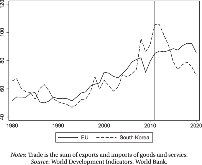
In order to illustrate how the EU and South Korea are integrated into the world economy, Fig. 1 displays their trade-to-GDP ratios for the year 1980-2020.Footnote 14 While these ratios moved in tandem more or less until 2007, South Korea’s ratio exceed that of the EU in 2008, reached its peak in 2011 (around 106%), but then fell to around 74% in 2016. The period of this drop coincides with the five years after the implementation of the EU-South Korea FTA. In the EU, the ratio increased only modestly, but steadily between 2008 (82%) and 2019 (92%), with a drop in 2009 due to the crisis. In the regression analysis below, the movements of the countries’ trade orientations will be captured by (role-specific country-and-time) fixed effects.
Table 1 lists the top trading partners of the EU and of South Korea for the years 2010 (one year before the agreement entered into force) and 2016 (five years after the agreement entered into force). In line with the regression analysis below, the numbers refer to trade in manufactured goods in current prices. With a volume of 34,841 billions USD, South Korea was the tenth largest destination for EU exports in 2010 (2.2% of total extra-EU exports) and the nineth largest export destination in 2016 (2.6%). South Korea was the sixth largest source country of EU imports in 2010 (4.2%) and the seventh largest source country in 2016 (3.6%). Thus, South Korea is in the group of the top ten trading partners of the EU, but only at the lower end when it comes to export destinations. Moreover, the share of imports from South Korea in total EU imports slightly declined between 2010 and 2016.
Taking now the perspective of South Korea, the EU was second largest export destination in 2010 (11.9%) behind China (25.9%) and the third largest in 2016 (9.9%) behind China (25.8%) and the US (13.9%).Footnote 15 The EU was the third largest source of imports in 2010 (14.1%) behind China (26.0%) and Japan (23.4%) and the second largest source of imports in 2016 (16.5%) behind China (32.3%). Thus, already before the agreement entered into force, the EU was a more important trading partner for the South Korea than vice versa.
The European Commission (2016) also documents that exports from the EU to South Korea increased in the years after the implementation of the agreement, while EU imports from South Korea declined in the first two years after the implementation and only returned to the level of the reference period in the forth year after the implementation (European Commission 2016, Graph 1). They argue that this decline is mainly driven by the fall in imports of Machinery & appliances, which – according to EC (2016) – account for 36% of EU imports from Korea, and decreased by 16%. EC (2016) concludes that “[t]he weaker performance of Korean exports of goods has to be seen in the context of the decreased demand in the EU following the financial crisis” (p. 12; see EC (2017) for a similar statement).
EU imports from South Korea still could rise relative to imports from other countries. Table 1, however, documents a decline in this share from 2010 to 2016. Moreover, Fig. 156 in Civic Consulting and Ifo Institute (2018) shows that the share of South Korea in total imports of the EU (labelled “exports to the EU” in the report) declines from 2007 until 2013, and only mildly rises thereafter.
In the regression analysis below, the financial crisis and country-specific characteristics will be captured by exporter-and-time and importer-and-time fixed effects. The analysis will also allow the trade effects to differ across directions of trade (exports vs. imports).
So far, the focus has been on the EU as a whole. Now turn to single EU member countries. For each EU member country, Table 2 displays the exports to and imports from South Korea in millions of USD and as a share in this country’s total extra-EU exports and total extra-EU imports, respectively. In terms of absolute volumes, the largest exporter to and the largest importer from South Korea in the EU is Germany, except for imports in 2016. For most of the EU member countries, exports to South Korea are larger in 2016 than in 2010. Exceptions are the Netherlands, Malta, Cyprus, and Bulgaria.
From 2010 to 2016, Germany’s imports from South Korea dropped by around 40%. Also many other countries see their imports from South Korea falling, although the percentage changes are typically smaller. But there also countries that see their imports from South Korea rising, namely the UK, Belgium-Luxembourg, Spain, Greece, the Czech Republic, Sweden, Cyprus, Slovenia, Romania, and Ireland.
Taking the observations on exports and imports by EU member country together, it can be expected that the effect of the EU South Korea FTA differs across EU member countries and for a given EU member countries across directions of trade (exports vs. imports).
I now turn to the relative importance of South Korea in EU countries’ extra-EU trade. The share of exports to South Korea in a country’s total extra-EU exports is highest for Cyprus (15.2% in 2010 and 12.9% in 2016, respectively), but typically the shares are below 3%. The share of imports from Korea in extra-EU imports of an EU member state was highest for Slovakia in 2010 (43.8%) and Cyprus in 2016 (28.8%). There are some countries which feature import shares higher than 10%. In 2016, also Slovakia, Slovenia, and Greece stand out in terms of the importance of South Korea in extra-EU imports.
A WTO report (WTO 2012) documents the commodity structure of merchandise trade between the EU and South Korea as well as with the world in the period 2008-2010. It turns out that machinery is very important for both trade in both directions. Looking first at exports from the EU to South Korea, machinery amounts to 29.1% of the EU’s global exports (largest commodity group), 25.6% of Korean global imports (second largest category behind minerals), and 40.2% of Korea’s imports from the EU. Turning now to imports of the EU from South Korea, machinery accounts for 34.6% of Korea’s global exports (largest category), 21.9% of the EU’s global imports (second largest category behind minerals), and 46.8% of the EU’s imports from Korea. Thus, aggregate EU imports from South Korea are dominated by trade in machinery.
The WTO (2012) also documents the liberalization schemes. Importantly, before the implementation of the agreement, 53.8% of EU imports from South Korea, but only 26.4% of Korea’s imports from the EU (average for 2008-2010 trade values) had been MFN duty free. Thus, exports and imports are asymmetrically affected, which again calls for exploring directional effects in the econometric analysis. By 2030, the EU will have liberalized all but 42 tariff lines related to agricultural products, and South Korea will have liberalized all but 57 tariff lines related to agricultural products and prepared foodstuffs. The EU eliminates duties faster than South Korea; see Lakatos and Nilsson (2017, Fig. 1). From this perspective, the effect on EU imports should be seen earlier than the effect on EU exports.
3 Structural Gravity Framework
In this section, I follow Yotov et al. (2016) in deriving the structural gravity system from the demand side for a single-sector endowment economy.
Basic Assumptions
Consider a world that consists of N countries, where each country i is endowed with \(Q_{it}\) units of a tradable variety of a differentiated good at time t. The factory-gate price for each variety is \(p_{it}\). The value of domestic production as well as nominal income in country i are given by \(Y_{it} = p_{it} Q_{it}\). Country i’s aggregate expenditure is denoted by \(E_{it}\).Footnote 16
Preferences
Simplify by assuming that each country is populated by a representative consumer whose preferences are represented by a Constant Elasticity of Substitution (CES) utility function
where \(c_{ijt}\) is the demand by consumers in country j for the good from country i at time t and \(\sigma >1\) is the elasticity of substitution between different varieties (goods from different countries). The parameter \(a_{it}\) represents the taste for good i at time t. The associated consumer price index is given by
where \(p_{ijt}\) is the price of good i in country j at time t.
Trade Costs
International trade between countries is subject to iceberg trade costs. In order to sell one unit of good i in country j, \(t_{ijt} \ge 1\) units have to be shipped, with \(t_{iit} = 1\). By the no-arbitrage condition, we must have \(p_{ijt} = t_{ijt} p_{it}\).
Bilateral Trade Flows
Maximizing consumer’s utility subject to the budget constraint, country j’s expenditure on good i emerges as
Market Clearance
Market clearance for good i at time t implies
The market clearing condition (4) can be solved for \(\left( \alpha _{it} p_{it}\right) ^{1-\sigma }\) as
Multiplying the numerator and the denominator by \(Y_t \equiv \sum _i Y_{it}\) and defining \(\Pi _{it}^{1-\sigma } \equiv \sum _j \left( \frac{a_{ijt} t_{ijt} }{P_{jt}} \right) ^{1-\sigma } E_{jt}/Y_t\), Eq. (5) can be rewritten as
Structural Gravity
Using Eq. (6) to substitute out \(\left( a_{it} p_{it}\right) ^{1-\sigma }\) from Eqs. (2) and (3) yields the structural gravity system
As in Yotov et al. (2016), the good-specific preference parameter \(a_{it}\) does not show up in the structural gravity system as its role is not distinguishable from the ex-factory price \(p_{it}\).
Trade Cost Function
Extending Baier et al. (2019) to potential anticipation effects, I assume the following specification of the trade cost term:
where \(Z_{ij}\) is a set of time-invariant controls for the general level of trade costs between i and j with coefficient vector \(\delta\) and \(RTA_{ijt}\) is a dummy variable that indicates whether the two trading partners i and j are both a member of the same RTA at time t. The RTA dummies capture the liberalization effects of both tariff and non-tariff barriers. More precisely, the coefficient \(\alpha\) captures the contemporaneous RTA effect, while the coefficients \(\alpha _{F,s}\) and \(\alpha _{L,k}\) capture the anticipation (Forward) and delayed (Lagged) effects by looking s years ahead and k years back, respectively.
While Eq. (10) only contains a single set of dummies for all RTAs, in the regressions below I will include an extra dummy for the EU-South Korea FTA and “purge” the set of RTA dummies from the EU-South Korea FTA. Thus, I can identify the effect of the average RTA other than the EU-South Korea FTA as well as the effect of the EU-South Korea FTA.
Empirical Gravity Equation
The empirical gravity equation becomes
where \(\eta _{it}\) is a set of exporter-and-time fixed effect absorbing all time-varying exporter-specific characteristics such as the outward multilateral resistance terms, \(\psi _{jt}\) is a set of importer-and-time fixed effect absorbing all time-varying importer-specific characteristics such as the inward multilateral resistance term, \(\gamma _{ij}\) is a (directional) pair fixed effect capturing \(Z_{ij}\) and absorbing all time-invariant country-pair specific characteristics, including those that could explain selection into an RTA, and \(\sum _t B_{ij,t}\) is a set of dummies equal 1 for international trade observations (as opposed to internal trade \(X_{ii}\)) at each time t, capturing the process of globalization over time, as all countries trade more with each other and less with their own internal markets (Bergstrand et al. 2015). The variable \(\varepsilon _{ij,t}\) is the error term.
Equation (11) can flexibly capture anticipation and delayed effects.Footnote 17 Using data from Baier et al. (2019) for 69 countries and the years 1986-2006, Egger et al. (2022) have empirically shown that the effect of the RTAs begins about three years prior to their entry into force and reach their full impact after ten years.
Variants of Eq. (11) will be estimated using a three-way FE-PPML estimator. PPML is recommended for use in gravity applications (Yotov et al. 2016). PPML typically outperforms linear (and other) specifications (Head and Mayer 2014; Egger and Staub 2016). An elegant feature is that PPML produces estimates in which, summing across all partners, actual and estimated total trade flows are identical (Arvis and Shepherd 2013; Fally 2015). I adjust for the (asymptotic) bias in the coefficient estimates as well as the standard errors applying the bias-correction methods developed by Weider and Zylkin (2021a).
Interpretation of Gravity Estimates
The estimated RTA coefficients can be used to compute the effects of the RTA on the volume of trade among member countries of the agreement in percentage terms according to \(\left( e^{\hat{\alpha }} - 1 \right) \times 100\).
The specification (11) allows to identify effects at different instances in time. It can also be used to compute the cumulative trade effect up to a certain point in time by first summing over the corresponding estimated RTA coefficients and then applying the above transformation.
It is important to note that all these effects are “partial” trade effects because they only capture the effect of bilateral trade cost changes on bilateral trade, holding time-varying characteristics of the exporting and the importing country (i.e. wages, multilateral resistance terms) and time-invariant characteristics of country pairs constant.
On top of trade volume effects, the estimated coefficients can be used to compute tariff equivalents of the RTA in percentage according to \(\left( e^{\hat{\alpha }/(-\sigma )} - 1 \right) \times 100\). In this formula, \(-\sigma\) is the elasticity of bilateral trade in tariffs.Footnote 18 Thus, in order to compute tariff equivalents, additional information on the elasticity of substitution is required.
4 Data
Data on international and intra-national trade in manufactured goods come from the WTO Structural Gravity Database (Monteiro 2020).Footnote 19 It covers the period 1980-2016 and includes 186 trading partners. Belgium and Luxembourg do not appear as separate countries, but are summarized as “Belgium-Luxembourg”.Footnote 20 For most of the countries, international trade flows are available for all years. Information for intra-national trade is not necessarily available for every year.Footnote 21
Information on RTAs comes from Mario Larch’s Regional Trade Agreements Database (Egger and Larch 2008, updated version). This dataset contains information on all multilateral and bilateral regional trade agreements as notified to the World Trade Organization for the years 1950 to 2019.Footnote 22 I update the RTA database to the years 2020 and 2021 using information from the WTO Regional Trade Agreements Database.Footnote 23 I create dummy variables for the EU-South Korea FTA and “purge” the RTA dummy from this FTA. Hence, the RTA dummy presents the average effect of all RTAs other than the EU-South Korea FTA, while the EU-South Korea dummy represents the effect of the EU-South Korea FTA.
In the final dataset, I can include up to 5-year lags and leads, respectively, of the EU-South Korea FTA dummy in the same regression (\(s^{\max }=5\), \(k^{\max }=5\)). The maximum number of the lag is determined by the difference between 2016 (the most recent year for which trade data are available) and the date of entry into force (2011 in the case of the EU-South Korea FTA).Footnote 24 Updating the RTAs to 2021 guarantees that the year 2016 is in the sample when a 5-year lead is included.Footnote 25
The bias-correction methods developed by Weidner and Zylkin (2021a, b) are very demanding in terms of memory requirements. For the regressions that explore heterogeneity in trade effects across pairs and across directions within pairs, Stata runs against the memory constraints of the computer and exits with an error when using the full dataset. Thus, for these regressions, I rely on a smaller dataset that comprises information on 76 countries. These 76 countries are the 69 countries that are in the dataset employed by Baier et al. (2019) plus 7 EU member countries that are not covered by their dataset.Footnote 26
5 Econometric Specifications and Results
In this section, I present the econometric specifications and the results. First, I explore how the EU-South Korea FTA affects total trade as well as exports and imports separately. Second, I explore heterogeneity across pairs and directions within pairs.
5.1 Average Effects of the EU-South Korea FTA
5.1.1 Allowing for Anticipation and Lagged Effects
In order to identify the trade effect of the EU-South Korea FTA, I augment Eq. (11) by adding a specific dummy for this agreement and purging the RTA dummy from this agreement. The estimation equation reads
The RTA dummy captures the effect of all RTAs other than the EU-South Korea FTA, while the dummy EUK captures the effect of the EU-South Korea FTA.Footnote 27
In the baseline specification, I account for four leads (\(s=4\)) and five lags (\(k=5\)) of the EU-South Korea FTA. For the other RTAs, I account for five leads and ten lags (see Egger et al. 2022). Column (1) of Table 3 displays the estimation results. Before turning to the effects of the EU-South Korea FTA, I dicuss the effects of RTAs other than the EU-South Korea FTA. The estimates of the leads are positive. All but the 2-year lead are also statistically significant. This finding is in line with Egger et al. (2022) who argue that “the impact of FTAs begins about 3 years prior to their entry into force” (p. 46). I find the contemporaneous effect of other RTAs not to be statistically significant, while Egger et al. (2022) report a statistically significant negative contemporanous effect. There is evidence for delayed effects. More precisely, the 1-year, the 4-year, the 5-year, and the 10-year lag are significantly positive, which is in line with the 10-year period postulated by Baier and Bergstrand (2007). In contrast to Egger et al. (2022), I find a relatively large and statistically significant positive 10-year lag. The estimated average total other RTA effect is 0.314, which is very close to the findings in Baier et al. (2019) and Egger et al. (2022). Thus, on average an RTA other than the EU-South Korea FTA has a partial effect of \(e^{0.314} - 1 \approx 37\%\) on bilateral trade flows. Setting \(\sigma =5\), other RTAs reduced bilateral trade costs by \(6.1\%\).
Now consider the effects of the EU-South Korea FTA. All but the 1-year lead are positive, and the 2-year lead is statistically significant. The 1-year lead, however, is statistically significantly negative. The contemporaneous effect of the EU-South Korea is positive, but not statistically significant. The 1-year lag is negative, but insignificant. All other lags are positive, and the 4-year lag is statistically significant. The cumulative effect of the EU-South Korea FTA five years after entry into force is 0.176 (with a standard error of 0.117). Ignoring the fact that the cumulative effect is imprecisely estimated, on average the EU-South Korea FTA increases trade between EU countries and South Korea by \(19.2\%\). With \(\sigma =5\), this amounts to a reduction of bilateral trade frictions by \(3.5\%\). The cumulative effect of the EU-South Korea FTA is smaller than that of other RTAs. This also holds if one only accounts for delayed effects until five years after the agreement, for which the cumulative effect is 0.253 (with a standard error of 0.064).
In column (2), I additionally include the 5-year lead of the EU-South Korea FTA. This 5-year lead should be insignificant, because the EU-South Korea FTA was only announced four years before it entered into force. Indeed, the 5-year lead is very small and insignificant.Footnote 28 All other coefficients remain virtually unaffected.
In a next step, I illustrate the effects of the EU-South Korea FTA and other RTAs in the course of time, as in Egger et al. (2022). To avoid blurring the cumulative trade effect by negative 5-year leads (for other RTAs), I re-estimate Eq. (11), restricting the number of leads to three. Column (3) of Table 3 displays the estimated coefficents. Reducing the number of leads affects the estimated coefficient for the 3-year lead, which seems to subsume the effects of earlier periods. The other coefficients and their standard errors as well as the cumulative effects are by and large unaffected. Figure 2 visualizes the cumulative trade effects and their 95% confidence intervals. For other RTAs, the pattern is similar to the one found by Egger et al. (2022). As I start from the 3-year lead, the effects in the period prior to the agreement are positive and statistically significant from the first year before the agreement. Moreover, I find a more pronounced jump in the first year after the agreement. Then there is a stready increase until the fifth year after the agreement. A further jump occurs in the tenth year after the agrement, while Egger et al. (2022) find a jump to occur in the seventh year after the agreement.
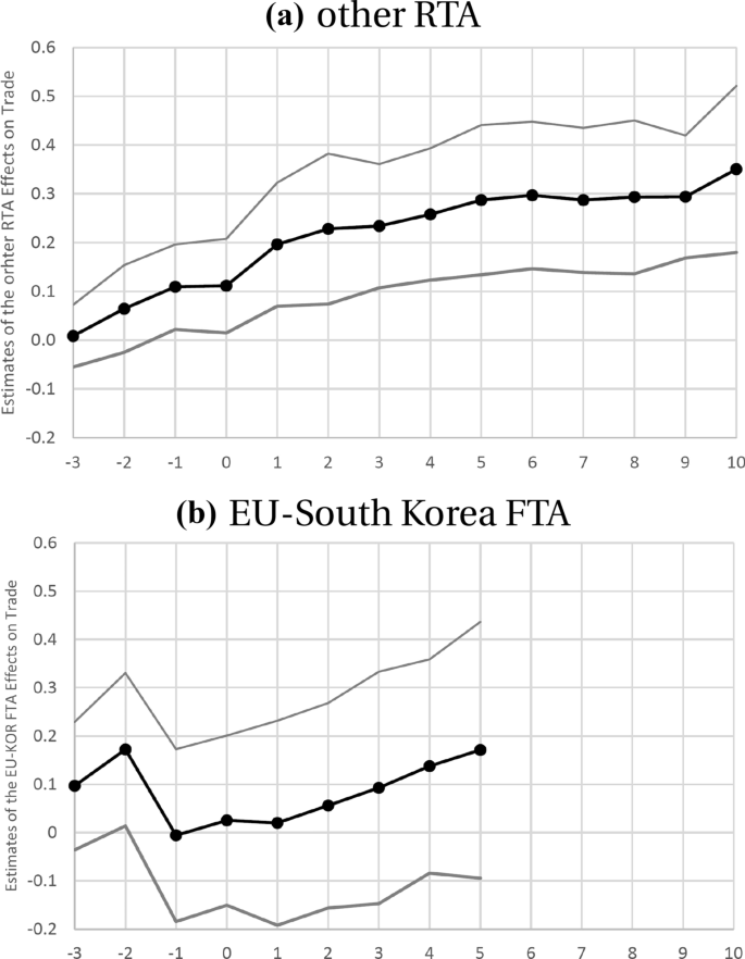
Cumulative effects of other RTAs and the EU-South Korea FTA
The EU-South Korea FTA effects show a different pattern. There are statistically significantly positive effects two year prior to the agreement, but these effects have vanished one year prior to the agreement. Starting from one year after the agreement entered into force, the effect steadily rises, but after a 5-year period, its magnitude is only comparable to the one other RTAs have reached after two years. Moreover, the effect is not statistically significant.
Finally, I present results from a regression where I use a somewhat coarser time structure. More precisely, I only consider the 3-year lead, the 5-year lag, and for other RTAs additionally the 10-year lag. Columns (4) and (5) of Table 3 show the result. In Column (4), I use the standard dataset. The 3-year leads are not statistically significant. The contemporaneous effect of other RTAs is large and highly significant, while the one of the EU-South Korea FTA is not. Both 5-year lags are positive and statistically significant. The cumulative effects obtained from this specification are comparable to the ones obtained from a specification with annual leads and lags, compare columns (2) and (3). In Column (5), I repeat the exercise on the smaller dataset that only contains 76 countries. This leaves the estimates of the trade effects of other RTAs by are large unchanged. The estimates of the trade effects of the EU-South Korea FTA are somewhat smaller.
5.1.2 Heterogeneity Across Directions of Trade
The estimates obtained in the previous subsection represent the effect of the EU-South Korea FTA on bilateral trade between EU member countries and South Korea. Almost any theory of specialization suggests the effects to be different for imports and export. I therefore now allow the effect to differ across directions of trade d, where d can be either exports or imports.Footnote 29 More specifically, I run the following regressions
Along with the contemporaneous effect, I consider the 3-year lead and the 5-year lag. For other RTAs, I additionally include the 10-year lag.
Table 4 displays the results. The effects of other RTAs are not affected by allowing for heterogeneity across directions of the EU-South Korea FTA, compare Table 4 to column (4) of Table 3. There are, however, differences in the effect of the EU-South Korea FTA across directions. The cumulative effect of the EU-South Korea FTA on exports of EU countries to South Korea is 0.329 (with a standard error of 0.155), which implies an increase in bilateral trade by \(39\%\).Footnote 30 This effect is smaller than the one reported by Civic Consulting and Ifo Institute (2018), who report a trade effect of \(54\%\) on exports of EU countries to South Korea. Recall, however, that while the present analysis takes two more years of adjustment into account, it is limited to manufactured goods. The cumulative effect of the EU-South Korea FTA that materializes after five years is slightly larger, however, than the effect that other RTAs reach after ten years, and substantially larger than the effect that other RTAs reach after five years.
Turning now to EU imports from South Korea, the 3-year lead and the 5-year lag are positive, but not statistically significant. The contemporanous effect, however, is large and negative, but also not significant. The cumulative effect on EU imports is positive, but not statistically significant.
These asymmetries in the effects on EU exports and imports might be related to the fact that South Korea is initially more reluctant on applying MNF duty free in EU imports and a less important destination for EU exports than vice versa. The fact that the EU is faster in liberalizing barriers on imports from South Korea than vice versa, however, does not materialize in an earlier effect on EU imports than on exports.
Asymmetries in the effects across directions have also been recognized by Civic Consulting and Ifo Institute (2018). They find a trade effect of 15% on EU imports from South Korea. Their analysis takes agriculatural goods, mining, and services into account, while the present analysis is limited to manufactured goods.
5.2 Pair-specific Effects
In the previous section, I have treated all EU countries in the agreement in the same way. However, they are still different countries. And “treatment” may mean different things in different times. Therefore, I now decompose the effect into two layers of heterogeneity. I start with presenting the effects for each country pair belonging to the agreement separately. Next, I consider the possibility that the effect of the EU-South Korea FTA differs across directions of trade within country pairs.
5.2.1 Heterogeneity Across Pairs
Let p denote country pairs that include an EU member country – either as an exporter or as an importer – and South Korea. The estimation equation to uncover pair-specific effects reads
For other RTAs, I take the contemporanous effect, lead 3, and lags 5 and 10 into account. For the EU-South Korea FTA, I account for contemporaneous effect, lead 3 and lag 5.Footnote 31 Thus, I estimate three coefficients for each of the 27 country pairs p in the EU-South Korea agreement (i.e., \(27 \times 3 = 81\) coefficients).Footnote 32
Table 5 displays the results of estimating Eq. (14). The first column presents the EU member country involved (the other country in the pair is always South Korea). Columns (1)-(3) report the lead, the contemporaneous, and the lagged effect, respectively. Column (4) displays the cumulative effect. The first and the second row represent, respectively, the point estimate and the standard error.
The following observations stand out. First, the cumulative effects are significantly positive for the Croatia, Czech Republic, Greece, Lithuania, Poland, Romania, Slovakia, and Slovenia, statistically negative for Bulgaria and Finland, and insignificant for the other 17 country pairs.Footnote 33 For most of these countries, the share of South Korea in extra-EU imports in the year 2010 are relatively high; see Table 2. Second, within the group of country pairs with significantly positive effects, cumulative effects range from 0.600 for Poland to 2.147 for Slovenia. Third, within the group of countries with significantly positive cumulative effects, there is heterogeneity in the timing of the effects. For Poland, the positive cumulative effect is entirely driven by anticipation effects, while for Croatia only the delayed effect is significant. Finally, almost all countries for which significantly positive cumulative effects arise have entered the EU in 2004 or later.Footnote 34 The integration of the new members may take time, which leaves room for differences in the starting conditions of the EU-South Korea FTA.
5.2.2 Heterogeneity Across Directions of Trade Within Pairs
I now allow the effects to differ across directions of trade within country pairs. Letting d denote the directions of trade, the estimation equation becomes
In this specification, I estimate three coefficients per direction d for each country pair p (i.e., \(27 \times 3 \times 2 = 162\) coefficients).
Table 6 displays the results of estimating Eq. (15) on the small sample with bias-corrected coefficients and standard errors.Footnote 35 The basic structure is the same as in Table 5, but instead of showing the effect on average trade per country pair, it displays the effects on exports of EU countries to South Korea in columns (1) to (4) and the effects on imports of EU countries from South Korea in columns (5) to (8).
The following observations stand out. First, out of the 54 cumulative directional effects, 18 show up significantly positive and 6 significantly negative.Footnote 36 Second, for Croatia, Cyprus, the Czech Republic, Lithuania, Poland, and Slovenia, both exports to and imports from South Korea are positively affected. However, the size of the effects differ across directions. It is larger on exports to than imports from South Korea for Cyprus and Romania, about equal for Poland, and larger on imports than on exports for the other countries. Moreover, for Hungary, Spain, and Romania only exports to South Korea, and for Greece, Malta, and Slovakia, only imports from South Korea are positively affected. Thus, there is substantial heterogeneity not only across countries, but also across directions within country pairs. Note again for most of these countries with positive effects, the share of South Korea in extra-EU imports in the year 2010 is relative high; see Table 2.
As for the pair-specific effects, almost all countries for which significantly positive cumulative effects arise in at least one direction of trade have entered the EU in 2004 or later, leaving room for differences in the starting conditions.Footnote 37 Moreover, even if the tariffs and non-tariff barriers might be the same for all EU member countries, the composition of bilateral trade differs across pairs and across imports and exports within pairs. This means that there is heterogeneity in trade-weighted tariffs, which implies differences in the ex ante trade barriers.
Based on Zylkin (2016), Larch et al. (2021) argue: “[i]f the [EU-Turkey Customs Union] has stronger effects in sectors and for country pairs that had a high liberalization potential (that is, a low initial openness), we expect a negative correlation between the estimated coefficients and estimated fixed effects.” (p. 257). Figure 3 is a scatterplot showing the shares of South Korea in, respectively, extra-EU exports and extra-EU imports in the year 2010 (initial bilateral openness) on the x-axis and the point estimates of the directional trade effects on the y-axis. Consider exports (blue crosses) and ignore Cyrpus for a moment. Then, a trendline would be downward-sloping. This would be in line with the idea that low initial openness is associated to large agreement effects. A trendline that includes Cyprus, however, would be upward-sloping. Turning to imports (red triangles), a trendline would be upward-sloping as well. This finding suggests that the trade effects are particularly large for pairs that have high levels of bilateral openness already in the initial situations and calls for a different explanation.Footnote 38

Share of South Korea in EU country’s extra-EU trade and heterogeneous effects of the EU-South Korea FTA
Second, country pairs may also differ in the range of products they trade with each other. Kehoe and Ruhl (2013) argue that country pairs trading a smaller range of product varieties before the trade negotiations start have a higher potential for trade growth thereafter. In the present paper, I do not explore their “least-traded goods hypothesis”.
Third, through the lens of the model, the estimated coefficients compound the semi-elasticity of trade costs in the RTA with the elasticity of bilateral trade in bilateral trade costs. In an Armington (1969) or a Krugman (1980) setting, the latter is governed by the elasticity of substitution between varieties.Footnote 39 These elasticities differ across products (Rauch 1999). Products featuring a low elasticity of substitution respond less to a given trade cost shock compared to products characterized by a large elasticity of substitution. Hence, when the product composition of trade flows differs across directions within pairs, the trade effects will differ as well.
6 Concluding Remarks
In this paper, I document substantial heterogeneity in the partial effects of the EU-South Korea FTA across time, country pairs, and directions within country pairs on bilateral trade in manufactured goods. In doing so, I contribute to the recent literature that stresses heterogeneity in the effects of trade policy changes. I find the phasing-in period of five years to be too short to find a significant average trade effect of the EU-South Korea FTA. Moreover, I fail to find a significant effect on EU imports of manufactured goods from South Korea. This implies that the positive effect on imports found by Civic Consulting and Ifo Institute (2018) must be driven by sectors other than manufacturing. Differences in the effects on EU exports and EU imports, however, are likely to reflect differences in ex ante trade barriers. Regarding country-specific estimates, I find significiant effects mainly for countries that have joined the EU relatively recently. Thus, the coefficients may reflect adjustments to EU membership or differences in the composition of trade with South Korea between new and old EU members. I find a positive correlation between directional trade effects and the inital share of South Korea in extra-EU-imports.
For a better understanding of the effect, it would be interesting to explore the margins through which the EU-South Korea FTA affects bilateral trade volumes. Using French customs data, Chowdhry and Felbermayr (2021) find that firms that are larger before the EU-South Korea FTA benefit more in terms of sales from the FTA than firms at the lower end of the size distribution.
Some of the estimated cumulative partial trade effects seem to be negative, which is not a new result. Baier et al. (2019) find a substantial share of agreement-by-pair and agreement-by-direction effects of the EU accession and other agreements to be negative; see their Table 2 and their Fig. 2.Footnote 40
The structural gravity system described in Sect. 3 can be derived under different sets of assumptions (Yotov et al. 2016). There are trade models, however, that do not predict a multiplicative form of the gravity equation.Footnote 41 Examples are gravity equations derived from linear demand systems (Ottaviano et al. 2002; Spearot 2013) or translog expenditure functions (Feenstra 2003; Novy 2013; and Chen and Novy 2021). Also in models with endogenous marketing costs, the effect of trade liberalization on small firms differs from the one on large firms, which makes the response of aggregate trade dependent on the composition of firms (Arkolakis 2010). Irarrazabal et al. (2015) explore the gravity equation – at the firm-level – in the presence of additive trade costs. Moreover, Adão et al. (2020) allow for a flexible parametrization of the productivity distribution in a monopolistic competition model with firm heterogeneity. There are also truely trade dynamic models (e.g., Alessandria et al. 2021). In all these models, trade elasticities are not constant. More importantly, they command a different specification of the gravity equation.
I leave a more sophisticated explanation for the heterogeneity of the trade effects and the use of other specifications of the gravity equation to future research. Moreover, it would be interesting to bring in other sectors like the service sectors again.
Notes
The World Trade Organization (WTO) classifies the following types of RTAs, defined under the General Agreement on Tariffs and Trade (GATT) and the General Agreement on Trade in Services (GATS): Customs Union (CU), Economic Integration Agreement (EIA), Free Trade Agreement (FTA), and Partial Scope Agreement (PSA). RTAs can be combinations of different types. In fact, the EU South-Korea FTA is classified as “FTA & EIA”.
In the regressions, they include country-and-time fixed effects rather than exporter-and-time and importer-and-time fixed effects. This is adequate only under the assumption of symmetric trade costs and the absence of trade deficits, because only then the outward and the inward multilateral resistance terms coincide, such that country-and-time effects suffice to control for both, outward and inward multilateral restistance.
The presence of domestic trade flows is also important to be able to identify trade diversion effects of RTAs (Dai et al. 2014).
As they include a 5-year lag, they can include RTAs that entered into force until 2001.
Baier et al. (2019) zoom into all RTAs in their dataset. Egger et al. (2022) use the same dataset as Baier et al. (2019), but mainly focus on the different phases that characterize the impact of the average RTA on bilateral trade and also explore the phases of the Canada-Chile Free Trade Agreement (CCFTA) and the Canada-Israel Free Trade Agreement (CIFTA), both launched in 1997.
Chowdhry and Felbermayr (2021) call this an ‘umbrella’ approach.
I use the command ppml_fe_bias proved by Weider and Zylkin (2021b). However, Stata runs against the memory constraints of the server and exits with an error in the pair-specific regressions. For these regressions, I use a smaller dataset; see below.
The dataset is also used by Larch et al. (2019b). There are alternative datasets that also feature intra-national trade. The dataset used by Baier et al. (2019) only covers the years 1986-2006 and therefore is not suited to study the trade effects of the EU-South Korea FTA. The second release of the World Input Output Database (WIOD, Timmer et al. 2015) covers the years 2000-2014, which only leaves room for a shorter phasing-in period. Moreover, Borchert et al. (2021) advise against using the WIOD data for estimation purposes because it “relies on economic models to estimate missing data” (p. 163). The International Trade and Production Database (Borchert et al. 2021) contains information at a more detailed industry level and additionally includes industries from agriculture, mining and energy, and services. However, as the dataset is unbalanced (some countries do not appear in some years and/or industries), one cannot aggregate up to these “broad sectors”. One could estimate industry-by-industry, but in the present context, this procedure would result in an unmanagable number of estimated coefficients. An alternative would be to pool across industries, but the biases that may arise in “four-way” gravity models have not been fully characterized yet (Weidner and Zylkin 2021a, p. 13).
Think of a machine that is ordered today but delivered only in the next year. This effect is conceptionally different from a dynamic adjustment that arises in models where foreign market entry costs are sunk (Das et al. 2007; Alessandria and Choi 2014) or the structure of export costs involves risk (Alessandria et al. 2021), which would command a dynamic specification of the gravity equation.
A new situation already arises with the beginning of the negotiations. As they continue, the uncertainty is gradually reduced.
For exports, the picture is less clear. Ignoring Cyprus, the correlation between the trade effect and the share of South Korea in the EU country’s extra-EU exports is negative, but with Cyprus, it is also positive.
In this figure, trade is the sum of exports and imports of goods and services.
The list of South Korea’s top 10 export destinations for manufactured goods in 2016 includes the Marshall Islands (1.6%). Note that also Malaysia (MYS) and Australia (AUS) reveive a share of 1.6% of exports from South Korea. Moreover, the export shares that go Philippines (PHL) and India (IDN) are 1.5% and 1.4%. In 2010, Malaysia received 1.1% of exports from South Korea.
Aggregate expenditure can also be expressed in terms of nominal income as \(E_{it} = \phi _{it} Y_{it}\), where \(\phi _i >1\) means that country i runs a trade deficit, while \(1> \phi _i >0\) reflects a trade surplus. Trade imbalanced are assumed to be exogenously given.
The number of leads s and lags k taken into account, however, is restricted to be the same for all RTAs.
Note that \(X_{ijt}\) denotes exports, which are computed exclusive of tariffs, which explains why tariff elasticity differs from the real trade cost elasticity, which is \(1-\sigma\).
The data do neither cover trade in agricultural products, fuels, and minining products nor in services.
The alpha-3 country ISO code of the conglomerate “Belgium-Luxembourg” is BLX.
For country and year coverage, see Monteiro (2020).
In the regressions, I include lagged information on RTA membership. For example, in regressions with a 10-year lag, bilateral trade in the year t (say, 1980), is related to the existence of an RTA in the year \(t-10\) (say, 1970).
For the year 2021, I only include RTAs that entered into force and appeared in the Database by July 7, 2021; see Table 8 in the Appendix for a list of RTAs that entered into force in 2020 and 2021. Most of the 42 agreements that entered into force in 2021 are agreements that involve the UK and substitute for agreements the UK formerly had under the umbrella of the EU, which has no effect on the coding of the RTA dummy.
Croatia joined the EU only in 2013 (and immediately entered the EU-South Korea FTA), so in regressions where I include country pairs separately, the number of lags for Crotia is restricted to 3.
In a regression with a 5-year RTA lead, bilateral trade in the year t (say, 2016) is related to the existence of an RTA in the year \(t+5\) (say, 2021).
The 7 additional countries are the Croatia (HRV), the Czech Republic (CZE), Estonia (EST), Latvia (LVA), Lithuania (LTU), Slovakia (SVK), and Slovenia (SVN).
For the sake of the focus on the EU-South Korea FTA, I ignore heterogeneity in the group of other RTAs.
Baier et al. (2019) who explore heterogeneous RTA effects warn that “[w]hile Baier and Bergstrand (2007) has emerged as the standard method for consistently estimating the average treatment effect of FTAs, the same cannot be said when we pull apart our average “\(\beta\)” to obtain increasingly more finely-grained coefficients, which we should regard as being estimated with at least some unobserved error” (p. 210). In the present analysis, I only zoom into a single RTA, as in Egger et al. (2022) and Larch et al. (2021).
With \(\sigma =5\), this implies a reduction in bilateral trade frictions by approx. \(6.4\%\).
As Croatia (HRV) joined the EU and hence the EU-South Korea Agreement only in 2013, I include lag 3 rather than lag 5.
Recall that Belgium and Luxembourg are merged to Belgium-Luxembourg in the trade data, such that in total there are 27 country pairs.
Baier et al. (2019) also find negative pair-specific EU accession effects for 24 country pairs.
The only exception is Greece. For Bulgaria, a significantly negative effect arises.
Table 9 in the Appendix display the results for the full sample, but without bias correction.
The significantly negative cumulative effects arise for Bulgaria (both trade directions), for exports of Malta, and imports of Denmark, Finland, and Ireland. Baier et al. (2019) report negative EU accession effects for some directed pairs. Larch et al. (2021) find negative effects on exports from Cyprus and Malta to Turkey
The exceptions are Finland and Greece.
In the Melitz (2003)-cum-Pareto model, this is the shape parameter of the Pareto distribution.
They also warn that the specific estimates are likely to “reflect omitted factors that may enter [the] specifications [...] via the error term” (p. 215).
Head and Mayer (2014) conclude that “the main reason to insist on the multiplicative form in the definition of gravity is historical usage. It is therefore possible that future work would abandon the multiplicative form and redefine gravity to allow other functional forms.” (p. 138).
References
Adão R, Arkolakis C, Ganapati S (2020) Aggregate Implications of Firm Heterogeneity: A Nonparametric Analysis of Monopolistic Competition Trade Models. NBER Working Paper No. 28081
Alessandria G, Choi H (2014) Establishment heterogeneity, exporter dynamics, and the effects of trade liberalization. J Int Econ 94(2):207–223
Alessandria G, Choi H, Ruhl K (2021) Trade adjustment dynamics and the welfare gains from trade. J Int Econ131, in print
Anderson JE, Larch M, Yotov YV (2017) Trade Liberalization, Growth, and FDI: A Structural Estimation Framework. Beiträge zur Jahrestagung des Vereins für Socialpolitik 2017
Anderson JE, van Wincoop E (2003) Gravity with gravitas. Am Econ Rev 93(1):170–192
Arkolakis C (2010) Market penetration costs and the new consumers margin in international trade. J Polit Econ 118(6):1151–1199
Armington PS (1969) A theory of demand for products distinguished by place of production. International Monetary Fund Staff Papers 16(1):159–178
Arvis JF, Shepherd B (2013) The poisson quasi-maximum likelihood estimator: A solution to the ‘Adding Up’ problem in gravity models. Appl Econ Lett 20(6):515–519
Baier SL, Bergstrand JH (2007) Do free trade agreements actually increase members’ international trade? J Int Econ 71(1):72–95
Baier SL, Yotov YV, Zylkin T (2019) On the widely differing effects of free trade agreements: Lessons from twenty years of trade integration. J Int Econ 116:206–226
Bergstrand JH, Larch M, Yotov YV (2015) Economic integration agreements, border effects, and distance elasticities in the gravity equation. Eur Econ Rev 78(C):307–327
Bhagwati J (1995) US Trade Policy: The Infatuation with Free Trade Agreements. In: Bhagwati Jagdish, Krueger Anne O (eds) The Dangerous Drift to Preferential Trade Agreements. AEI Press, Washington, DC
Borchert I, Larch M, Shikher S, Yotov Y (2021) The international trade and production database for estimation (ITPD-E). Int Econ 166(1):140–166
Breinlich H (2014) Heterogeneous firm-level responses to trade liberalization: A test using stock price reactions. J Int Econ 93(2):270–285
Chen N, Novy D (2021) Gravity and Heterogeneous Trade Cost Elasticities. CEPR Discussion Paper 16318
Chowdhry S, Felbermayr G (2021) Trade liberalization along the firm size distribution: The case of the EU-South Korea FTA. CESifoWorking Paper 8951
Civic Consulting and Ifo Institute (2018) Evaluation of the Implementation of the Free Trade Agreement between the EU and its Member States and the Republic of Korea. Directorate-General for Trade, European Commission
Correia S, Guimaraes P, Zylkin T (2019) ppmlhdfe: Fast Poisson Estimation with High-Dimensional Fixed Effects. arXiv:1903.01690
Correia S, Guimaraes P, Zylkin T (2020) Fast poisson estimation with high-dimensional fixed effects. Stata J 20(1):95–115
Dai M, Yotov YV, Zylkin T (2014) On the trade-diversion effects of free trade agreements. Econ Lett 122:321–325
Das S, Roberts MJ, Tybout JR (2007) Market entry costs, producer heterogeneity, and export dynamics. Econometrica 75(3):837–873
Egger P, Larch M (2008) Interdependent preferential trade agreement memberships: An empirical analysis. J Int Econ 76(2):384–399
Egger P, Larch M, Yotov YV (2022) Gravity-model estimation with time-interval data: Revisiting the impact of free trade agreements. Economica 89:44–61
Egger P, Staub KE (2016) GLM estimation of trade gravity models with fixed effects. Empir Econ 50(1):137–175
European Commission (2016) Annual Report on the Implementation of the EU-Korea Free Trade Agreement. Staff Working Document 162
European Commission (2017) Annual Report on the Implementation of the EU-Korea Free Trade Agreement. Staff Working Document 345
Fally T (2015) Structural gravity and fixed effects. J Int Econ 97(1):76–85
Feenstra RC (2003) A homothetic utility function for monopolistic competition models, without constant price elasticity. Econ Lett 78(1):79–86
Grübler J, Reiter O (2021) Non-tariff trade policy in the context of deep trade integration: An ex-post gravity model application to the EU-South Korea agreement. East Asian Economic Review 25(1):33–71
Handley K, Limão N (2015) Trade and investment under policy uncertainty: Theory and firm evidence. Am Econ J Econ Pol 7(4):189–222
Handley K, Limão N (2017) Policy uncertainty, trade, and welfare: Theory and evidence for China and the United States. Am Econ Rev 107(9):2731–2783
Head K, Mayer T (2014) Gravity Equations: Workhorse, Toolkit, and Cookbook.” In Handbook of International Economics, vol. 4, edited by Gita Gopinath, Elhanan Helpman, and Kenneth Rogoff, 131–95. Amsterdam: North-Holland
Irarrazabal A, Moxnes A, Opromolla L (2015) The tip of the iceberg: A Quantitative Framework for Estimating Trade Costs. Rev Econ Stat 97(4):777–792
Juust M, Vahter P, Varblane U (2020) Trade effects of the EU-South Korea free trade agreement in the automotive industry. Journal of East-West Business. https://doi.org/10.1080/10669868.2020.1732511
Kehoe TJ, Ruhl KJ (2013) How Important is the New Goods Margin in International Trade? J Polit Econ 121(2):358–392
Krugman P (1980) Scale economies, product differentiation, and the pattern of trade. Am Econ Rev 70(5):950–959
Lakatos C, Nilsson L (2017) The EU-Korea FTA: Anticipation, trade policy uncertainty and impact. Rev World Econ 153:179–198
Larch M, Monteiro JA, Piermartini R, Yotov YV (2019b) On the effects of GATT/WTO membership on trade: They are positive and large after all. WTO Staff Working Papers ERSD-2019–09
Larch M, Schmeisser AF, Wanner J (2021) A tale of (almost) 1001 coefficients: The deep and heterogeneous effects of the EU-Turkey Customs Union. J Common Mark Stud 59(2):242–260
Larch M, Wanner J, Yotov YV, Zylkin T (2019) Currency unions and trade: A PPML Re-assessment with High-dimensional Fixed Effects. Oxf Bull Econ Stat 81(3):487–510
Melitz MJ (2003) The impact of trade on intra-industry reallocations and aggregate industry productivity. Econometrica 71(6):1695–1725
Monteiro JA (2020) Structural Gravity Dataset of Manufacturing Sector: 1980–2016. World Trade Organization, Geneva
Moser C, Rose AK (2014) Who benefits from regional trade agreements? The view from the stock market. Eur Econ Rev 68:31–47
Novy D (2013) International trade without CES: Estimating translog gravity. J Int Econ 89(2):271–282
Ottaviano G, Tabuchi T, Thisse JF (2002) Agglomeration and trade revisited. Int Econ Rev 43(2):409–435
Rauch JE (1999) Networks versus markets in international trade. J Int Econ 48(1):7–35
Santos-Silva JMC, Tenreyro S (2006) The log of gravity. Rev Econ Stat 88(4):641–658
Spearot AC (2013) Variable demand elasticities and tariff liberalization. J Int Econ 89(1):26–41
Timmer MP, Dietzenbacher E, Los B, Stehrer R, de Vries GJ (2015) An illustrated user guide to the world input–output database: the case of global automotive production. Rev Int Econ 23:575–605
Weidner M, Zylkin T (2021a) Bias and consistency in three-way gravity models. J Int Econ 132
Weidner M, Zylkin T (2021b) Bias and consistency in three-way gravity models. arXiv preprint arXiv:1909.01327
World Trade Organization (2012) Free Trade Agreement between the European Union and the Republic of Korea (Goods and Services). WT/REG296/1/Rev.1
Yotov YV (2012) A simple solution to the distance puzzle in international trade. Econ Lett 117(3):794–798
Yotov YV, Piermartini R, Monteiro JA, Larch M (2016) An Advanced Guide to Trade Policy Analysis, The Structural Gravity Model. UNCTAD and WTO
Zylkin T (2016) Beyond Tariffs: Quantifying Heterogeneity in the Effects of Free Trade Agreements. GPN Working Paper Series 2016-006
Acknowledgements
I am grateful to Wilhelm Kohler and Julia Spornberger for thoughtful dicussions and comments. I am also grateful for comments from participants of the Hagen Workshop on Global Economic Studies in May 2021 and from two anonymous referees. I also thank Tom Zylkin for sharing the bias-correction command ppml_fe_bias_savev that saves the variance-covariance matrix. All remaining errors are mine.
Funding
Open Access funding enabled and organized by Projekt DEAL.
Author information
Authors and Affiliations
Corresponding author
Additional information
Publisher’s Note
Springer Nature remains neutral with regard to jurisdictional claims in published maps and institutional affiliations.
Appendix
Appendix
1.1 Additional Tables
See Table 7.
Rights and permissions
Open Access This article is licensed under a Creative Commons Attribution 4.0 International License, which permits use, sharing, adaptation, distribution and reproduction in any medium or format, as long as you give appropriate credit to the original author(s) and the source, provide a link to the Creative Commons licence, and indicate if changes were made. The images or other third party material in this article are included in the article's Creative Commons licence, unless indicated otherwise in a credit line to the material. If material is not included in the article's Creative Commons licence and your intended use is not permitted by statutory regulation or exceeds the permitted use, you will need to obtain permission directly from the copyright holder. To view a copy of this licence, visit http://creativecommons.org/licenses/by/4.0/.
About this article

Cite this article
Jung, B. The Trade Effects of the EU-South Korea Free Trade Agreement: Heterogeneity Across Time, Country Pairs, and Directions of Trade within Country Pairs. Open Econ Rev 34, 617–656 (2023). https://doi.org/10.1007/s11079-022-09690-6
Accepted:
Published:
Issue Date:
DOI: https://doi.org/10.1007/s11079-022-09690-6