Chaotic vibrations of flexible shallow axially symmetric shells

Abstract

In this work, chaotic dynamics of flexible spherical axially symmetric shallow shells subjected to sinusoidal transverse load is studied with emphasis put on the vibration modes. Chaos reliability is verified and validated by solving the implemented mathematical model by partial nonlinear equations governing the dynamics of flexible spherical shells and by estimating the signs of the largest Lyapunov exponents with the help of qualitatively different approaches. It is shown how the scenario of transition of the investigated shells from regular to chaotic vibrations depends on the boundary condition. The following cases are considered: (1) movable and fixed simple supports along the shell contours, taking into account shell stiffness (Feigenbaum scenario) and shell damping (Ruelle–Takens–Newhouse scenario), and (2) movable clamping (regular shell vibrations). The presence of dents, the location and character of which essentially depend on the shell geometric parameters, boundary conditions, and the external load parameters, is detected in some regions of the shell surface and discussed.

1 Introduction

Axially symmetric spherical shells, which are examples of thin-walled constructions, are widely applied in aviation and rocket industries, shipbuilding, automotive industries, energy-harvesting and chemical industries, fabrication of sensor devices, and bioengineering. In numerous constructions, the mentioned structural members are subjected to different external loads and boundary conditions, and thus, it is important to study their nonlinear vibrations.

The dynamics of flexible shells has a long history in mechanics, and only a selected part of it is considered in the present paper, putting emphasis on the novelty of the present work with respect to the findings in the available literature.

Baker [1] presented a theory predicting the existence of two infinite sets of the proposed normal shell model having bounded/unbounded frequencies for studying the axisymmetric modes of vibrations of thin spherical shells.

The transverse vibration of shallow spherical shells was investigated by Kalninis and Naghdi [2] and Kalninis [3, 4], including the shear theory and free vibration problems. Jain [5] analyzed the axisymmetric vibration of a shallow spherical shell subjected to time-varying loads, including the effects of transverse shear and rotary inertia. Special cases of the concentrated ring and central loads as well as the symmetrically distributed loads were also addressed.

The investigations devoted to studying the character of dents exhibited by shell surfaces were carried out by Volmir [6], Pogorelov [7], and Grigoluk and Kabanov [8], whereas the dents localization was analyzed by Mikhasev and Tovstin [9] with the help of the asymptotic methods.

Okazaki et al. [10] carried out a theoretical analysis of damping of the flexural vibration of a three-layer shallow spherical shell with a constrained viscoelastic layer. The influence of changes in the opening angle, shear parameter, layer thickness, and introduced boundary conditions on shell vibration was studied in terms of Bessel functions.

Evkin and Kalamkarov [11, 12] employed a perturbation analysis to large deflection of equilibrium states of composite shells of revolution. Evkin [13] proposed an asymptotic solution to the problem of large deflections of deep orthotropic spherical shells subjected to radial concentrated load.

Creep buckling of shallow arches was studied by Wang et al. [14].

Hamed et al. [15, 16] investigated creep buckling of imperfect thin-walled shallow concrete domes and nonlinear long-term behavior of spherical shallow shells of revolution.

Li et al. [17] analyzed the effect of spherical shell geometry and material properties on the critical normal load, interference, and the contact area where plastic yielding occurred. The authors proposed an empirically found relation for the load–interference spherical shell behavior prior to its plastic yielding.

Gurijala and Perati [18] studied axially symmetric vibrations of composite poroelastic spherical shell composed of two spherical shells. Biot’s theory was employed to derive the frequency equations for pervious/impervious shell surfaces. The dependence of nondimensional phase velocity on the ratio of outer and inner radii was estimated for two types of sandstone spherical shells.

Shi et al. [19] detected and studied the effects of curvature on the vibration characteristics of doubly curved shallow shells with general elastic edge constraints. A unified novel solution was proposed and validated by numerous tabular and graphical results illustrating the influence of curvature on the shell material frequencies for different boundary conditions.

However, no studies aimed at analyzing the modes of vibration of flexible circle axially symmetric shells subjected to uniformly disturbed harmonic loads have been found in the available, published literature. Furthermore, to the knowledge of the authors, the occurrence of localized dents exhibited by the spherical axially symmetric shells and their matching with the chaos theory is reported for the first time in the present manuscript.

Furthermore, novel scenarios of transition from regular to chaotic vibrations of the shell under the sinusoidal transverse load are presented for four boundary conditions (simple movable/nonmovable supports and movable/nonmovable clamping).

Our investigations are aimed at detecting “true” chaotic vibration. The vibration forms as well as the occurrence of located dents exhibited by flexible axially symmetric shallow shells depending on the employed boundary condition are studied.

The paper is organized in the following way: Sect. 2 deals with the problem statement, the mathematical model, and reduction from PDEs to ODEs by means of the FDM (finite difference method). Section 3 is devoted to studying the reliability and validity of the shell chaotic vibrations, whereas modes of nonlinear shell vibrations are investigated in Sects. 4 and 5.

Fig. 1

The studied axially symmetric shallow shell with the uniformly distributed harmonic load (a) and the scheme of a thin shell (b)

2 Problem statement and the method of solution

Let a spherical shallow shell be considered in the polar system of coordinates introduced in the following way: $\Omega = \left\{ { (r , z) } \right. \left| \right. r \in [0, b], \left. {{-h}/2 \le z \le h/2} \right\}$ (see Fig. 1a). Owing to the earlier work of Novozhilov [20], a shell is called thin if $h/R\ll 1$ (see Fig. 1b), and the inequality $h/R\le 1/40$ should be employed in such a case, as suggested by Novozhilov. If this inequality is not satisfied, then the shell is called thick. However, the majority of practically applied shells satisfy the inequalities $1/2000\le h/R\le 1/50,$ i.e., they belong to the class of thin shells. On the other hand, the threshold used to identify shallow shells is defined by the Reissner [21] ratio $f/2c<<1/8,$ where f is the distance between the shell vertex and a plane f and the distance 2c is measured in plane (see Fig. 1b). Vlasov [22] suggested $f/2c\le 1/5.$ Employing the Reissner criterion for shallowness $(\alpha <\alpha ^{*}=60^{\circ })$, one gets $2c\le R.$

The system of nonlinear PDEs governing dynamics of the axially symmetric shells has the following form [23]:

$$\begin{aligned}&\frac{\partial ^{2}w}{\partial t^{2}}+\varepsilon \frac{\partial w}{\partial t}=-\frac{\partial ^{4}w}{\partial r^{4}}-\frac{2}{r}\frac{\partial ^{3}w}{\partial r^{3}}+\frac{1}{r^{2}}\frac{\partial ^{2}w}{\partial r^{2}}- \nonumber \\&\qquad -\,\frac{1}{r^{3}}\frac{\partial w}{\partial r}-\frac{\varPhi }{r}\left( {1-\frac{\partial ^{2}w}{\partial r^{2}}} \right) -\frac{\partial \varPhi }{\partial r}\left( {1-\frac{1}{r}\frac{\partial w}{\partial r}} \right) \nonumber \\&\qquad +\,4q,\frac{\partial ^{2}\varPhi }{\partial r^{2}}+\frac{1}{r}\frac{\partial \varPhi }{\partial r}-\frac{1}{r^{2}}\frac{\partial \varPhi }{\partial r} \nonumber \\&\quad =\frac{\partial w}{\partial r}\left( {1-\frac{1}{2r}\frac{\partial w}{\partial r}} \right) ,\quad \varPhi =\frac{\partial F}{\partial r}. \end{aligned}$$

(2.1)

The below nondimensional quantities (with bars) are introduced:

$\bar{{t}}=\omega _0 t,\quad \omega _0 =\sqrt{{Eg}/{\gamma R^{2}}},\quad b=\left( {c/{\sqrt{Rh}}} \right) ,\quad \bar{{\varepsilon }}={\varepsilon R}/h\sqrt{g/{\left( {\gamma E} \right) }}, \quad \bar{{F}}={\eta F}/{Eh^{3}}, \quad \bar{{w}}={w\sqrt{\eta }}/h, \quad \bar{{r}}={br}/c, \quad \eta =12(1-\nu ^{2}), \quad \bar{{q}}=\bar{{q}}_3 =\left( {R/h} \right) ^{2}{q_3 \sqrt{\eta }}/{\left( {4E} \right) },$ where t[s]—time; $\varepsilon$[1/s]—coefficient of viscous-type external damping; F[Nm]—stress function; w[m]—deflection function; R[m], c[m]—main radius of the shell curvature and the radius of the shell contour, respectively; h[m]—shell thickness; b—shell parameter; $\nu$—Poisson’s coefficient; r[m]—distance between the rotation axis and the point of the shell middle surface; $q[\hbox {N}/\hbox {m}^{2}]$—amplitude of the external load; $\omega _0$[rad/s]—natural frequency of the small shell vibrations; $E[\hbox {N}/\hbox {m}^{2}]$—elasticity modulus; $g[\hbox {m}/\hbox {s}^{2}]$—gravity constant; and $\gamma [\hbox {N}/\hbox {m}^{3}]$—unit weight. (Henceforward, bars over the nondimensional quantities are omitted.) Dimensional PDEs can be found by means of substituting the above-mentioned nondimensional quantities to PDE (2.1) (see also [24, 25] and Appendix A). In the present investigations, we are aimed at studying the boundary conditions and two excitation parameters $q_0$ and $\omega _p$ of the sinusoidally distributed $q=q_0 \sin \omega _p t.$

The following boundary conditions are considered:

• (1) simple contour movable in the meridional direction

  

• (2) rigidly clamped contour

  

• (3) sliding clamping of the contour

  

• (4) simple nonmovable contour

  

Moreover, the following initial conditions $(^{\prime }=\frac{d}{dt})$

$$\begin{aligned} w = 0 , \quad {w}' = 0, \end{aligned}$$

(2.6)

as well as the below conditions in the vicinity of the shallow top are employed

$$\begin{aligned}&\varPhi _l \approx Ar, {\varPhi }'\approx A, w\approx B+Cr^{2}, {w}'\approx 2Cr, {w}'' \nonumber \\&\quad \approx 2C, {w}'''\approx 0. \end{aligned}$$

(2.7)

In order to reduce problem (2.1)–(2.7) governing dynamics of the considered continuous system to a system with lumped parameters, the finite difference method (FDM) with approximation $O (\Delta ^{2})$ is used. PDEs as well as boundary and initial conditions (2.1)-(2.7) are recast to the following finite difference formulas with respect to the spatial coordinate r and time:

$$\begin{aligned}&\ddot{w}^{i}+\varepsilon \dot{w}^{i}\nonumber \\&\quad =-\frac{w^{i+1} -w^{i-1} }{2\Delta }\left( {\frac{1}{r_i^3 }-\frac{\varPhi ^{i+1} -\varPhi ^{i-1} }{2r_i \Delta }} \right) + \nonumber \\&\qquad +\,\frac{w^{i+1} -2w^i +w^{i-1} }{r_i \Delta ^{2}}\left( {\varPhi ^i +\frac{1}{r_i }} \right) \nonumber \\&\qquad -\,\frac{\varPhi ^{i+1}-\varPhi ^{i-1} }{2\Delta }-\frac{\varPhi ^i }{r_i }-\nonumber \\&\qquad -\,\frac{w^{i+2}-4w^{i+1} +6w^i -4w^{i-1} +w^{i-2} }{\Delta ^{4}} \nonumber \\&\qquad -\,\frac{w^{i+2}-2w^{i+1} +2w^{i-1} -w^{i-2} }{2r_i \Delta ^{3}} \nonumber \\&\qquad +\,4q^i ,\varPhi ^{i+1} \left( {-\frac{1}{\Delta ^{2}}-\frac{1}{2r_i \Delta }} \right) +\,\varPhi ^i \left( {\frac{2}{\Delta ^{2}}+\frac{1}{r_i^2 }}\right) \nonumber \\&\qquad +\,\varPhi ^{i-1} \left( {-\frac{1}{\Delta ^{2}}+\frac{1}{2r_i\Delta }} \right) = \nonumber \\&\quad =-\frac{w^{i+1} -w^{i-1} }{2\Delta }\left( {1-\frac{w^{i+1} -w^{i-1} }{4r_i \Delta }} \right) , \end{aligned}$$

(2.8)

where $\Delta =b/n$ and n denotes the number of nodes of the shell radius.

The finite difference method (FDM) is employed only to spatial coordinates. It reduces the problem governed by PDEs (2.1) of an infinite dimension to the system of ODEs (2.8) with respect to time (the Cauchy problem). The Cauchy problem is solved using a few methods of the Runge–Kutta types, i.e., the fourth-order Runge–Kutta method (RK4), the second-order Runge–Kutta method (RK2), the fourth-order Runge–Kutta–Fehlberg method (RKF45), the fourth-order Cash–Karp method (RKCK), the eighth-order Runge–Kutta Prince–Dormand method (RK8pd), and the second-order and the fourth-order implicit Runge–Kutta method (rk2imp and rk4imp). After conducting numerous case studies, we have finally chosen the fourth-order Runge–Kutta method. The reason is that the accuracy of the this method is the same as of the Runge–Kutta methods of higher orders, but the computational time is shorter. Location of nodes along the shell radius r is shown in Fig. 2.

Fig. 2

Location of nodes

The counterpart difference forms of the boundary conditions are as follows:

• 1. Simple contour movable in the meridional direction

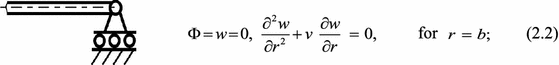
  $$\begin{aligned} \varPhi ^n= & {} 0,\quad w^{n+1} = \frac{\nu \Delta -2 b}{2 b + \nu \Delta } w^{n-1} ,\quad w^n \nonumber \\= & {} 0\hbox { for }r^n = b; \end{aligned}$$

  (2.9)

• 2. Rigidly clamped contour

  $$\begin{aligned} \varPhi ^{n+1}= & {} \varPhi ^{n-1} + \frac{2\Delta \nu }{b}\varPhi ^n ,\quad w^{n+1} \nonumber \\= & {} \frac{\nu \Delta -2 b}{2 b + \nu \Delta } w^{n-1} ,\quad w^n = 0\quad \hbox {for}\quad r^n = b;\nonumber \\ \end{aligned}$$

  (2.10)

• 3. Sliding clamping of the shell contour

  $$\begin{aligned} \varPhi ^n =0,\quad w^{n+1} = w^{n-1} ,\quad w^n = 0\quad \hbox {for}\quad r^n = b;\nonumber \\ \end{aligned}$$

  (2.11)

• 4. Simple nonmovable contour

  $$\begin{aligned} \varPhi ^{n+1}= & {} \varPhi ^{n-1} + \frac{2\Delta \nu }{b}\varPhi ^n ,\quad w^{n+1} \nonumber \\= & {} w^{n-1} ,\quad w^n = 0\quad \hbox {for}\quad r^n = b; \end{aligned}$$

  (2.12)

  and the below initial conditions are taken

  $$\begin{aligned} w^k = 0, {w}'^k = 0 , 0\le k\le m,\quad 0 \le t < \infty . \end{aligned}$$

  (2.13)

If small terms are neglected and differential operators are substituted by the central finite differences for $r=\Delta ,$ the following conditions are obtained at the top of the shell:

$$\begin{aligned} \varPhi ^0= & {} \varPhi ^2 -2\varPhi ^1 ; w^0 =\frac{4}{3}w^1 -\frac{1}{3}w^2; w^{-1} \nonumber \\= & {} \frac{8}{3}w^1 -\frac{8}{3}w^2 +w^3. \end{aligned}$$

(2.14)

The FDM (the finite difference method) is an alternative to the Faedo–Galerkin, the Ritz, and the finite element methods. Let us cite a few recently published papers, in which the FDM has been employed to study the dynamics of structural members.

Medina et al. [26] studied axially symmetric nonlinear behavior of electrostatically actuated and initially curved bistable microplates. Chen et al. [27] considered post-buckling of size-dependent microplate, focusing on damage effects due to the transverse load. Mehditabar et al. [28] carried out the thermoelastic study of a functionally graded piezoelectric rotating hollow cylindrical shell subjected to dynamic loads.

Aranda-Iglesias et al. [29] also investigated spherical shells. The solution was found using both the finite element method and the finite difference method. The same results were obtained for both methods, which validates the reliability of the FDM.

The transverse load can be changed arbitrarily with respect to the spatial coordinate and time. In this work, the harmonic transverse load of the form $q=q_0 \sin (\omega _p t),$ where $q_0$ stands for an amplitude and $\omega _p$ is a frequency of the excitation, is used.

3 Quantification of true chaotic vibrations

The problem related to reliability of chaotic vibration is extremely important, since in many cases errors introduced by numerical computations can be interpreted as chaotic behavior, which has been illustrated and discussed in reference [30]. It is known that one of the fundamental properties of chaotic dynamics is associated with its essential dependence on the initial conditions. On the other hand, more rigorous definition of chaos, given by Duavaney in 1989 [31], aside from the already mentioned property, emphasizes the importance of two other characteristics of chaos, i.e., intermittency/transitivity and regularity/periodicity conditions manifested by the density of periodic points. In 1992, Banks et al. [32] proved that the transitivity and periodicity conditions imply sensitivity to the initial conditions. On the other hand, Knudsen [33] defined chaos with the help of a function given on the bounded metric space, which is understood as a chaotic one if it exhibits a dense orbit and presents an essential dependence on the initial conditions.

Owing to Gulick results [34], chaos exists if sensitivity to the initial conditions is exhibited or a positive LE (Lyapunov exponent) is identified in each point of the space on which the chaotic function is defined, and the latter does not tend to periodicity. In this work, we employ the Gulick definition.

To solve the problem of reliability of chaotic vibrations while numerically solving nonlinear PDEs governing dynamics of spherical axially symmetric shells subjected to harmonic transverse load, the following steps are carried out:

• 1. Since PDEs are reduced to a Cauchy problem by means of the second-order FDM, the solution strongly depends on the number of nodes involved in the shell radius $r\in [0;b]$ partition. In the present paper, the solution is accepted if for n and $n + 1$ nodes the obtained solutions coincide. In particular, the convergence of the employed FDM is analyzed for different shallowness parameters and boundary conditions.

• 2. Since the Cauchy problem is also solved numerically, the solution essentially depends on both the used method and the employed time step. Therefore, the following methods are used: fourth- and second-order Runge–Kutta (RK4 and RK2) methods, the fourth-order Runge–Kutta–Fehlberg (RKF45) method, the fourth-order Cash–Karp (RKCK) method, the combination of the eighth-order Runge–Kutta and Dormand method (RK8pd), as well as the second- (rk2imp) and the fourth-order (rk4imp) implicit Runge-Kutta methods.

• 3. The numerically obtained data are used to construct the time series (signals), phase portraits, Fourier power spectra (FFT), Morlet wavelets, and shell deflection surfaces. The following wavelets are used: Meer wavelets, Shannon–Kotelnikov and Meier wavelets, Daubechies wavelets from db2 to db4, Coiflets, Morlet wavelets, complex Morlet wavelets as well as the wavelets based on the derivative of the Gauss function of order higher than 8. It should be emphasized that it was not feasible to investigate the considered problem with Meer and Shannon–Kotelnikov wavelets, i.e., the first one did not identify the frequency zones properly, whereas the second one did not yield the expected localization in time. The carried out analysis of the wavelet spectra obtained by the Daubechies wavelets, Coiflets, and simlets has shown that an increase in the order of the employed filter improves proper frequency identification. Furthermore, in spite of the differences between the employed wavelets and their filters, the wavelet spectra yielded by the Daubechies wavelets, simlets, and Coiflets of the same order give almost the same results. However, the frequency localization yielded by them is not accurate enough, which makes them unsuitable for analysis of vibration of the investigated mechanical system.

  Considering the results obtained by means of derivatives of the Gauss functions, the accuracy of the frequency localizations increased with the increase in the order of the derivative. It should be noted that the frequency spectra obtained by the Meer wavelet, which is a smooth variant of the Shannon–Kotelnikov wavelet, have been localized better than in the case of Morlet wavelets only for a low-frequency band. In what follows we give results for Morlet wavelets that were specially chosen and adopted to study the stated problem. In these wavelets, there is no scale function $\varphi$, and $\psi$ is given explicitly, i.e., there is no compact carrier. Therefore, to study complex vibration of continuous mechanical system, like a plate/shell, one can employ either complex or real Morlet wavelets or wavelets based on either real or complex derivatives of the Gauss functions of the order higher than 16.

• 4. Since the definition of chaos given by Gulick [34] is used in this work, one needs to compute Lyapunov exponents (LEs) and define their signs. In this paper, a spectrum of the LEs for each partition of the interval [0; b] was obtained by three methods: Wolf’s [35], Rosenstein’s [36], and Kantz’s [37]. Furthermore, convergence of the above-mentioned methods was also investigated.

The final solution was accepted and treated as reliable/true if coincidence up to four digits after the decimal point was achieved. According to the already given steps of investigation, convergence of the solution depending on the number n of partitions of the shell radius was considered at first. The study was carried out for all types of boundary conditions: movable simple support (2.9), rigid clamping (2.10), movable clamping (2.11), and nonmovable simple support (2.12) for $b\in [3;8].$ Then, results for $n = 10,\, 20,\, 40,\, 80, \,100, \,120,\, 140$ were compared.

After reducing problem (2.1)–(2.5) to its counterpart normal form, the first equation of the Cauchy problem was solved by the Runge–Kutta methods with respect to the deflection function w. At the same time, algebraic equations were solved (on each time step) with respect to the stress function O(r, t) by the method of inverse function. The time step was yielded by the Runge principle. The computational results in the form of frequency power spectra, wavelet spectra, and the surfaces of shell deflection for fixed time instances $t = 300$, $t = 304$, and $t = 305$ are reported in Table 3. The power spectrum obtained for $n = 10$ yields chaos spanned on five frequencies. In addition, the associated wavelet spectrum exhibits intermittency for $n = 10$, whereas for $n = 20$, chaos spanned on $\omega _p$ occurs (For $n=40$, one can detect $\omega _p , \, \omega _p /2, \, \omega _p /4$, and $3\omega _p /4$.) Since the latter behavior is exhibited by both FFT and wavelet spectrum, where intermittency does not appear, the number of partitions of the radius plays a crucial role in identifying the scenario of transition from periodic to chaotic vibrations.

Fig. 3

Convergence of FDM regarding time history w(t) versus the number of partitions of the radius n (a) and the window “a” for $t\in [290;330]$ (b)

Furthermore, convergence of the deflection surfaces was investigated at the same time instances. As the reported graphs show, the surfaces coincide only for $n = 120$ and $n = 140$. To make the results more clear, each of the 3D surfaces is supplemented with the deflection isoclines. Figure 3a presents the time histories/signals in relation to the number n of partitions of the shell radius. (Figure 3b reports a window of the signal in the interval $t\in [290;330]$.) Remarkably, for $n = 120$ and $n = 140$, the graphs coincide.

Integration with respect to time was also carried out by both explicit and implicit Runge–Kutta methods of different orders, as it is shown in Table 1. It is worth mentioning that triangular or arbitrary matrices are used in explicit and implicit methods, respectively.

Table 1 Methods used in numerical simulations

Table 2 Frequency power spectra for different n and different $q_{0}$

The methods RKF45, RKCK, and RK8pd allow for an automatic change of the integration steps as well as control of the integration errors. The carried out investigations showed that the fourth-order Runge–Kutta method is optimal to investigate the chaotic vibration of the considered flexible spherical shell subjected to harmonic load.

To discuss how the scenario to chaos will be changed while the number of nodes increases in the FDM, let us begin with the results reported in Table 2.

Table 3 Number of radius partitions n, power spectra, 2D wavelet spectra, and the shell deflection surfaces at three different time instants

In this table the frequency power spectra are reported for the vibration signals obtained with the FDM for different node numbers $n=20; \,40; \,80; \,120$. For $q_{0}=0.9$, all frequency spectra exhibit $\omega _{p}$ and $\omega _{p}/2$. Amplitudes of these harmonics are the same for all employed n. For $q_{0}=0.1335$, the regular bifurcations are exhibited on the frequencies $\omega _{p}$, $\omega _{p}/2$, and $\omega _{p}/4$ also for all $n=20; \,40; \,80; \,120$ nodes, but the values of harmonic amplitudes associated with $\omega _{p}/4$ are different for different n. This requires the use of higher number of nodes, i.e., the convergence of the results is achieved for $n=80; \,120; \,140; \,160$. In the case of $q_{0}=0.1395$, the vibration signals and their frequency characteristics strongly differ from each other: For $n=20$, we have chaos with the distinguished $\omega _{p}$ and $\omega _{p}/2$; for $n=40$, we have also chaos, but with dominating $\omega _{p}$ and $\omega _{p}/4$, whereas for $n=120; \,140; \,160$, one deals with quasi-periodic vibration associated with the frequencies $\omega _{p}$, $\omega _{p}/2$, $\omega _{p}/4$, $\omega _{p}/8$, and $\omega _{p}/16$. For $q_{0}=0.14$, beginning already from $n=20$, the obtained results coincide, exhibiting the system chaotic vibrations. Thus, the following conclusion can be yielded. A number of nodes employed in the FDM should be chosen differently for different vibrational regimes. Namely, periodic regimes require $n=20$ nodes, whereas quasi-periodic/chaotic regimes require $n=80$ or $n=120$. It means that if one investigates a mechanical system with an infinite number of degrees of freedom, one has to investigate the convergence of numerical solutions obtained by the finite difference method in order to get reliable/true results.

Fig. 4

Shell cross sections for different n at three time instants

Table 3 contains frequency power spectra (FFT), 2D wavelet spectra, and deflection forms of the shell surfaces at three different time instants, put one next to another for better clarity of the obtained results. Figure 4 reports the shell cross sections obtained for different n at three chosen time instants. The LEs computed by Wolf’s, Rosenstein’s, and Kantz’s methods are given in Table 4. It should be emphasized that to get reliable chaotic dynamics, a few different methods should be employed to compute LEs. In the present work, $n = 100; \,120; \,140$ were used in the FDM, and the obtained LEs coincide to three decimal places for all three considered methods. In the case of LEs computed for $n = 140$ by both Rosenstein’s and Kantz’s methods, the results coincide up to three decimal places, whereas in the case of Wolf’s method, the values of LEs are three times larger than those yielded by the remaining methods. Finally, $n = 120$ was used in further computations.

The carried out preliminary investigations allow one to perform reliable analysis of mechanical systems with infinitely many degrees of freedom.

Table 4 Calculated values of the LEs versus the number n of partitions of the shell radius

4 Modes of vibrations (simple support)

In 1978, Feigenbaum [38] proposed a universal mechanism of period-doubling bifurcation route to chaos. The Feigenbaum scenario was validated for the simply supported (2.2) axially symmetric spherical shells subjected to transverse harmonic load in reference [39], where the following parameters were used: $b=4, \quad \varepsilon =0.01$ (damping coefficient), $\nu =0.3$ (Poisson’s ratio), $t\in [0,1400]$, $\omega _p =\omega _0 =0.516$, and $q_0 \in [0.01,0.15]$ (amplitude of harmonic excitation). As the excitation frequency $\omega _p$ was equal to the shell frequency $\omega _0$, the case of the fundamental resonance was considered.

Six Hopf bifurcations were detected and served later for estimation of the Feigenbaum constant yielding $\alpha _6 = 4.65608466$. (The exact numerical value obtained by Feigenbaum equals 4.66916224 and differs by 0.28% from the above-mentioned numerical results.)

The signals obtained in the present numerical experiments have the amplitude–time representation. However, in order to understand the behavior of any dynamic system under action of an arbitrary external load, and to control the system, one needs to have an insight into information hidden in the frequency space of the signal. For this reason, the wavelet transform approach was employed. Recall that the wavelet-based analysis enables one to detect and trace the localized particular features of the signal, whereas the Fourier-based approach (FFT) makes it possible to follow the signal properties on the whole investigated time interval (see the description given in Sect. 3).

Table 5 Fourier frequency power spectra, 2D wavelet spectra, $(w,\dot{w},\ddot{w})$ phase plots, time history with marked time instants a, b, c, shell surface cross sections, and shell 3D shapes at a, b, c for different values of $q_{0}$ (simple support)

An increase in the number of new frequencies in the spectrum of vibration of the system yields a decrease in the informative properties of the employed wavelets, since harmonics with larger power shadow those with less power. Aside from this, it should be noted that the wavelet spectrum significantly depends also on the employed wavelet. (Each wavelet exhibits its own properties and peculiarities.) Therefore, to obtain reliable results, it is recommended to use both FFT and wavelet spectra simultaneously. The so far presented remarks concerning investigation of continuous structural systems were taken into account while constructing Table 5, where the Fourier frequency power spectra, 2D wavelet spectra, $(w,\dot{w},\ddot{w})$ phase plots, time history with marked time instants a, b, c, and the snapshots of the shell surface cross sections and the shell 3D shapes at a, b, c are reported for different values of $q_{0}$. (A similar table was constructed when studying the problem with boundary conditions (2.3).)

In the considered case, six period-doubling bifurcations were numerically detected and the Feigenbaum constant was estimated. The investigations showed that for the implemented boundary condition, a transition from periodic to chaotic vibrations is carried out following the Feigenbaum scenario. Remarkably, owing to the employed boundary conditions, one of the ribs at the surface of the shell deflections occurred regardless of the amplitude of the excitation load, i.e., the occurrence of the mentioned rib was not influenced by the number of the Hopf bifurcations. Furthermore, the mentioned rib appeared at the time instants when the shell top deflection was close to zero.

5 Modes of vibrations (rigid clamping)

In this section, vibrations of rigidly supported spherical shell ($b = 8$; boundary conditions (2.3)) subjected to the harmonic load $q_0 =\left\{ {0.01; 0.17; 0.21} \right\}$ and $\omega _p = 1.34$ close to $\omega _0$ are studied. Namely, the case of the fundamental resonance is investigated. The associated dynamic characteristics, similar to those reported in Table 5, are shown in Table 6. In this case, a transition from regular to chaotic vibrations follows the Ruelle–Takens–Newhouse route, i.e., the increase in the excitation amplitudes yields the birth of the independent frequency, which is linearly dependent on the excitation frequency. For $q_0 =0.01$, the shell exhibits a periodic regime. (Phase portraits present ellipses, whereas the LLE is less than zero.) The shell surface deflections exhibit two ribs, which occur at time instants when the shell center deflection is close to zero. An increase in the excitation load amplitude up to $q_0 =0.17$ yields the occurrence of an independent frequency. Furthermore, the ribs are exhibited by the shell surface, and the LLE>0. The wavelet spectrum and the FFT spectrum also report the independent frequency, and a linear combination of the excitation and independent frequencies is observed. The investigations imply that in the case of the rigidly clamped axially symmetric spherical shell, a transition from regular to chaotic vibrations is realized via the Ruelle–Takens–Newhouse scenario along the shell contour. Moreover, deflection of the shell surfaces exhibits from one up to four ribs. It is worth mentioning that the Ruelle–Takens–Newhouse scenario plays a crucial role in the ribs occurrence. Namely, the presence of only one rib is associated with regular shell vibration, two ribs are associated with the occurrence of the independent frequency, whereas the occurrence of chaos yields the existence of up to three ribs.

Table 6 Fourier frequency power spectra, 2D wavelet spectra, $(w,\dot{w},\ddot{w})$ phase plots, time history with marked time instants a, b, c, shell surface cross sections, and the shell 3D shapes at a, b, c for different values of $q_{0}$ (rigid clamping)

6 Investigation of occurrence of ribs (simple nonmovable shell support)

This section is devoted to vibrations of the axially symmetric shell with simple nonmovable support of its contours and the shallow parameter $b = 4$. If the shell is subjected to transverse and uniformly disturbed harmonic load, a period-doubling route to chaos following the Feigenbaum scenario is detected and seven Hopf bifurcations can be estimated numerically. Contrary to the previous examples, the number of the detected ribs is not fixed, but changes in time (Table 7). Changes in the vibration character do not influence the number of the detected ribs, i.e., the Feigenbaum scenario does not influence the number of ribs.

7 Shell vibration modes (movable clamping)

In what follows, vibrations of a spherical axially symmetric shell are considered for fixed parameters $b=5,\quad \varepsilon =0.1$. The presence of the Sharkovskii’s orbits is detected for the transverse uniform harmonic load $q=q_0 sin\omega _0 t$ for the case of movable clamping (2.4) and for zero initial conditions (2.6). The shell is made from an elastic, homogenous, and isotropic material with $\nu = 0.3$, and it is excited by the frequency $\omega _p$ being equal to the fundamental shell frequency $\omega _0 =0.773$ (linear vibration). Phase portraits (3D), frequency power spectra, wavelet-based analysis results, and the shapes of the shell surface deflections are reported. Table 8 shows the Sharkovskii’s ordering 3, $3^{2}$. The detected Sharkovskii’s ordering occurred successively, and this novel result, to the knowledge of the authors, is reported for the first time in the literature. It should be mentioned that Sharkovskii’s windows have been already detected and illustrated when studying vibration of beams.

For the applied boundary conditions, one time-dependent rib was detected in the snapshots of the shell main cross sections. Here, no relationship between the vibration regimes and the number of ribs was found.

Table 7 Fourier frequency power spectra, 2D wavelet spectra, $(w,\dot{w},\ddot{w})$ phase plots, time history with marked time instants a, b, c, and the snapshots of the shell surface cross sections and the shell 3D shapes at a, b, c for different values of $q_{0}$ (simple nonmovable shell support)

Table 8 Fourier frequency power spectra, 2D wavelet spectra, $(w,\dot{w},\ddot{w})$ phase plots, time history with marked time instants a, b, c, and the snapshots of the shell surface cross sections and the shell 3D shapes at a, b, c for different values of $q_{0}$ (movable clamping)

8 Concluding remarks

In the present paper, novel results of the study of chaotic vibration of flexible circular axially symmetric shallow shells subjected to sinusoidal transverse load were presented for four different boundary conditions . The study was conducted with the use of the finite difference method (FDM), which differentiates the study from the majority of research conducted with the finite element method (FEM).

The rigorous discussion of the advantages of the FDM can be found in numerous papers, including [40, 41]. The shells considered in the present study are axially symmetric, and hence, they are simpler for investigation in comparison with, for instance, geometric nonlinear shallow rectangular shells of the second-order accuracy.

It should be emphasized that in the paper [42], the authors studied the dynamics of geometrically nonlinear beams by means of employing both the FEM in the Galerkin form and the FDM. The solutions obtained with the use of these methods coincided, but the FDM allowed one to obtain the solution 1.5 times faster than the FEM.

Finally, there are numerous products aimed at solving the application-oriented problems of the theory of elasticity, such as ANSYS, ABACUS, COMSOL, where FEM is used. One of the serious drawbacks of the mentioned commercial products is that they employ the dimensional equations and the computational time is very long.

The conducted investigations allow one to formulate the following general conclusions.

• 1. A general methodology for detection and analysis of reliable/true chaos in the case on nonlinear vibration of flexible and axially symmetric shells subjected to uniformly disturbed harmonic load was proposed.

• 2. It was detected, illustrated, and discussed that the employed boundary conditions significantly influence the obtained solutions. For simple nonmovable and movable supports of the shell, for $\omega _p =\omega _0 ,$ a transition from regular to chaotic shell vibration was realized following the Feigenbaum scenario, whereas for a rigidly clamped shell, a transition to chaos followed the Ruelle–Takens–Newhouse scenario. Finally, in the case of the movable clamped shell, a series of Sharkovskii’s windows was reported.

• 3. It was found that the number of ribs exhibited by the shell surface strongly depends on the boundary conditions. The maximum number of ribs was detected for the shell with movable simple support, one rib was found for the shell with nonmovable simple support and the shell with movable clamping, whereas three ribs were detected in the case of rigid clamping.

Appendix A

The transition from dimensional to nondimensional PDEs is based on the theory of similarity and dimensional analysis. A general description of the methodology can be found in the books [24, 25].

Using the approach described in the above-mentioned references, one can find the following nondimensional quantities:

$$\begin{aligned} \bar{{t}}= & {} \omega _0 t,\quad \omega _0 =\sqrt{{Eg}/{\gamma R^{2}}},\quad b \nonumber \\= & {} \left( {c/{\sqrt{Rh}}} \right) ,\quad \bar{{\varepsilon }}={\varepsilon R}/h\sqrt{g/{\left( {\gamma E} \right) }}, \nonumber \\ \bar{{F}}= & {} {\eta F}/{Eh^{3}},\quad \bar{{w}}={w\sqrt{\eta }}/h,\quad \bar{y} \nonumber \\= & {} {by}/c,\quad \eta =12(1-\mu ^{2}), \nonumber \\ \bar{{q}}= & {} \bar{{q}}_3 =\left( {R/h} \right) ^{2}{q_3 \sqrt{\eta }}/{\left( {4E} \right) },\quad \bar{{x}}={bx}/c. \end{aligned}$$

(A1)

Relations (A1) yield the dimensional relations expressed by the nondimensional ones, and after substituting them to the following dimensional equations

$$\begin{aligned} \frac{Eh^{3}}{\eta }\nabla ^{4}w= & {} \frac{1}{R}\nabla ^{2}F+L(F,w) \nonumber \\&+\,q-\frac{\gamma h}{g}\frac{\partial ^{2}w}{\partial t^{2}}-\varepsilon \frac{\partial w}{\partial t}, \nonumber \\ \frac{1}{Eh}\nabla ^{4}F= & {} -\frac{1}{R}\nabla ^{2}w-\frac{1}{2}L(w,w), \end{aligned}$$

(A2)

one obtains

$$\begin{aligned}&\frac{Eh^{3}}{\eta }\left( \frac{\partial ^{4}\left( {\bar{{w}}h/\sqrt{\eta }} \right) }{\partial \left( {\frac{\bar{{x}}c}{b}} \right) ^{4}}+2\frac{\partial ^{4}\left( {\bar{{w}}h/\sqrt{\eta }} \right) }{\partial \left( {\frac{\bar{{x}}c}{b}} \right) ^{2}\partial \left( {\frac{\bar{{y}}c}{b}} \right) ^{2}} +\frac{\partial ^{4}\left( {\bar{{w}}h/\sqrt{\eta }} \right) }{\partial \left( {\frac{\bar{{y}}c}{b}} \right) ^{4}} \right) \nonumber \\&\quad =\frac{1}{R}\left( \frac{\partial ^{2}\left( {\frac{\bar{{F}}Eh^{3}}{\nu }} \right) }{\partial \left( {\frac{\bar{{x}}c}{b}} \right) ^{2}} +\frac{\partial ^{2}\left( {\frac{\bar{{F}}Eh^{3}}{\nu }} \right) }{\partial \left( {\frac{\bar{{y}}c}{b}} \right) ^{2}} \right) \nonumber \\&\qquad +\,\frac{\partial ^{2}\left( {\bar{{w}}h/\sqrt{\eta }} \right) }{\partial \left( {\frac{\bar{{x}}c}{b}} \right) ^{2}}\frac{\partial ^{2}\left( {\frac{\bar{{F}}Eh^{3}}{\nu }} \right) }{\partial \left( {\frac{\bar{{y}}c}{b}} \right) ^{2}} +\frac{\partial ^{2}\left( {\frac{\bar{{w}}Eh^{3}}{\nu }} \right) }{\partial \left( {\frac{\bar{{y}}c}{b}} \right) ^{2}}\frac{\partial ^{2}\left( {\frac{\bar{{F}}Eh^{3}}{\nu }} \right) }{\partial \left( {\frac{\bar{{x}}c}{b}} \right) ^{2}} \nonumber \\&\qquad -\,2\frac{\partial ^{2}\left( {\bar{{w}}h/\sqrt{\eta }} \right) }{\partial \left( {\frac{\bar{{x}}c}{b}} \right) \partial \left( {\frac{\bar{{y}}c}{b}} \right) }\frac{\partial ^{2}\left( {\bar{{F}}h/\sqrt{\eta }} \right) }{\partial \left( {\frac{\bar{{x}}c}{b}} \right) \partial \left( {\frac{\bar{{y}}c}{b}} \right) }+ \nonumber \\&\qquad +\,\bar{{q}}\frac{4Eh^{2}}{R^{2}\sqrt{\nu }}-\frac{\gamma h}{g}\frac{\partial ^{2}\left( {\bar{{w}}h/\sqrt{\eta }} \right) }{\partial \left( {\bar{{t}}\sqrt{\frac{\gamma R^{2}}{Eg}}} \right) ^{2}} \nonumber \\&\qquad -\,\bar{{\varepsilon }}\sqrt{\frac{\gamma E}{g}}\frac{h}{R}\frac{\partial \left( {\bar{{w}}h/\sqrt{\eta }} \right) }{\partial \left( {\bar{{t}}\sqrt{\frac{\gamma R^{2}}{Eg}}} \right) }, \frac{\partial ^{4}\left( {\bar{{F}}h^{3}/\nu } \right) }{\partial \left( {\frac{\bar{{x}}c}{b}} \right) ^{4}}\nonumber \\&\qquad +\,2\frac{\partial ^{4}\left( {\bar{{F}}h^{3}/\nu } \right) }{\partial \left( {\frac{\bar{{x}}c}{b}} \right) ^{2}\partial \left( {\frac{\bar{{y}}c}{b}} \right) ^{2}}+\frac{\partial ^{4}\left( {\bar{{F}}h^{3}/\nu } \right) }{\partial \left( {\frac{\bar{{y}}c}{b}} \right) ^{4}}= \nonumber \\&\quad =-\frac{1}{R}\left( {\frac{\partial ^{2}\left( {\bar{{w}}h/\sqrt{\eta }} \right) }{\partial \left( {\frac{\bar{{x}}c}{b}} \right) ^{2}}+\frac{\partial ^{2}\left( {\bar{{w}}h/\sqrt{\eta }} \right) }{\partial \left( {\frac{\bar{{y}}c}{b}} \right) ^{2}}} \right) - \nonumber \\&\qquad -\,\left[ \frac{\partial ^{2}\left( {\bar{{w}}h/\sqrt{\eta }} \right) }{\partial \left( {\frac{\bar{{x}}c}{b}} \right) ^{2}}\frac{\partial ^{2}\left( {\bar{{w}}h/\sqrt{\eta }} \right) }{\partial \left( {\frac{\bar{{y}}c}{b}} \right) ^{2}}-\left( {\frac{\partial ^{2}\left( {\bar{{w}}h/\sqrt{\eta }} \right) }{\partial \left( {\frac{\bar{{x}}c}{b}} \right) \partial \left( {\frac{\bar{{y}}c}{b}} \right) }} \right) ^{2} \right] .\nonumber \\ \end{aligned}$$

(A3)

After simple transformations of (A3), one gets

$$\begin{aligned} \nabla ^{4}\bar{{w}}= & {} \nabla ^{2}\bar{{F}}+L(\bar{{F}},\bar{{w}})+4\bar{{q}}-\frac{\partial ^{2}\bar{{w}}}{\partial \bar{{t}}^{2}}-\bar{{\varepsilon }}\frac{\partial \bar{{w}}}{\partial \bar{{t}}}, \nonumber \\ \nabla ^{4}\bar{{F}}= & {} -\nabla ^{2}\bar{{w}}-\frac{1}{2}L(\bar{{w}},\bar{{w}}). \end{aligned}$$

(A4)

In the next step, bars over the nondimensional quantities are omitted.

Now, let us employ a cylindrical system of coordinates. We have

$$\begin{aligned} \nabla ^{2}w=\frac{\partial ^{2}w}{\partial x^{2}}+\frac{\partial ^{2}w}{\partial ^{2}y}=\frac{\partial ^{2}w}{\partial r^{2}}+\frac{1}{r}\frac{\partial w}{\partial r}+\frac{1}{r^{2}}\frac{\partial ^{2}w}{\partial \theta ^{2}}, \nonumber \\ \frac{\partial w}{\partial x}=\frac{\partial w}{\partial r},\frac{\partial w}{\partial y}=\frac{1}{r}\frac{\partial w}{\partial \theta },\frac{\partial ^{2}w}{\partial x^{2}}=\frac{\partial ^{2}w}{\partial r^{2}}.\nonumber \\ \end{aligned}$$

(A5)

The first equation of (A2) yields

$$\begin{aligned}&\frac{\partial ^{4}w}{\partial r^{4}}+\frac{1}{r}\frac{\partial ^{3}w}{\partial r^{3}}-\frac{2}{r^{2}}\frac{\partial ^{2}w}{\partial r^{2}}+\frac{2}{r^{3}}\frac{\partial w}{\partial r}= \nonumber \\&\quad =\nabla ^{2}F+\frac{1}{r}\frac{\partial ^{2}w}{\partial r^{2}}\frac{\partial ^{2}F}{\partial r^{2}}+\frac{1}{r}\frac{\partial ^{2}F}{\partial r^{2}}\frac{\partial w}{\partial r} \nonumber \\&\qquad +\,4q-\frac{\partial ^{2}w}{\partial t^{2}}-\varepsilon \frac{\partial w}{\partial t} . \end{aligned}$$

(A6)

The second equation of (A2), after transition into the cylindrical system of coordinates, is multiplied by r. Then, integration is carried out, and a new solving function $\Phi =\frac{\partial F}{\partial r}$ is introduced to get

$$\begin{aligned} \frac{\partial ^{2}\Phi }{\partial r^{2}}+\frac{1}{r}\frac{\partial ^{2}\Phi }{\partial r^{2}}-\frac{1}{r^{2}}\Phi =-\frac{\partial w}{\partial r}\left( {1+\frac{1}{2r}\frac{\partial w}{\partial r}} \right) .\nonumber \\ \end{aligned}$$

(A7)

References

Baker, W.E.: Axisymmetric modes of vibration of thin spherical shell. J. Acoust. Soc. Am. 33(12), 1749–1758 (1961)
Kalnins, A., Naghdi, P.M.: Asymmetric vibrations of shallow elastic spherical shells. J. Acoust. Soc. Am. 32, 342–347 (1960)
Kalnins, A.: On vibrations of shallow spherical shells. J. Acoust. Soc. Am. 33, 1102–1107 (1961)
Kalnins, A.: Effect of bending on vibrations of spherical shells. J. Acoust. Soc. Am. 36, 74–81 (1964)
Jain, R.K.: Axisymmetric vibrations of a loaded shallow spherical shell 2(4), 573–582 (1970)
Volmir, A.C.: Nonlinear Dynamics of Plates and Shells. Nauka, Moscow (1972). in Russian
Pogorelov, A.V.: Bending of Surfaces and Stability of Shells. American Mathematical Society, Providence (1988)
Grigoluk, E.I., Kabanov, V.V.: Stability of Shells. Nauka, Moscow (1978). in Russian
Mikhasev, G.I., Tovstik, P.E.: Localized Vibrations and Waves in Thin Shells. Asymptotic Methods. Fizmatlit, Moscow (2009). in Russian
Okazaki, A., Urata, Y., Tatemichi, A.: Damping properties of three-layered shallow spherical shells with a constrained viscoelastic layer. JSME Int. J. 33(2), 145–151 (1990)
Evkin, A.Y., Kalamkarov, A.: Analysis of large deflection equilibrium states of composite shells of revolution. Part 1. General model and singular perturbation analysis. Int. J. Sol. Struct. 38, 8961–8974 (2001)
Evkin, A.Y., Kalamkarov, A.: Analysis of large deflection equilibrium states of composite shells of revolution. Part 2. Applications and numerical results. Int. J. Sol. Struct. 38, 8975–8987 (2001)
Evkin, A.Y.: Large deflections of deep orthotropic spherical shells under radial concentrated load: asymptotic solution. Int. J. Sol. Struct. 42, 1173–1186 (2005)
Wang, T., Bradford, M.A., Gilbert, R.I.: Creep buckling of shallow parabolic concrete arches. J. Struc. Eng. 132(10), 1641–1649 (2006)
Hamed, E., Bradford, M.A., Gilbert, R.I.: Creep buckling of imperfect thin-walled shallow concrete domes. J. Mech. Mat. Struct. 5(1), 107–128 (2010)
Hamed, E., Bradford, M.A., Gilbert, R.I.: Nonlinear long-term behavior of spherical shallow thin-walled concrete shells of revolution. Int. J. Sol. Struct. 47(2), 204–215 (2010)
Li, L., Etsion, I., Ovcharenko, A., Talke, F.E.: The onset of plastic yielding in a spherical shell compressed by a rigid flat. J. Appl. Mech. 78, 011016 (2011)
Gurijala, R., Perati M.R.: Axially symmetric vibrations of composite poroelastic spherical shell. Int. J. Eng. Math. (2014 )https://doi.org/10.1155/2014/416406
Shi, H., Yang, T., Jiang, S., Li, W.L., Liu, Z.: Curvature effects on the vibration characteristics of doubly curved shallow shells with general elastic edge restraints. Shock Vib., 2015, ID 435903 (2015)
Novozhilov, V.V.: Theory of Thin Shells. P. Noordhoff Ltd., Groningen (1959)
Reissner, E.: Stress and small displacements of shallow spherical shells. J. Math. Phys. 25, 279–300 (1946)
Vlasov, V.Z.: General Theory of Shells and Its Application in Engineering. NASA-TT-F-99 (1964)
Vorovich, I.I.: Nonlinear Theory of Shallow Shells. Springer, New Jersey (1998)
Sedov, L.: Similarity and Dimensional Methods in Mechanics. CRC Press, Boca Raton (1993)
Awrejcewicz, J.: Ordinary Differential Equations and Mechanical Systems. Springer, Berlin (2014)
Medina, L., Gilat, R., Krylov, S.: Modeling strategies of electrostatically actuated initially curved bistable micro-plates. Int. J. Sol. Struct. 118–119, 1339–1351 (2017)
Chen, C., Yuan, J., Mao, Y.: Post-buckling of size-depend micro-plate considering damage effects. Nonlin. Dyn. 90(2), 1301–1314 (2017)
Mehditabar, A., Rahimi, G.H., Tarahhomi, M.H.: Thermo-elastic analysis of a functionally graded piezoelectric rotating hollow cylindrical shell subjected to dynamic loads. Mech. Adv. Mater. Struct. 1–12 (2017)
Aranda-Iglesias, D., Vadillo, G., Rodriguez-Martinez, J.A.: Oscillatory behaviour of compressible hyperelastic shells subjected to dynamic inflation: a numerical study. Acta Mech. 228(6), 2187–2205 (2017)
Lozi, R.: Can we trust in numerical computations of chaotic solutions of dynamical systems? In: World Scientific Series on Nonlinear Science. Topology and Dynamics of Chaos in Celebration of Robert Gilmore’s 70th Birthday 84, pp. 63–98 (2013)
Devaney, R.L.: An Introduction to Chaotic Dynamical Systems. Addison-Wesley, Reading (1989)
Banks, J., Brooks, J., Davis, G., Stacey, P.: On Devaney’s definition of chaos. Am. Math. Month. 99(4), 332–334 (1992)
Knudsen, C.: Chaos without periodicity. Am. Math. Month. 101, 563–565 (1994)
Gulick, D.: Encounters with Chaos. McGraw-Hill, NewYork (1992)
Wolf, A., Swift, J.B., Swinney, H.L., Vastano, J.A.: Determining Lyapunov exponents from a time series. Phys. D 16, 285–317 (1985)
Rosenstein, M.T., Collins, J.J., De Luca, C.J.: A practical method for calculating largest Lyapunov exponents from small data sets. Phys. D 65, 117–134 (1993)
Kantz, H.: A robust method to estimate the maximum Lyapunov exponent of a time series. Phys. Lett. A 185, 77–87 (1994)
Feigenbaum, M.J.: The universal metric properties of nonlinear transformations. J. Stat. Phys. 21(6), 669–706 (1979)
Awrejcewicz, J., Krysko, V.A., Papkova, I.V.: Dynamics and statics of flexible axially-symmetric shallow shells. Math. Prob. Eng. 2006, ID 35672 (2006)
Awrejcewicz, J., Krysko, V.A., Papkova, I.V., Krysko, A.V.: Routes to chaos in continuous mechanical systems. Part 1: Mathematical models and solution methods. Chaos Sol. Fract. 45(6), 687–708 (2012)
Krysko, A.V., Awrejcewicz, J., Zagniboroda, N.A., Dobriyan, V., Krysko, V.A., Kutepov, I.E.: Chaotic dynamics of flexible Euler–Bernoulli beams. Chaos 34(4), 043143, (2014) https://doi.org/10.1063/1.4838955
Awrejcewicz, J., Krysko, A.V., Mrozowski, J., Saltykova, O.A., Zhigalov, M.V.: Analysis of regular and chaotic dynamics of the Euler–Bernoulli beams using finite difference and finite element methods. Acta Mech. Sin. 27(1), 36–43 (2011)
Acknowledgements
This work was supported by the Ministry of Education and Science of the Russian Federation by the Grant 1 2.1642.2017.
Author information
Authors and Affiliations
Corresponding author