
Abstract
Assessing areas prone to flash floods is crucial for effective disaster management and mitigation. This study proposes a framework for mapping flood-prone areas by integrating geographic information system (GIS), remote sensing data, and multi-criteria decision-making (MCDM) techniques. The hybrid MCDM model combines the decision-making trial and evaluation laboratory (DEMATEL) with GIS-based analytic network process (ANP) to evaluate flood vulnerability in Golestan province, Iran. Fourteen criteria related to flood potential, including elevation, slope, aspect, vegetation density, soil moisture, flow direction, river distance, rainfall and runoff, flow time, geomorphology, drainage density, soil type, lithology, and land use, were considered. In areas where official data was lacking, a questionnaire was administered to gather information from 15 specialists, experts, and 20 local managers. The relationships between criteria were analyzed using the DEMATEL method, and their weights were determined using the ANP method. Topography was found to have the greatest impact on flood risk, followed by the type of surface and vegetation cover. Hydrographic, soil and geology, climatic also influence flooding in the region. The study identified the northern and central parts of the study area being at higher risk of flooding compared to the southern part. Based on the flood intensity map, 68 villages (50% of all villages in the Qarasu watershed) with a population of approximately 83,595 were identified as at risk of flooding. The proposed GIS-DANP model provides a valuable tool for flood management and decision-making, aiding in risk reduction and minimizing casualties.
1 Introduction
Floods are catastrophic natural disasters that endanger human life and result in approximately 60 billion USD in economic losses worldwide annually (Convertino et al. 2019; Nguyen-Huy et al. 2022). In general, there are two main types of floods: riverine floods and flash floods (Memon et al. 2015). Flash floods are frequent occurrences that happen when a large amount of water is rapidly released, typically within three to 6 h, due to excessive rainfall, ice collapse, or dam failure (Taherizadeh et al. 2023).
Climate change projections indicate that rainfall intensity may increase in certain parts of the world, potentially leading to more severe flash flooding (Prasad et al. 2021). Furthermore, shifting demographics, such as growing urbanization, will expose a larger portion of the population to flash flooding (Hapuarachchi et al. 2011). By adopting a comprehensive vulnerability assessment approach, it is possible to identify areas that are most susceptible to flooding and develop effective strategies to mitigate risks and protect local communities (Badraq Nejad et al. 2019). Determining flood-prone zones facilitates informed flood control and helps reduce losses.
The occurrence of flash flood disasters has been extensively investigated. Ren et al. (2007) concluded that flash flood disasters are the primary caused by rainfall, topography, geology, and human activities, taking into account a variety of natural and societal factors. A correlation was also found between the weight index and the severity of flash floods using a theoretical model of flash flooding developed based on climate and environmental factors (He et al. 2018). Comprehensive watershed management also requires the creation of flood susceptibility maps (Tehrany et al. 2014b). These maps enable the identification of at-risk areas such as cities, villages, bridges, factories. By comparing vulnerability maps with land use maps, necessary measures can be taken to protect these areas. Flood hazard zoning maps can also be used to deal with potential future hazards, strengthen buildings and prevent construction in high-risk areas.
Due to diverse climatic conditions and varying temporal and spatial rainfall patterns, many regions in Iran, particularly in the north, experience frequent and severe floods. Creating flood susceptibility maps is among the preventive measures taken to mitigate flood risks (Shahiri Tabarestani and Afzalimehr 2021). The province of Golestan, located in the northeast of Iran, is particularly known for its severe flash floods. Factors such as climate change, geographical location, deforestation, excessive construction, and the presence of numerous rivers have contributed to the occurrences of over 100 flash floods in this province over the past two decades. Approximately 65% of rivers in Golestan experience flooding, some of which cause significant damage due to their high volume and intensity (Mamashli et al. 2021).
One notable flash flood event in the east part of Golestan province occurred on August 10, 2001, resulting in nearly $400 million in damages and the loss of 500 lives (Sharifi et al. 2012). Infrastructure, houses, pastureland, and agricultural areas have been extensively damaged by debris flows triggered by excessive rainfall over time. The most recent catastrophic flood in Golestan province happened on March 20, 2019, and its aftermath continues to affect the local population (Mamashli et al. 2021).
The analysis of natural disaster risks significantly relies on geographic information system (GIS) and remote sensing techniques (Haq et al. 2012; Patel and Srivastava 2013). Numerous studies have suggested GIS and remote sensing techniques to evaluate flood hazard zoning (Kazakis et al. 2015; Pradhan et al. 2010; Sadeghi-Pouya et al. 2017). Leveraging GIS and remote sensing techniques enable the processing of enormous amounts of spatial and temporal data, resulting in the generation of flood inventories and other valuable information (Shahiri Tabarestani and Afzalimehr 2021). The multi-criteria decision analysis (MCDA) approach has been developed to analyze complex decisions involving unparalleled data or factors (Malczewski 2006).
The analytic hierarchical process (AHP) and the technique for order of preference by similarity to ideal solution (TOPSIS) are examples linear multi-criteria decision-making (MCDM) models. These techniques establish hierarchical and linear relationships between decision criteria (Teniwut et al. 2019). However, real-world challenges often involve a network model that connects decision criteria (Saaty 2004). The DEMATEL-based analytic network process (DANP) method builds upon the analytic network process (ANP) by using the complete correlation matrix computed through the decision-making trial and evaluation laboratory (DEMATEL). By applying the DEMATEL methodology to design the network modeling approach for each criterion and dimensionality, the DANP method addresses interdependence between criteria and dimensions, making it suitable for real-world issues (Gigović et al. 2017). Saaty (2004) introduced the ANP model as an improvement over linear models (Azizi et al. 2014). In the ANP model, the weight of the dimensions or decision criteria is calculated suing pairwise comparison to create the network structure and an unweighted supermatrix (Arabsheibani et al. 2016; Malmir et al. 2016; Seyedmohammadi et al. 2019).
The integration of MCDM techniques with GIS software facilitates planning and decision-making processes (Vafaie et al. 2015). Various studies have confirmed the benefits of employing MCDM approaches in a GIS framework for these purposes (Ali et al. 2020; Franci et al. 2016; Kanani-Sadat et al. 2019; Vafaie et al. 2015). ANP assumes that all groups have a weighting factor, despite potential variations in the impact of one group on another (Vafaie et al. 2015). The DEMATEL method, based on graph theory, can address this limitation (Arabsheibani et al. 2016; Büyüközkan and Güleryüz 2016; Layomi Jayasinghe et al. 2019; Trivedi 2018). For example, Chukwuma et al. (2021) evaluated the vulnerability of the Anambra region in Nigeria using the DEMATEL method. Their results showed that the area is highly vulnerable to floods, with 73% of the province falling into the high and medium vulnerable categories. In the Kurdistan province of Iran, Kanani-Sadat et al. 2019 employed this approach to produce a classified map of flood susceptibility, revealing that approximately 85% of the region is highly susceptible to flooding. Ekmekcioğlu et al. (2022) prioritized flood-risk areas in Istanbul and developed a comprehensive flood risk map to aid the decision-making process for flood risk reduction. Their results highlighted that the densest and most populated areas of Istanbul face serious flood risk.
Considering these factors, we propose a new hybrid technique for assessing land suitability in GIS, which is centered on the DANP method. In this study, ANP and DEMATEL were utilized in conjunction with GIS to evaluate flood adaptation for flood management and aid in the reduction of risks and losses in Golestan Province, Iran. The DEMATEL method was employed to measure the relationships between each criterion, while the ANP method was used to determine their weighting. The hybrid MCDM model developed in this study, combining the DEMATEL and ANP methodologies, enables the examination of interdependent linkages across dimensions and criteria. The recommended GIS-DANP technique serves as a beneficial tool for planning and decision-making processes.
2 Materials and methodology
2.1 Study area
The Qarasu river stretches for 160 km and has a catchment area of 1762 km2. The basin’s drainage volume is estimated to be 54.9 million m3. Originating from the Qaleh Maran mountain, this river eventually flows into Gorgan Bay in the Caspian Sea. The Alborz Mountain range serves as the primary source of many rivers in the Qarasu watershed. These rivers flow from the north to the south, eventually merging with the Qarasu river in the southern part of Golestan province. The higher areas of the watershed, up to an elevation of 1000 m, are covered with forests, while the lower elevations consist of agricultural land with diminishing forested areas. Located near the Qarasu village (54°02′23″ east and 36°50′52″ north), the Qarasu river flows towards Gorgan Bay, which lies to the southeast of the Caspian Sea (Masoudi et al. 2022). The elevation in the vicinity of the Caspian Sea ranges from a minimum of − 57 m on shores to a maximum of around 3220 m in the highlands of the southern basin. Therefore, the average elevation of the watershed is approximately 624 m above sea level. The information of the study area is illustrated in Fig. 1.

Map showing the study area of the Qarasu watershed with its river network and DEM (C) located in the Golestan Province (B) in the southeast of the Caspian Sea (A)
2.2 Physical characteristics of the watershed
The hypsometric curve of the basin is used to investigate the geomorphic processes in the watershed and landforms. This curve shows the non-dimensional measurement of the proportions of the watershed (Harsha et al. 2020). The height of 50% of the area is determined to be 225 m above sea level, indicating that 50% of the total area is below this height, while the other 50% is above it. These findings indicate the prevalence of low and flat lands in the study area (Fig. 2).

The hypsometric curve in the Qarasu watershed. The corresponding lines are drawn based on the cumulative percentage of the area of each height class and its symmetry line
2.3 Data and processing methods
Considering the nature of the subject being investigated, this study is a descriptive-analytical and applied survey that focuses on quantitative methods. This study aims to identify areas vulnerable to natural hazards, with a specific emphasis on flash floods. Fourteen potential flood criteria have been taken into account, including elevation, slope, aspect, vegetation density, soil moisture, flow direction, river distance, rainfall and runoff, flow time, geomorphology, drainage density, soil, lithology, and land use (Fig. 3).

The flowchart of actions taken in this study
The digital elevation model (DEM) with a resolution of 12.5 m was used to analyze the physiographic characteristics of the Qarasu watershed (https://search.asf.alaska.edu/). First, the elevation model errors were eliminated using the ArcGIS10.5 software platform. Subsequently, the HEC-GeoHMS extension was employed to extract the rank streams, determine flow direction, calculate gradient slope, stream length, and flow trend. Also, regional changes in rainfall within the watershed were modeled and estimated based on data from the Meteorological Organization’s stations (synoptic and regional water) over a statistical period of 15 years (2007–2021). The precipitation factor for each station was calculated using interpolation methods such as inverse distance weighting (IDW), radial basis function (RBF), polynomial, and kriging. The changes in rainfall zones across the study area were then mapped. Geostatistical distribution (spherical), root-mean-square error (RMSE), and mean absolute error (MAE) were utilized to determine the best interpolation method.
Examining the results obtained from the error evaluation of interpolation methods, it can be seen from Table 1 that the RBF and kriging interpolation methods exhibit lower error rates compared to the IDW and Polynomial methods. However, it should be noted that the RBF method normalizes the data, potentially altering the upper and lower threshold limits of the stations. Consequently, the use of this method for zoning is not recommended in the present study. In other words, a low error rate does not necessarily equate to increased accuracy. According to the mentioned points, all layers in this study were prepared using the kriging method. The reasons for choosing this method as the most suitable approach are twofold: (1) low error rate compared to other methods and (2) no change in the range of climatic indicators.
2.3.1 Status of hydrometric stations and rainfall
Figure 4 presents the monthly average rainfall recorded by rain gauge stations in the Qarasu watershed from 2007 to 2021. In general, the study stations indicate that the highest average annual rainfall values are observed in November, with a measurement of 70.9 mm, and in March, with a measurement of 69.9 mm. On the other hand, the lowest average annual rainfall values are recorded in June with 31 mm, in July with 21 mm, and in August with 33 mm. In some cases, the average rainfall in March coincides with the arrival of the Siberian high-pressure system and the influence of Mediterranean air masses, and the resulting currents in the Caspian Sea, contributing to an increase in rainfall, sometimes reaching up to 100 mm. These findings suggest a variation in the amount of rainfall across different months, with November to April receiving the highest average annual rainfall and June, July, and August experiencing the lowest average annual rainfall.

Monthly average rainfall of rain gauge stations in the Qarasu watershed from 2007 to 2021
Due to the unavailability of 24-h rainfall data, certain long-term rainfall stations located in the main rivers of the Qarasu catchment were used to determine and generalize the rainfall amount for stations that have similar topographic and land use conditions within the basin. Consequently, a zoning map depicting the average rainfall over a 15-year period has been generated, as shown in Figs. 5 and 6. These figures provide a visual representation of the spatial distribution of average rainfall across the study area, allowing for a better understanding of the regional variations in precipitation patterns.

Annual rainfall in the study area from January to June from 2007 to 2021

Annual rainfall in the study area from July to December from 2007 to 2021
2.3.2 Selection of criteria/factors influencing flood potential in the study area
There is no consensus on the specific criteria to be used in flood susceptibility assessments (Tehrany et al. 2014a). However, numerous researchers commonly utilize certain variables, which play an essential role in flood mapping. In this study, the influential flood potential factors were selected, including elevation, slope percent, aspect, soil moisture, distance from rivers, rainfall and runoff, land use/land cover, lithology, flow time, drainage density, and geomorphology. For the DANP approach, all key parameters were converted to a raster grid format with 30 × 30 m pixels.
-
Vegetation density: The normalized differential vegetation index (NDVI) is extensively used as a vegetation condition index to distinguish healthy land cover from unhealthy and uncovered areas. The numerical values of this index range from − 1 to + 1. Areas with dense vegetation display positive numerical values, while areas without vegetation have numerical values close to zero (Orimoloye et al. 2021) (Fig. 7).
Fig. 7 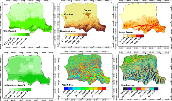
Maps of flash flood conditioning factors including: NDVI, elevation, slope, soil moisture, aspect-DEM, and flow direction
-
Elevation: Generally, there is an inverse relationship between flooding and elevation. Low-elevation areas are more susceptible to flooding (Chapi et al. 2017; Chen et al. 2019). Elevation is an important factor in flood probability (Tehrany et al. 2014b; Tien Bui et al. 2019). In this study, an elevation map with five classes was generated from the DEM (Fig. 7).
-
Slope: Various factors influence catchment hydrologic characteristics, which, in turn, affect surface runoff generation. Surface slope is a significant factor in controlling runoff (Tehrany et al. 2013). Steeper slopes have less infiltration and more runoff, while flat areas downstream of high slopes are prone to flash flooding due to excessive runoff (Li et al. 2012). In this study, a slope map with five classes was created from the DEM (Fig. 7).
-
Aspect: The aspect map shows both slope and the direction relative to the sun as significant factors in small areas. It can delineate areas near lakes and foothills with varying slopes. Flat areas are more susceptible to flooding than steep areas due to water accumulation potential (Hoang et al. 2018; Tien Bui et al. 2019). In this study, the aspect map with nine classes was derived from the DEM (Fig. 7).
-
Soil moisture: Flooding risk is also affected by saturation levels. Changes in evapotranspiration and precipitation rates impact soil moisture, limiting the ratios of infiltration, groundwater recharge, and runoff (Ahlmer et al. 2018). Several studies have found that initial soil moisture conditions can differentiate between minor and major flooding effects (Berthet et al. 2009; Brocca et al. 2008; Crow et al. 2005). Accurate and timely soil moisture content information is crucial for improving flood predictions (Kerr et al. 2010). Therefore, we processed the NASA/GLDAS/V021/NOAH/G025/T3H product in the Google Earth Engine system, implementing a programming algorithm from 2000 to 2021 to measure soil moisture (Fig. 7).
-
Flow direction: The flow direction on the elevation model indicates the potential path of water runoff. A flow direction raster was created using the depression-less DEM generated from the fill (Korah and López 2015) (Fig. 8).
Fig. 8 
Maps of flash flood conditioning factors including: distance from the road, hydrographic, distance from the river, rainfall and runoff, flow time, and geomorphology
-
River distance: The “distance from rivers” factor is crucial in determining the areas prone to flooding. Previous research has showed that areas closest to rivers are the most vulnerable to flooding (Rahmati et al. 2016). However, changes in meteorological and topographical conditions can also lead to flash floods at considerable distances from water bodies. In this study, ten buffer classes were developed at varying distances from the river (Fig. 8).
-
Rainfall and runoff: Flooding occurs in low-lying areas due to runoff formation on the land surface, primarily caused by rainfall. Runoff happens when the ground, whether soil or rock, cannot absorb abundant rainfall. Heavy, short-duration rainfall can trigger flash floods. Rainfall is the most important component in flood events (Li et al. 2012). Flooding can also result from ice melting. An annual precipitation map was developed over a 15-year period, divided into eight classes (Fig. 8).
-
Flow time: This model estimates rainfall and provides a flood alert index using only the flow scheme (Tomassetti et al. 2005) (Fig. 8).
-
Geomorphology: The understanding of dynamic landscape processes and their potential effects on natural and anthropogenic elements depends heavily on the contribution of applied geomorphology (Brandolini et al. 2008). Floods have intricated geomorphological effects on the landscape that affect it at various temporal and spatial scales. Floods influence the dynamics of geomorphic processes and shape river and valley systems (Baker 1994; Magilligan 1992). In other words, floods in a particular environment are constrained and influenced by geomorphologic controls (Křížek and Engel 2003; Poole et al. 2002). Therefore, to identify fluvial system behaviors and reduce risks, it is crucial to observe geomorphic responses in specific environments where flooding has occurred (Fig. 8).
-
Drainage density: Drainage density is an important factor in controlling the occurrence and flow of floods. Drainage characteristics such as drainage density are determined by the cumulative flow network extracted for each basin. The ratio of the total length of the hydrographic network, including both secondary and main streams, to the area of the basin, shows the drainage density. This feature indicates the condition of runoff and erosion in its various parts of the basin (Shafizadeh-Moghadam et al. 2018) (Fig. 9).
Fig. 9 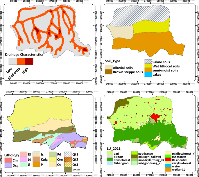
Maps of flash flood conditioning factors including: river density, soil, lithology, and land use
-
Soil: The volume of a flood is highly dependent on the type and texture of the soil. Clay soils tend to result in more rapid and significant surface runoff compared to sandy soils. Impermeable soils, mostly composed of clay, are more susceptible to flooding, whereas sandy soils are permeable and have a higher capacity to absorb surface water. Generally, the soil type can influence the amount of water that permeates the soil (Lappas and Kallioras 2019) (Fig. 9).
-
Lithology: This factor plays an important role in increasing or decreasing the occurrences of floods in a region, as it can affect the capacity for water infiltration and flood control. In the current study, lithological units were considered as one of the relevant factors (Allafta and Opp 2021). The lithology map used in this research was created using data from the Geological Survey of Iran and divided into fifteen groups (Fig. 9).
-
Land use: The intensity and severity of floods in an area are influenced by different land use types (Benito et al. 2010; García-Ruiz et al. 2008). The type of land use/land cover plays a significant role in determining the areas susceptible to floods (Norman et al. 2010). Vegetated areas are generally less vulnerable to floods, as there is an inverse relationship between vegetation and flood risk. Conversely, impervious surfaces such as residential areas, roads, and bare land increase storm runoff (Tehrany et al. 2013). The land-use/land-cover map used in this research was obtained from the Golestan Province Department of Natural Resources in 2021. The map was updated using Google Earth images and field surveys (Fig. 9).


2.4 Flood hazard potential mapping using MCDA
2.4.1 Problem description and method framework
Drawing on a geographical investigation of MCDM, this study develops a combined model for identifying flood-prone areas. The approach aims to establish interdependencies between dimensions and criteria by integrating spatial data and expert opinions. The determination of flood zones incorporates both factual geographic data (such as vegetation density, elevation, slope, soil, river distance, rainfall, drainage density, lithology, geomorphology, land use, and land cover) and value-based information (such as expert opinion, environmental characteristics, and standards). GIS is an essential tool for analyzing geographic data, as it offers robust spatial analysis capabilities. The MCDM enables the evaluation and ranking of decision options, facilitating the identification of flood-prone areas.
2.4.2 DANP multi-criteria decision analysis process
In this research, component modeling was performed using the weighted overlay method, which is considered an appropriate modeling technique. In many proportional and location analyzes, certain criteria possess greater significance and importance than others. In this method, numerical weights are assigned to each layer, and the criteria are overlapped based on their respective weights. The output layer is then influenced by the weights of the input layers. Weighting is typically performed by comparing pairs of criteria using the inputs of experts specializing in environmental sciences. The analysis involves the following steps executed in the ArcGIS software:
-
1.
Each raster or vector layer is assigned an appropriate weight for the analysis.
-
2.
The values in raster layers are classified according to the appropriate scale.
-
3.
The raster layers are stacked on top of each other, and the values of the raster pixels are multiplied by the weight of the corresponding layer. The resulting values are then summed to obtain a suitable value.
-
4.
These calculated values are written as new pixels in an output layer.
By assigning weights to each raster in the overlay process, it becomes possible to control the effect of different criteria on the model (iEsri 2022).
Based on the aforementioned points, the weight overlay method is used to multiply each sub-criterion of the main criteria by its respective weights. Subsequently, after the overlay of each criterion, the overlapping layers are multiplied by the weight of the main criterion, ultimately yielding the final output in the form of a flood map.
The DEMATEL-based ANP method was used to rank the parameters. At the descriptive level, one-dimensional tables and the DANP model were employed to rank the factors affecting flash floods.
-
Step 1: Compute the matrix of direct connections.
The relationships between the criteria, indicating the impact of one criterion on another, are determined using the opinions of decision makers. These relationships are rated on a numerical scale from 0 to 4, representing the following levels of impact: 0 (no impact), 1 (low impact), 2 (moderate impact), 3 (high impact), and 4 (very high impact). In this step, the average opinion of the experts is computed.
-
Step 2: Normalize the direct relationship matrix
The direct communication matrix D is obtained using the following normalization relation and the N matrix.
-
Step 3: Compute the criteria's entire communication matrix
After normalizing matrix D and obtaining matrix N, the entire communication matrix can be computed using the provided equation, which involves the unit matrix.
-
Step 4: Compute the total correlation matrix of the parameters and determine the severity and direction of influence
First, the total correlation matrix is generated from the complete correlation matrix of the Tc criterion. As a result, every matrix element is computed by taking the average of the components in the doors:

Formulas 6, 7, and 8, are used to separately compute the sum of rows and columns of the total correlation matrix:
The indices \({r}_{i}\) and \({c}_{j}\) represent the sums of the i-th row and j-th column, respectively. The index \({{r}}_{{i}}+{{c}}_{{j}}\) indicates the significance (intense) of the i-th criterion, while \({r}_{i}-{c}_{j}\) indicates the effectiveness or influence of criterion i. When \({r}_{i}-{c}_{j}\) is positive (i = j), criterion i is one of the causative or influencing factors. When \({r}_{i}-{c}_{j}\) is negative (i = j), criterion i is one of the impressionable factors. Similarly, the weights of indices R and C are computed. The index Ri shows the sum of the i-th row, and the index Cj represents the sum of the j-th column of the TD matrix.
-
Step 5: Normalize the full relational dimension matrix (\({T}_{D}^{\propto }\))
The matrix \({T}_{D}^{\propto }\) is normalized by calculating each row and dividing each element by the sum of elements in its respective row. Finally, the row and column of the obtained matrix are replaced.
-
Step 6: Normalize the criteria for total correlation of criteria
This step involves computing the sums of rows, dividing each element by the sum of elements in its own row, and performing normalization using the provided formulas:

-
Step 7: Formation of unweighted w matrix
To obtain the matrix w, the displacement matrix is entirely normalized. An empty or zero matrix indicates that the criteria are independent.

-
Step 8: Formation of a weighted supermatrix
The complete normalized communication matrix is transposed and multiplied by the unweighted supermatrix to form the weighted supermatrix.
-
Step 9: Limit the weighted supermatrix
To ensure stability and convergence of the supermatrix, it is necessary to limit the weighted supermatrix until a significant value of z is reached. This process yields effective DANP weights for the results (Chiu et al. 2013).
Due to the complexity and potential for computational errors, it is advisable to use software such as Matlab to facilitate the matrix operations. In this research, Matlab software was used to limit the weight matrix. The process involved designing and preparing the initial Dematel matrix, criteria, and sub-criteria in an Excel file using a Matlab processing code. This programmed analytical code encompasses the steps of the combined DANP method.
The initial processing was performed, and the outputs were calculated and stored in a file. This file includes various matrices such as normal matrix, TC matrix or general communication, normalized TC, primary supermatrix, TD matrix, normalized TD, and weighted decision matrix.
In the second stage, the final weighted matrix needs to reach an appropriate power for convergence. To accomplish this, the generated matrix is prepared as an Excel file. Subsequently, the Matlab file is used to conduct convergence analysis by iteratively adjusting the numbers until they reach an accuracy of 0.00005. In other words, when the difference between two consecutive numbers becomes smaller than this threshold, the output is printed. The power of 3 is applied during this analysis. Finally, the final weights and prioritization of each sub-criterion are extracted.
3 Results
Floods are a significant and recurrent natural hazard in Iran. The identification and delineation of flood-prone areas play a crucial role in flood risk management. Flood risk zoning enables a quantitative assessment of flood risk, and evaluation is essential for the development and quality assessment of flood risk zoning maps. Among the various factors influencing flood zoning, rivers and water bodies such as lakes act as natural barriers and are of utmost importance. Their shape, natural characteristics, pathways, width, depth, and intensity significantly affects the distribution patterns of floods.
In this study, twelve criteria were identified to achieve the research objectives, encompassing meteorological, geomorphological, hydrological, geophysical, and geographical aspects. These criteria were integrated within a GIS environment to generate the final flood susceptibility maps. To acquire objective information and comprehensive insights into the study region, a questionnaire was designed and administered to gather data for the criteria lacking registered and official information. A total of 15 specialists and experts in the field, along with 20 local managers, were involved in completing the questionnaire. Their extensive knowledge of the region ensured the provision of accurate and unbiased information, enabling a thorough review and analysis of the research.
The DEMATEL and ANP methodologies were employed, incorporating the insights and opinions of the reviewed experts. The relative importance and interdependencies of the criteria were determined through pairwise comparisons conducted by the experts, as presented in Tables 2, 3, 4, 5, and 6. The final weights of the main factors were reclassified from fuzzy comparison according to their importance, as outlined in Table 7.
Based on the final weights, topography emerges as the most influential factor contributing to flood risk in this area. The topography of a region undoubtedly plays a significant role in shaping the flow and accumulation of water, as well as the speed and direction of floods. Steep slopes, narrow valleys, and canyons facilitate the rapid collection and forceful movement of water, rendering these areas more susceptible to flash floods. Moreover, the type of surface and vegetation cover present in a region can impact the intensity of flash floods. Regions characterized by impervious surfaces such as concrete or asphalt tend to experience greater runoff and faster flooding compared to areas with permeable surfaces like grass or forests, which have the ability to absorb and regulate the flow of water. Consequently, land use and vegetation density were identified as the second weighting factors influencing flood dynamics. Following these, the hydrographic, soil and geology, and climatic factors, respectively, contribute to the flood characteristics in the region.
The overall findings indicate that the northern part of the study area is at higher risk of flooding compared to the southern part. Approximately 62.39% of the northern and middle part of the watershed have a slope ranging from zero to 5 degrees. Additionally, around 33.64% of these areas are located within 100 m of the river, which indicates a high-risk zone. These regions receive approximately 37% of the total rainfall, which is 450 mm.
The central part of the watershed, comprising about 62.28% of the area, is situated at an altitude ranging from 1130 to 1500 m. This central region is characterized by a predominantly flat terrain with a significant lack of vegetation cover. Due to its proximity to the river and the considerable amount of rainfall it receives, these factors collectively contribute to increased rainfall, river flooding, and subsequent runoff.
After applying weights to the suitability classes and criteria, the individual layers were combined, resulting in the preparation of a final suitability map. The obtained results were then presented. Figure 10 depicts the final map, which highlights unfavorable areas and facilitates better control and planning of flood-related crises. It can be inferred that a majority of the villages are situated within one kilometer of the river, where the flood intensity is particularly high. This indicates that most rural settlements in the Qarasu watershed are highly susceptible to flooding, particularly during events of maximum intensity. The zoning analysis also reveals that out of the total 134 villages in the Qarasu basin, 31 villages are classified as high-risk, 17 villages fall under the moderate-risk category, and 20 villages are located in low-risk areas, representing 50% of all the villages in the basin. According to the zoning outcomes, approximately 83,595 individuals residing in rural areas within this catchment area are exposed to the risk of flash flooding.

Threshold of flood risk in the Qarasu watershed
4 Discussion
4.1 Flash flood analysis and method validation
Many studies have examined the reasons behind people's decision to reside in crisis-prone areas, focusing on the dangers of floods, hurricanes, earthquakes, and other devastating climatic and environmental disasters. These studies also explore how individuals perceive and understand the associated risks. Most research in this field has primarily focused on physical and financial losses, as well as human aspects and casualties (Berkes 2007). Notably, in 1989, the United Nations General Assembly presented the International Risk Reduction Program, declaring the 1990s as the International Decade for Natural Disaster Reduction. The primary objective of this initiative was to reduce the loss of life and property, as well as mitigate the devastating effects of natural disasters through social and economic efforts. Environmental hazards, including earthquakes, hurricanes, tsunamis, floods, and other natural disasters, were the key focus (The Energy and Resources Institute 2006).
Since then, extensive research has been conducted on natural hazards and strategies to reduce their detrimental impacts, mainly through the approaches of "reducing vulnerability" and "increasing resilience." It is worth noting that most of these studies have focused on urban areas, emphasizing crisis management and urban planning, while research specifically related to rural areas remains limited. However, considering that global and Iranian experiences in urban planning studies can also contribute to rural research, a detailed discussion on the research background at both national and international levels will be presented.
Today, one of the most effective aspects of flood damage management and reduction is providing information and raising awareness among the public (Kellens et al. 2011). It is widely accepted within the scientific community that extreme natural hazards like floods cannot be entirely prevented. However, through efficient flood susceptibility modeling, a significant portion of human lives and socio-economic impacts can be mitigated (Khosravi et al. 2019). Therefore, access to flood vulnerability maps can help managers obtain pertinent information about flood-risk areas and making informed decisions.
Several researchers argue that the MCDM methodology has advantages over other techniques that rely on historical and reliable data. It plays a crucial role in effectively identifying, integrating, or ranking factors in natural hazard assessment (Sahraei et al. 2022). Compared to other MCDM approaches, the DEMATEL-ANP method proves to be efficient in solving decision-making problems. The key benefit of this hybrid approach is its ability to identify the most critical components influencing flash flood risk, from a complicated multi-criteria decision structure, by converting the causal relationship between decision criteria's interdependency into matrices (Ali et al. 2020). The analysis of both direct and indirect relationships between these factors allows for a more comprehensive understanding of flash flood risk. Furthermore, the use of satellite data can provide additional information on the characteristics of specific areas and historical information that can be used to identify patterns and trends in flash flood risk.
In network analysis, evaluating the validity and consistency of pairwise comparisons is crucial as it enhances our knowledge of network analysis, component interactions, and prioritization for improved decision-making (Ozdemir 2005). Considering the inherent uncertainty associated with expert judgments in determining the importance and influence of conditional factors, the combination of the DEMATEL-ANP method has demonstrated high accuracy in flood susceptibility assessment. For example, a research conducted by Ali Azareh et al.’s in the Haraz watershed in Iran, with an accuracy of approximately 89% (Azareh et al. 2021). The ANP method that calculates interdependence between factors through network analysis, when combined with the DEMATEL method, allows for the determination and filling of gaps in understanding the interdependencies between factors, thereby facilitating well-documented flood vulnerability analysis (Hosseini et al. 2021). This approach has been effectively utilized by planners, as demonstrated in Manas Mondal et al.'s research on assessing the risks of severe hydro-climatic events, such as coastal flooding in the West Bengal delta in India. Similarly, Ali et al. used this method to assess flood susceptibility in the Topla basin in Slovakia, with their research reporting a high accuracy of 92% (Ali et al. 2020).
However, it is important to acknowledge the limitations of the discussed method. Mahmoud and Gan (2018) suggested that at least six weighted factors should be considered to avoid overestimation of certain factors. The accuracy of satellite data can vary depending on resolution and sensor quality, and its availability may be limited in some regions. Furthermore, the approach assumes fixed and known relationships between factors, which may not hold true in reality as these relationships may change over time, potentially reducing the accuracy of the approach. Thus, the risk assessment should be continuously updated and validated with new data, and the approach should be used as a decision-making tool rather than an absolute truth. Another limitation is the temporal aspect of flood vulnerability, which was not considered in the present research focused on spatial flood susceptibility analysis (Azareh et al. 2021). Future studies in flood modeling should address this limitation.
4.2 Relationship between flood hazard and planning
The relationship between flood hazard and planning is an important issue to discuss, particularly because many parts of the world are experiencing an increase in the frequency and severity of floods due to climate change (Wilson and Chakraborty 2013). Climate change will have the greatest impact on the future evolution of floods, influenced by numerous other factors, including the human factor. However, estimating its trend can be challenging due to the numerous influencing factors. The accuracy of current global flood risk projections is constrained due to these complex factors. Therefore, accurate analysis and modeling of floods can greatly aid in forward-thinking and planning (Mezősi 2022). In order to develop efficient flood management measures, planners must have a complete grasp of the flood threat in their region. Once flood-prone areas are determined, this knowledge can guide decisions on land use planning and development.
Planning can also help reduce the likelihood of flooding in previously established areas. This could entail taking steps like constructing levees or flood barriers, installing retention ponds or other drainage infrastructure, or upgrading structures to be more flood-resistant (Bathrellos et al. 2016, 2018). In flood-prone areas, runoff is often intense, resulting in more severe damage due to restricted infiltration. Hence, the construction and routine maintenance of drainage systems with sufficient cross sections are required in impacted settlements. In mountainous enclosed valleys where flood prevention levees are typically absent, the use of mobile dams has been successful in many cases since the early 2000s (Mezősi 2022). Careful land use planning and proper building design are crucial in flood-prone areas to prevent and minimize the impact of flood hazards. This practical approach can be applied to both new and existing land use planning projects, as well as floodplain control. Flood spreading is a technique used to manage water resources in areas that receive low rainfall. It involves capturing floodwaters and diverting them to low-lying areas where they can be stored in the soil or used for groundwater recharge. This technique is particularly effective in arid and semi-arid areas where water is scarce and where the risk of flash flooding is high (Ziaiian Firouz Abadi et al. 2020).
Wherefore, before a flood affects a community, the local mayor holds the position of authority and has the power and authority to determine if an emergency has occurred based on the expertly prepared results and information from the early warning system.
In a book titled "Cooperation with Nature: Dealing with Natural Hazards with Land Use Planning for Sustainable Communities," which is divided into three general parts, the authors aim to present a comprehensive vision of sustainable societies and provide suggestions for reforming policies and planning methods (Burby 1998). The research findings show that local governments should use land use management tools to carry out comprehensive plans. By predicting and handling risk reduction programs, they can provide a basis for achieving the goals of risk reduction and enhancing community resilience in the face of disasters and natural hazards. Accordingly, community engagement is necessary for successful flood planning to ensure that their needs and concerns are considered. This may involve stakeholder consultations, public education, and outreach initiatives to develop flood management strategies that align with the community's requirements.
Overall, the relationship between flood hazard and planning is vital to ensure that communities can manage flood risks. By incorporating flood hazard information into planning processes and actively engaging with the community, planners can contribute to the development of more resilient and sustainable communities that are better equipped to withstand the impacts of climate change.
5 Conclusion and recommendations
Decision-making (DANP) integration with GIS and remote sensing could serve as an efficient method for zoning flash flood-risk areas. This approach allows decision-makers to investigate and assess multiple factors that impact the incidence and severity of flash floods. Based on the final weights obtained, topography was found to have the greatest impact on flood risk in the area. Undoubtedly, the topography of an area can significantly influence the flow and accumulation of water, as well as the speed and direction of the flood. Steep slopes, narrow valleys, and canyons can facilitate the rapid and forceful collection of water, making these areas more vulnerable to flash floods. Additionally, the type of surface and vegetation cover in a region can affect the intensity of flash floods. Regions with impervious surfaces such as concrete or asphalt may experience higher runoff and faster floods than regions with permeable surfaces such as grass or forested areas, which can absorb and moderate the flow of water. For this reason, land use and vegetation density were chosen as the second weighting factor influencing flood risk. Subsequently, hydrographic, soil and geology, climatic were identified as the factors affecting flood in the region, respectively.
The purpose of this research was to evaluate the main factors contributing to flash floods and identify hotspots and vulnerable populations. The general results of the flood intensity map in the Qarasu watershed indicate that most villages are located within one kilometer of the river, with high flood intensity. In other words, the majority of rural settlements in the Qarasu watershed are at a high risk of flooding with maximum intensity, significantly increasing the likelihood of damage and casualties due to flash floods. During heavy rainfall, the river can overflow its banks and inundate nearby areas, causing extensive damage to infrastructure and posing risks to lives. Based on the authors’ knowledge from numerous field visits, most of the lands within a one-kilometer distance from the river are used for agricultural purposes. This land use pattern can increase the risk of flooding due to reduced water absorption and increased runoff. Furthermore, due to the development of facilities for the dynamism of the villages in this region, the population has grown, and many lands have undergone changes in land use. As a result, the flooding of these villages causes more damage and leads to the disruption of vital infrastructures such as health centers, schools, and existing power plants in the area. According to the zoning, out of 134 villages in the Qarasu basin, 31 villages are classified as high-risk, 17 villages as moderate-risk, and 20 villages as low-risk areas (which account for 50% of all villages in this basin). Consequently, approximately 83,595 rural residents in this catchment area are at risk of flash flooding.
For future research, it is necessary to examine the resilience of people living in flood-prone areas. Specifically, the relationship between environmental–physical factors in the risk points of the Qarasu watershed (such as the quality of constructions, materials, and building standards, etc.) and the resilience of communities facing floods needs to be determined. Furthermore, it is important to identify the connection between economic factors in the Qarasu watershed communities (such as type of job, income levels, capitals, and assets) and their level of resilience against floods.
To enhance crisis management in the study area, based on the materials provided, it is recommended to conduct more comprehensive studies on the flood potential of the basin by involving more stakeholders and layers of analysis. In the northern and central parts of the watershed, efforts should be made to plant vegetation in the natural environment and prevent construction in the riverbed. The flood susceptibility model developed in this study can serve as a valuable resource for future research and can contribute to promoting the integration of GIS-based DANP and remote sensing techniques. This, in turn, may foster the development and application of hybrid strategies to further enhance flood forecasting and management practices. In comparison to other integrated approaches, there is currently limited published literature on the application of the DANP and GIS-based DANP model, highlighting the potential for further research and exploration in this field.
Code availability
The code used for the scenario analyses is available from the corresponding author on request.
References
Ahlmer A-K, Cavalli M, Hansson K, Koutsouris AJ, Crema S, Kalantari Z (2018) Soil moisture remote-sensing applications for identification of flood-prone areas along transport infrastructure. Environ Earth Sci 77:1–17. https://doi.org/10.1007/s12665-018-7704-z
Ali SA, Parvin F, Pham QB, Vojtek M, Vojteková J, Costache R, Linh NTT, Nguyen HQ, Ahmad A, Ghorbani MA (2020) GIS-based comparative assessment of flood susceptibility mapping using hybrid multi-criteria decision-making approach, naïve Bayes tree, bivariate statistics and logistic regression: a case of Topľa basin, Slovakia. Ecol Indicators 117:106620. https://doi.org/10.1016/j.ecolind.2020.106620
Allafta H, Opp C (2021) GIS-based multi-criteria analysis for flood prone areas mapping in the trans-boundary Shatt Al-Arab basin, Iraq-Iran. Geomat Nat Haz Risk 12:2087–2116. https://doi.org/10.1080/19475705.2021.1955755
Arabsheibani R, Kanani Sadat Y, Abedini A (2016) Land suitability assessment for locating industrial parks: a hybrid multi criteria decision-making approach using Geographical Information System. Geogr Res 54:446–460. https://doi.org/10.1111/1745-5871.12176
Azareh A, Rafiei Sardooi E, Choubin B, Barkhori S, Shahdadi A, Adamowski J, Shamshirband S (2021) Incorporating multi-criteria decision-making and fuzzy-value functions for flood susceptibility assessment. Geocarto Int 36:2345–2365. https://doi.org/10.1080/10106049.2019.1695958
Azizi A, Malekmohammadi B, Jafari HR, Nasiri H, Amini Parsa V (2014) Land suitability assessment for wind power plant site selection using ANP-DEMATEL in a GIS environment: case study of Ardabil province. Iran Environ Monit Assess 186:6695–6709. https://doi.org/10.1007/s10661-014-3883-6
Badraq Nejad A, Sarli R, Babaii M, Basiri M (2019) Evaluating and analyzing the spatial distribution of rural inhabitants with emphasis on biological and activity risk taking using GIS and SPSS (the area under study: Aq Su rural area). J Stud Human Settlements Plan 14:735–756
Baker VR (1994) Geomorphological understanding of floods. In: Geomorphology and natural hazards. Elsevier, Amsterdam, pp 139–156.
Bathrellos G, Karymbalis E, Skilodimou H, Gaki-Papanastassiou K, Baltas E (2016) Urban flood hazard assessment in the basin of Athens Metropolitan city, Greece. Environ Earth Sci 75:1–14
Bathrellos GD, Skilodimou HD, Soukis K, Koskeridou E (2018) Temporal and spatial analysis of flood occurrences in the drainage basin of pinios river (thessaly, central greece). Land 7:106. https://doi.org/10.3390/land7030106
Benito G, Rico M, Sánchez-Moya Y, Sopeña A, Thorndycraft V, Barriendos M (2010) The impact of late Holocene climatic variability and land use change on the flood hydrology of the Guadalentín River, southeast Spain. Global Planet Change 70:53–63. https://doi.org/10.1016/j.gloplacha.2009.11.007
Berkes F (2007) Understanding uncertainty and reducing vulnerability: lessons from resilience thinking. Nat Hazards 41:283–295. https://doi.org/10.1007/s11069-006-9036-7
Berthet L, Andréassian V, Perrin C, Javelle P (2009) How crucial is it to account for the antecedent moisture conditions in flood forecasting? Comparison of event-based and continuous approaches on 178 catchments. Hydrol Earth Syst Sci 13:819–831. https://doi.org/10.5194/hess-13-819-2009
Brandolini P, Faccini F, Robbiano A, Terranova R (2008) Relationship between flood hazards and geomorphology applied to land planning in the upper Aveto Valley (Liguria, Italy). Geogr Fis Din Quat 31:73–82
Brocca L, Melone F, Moramarco T (2008) On the estimation of antecedent wetness conditions in rainfall–runoff modelling. Hydrol Process Int J 22:629–642. https://doi.org/10.1002/hyp.6629
Burby RJ (1998) Cooperating with nature: Confronting natural hazards with land-use planning for sustainable communities. Joseph Henry Press, USA
Büyüközkan G, Güleryüz S (2016) An integrated DEMATEL-ANP approach for renewable energy resources selection in Turkey. Int J Prod Econ 182:435–448. https://doi.org/10.1016/j.ijpe.2016.09.015
Chapi K, Singh VP, Shirzadi A, Shahabi H, Bui DT, Pham BT, Khosravi K (2017) A novel hybrid artificial intelligence approach for flood susceptibility assessment. Environ Model Softw 95:229–245. https://doi.org/10.1016/j.envsoft.2017.06.012
Chen W, Hong H, Li S, Shahabi H, Wang Y, Wang X, Ahmad BB (2019) Flood susceptibility modelling using novel hybrid approach of reduced-error pruning trees with bagging and random subspace ensembles. J Hydrol 575:864–873. https://doi.org/10.1016/j.jhydrol.2019.05.089
Chiu W-Y, Tzeng G-H, Li H-L (2013) A new hybrid MCDM model combining DANP with VIKOR to improve e-store business. Knowl-Based Syst 37:48–61. https://doi.org/10.1016/j.knosys.2012.06.017
Chukwuma E, Okonkwo C, Ojediran J, Anizoba D, Ubah J, Nwachukwu C (2021) A GIS based flood vulnerability modelling of Anambra State using an integrated IVFRN-DEMATEL-ANP model. Heliyon 7:e08048. https://doi.org/10.1016/j.heliyon.2021.e08048
Convertino M, Annis A, Nardi F (2019) Information-theoretic portfolio decision model for optimal flood management. Environ Model Softw 119:258–274. https://doi.org/10.1016/j.envsoft.2019.06.013
Crow WT, Bindlish R, Jackson TJ (2005) The added value of spaceborne passive microwave soil moisture retrievals for forecasting rainfall‐runoff partitioning. Geophys Res Lett 32. https://doi.org/10.1029/2005GL023543
Ekmekcioğlu Ö, Koc K, Özger M (2022) Towards flood risk mapping based on multi-tiered decision making in a densely urbanized metropolitan city of Istanbul. Sustain Cities Soc 80:103759
iEsri. 2022. ArcGIS Desktop: Release 10.5. In.
Franci F, Bitelli G, Mandanici E, Hadjimitsis D, Agapiou A (2016) Satellite remote sensing and GIS-based multi-criteria analysis for flood hazard mapping. Nat Hazards 83:31–51. https://doi.org/10.1007/s11069-016-2504-9
García-Ruiz JM, Regüés D, Alvera B, Lana-Renault N, Serrano-Muela P, Nadal-Romero E, Navas A, Latron J, Martí-Bono C, Arnáez J (2008) Flood generation and sediment transport in experimental catchments affected by land use changes in the central Pyrenees. J Hydrol 356:245–260. https://doi.org/10.1016/j.jhydrol.2008.04.013
Gigović L, Pamučar D, Božanić D, Ljubojević S (2017) Application of the GIS-DANP-MABAC multi-criteria model for selecting the location of wind farms: a case study of Vojvodina, Serbia. Renew Energy 103:501–521. https://doi.org/10.1016/j.renene.2016.11.057
Hapuarachchi H, Wang Q, Pagano T (2011) A review of advances in flash flood forecasting. Hydrol Process 25:2771–2784. https://doi.org/10.1002/hyp.8040
Haq M, Akhtar M, Muhammad S, Paras S, Rahmatullah J (2012) Techniques of remote sensing and GIS for flood monitoring and damage assessment: a case study of Sindh province, Pakistan. The Egyptian J Remote Sens Space Sci 15:135–141. https://doi.org/10.1016/j.ejrs.2012.07.002
Harsha J, Ravikumar A, Shivakumar B (2020) Evaluation of morphometric parameters and hypsometric curve of Arkavathy river basin using RS and GIS techniques. Appl Water Sci 10:1–15. https://doi.org/10.1007/s13201-020-1164-9
He B, Huang X, Ma M, et al (2018) Analysis of flash flood disaster characteristics in China from 2011 to 2015. Nat Haz 90:407–420. https://doi.org/10.1007/s11069-017-3052-7
Hoang LP, Biesbroek R, Tri VPD, Kummu M, van Vliet MT, Leemans R, Kabat P, Ludwig F (2018) Managing flood risks in the Mekong Delta: How to address emerging challenges under climate change and socioeconomic developments. Ambio 47:635–649. https://doi.org/10.1007/s13280-017-1009-4
Hosseini FS, Sigaroodi SK, Salajegheh A, Moghaddamnia A, Choubin B (2021) Towards a flood vulnerability assessment of watershed using integration of decision-making trial and evaluation laboratory, analytical network process, and fuzzy theories. Environ Sci Pollut Res 28:62487–62498. https://doi.org/10.1007/s11356-021-14534-w
Kanani-Sadat Y, Arabsheibani R, Karimipour F, Nasseri M (2019) A new approach to flood susceptibility assessment in data-scarce and ungauged regions based on GIS-based hybrid multi criteria decision-making method. J Hydrol 572:17–31. https://doi.org/10.1016/j.jhydrol.2019.02.034
Kazakis N, Kougias I, Patsialis T (2015) Assessment of flood hazard areas at a regional scale using an index-based approach and Analytical Hierarchy Process: application in Rhodope-Evros region, Greece. Sci Total Environ 538:555–563. https://doi.org/10.1016/j.scitotenv.2015.08.055
Kellens W, Zaalberg R, Neutens T, Vanneuville W, De Maeyer P (2011) An analysis of the public perception of flood risk on the Belgian coast. Risk Anal Int J 31:1055–1068. https://doi.org/10.1111/j.1539-6924.2010.01571.x
Kerr YH, Waldteufel P, Wigneron J-P, Delwart S, Cabot F, Boutin J, Escorihuela M-J, Font J, Reul N, Gruhier C (2010) The SMOS mission: New tool for monitoring key elements ofthe global water cycle. Proc IEEE 98:666–687. https://doi.org/10.1109/JPROC.2010.2043032
Khosravi K, Shahabi H, Pham BT, Adamowski J, Shirzadi A, Pradhan B, Dou J, Ly H-B, Gróf G, Ho HL (2019) A comparative assessment of flood susceptibility modeling using multi-criteria decision-making analysis and machine learning methods. J Hydrol 573:311–323. https://doi.org/10.1016/j.jhydrol.2019.03.073
Korah PI, López FMJ (2015) Mapping Flood Vulnerable Areas in Quetzaltenango, Guatemala using GIS. J Environ Earth Sci 5:132–143
Křížek M, Engel Z (2003) Geomorphological consequences ot the 2002 flood in the Otava river drainage basin.
Lappas I, Kallioras A (2019) Flood susceptibility assessment through GIS-based multi-criteria approach and analytical hierarchy process (AHP) in a river basin in Central Greece. Int Res J Eng Technol.
Layomi Jayasinghe S, Kumar L, Sandamali J (2019) Assessment of potential land suitability for tea (Camellia sinensis (L.) O. Kuntze) in Sri Lanka using a GIS-based multi-criteria approach. Agriculture 9:148. https://doi.org/10.3390/agriculture9070148
Li K, Wu S, Dai E, Xu Z (2012) Flood loss analysis and quantitative risk assessment in China. Nat Hazards 63:737–760. https://doi.org/10.1007/s11069-012-0180-y
Magilligan FJ (1992) Thresholds and the spatial variability of flood power during extreme floods. Geomorphology 5:373–390. https://doi.org/10.1016/0169-555X(92)90014-F
Mahmoud SH, Gan TY (2018) Multi-criteria approach to develop flood susceptibility maps in arid regions of Middle East. J Clean Prod 196:216–229. https://doi.org/10.1016/j.jclepro.2018.06.047
Malczewski J (2006) GIS-based multicriteria decision analysis: a survey of the literature. Int J Geogr Inf Sci 20:703–726. https://doi.org/10.1080/13658810600661508
Malmir M, Zarkesh MMK, Monavari SM, Jozi SA, Sharifi E (2016) Analysis of land suitability for urban development in Ahwaz County in southwestern Iran using fuzzy logic and analytic network process (ANP). Environ Monit Assess 188:1–23. https://doi.org/10.1007/s10661-016-5401-5
Mamashli Z, Nayeri S, Tavakkoli-Moghaddam R, Sazvar Z, Javadian N (2021) Designing a sustainable–resilient disaster waste management system under hybrid uncertainty: a case study. Eng Appl Artif Intell 106:104459. https://doi.org/10.1016/j.engappai.2021.104459
Masoudi E, Hedayati A, Bagheri T, Salati A, Safari R, Gholizadeh M, Zakeri M (2022) Different land uses influenced on characteristics and distribution of microplastics in Qarasu Basin Rivers, Gorgan Bay, Caspian Sea. Environ Sci Pollut Res 29:64031–64039. https://doi.org/10.1007/s11356-022-20342-7
Memon AA, Muhammad S, Rahman S, Haq M (2015) Flood monitoring and damage assessment using water indices: A case study of Pakistan flood-2012. Egyptian J Remote Sens Space Sci 18:99–106. https://doi.org/10.1016/j.ejrs.2015.03.003
Mezősi G (2022). Natural hazards and the mitigation of their impact. Springer. https://doi.org/10.1007/978-3-031-07226-0
Nguyen-Huy T, Kath J, Nagler T, Khaung Y, Aung TSS, Mushtaq S, Marcussen T, Stone R (2022) A satellite-based Standardized Antecedent Precipitation Index (SAPI) for mapping extreme rainfall risk in Myanmar. Remote Sens Appl Soc Environ, p 100733.
Norman LM, Huth H, Levick L, Shea Burns I, Phillip Guertin D, Lara-Valencia F, Semmens D (2010) Flood hazard awareness and hydrologic modelling at Ambos Nogales, United States-Mexico border. J Flood Risk Manage 3:151–165. https://doi.org/10.1111/j.1753-318X.2010.01066
Orimoloye IR, Belle JA, Ololade OO (2021) Drought disaster monitoring using MODIS derived index for drought years: a space-based information for ecosystems and environmental conservation. J Environ Manage 284:112028. https://doi.org/10.1016/j.jenvman.2021.112028
Ozdemir MS (2005) Validity and inconsistency in the analytic hierarchy process. Appl Math Comput 161:707–720. https://doi.org/10.1016/j.amc.2003.12.099
Patel DP, Srivastava PK (2013) Flood hazards mitigation analysis using remote sensing and GIS: correspondence with town planning scheme. Water Resour Manage 27:2353–2368. https://doi.org/10.1007/s11269-013-0291-6
Poole GC, Stanford JA, Frissell CA, Running SW (2002) Three-dimensional mapping of geomorphic controls on flood-plain hydrology and connectivity from aerial photos. Geomorphology 48:329–347. https://doi.org/10.1016/S0169-555X(02)00078-8
Pradhan B, OHb H-J, Buchroithner M (2010) Use of remote sensing data and GIS to produce a landslide susceptibility map of a landslide prone area using a weight of evidence model. Assessment 11:13.
Prasad R, Charan D, Joseph L, Nguyen-Huy T, Deo RC, Singh S (2021) Daily flood forecasts with intelligent data analytic models: multivariate empirical mode decomposition-based modeling methods. In: Intelligent data analytics for decision-support systems in hazard mitigation. Springer, Cham, pp 359–381.
Rahmati O, Zeinivand H, Besharat M (2016) Flood hazard zoning in Yasooj region, Iran, using GIS and multi-criteria decision analysis. Geomat Nat Haz Risk 7:1000–1017. https://doi.org/10.1080/19475705.2015.1045043
Ren H, Zou X, Zhang P (2007) An elementary study on causing-factors of Chinese mountain torrents disaster. China Water Resour 14:18–20
Saaty TL (2004) Fundamentals of the analytic network process—dependence and feedback in decision-making with a single network. J Syst Sci Syst Eng 13:129–157. https://doi.org/10.1007/s11518-006-0158-y
Sadeghi-Pouya A, Nouri J, Mansouri N, Kia-Lashaki A (2017) Developing an index model for flood risk assessment in the western coastal region of Mazandaran. Iran J Hydrol Hydromech 65:134–145. https://doi.org/10.1515/johh-2017-0007
Sahraei R, Kanani‐Sadat Y, Homayouni S, Safari A, Oubennaceur K, Chokmani K (2022) A novel hybrid GIS‐based multi‐criteria decision‐making approach for flood susceptibility analysis in large ungauged watersheds. J Flood Risk Manage, p e12879. https://doi.org/10.1111/jfr3.12879
Seyedmohammadi J, Sarmadian F, Jafarzadeh AA, McDowell RW (2019) Integration of ANP and Fuzzy set techniques for land suitability assessment based on remote sensing and GIS for irrigated maize cultivation. Arch Agron Soil Sci 65:1063–1079. https://doi.org/10.1080/03650340.2018.1549363
Shafizadeh-Moghadam H, Valavi R, Shahabi H, Chapi K, Shirzadi A (2018) Novel forecasting approaches using combination of machine learning and statistical models for flood susceptibility mapping. J Environ Manage 217:1–11. https://doi.org/10.1016/j.jenvman.2018.03.089
Shahiri Tabarestani E, Afzalimehr H (2021) Artificial neural network and multi-criteria decision-making models for flood simulation in GIS: Mazandaran Province, Iran. Stochastic Environ Res Risk Assessment, pp 1–19. https://doi.org/10.1007/s00477-021-01997-z
Sharifi F, Samadi SZ, Wilson CA (2012) Causes and consequences of recent floods in the Golestan catchments and Caspian Sea regions of Iran. Nat Hazards 61:533–550. https://doi.org/10.1007/s11069-011-9934-1
Taherizadeh M, Khushemehr JH, Niknam A, Nguyen-Huy T, Mezosi G (2023) Revealing the effect of an industrial flash flood on vegetation area: a case study of Khusheh Mehr in Maragheh-Bonab Plain, Iran. Society and Environment, Remote Sensing Applications
Tehrany MS, Lee M-J, Pradhan B, Jebur MN, Lee S (2014a) Flood susceptibility mapping using integrated bivariate and multivariate statistical models. Environ Earth Sci 72:4001–4015. https://doi.org/10.1007/s12665-014-3289-3
Tehrany MS, Pradhan B, Jebur MN (2013) Spatial prediction of flood susceptible areas using rule based decision tree (DT) and a novel ensemble bivariate and multivariate statistical models in GIS. J Hydrol 504:69–79. https://doi.org/10.1016/j.jhydrol.2013.09.034
Tehrany MS, Pradhan B, Jebur MN (2014b) Flood susceptibility mapping using a novel ensemble weights-of-evidence and support vector machine models in GIS. J Hydrol 512:332–343. https://doi.org/10.1016/j.jhydrol.2014.03.008
Teniwut W, Marimin M, Djatna T (2019) GIS-Based multi-criteria decision making model for site selection of seaweed farming information centre: a lesson from small islands, Indonesia. Decis Sci Lett 8:137–150. https://doi.org/10.5267/j.dsl.2018.8.001
The Energy and Resources Institute (2006) Adaptation to Climate Change in the Context of Sustainable Development. In: Climate Change and Sustainable Development: A Workshop to Strengthen Research and Understanding, New Delhi, 7–8 April
Tien Bui D, Shirzadi A, Shahabi H, Chapi K, Omidavr E, Pham BT, Talebpour Asl D, Khaledian H, Pradhan B, Panahi M (2019) A novel ensemble artificial intelligence approach for gully erosion mapping in a semi-arid watershed (Iran). Sensors 19:2444
Tomassetti B, Coppola E, Verdecchia M, Visconti G (2005) Coupling a distributed grid based hydrological model and MM5 meteorological model for flooding alert mapping. Adv Geosci 2:59–63. https://doi.org/10.5194/adgeo-2-59-2005
Trivedi A (2018) A multi-criteria decision approach based on DEMATEL to assess determinants of shelter site selection in disaster response. Int J Disast Risk Reduct 31:722–728. https://doi.org/10.1016/j.ijdrr.2018.07.019
Vafaie F, Hadipour A, Hadipour V (2015) Gis-based fuzzy multi-criteria decision making model for coastal aquaculture site selection. Environ Eng Manage J (EEMJ) 14. https://doi.org/10.30638/eemj.2015.258
Wilson B, Chakraborty A (2013) The environmental impacts of sprawl: Emergent themes from the past decade of planning research. Sustainability 5:3302–3327. https://doi.org/10.3390/su5083302
Ziaiian Firouz Abadi P, Badragh Nejad A, Sarli R, Babaie M (2020) Measurement and identification of areas susceptible to flood spreading from the viewpoint of geological formations in Birjand watershed using RS/GIS. J Appl Res Geograph Sci 20:1–24. https://doi.org/10.29252/jgs.20.57.1
Funding
Open access funding provided by University of Szeged. The authors declare that no funds, grants, or other support were received during the preparation of this manuscript.
Author information
Authors and Affiliations
Contributions
MT contributed to conceptualization, methodology, analysis, validation, writing original preparation and software. AN contributed to writing, methodology, discussion, and software. TN-H contributed to supervision, writing-reviewing and editing. GM contributed to supervision, writing-reviewing and editing. RS contributed to data curation, writing-review and editing.
Corresponding author
Ethics declarations
Conflict of interest
The authors declare that they have no competing interests.
Ethics Statement
This work does not involve the use of any human participants or animals. This research article is original and has not been published nor is it being considered for publication elsewhere. All the authors mutually agree to this submission.
Additional information
Publisher's Note
Springer Nature remains neutral with regard to jurisdictional claims in published maps and institutional affiliations.
Rights and permissions
Open Access This article is licensed under a Creative Commons Attribution 4.0 International License, which permits use, sharing, adaptation, distribution and reproduction in any medium or format, as long as you give appropriate credit to the original author(s) and the source, provide a link to the Creative Commons licence, and indicate if changes were made. The images or other third party material in this article are included in the article's Creative Commons licence, unless indicated otherwise in a credit line to the material. If material is not included in the article's Creative Commons licence and your intended use is not permitted by statutory regulation or exceeds the permitted use, you will need to obtain permission directly from the copyright holder. To view a copy of this licence, visit http://creativecommons.org/licenses/by/4.0/.
About this article

Cite this article
Taherizadeh, M., Niknam, A., Nguyen-Huy, T. et al. Flash flood-risk areas zoning using integration of decision-making trial and evaluation laboratory, GIS-based analytic network process and satellite-derived information. Nat Hazards 118, 2309–2335 (2023). https://doi.org/10.1007/s11069-023-06089-5
Received:
Accepted:
Published:
Issue Date:
DOI: https://doi.org/10.1007/s11069-023-06089-5