
Abstract
Geotechnical investigation of natural slopes is challengeable especially when natural slopes having higher gradients and access is difficult. Also, it is even more problematic to find the shear strength parameters spatially to evaluate the stability of slopes as most of the methods available to find the shear strength parameters in the literature are uneconomical or such methods cannot be applied in vegetated slopes. Recently, authors have conducted a series of in situ investigations based on the newly developed lightweight dynamic cone penetrometer to examine its applicability in analyzing the slopes covered with weathering remnants of decomposed granite. Six patterns were identified based on the penetration resistance varies with the depth. Spatial variability analysis conducted on different grid spaces showed that the coefficient of variation of cone resistance varies from 0 to 35 %. Semi-variogram analysis showed that the Spherical Models can be used to evaluate the spatial variability of weathering remnants of decomposed granite. A series of laboratory calibration tests based on the lightweight dynamic cone penetration tests and direct shear tests with pore pressure measurements were conducted at different void ratios and degrees of saturation. Based on the laboratory calibration test results, a method to determine the void ratio, e, from the data of q d was presented. Based on this, two formulas to evaluate the shear strength parameters, apparent cohesion and friction angle, were established with the cone resistance and degree of saturation. Slight modification was proposed in evaluating the apparent cohesion with respect to the different fine content in the soils. As a whole, the proposed method can be successfully applied to individual slopes to determine the profile thickness and to evaluate the shear strength parameters spatially. Based on this, hazard assessment of individual slopes can be made.
1 Introduction
Geotechnical exploration of mountainous slopes is required when the built environment extends to the foot or into the mountainous areas to safeguard the community and the properties due to possible landslides or slope failures. The extension of built environment into the mountainous regions is often seen in many parts of the world, where the most of the topography is dominated by hills and mountains, with the development of industries and growing population. Topographically, about 75 % of the total land area of Japan is hilly and mountainous (Statistical handbook of Japan 2013, Ministry of Internal Affairs and Communications). Shallow slope failures, induced by torrential rainfall in rainy seasons or accompanied by typhoons, are common in the western part of Japan, especially in Hiroshima, Yamaguchi, and Shimane prefectures (e.g., Chigira et al. 2011; Wang et al. 2003; Futagami et al. 2010; Nakai et al. 2006; Dissanayake 2002; Sasaki et al. 2001). Hiroshima Prefecture possesses 31,987 hazardous areas susceptible to landslide disasters, the largest number of such areas in any prefecture in Japan (Hiroshima Prefecture, 2011). About 75 % of the lands (8,477 km2) in the prefecture are hilly and mountainous and are covered with weathering remnants of decomposed granite, locally called ‘Masado.’ From the geotechnical point of view, the failures are mainly due to the rise of ground water table and the loss of in situ shear strength of soils.
Hiroshima prefectural government has developed a hazard assessment system based on the measured rainfall and the rainfall—failure relationship in each 5 km × 5 km area obtained from the past records of the failures (Hiroshima Prefectural government, 2006). In this system, the caution for the slope failures or the evacuation order can be stated to an area of 5 km × 5 km, and the hazard of an individual slope cannot be made. Also, the present risk assessment method is an empirical and is not a theoretical or geotechnical basis approach. For sound analysis of slope stability problems, gradient of the slope, in situ shear strength parameters, and the change of the strength due to the dissipation of suction and the rise of ground water table under heavy rainfall conditions need to be taken into consideration. Exploration of slopes in the region poses immense challenge to the engineers and researchers due to the difficulty in determining the thickness of soil profile and shear strength parameters spatially. Determination of shear strength parameters based on traditional laboratory testing methods are expensive, time-consuming, and sometimes complicated and require extreme care in sampling. Also, presently available in situ tests such as SPT and CPT are very expensive, time-consuming and cannot be instrumented in areas where access is difficult, whereas the results obtained from other methods (vane shear etc.) are not sufficiently reliable for geotechnical analyses.
Therefore, a new field test technique is required to assess the natural slopes having dense vegetation to overcome the shortcomings of the existing methods. The characteristics of the proposing technique have to be lightweight, economical, safe, and reliable. With this aim, the academics and the researchers in geotechnical laboratory of Hiroshima University, Japan, have experimented a new field method based on dynamic cone penetrometers: recently introduced lightweight dynamic cone penetrometer and widely used portable dynamic cone penetrometer. Based on the series of investigations and laboratory experiments, a new methodology is presented. A method to evaluate shear strength parameters of weathering remnants of decomposed granite slopes susceptible to failure in Hiroshima Prefecture is presented based on the data of cone penetration resistance. This research may provide promising of applications to the 31,987 natural slopes which identified as hazardous zones and to develop new hazard system for evacuation purposes.
Cone penetration tests are popular field applications in geotechnical explorations. Each method differs from other in terms of operation and applicability. In this study, lightweight dynamic cone penetrometer and portable dynamic cone penetrometer were applied in the natural slopes. Lightweight dynamic cone penetration test (LWDCPT) has been designed and developed in France since 1991(Ito et al. 2006; Langton 1999). The schematic view of LWDCPT device is shown in Fig. 1a. The total weight of all parts including the carrying case of the device is 20 kg. It mainly consists of an anvil with a strain gauge bridge, central acquisition unit (CAU), and a dialog terminal (DT). The hammer is a non-rebound type and weighs 1.73 kg. The stainless steel rods are 14 mm in diameter and 0.5 m in length. Cones having horizontal sectional area 2, 4, and 10 cm2 are available, and a cone holder is used to fix the 4 or 10 cm2 cones to the rod. Figure 1c shows a sketch of cone and cone holder. The device can be operated by one person at almost any location to a depth of 6 m (Langton 1999).

Schematic assemble view of cone penetration test apparatus. a Lightweight dynamic cone penetrometer, b Portable dynamic cone penetrometer, c cone and cone holder
The blow from the hammer to the anvil provides energy input, and a unique microprocessor records the speed of the hammer and depth of penetration. The dynamic cone resistance (q d ) is calculated from the modified form of Dutch Formula (Cassan 1988; Chaigneau et al. 2000) as shown in Eq. (1). It should be noted that the expression for energy used in this formula (½MV 2) is for kinetic energy, as the energy input is variable and is delivered manually by the blow of the hammer. On the screen, dialog terminal displays not only real-time data both graphically and in tabular form but also dynamic cone resistance and penetration depth.
where \(x_{90^\circ }\) = penetration due to one blow of the hammer by 90° cone (m), A = horizontal sectional area of the cone (m2), M = weight of the striking mass (kg), P = weight of the struck mass (kg) and V = speed of the impact of the hammer (m/s).
Portable dynamic cone penetration test (PDCPT) is commonly known as ‘simple penetration test’ and widely used in Japan as a practical substitution for standard penetration test (SPT). The configuration diagram of PDCPT is shown in Fig. 1b. Due to the portability of the apparatus, it has been widely used in many geotechnical engineering applications in the recent past. This consists of a guide rod, a series of rods, hammer, and a cone. The upper part of the guide rod is 35 cm in length. All other rods are 50 cm in length and 16 mm in diameter. Cone, which is 60°, is 25 mm in diameter. Hammer, which weighs 5 kg, is dropped along the guide rod from 50 cm above the knocking head called a ‘blow.’ The number of blows (N) and driven depth (d) is recorded usually at 10-cm penetration intervals. The number of blows required for the 10-cm penetration is referred as N d . If this condition is not met, N d is calculated using Eq. (2) (Japanese standards and explanations of geotechnical and geoenvironmental investigation methods 2013).
2 Site investigation and analysis of field data
The major part of the investigation was carried out using the newly developed LWDCPT at Ikeno-ue situated on the northern slope of Mt. Gagara (Fig. 2) located about 800 m east of the academic area of Hiroshima university, Japan. An area of 20 m × 50 m was selected between the ridge and the middle slope and divided the area into 5 m × 5 m grids as shown in Fig. 3. LWDCPTs were conducted at each of 55 grid nodes. At each node, three tests were conducted until the cone resistance becomes to 10 MPa, which is good enough to determine the hard stratum of the soil profile. In addition, PDCPTs were conducted to compare the operational performance and to develop a relationship with LWDCPT at selected grid points at the same site. Later, to examine the spatial variability of cone resistance varies with space, a series of in situ LWDCPTs were conducted at 2.5, 1, and 0.25 m grid spaces within the main grid. More details on the site investigation were furnished in the literature published by Athapaththu et al. (2005, 2006a).

In situ investigation locations. a Some sites at Japan and South Korea, b Sites in Hiroshima Prefecture

Grid arrangements with contours
2.1 Analysis of the cone resistance data for classification
The data of LWDCPTs collected from 55 nodes of Mt. Gagara were statistically analyzed, and the average cone resistance in 5-cm intervals was calculated. The penetrograms (soundings) of each location were graphically presented, and further analysis was carried out to examine the possible similarities within them. Observations were made as the most of the soundings could be fitted into six patterns based on the trend of variation in cone resistance with depth.
For the convenience of the future references, the classified patterns were numbered from ‘A’ to ‘F’ and the trend of variation is graphically illustrated in Figs. 4 and 5. The characteristics of each pattern are summarized in Table 1.

Categorizations of soundings—six patterns

The average trend of the six patterns for weathering remnants of decomposed granite
2.2 Classification of soundings according to the patterns
In situ investigations were carried out in different phases on natural slopes and valleys covered with weathering remnants of decomposed granite at selected locations using dynamic cone penetrometers by geotechnical teams. The penetrograms obtained in those locations were classified into the six trend of patterns observed in the base study as illustrated in Figs. 4 and 5. The LWDCPTs carried out at two locations in Mt. Gagara, Hiroshima Prefecture, and two slopes in Mt. Rokko in Kobe as shown in Fig. 2b were classified. Pattern D dominates in Mt. Gagara and shallow profiles were observed in Mt. Rokko.
The PDCPT data were collected from two site locations from district of Asakita, three locations from districts of Saeki and Miyajima, and four locations from district of Kure in Hiroshima Prefecture. The locations in each district are shown in Fig. 2b. Geologically, all these areas are covered with weathering remnant of decomposed granite. The PDCPT data collected from 54, 59, 63, and 94 in situ test locations of Miyajima, Saeki, Asakita, and Kure districts, respectively, were reanalyzed based on Eq. (3) that was developed based on the Mt. Gagara data. The equation is shown later in this paper. The calculated q d -depth relationship of each sounding was compared with the six patterns identified at Mt. Gagara, and the results are shown in Fig. 6. It was observed that the most of the soundings could be fitted into one of the six patterns. Most of the in situ test locations of Kure and Asakita showed comparatively shallow soil profiles (<2.0 m), and hence, majority of soundings were identified as patterns C, D, E, and F. Penetrograms fitted to patterns A and B of those locations were less than 15 %. Saeki and Miyajima showed significantly higher percentage of soundings identified as patterns A and B than Kure and Asakita. However, most of the penetrograms in Saeki and Miyajima, which showed shallow profiles, were identified as patterns D, E, and F. This analysis revealed that the in situ shear strength–depth relationship of most of the profiles can be classified to one of the six patterns established, to a reasonable accuracy.

Classification of soundings according to the patterns (Japan)
The in situ investigation was carried out at southern part of South Korea with the aid of LWDCPT recently. The areas Namwon, Chamgpyuon, and Taegok are covered with weathering remnants of decomposed granite. Part of the slope at Numwon was undergone a local landslide failure, and other two sites are identified as slopes susceptible to failures. Figure 7 shows the classification of sounding collected from South Korea based on the classification developed for Mr. Gagara. It was seen that the all sounding can be fitted into one of the six patterns. Moreover, major portion of the soundings at Namwon was identified as patterns D and E.

Grouping of South Korean soundings to the established patterns
Some of the data collected from the area of Shiwa, in Hiroshima Prefecture, Japan, showed combination of patterns. This site has undergone a retaining wall failure a few years ago, and LWDCPTs were conducted on the site recently. Figure 8 demonstrates some of the soundings of the site. It can be seen that same location has more than one pattern.

Soundings show different patterns at a same location
2.3 Comparison of the operational performance of LWDCPT and PDCPT
The applicability of LWDCPT and PDCPT for the investigation of natural slopes and valleys and operational performances of both are discussed in this section. Both LWDCPT and PDCPT devices reduce cost and time in completing a typical site characterization activity. In addition to those facts, both can be instrumented in adverse topographical conditions (e.g., gradient more than 30° and highly vegetated slopes) and the disturbance to the environment is comparatively low. However, LWDCPT has following advantages over PDCPT.
-
1.
Number of persons required to perform the LWDCPT is less than that of PDCPT. One person can handle the device at almost any location. At least 2 persons are required to carry out PDCPT.
-
2.
LWDCPT displays the real-time data while in operation on the dialog terminal. This facility provides image to the investigator about subsurface material conditions and to decide the additional tests required at the site itself.
-
3.
The least count of recording the data is 0.01 MPa. However, up to .001 MPa displays in the screen. This is good enough for determination of cone resistance in weak soils. Unlike in other in situ tests, LWDCPT provides more reliable measurements even at thin weak layers due to continuous recording of data to a greater accuracy.
-
4.
The human errors can be avoided using LWDCPT as it operates in variable energy input given by the hammer and data record automatically.
-
5.
Due to the availability of ‘hand protection’ as equipped with the Anvil, the possibility of an injury by the hammer is very low.
-
6.
The efficiency of completing a typical site characterization by LWDCPT is longer than that of PDCPT. This is graphically shown in Fig. 9. It was found that LWDCPT is about 200 % faster than PDCPT in carrying out a test at the field. However, due to terrain difficulties, time taken to perform the tests for 1 m in Kobe is higher than in Mt. Gagara.
Fig. 9 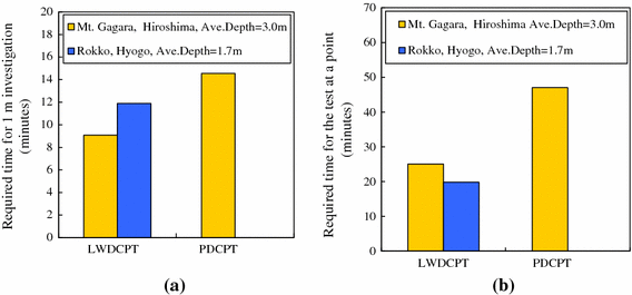
Time consumption to complete 1 m penetration

2.4 Correlations of cone resistance
The data collected from different sites were used for the development of correlations between the cone resistances. Athapaththu et al. (2007b) statistically analyzed the LWDCPT (q d ) and PDCPT (N d ) data collected from Mt. Gagara and developed a correlation between q d and N d for weathering remnants of decomposed granite as shown in Fig. 10a and Eq. (3). Here, N d is number of blow counts for 10-cm penetration and q d is in MPa. As far as authors aware of, there are no records available in the literature in correlating q d with N d for weathering remnants of decomposed granite. To develop a relationship between SPT N value and N d , data collected from Asakita, Saeki, Miyajima, and Kure were used. A fairly good linear relationship was established between N d and SPT N value by Athapaththu et al. (2007b) for the weathering remnants of decomposed granite and is shown in Fig. 10b and Eq. (4). Based on the above relationships, a cross-relationship between SPT N value and q d was developed and is shown in Eq. (5).

Relationship between cone resistance q d , N d , and N
2.5 Spatial variability of cone resistance
In general, soils have been formed by combination of various geological, environmental, and physiochemical processes. The in situ properties of soils vary with both vertically and horizontally are much important for most of the geotechnical analyses and designs. Several studies have investigated inherent uncertainty in natural soil properties (e.g., Kulhawy 1992; Lumb 1966; VanMarcke 1977, Vanmarcke 1983; Asaoka and A-Grivas 1982; Spry et al. 1988; Orchant et al. 1988; Soulie et al. 1990; Chaisson et al. 1995; Phoon and Kulhawy 1999). Soils derived from weathering remnants of decomposed granite are inherently heterogeneous. However, a little information is available on the spatial variability for weathering remnants of decomposed granite found in Japan (e.g., Galer 1999). Athapaththu et al. (2007b) carried out 2D kriging to analyze LWDCPT data collected at 5-, 2.5-, 1-, and 0.25-m grid spaces from Mt. Gagara to examine the variability in the space and also to determine the spacing for in situ tests for future investigations. The scatter of the cone resistance at different grid spaces was quantitatively analyzed by means of coefficient of variation (COV). COV measures the degree into which the set of data varies and often refers as the relative standard deviation. The mathematical formula to find COV is shown in Eq. (6).
where σ is the standard deviation and \(\overline{X}\) is the mean.
Figure 11a shows the range of COV along the soil profile (i.e., with depth) for different grid spaces, and Fig. 11b shows the COV varies with different grid spaces for selected depths, 0.1, 0.5, 1.0, 1.5, 2.0, and 2.5 m. The graphs reveal that the COV varies from 0 to 35 % for all range of cone resistance data collected at different grid spaces and depth. The COV of cone resistance can be presented about 20 % throughout the depths of weathering remnants of decomposed granite profiles at close proximity. This is almost similar in presenting typical geotechnical engineering parameters. More information about the analysis can be found from the literature furnished by authors (e.g., Athapaththu et al. 2007a).

COV varies with depth and different grid spaces. a COV varies with depth, b COV varies with grid spaces
Geo-statistics, and particularly the semi-variogram, has been shown to be a useful technique in predicting the data in recent studies, and hence, it has been applied for the present study. 2D kriging was adopted for the current analysis of cone resistance data. Semi-variograms for the Spherical and the Power Models were calculated for six different depths at Z = 0.1, 0.5, 1.0, 1.5, 2.0, and 2.5 m. The depth was measured from the ground surface, and the assumption was made as the soil profile is parallel to the bed rock.
The cone resistance, q d , at an unknown location of interest in XY plane with selected Z coordinate from the ‘n’ number of data can be written as in Eq. (7) below.
where q d (i*) is the cone resistance at unknown location, q d (i) is the measured cone resistance at the ith location, w i is an unknown weight for the measured value at the ith location and the summation of w i must be made equal to one to avoid biasness of the predictor.
The observed values and the predicted values of cone resistance are made as small as possible in order to minimize the statistical expectations of the following formula, from which the parameters of semi-variograms were obtained as shown in Eq. (8).
The measured semi-variance of ith and jth locations, \(\gamma ( {\text{h)}}_{\text{ij}}\), can be calculated from the basic formula shown in Eq. (9).
where q i d is the cone resistance at ith location, q j d is the cone resistance at jth location.
The solution to the minimization, constrained by un-biasedness, gives the kriging equations in a following matrix form
where γ ij denotes the modeled semi-variogram values between all pairs of observed q d values, γ ip denotes the modeled semi-variogram values based on the distance between the ith location and the prediction location, m (in the weight matrix) is an unknown constant, which arises because of the un-biasedness constraint and can be determined through the calculation process.
Solving the matrix as shown in Eq. (10), w i can be determined and the solution for unknown q d at location ‘p’ can be calculated from Eq. 7.
The cone resistance data collected from Mt. Gagara have been analyzed for six depth intervals (i.e., Z = 0.1, 0.5, 1.0, 1.5, 2.0, and 2.5 m) based on Eqs. (7), (8), (9), and (10). Figure 12 demonstrates the Spherical and the Power Models calculated for several depth intervals with their corresponding relationships. The Spherical Model was found to be the best-fitted semi-variogram for Masado profiles. The Power Model also showed reasonable agreement with the observed data. Therefore, these models can be applied to evaluate the cone resistance in an unknown location of interest. The range of influence of Masado soils was found to be varying with the profile depth. The correlated distance varies from 11 to 30 m with the depth increases from 0.1 to 2.5 m. This gives some idea for determination of grid spaces in carrying out in situ investigation of natural slopes having weathering remnants of decomposed granite.

Modeled semi-variograms for weathering remnants of decomposed granite profiles
3 Laboratory experimental setup and analysis
The main objective of this part of research was to establish sound relationship between shear strength parameters, ϕ d and c with cone resistance, q d , under different void ratios and degrees of saturation. To fulfill this task, a series of laboratory direct shear tests was carried out varying void ratios and degrees of saturation. Also, laboratory scale calibration tests were conducted based on LWDCPT for different void ratios and degrees of saturation. The methodology, data, analyses and results of these experiments are discussed in the following sections.
3.1 Direct shear tests on remolded samples
A series of laboratory experiments was carried out to develop relationships between shear strength parameters with void ratios and degrees of saturation. Soil samples collected at Mt. Gagara were fairly air-dried, and soils passing through 2-mm sieve were used for the laboratory tests. Reconstituted specimens were prepared for the laboratory direct shear tests. A sectional view of the direct shear apparatus used in this study is shown in Fig. 13.

Direct shear test apparatus with pore pressure measurements
Even though undisturbed specimens provide better representation of natural conditions than reconstituted specimens, it is practically difficult to make undisturbed specimens to a certain degree of saturation and void ratio. Therefore, reconstituted specimens were preferred for the laboratory tests to determine shear strength parameters under different void ratios and degrees of saturation. The testing program consisted of: (i) consolidated drained direct shear box tests conducted at void ratios ranging from 0.7 to 1.0 in 0.1 increments at a constant degree of saturation; (ii) repeat (i) at different degrees of saturation varying from 40 to 100 %. Also, tri-axial tests were conducted for different void ratios under 100 % degree of saturation. Direct shear tests with the measurement of pore pressure were conducted at all cases mentioned above except for the cases at the void ratio of 1.0. A ceramic disk with an air entry value 200 kPa was sealed on to the bottom half of the shear box. Pore pressure was measured through the pressure gauge connected to the ceramic disk as shown in Fig. 13.
The apparent cohesion, c d , and the friction angle, ϕ d , varying with void ratios under different degrees of saturation are shown in Fig. 14a and b, respectively. ϕ d is in degrees (°), c d is in kPa, and S r is in percentage (%). No clear trend was observed in ϕ d with degree of saturation, and data were scattered within a small range. Therefore, the average line was drawn to determine ϕ d varies with void ratios as shown in Fig. 14a. Further analyses of the data revealed that apparent cohesion ‘c d ’ can be developed as linear functions of void ratios for different degrees of saturation. It can be observed that the apparent cohesion decreases more than 50 % when the degree of saturation varies from 40 to 80 % in all range of void ratios. The graphical presentation can be deduced to the form of mathematical formula to express the shear strength parameters. Equation (11) shows the friction angle in terms of void ratios, while Eq. (12) displays the apparent cohesion in terms of void ratio and degree of saturation. Therefore, shear strength parameters can be calculated for known void ratio and degree of saturation for weathering remnants of decomposed granite based on the developed Eqs. (11) and (12).

Variation of apparent cohesion and friction angle with void ratios for different degrees of saturation. a Friction angle, b Apparent cohesion
3.2 Laboratory calibration tests
The main objective of this part of the research was to develop strength correlations between q d and shear strength parameters, c d and ϕ d , and thereby using the relationship to predict the shear strength parameters from the in situ LWDCPTs data. A series of LWDCPT was performed under void ratios ranging from 0.6 to 1.1 and degrees of saturation ranging from 50 to 90 %. Acryl cylinders each 29 cm in diameter and 20 cm in height were fastened through nuts and bolts, and porous plate was sealed to the bottom cylinder. The number of acryl cylinders used for each test was varied from two to six, and some tests were conducted by applying surcharge weights. Two to three trials of LWDCPTs were performed at each preparation, and specimens were taken at each cylinder for water content and void ratio measurements in order to compare the values before and after the tests. The slight variation of degrees of saturation and void ratios were observed along the soil chamber even though those parameters were fixed to a particular value prior to each test. However, those variations were considered in analyzing the test data. Comparatively, low values of cone resistance were recorded at high degrees of saturation. Moreover, high void ratios implicate low cone resistance. These are clearly displayed in the curves drawn in Fig. 15. The graphical relationships shown in Fig. 15 can be approximated to the formula shown in Eq. (13).
where q d5 was determined from the laboratory model tests conducted on surcharge weights. It is the cone resistance for 5 kPa overburden stress and can be found from Eq. (14). γ t is the overburden stress in kPa, and q d is in MPa.

Variation of cone resistance with void ratios under different degrees of saturation
By combining Eqs. (11), (12), and (13) Tsuchida et al. (2011) presented the shear strength parameters in terms of cone resistance as shown in Eqs. (15) and (16). Note that q d is in MPa, and S r is in %. The friction angle ϕ d is in degrees and cohesion (drained) in kPa. The developed formulas can be used to evaluate the shear strength parameters for a known degree of saturation.
3.3 Effect of fine content in determination of shear strength parameters
However, the effect of the fine content in shear strength parameters determined by cone resistance data has not been considered in above derivations. Therefore, this part of study was aimed to examine the variation of shear strength parameters, apparent cohesion, c d , and friction angle, ϕ d , with the different fine contents. Weathering remnants of decomposed granite collected from Mt. Gagara, same soil used for the laboratory tests to develop the relationship of shear strength parameters, sieved through 75-μm sieve. The soil passing through the sieve was used as the fine fraction. A series of laboratory direct shear tests was conducted varying fine fraction 0–15 % by weight. The degree of saturation and void ratio were kept to 40 % and 0.9, respectively, when preparing the remoulded samples. The fine fraction, void ratio and degree of saturation were determined after the tests even though those were made constant prior to the tests. Figure 16a and b shows the relationships between the friction angle and apparent cohesion vary with the fine content, respectively, obtained from the direct shear tests. Also, shear strength parameters estimated from Eqs. (11) and (12) were plotted in the same figure to compare variation. As seen in the figure, the friction angle determined from experiments is slightly greater than estimated values. The estimated value is 90 % of the experimental value irrespective of fine fraction, and therefore, estimated value needs to be corrected by multiplying 0.9. However, apparent cohesion was found to be increased with the fine fraction.

Variation of shear strength parameters with fine fraction based on direct shear test. a Friction angle, b Apparent cohesion
Figure 17a illustrates modification factor, the ratio of experimental value to the estimated value Eqs. (11) and (12) for the apparent cohesion. The modification factor increases with the fine content. The line was drawn considering the modification factor equal to 1 when there is no fine content in the soil. It can be applied to correct the apparent cohesion obtained in Eqs. (12) and (16). The apparent cohesion obtained from the experiments and that estimated from established equations before and after application of modification factor is shown in Fig. 17b. In determination of friction angle, a constant factor of 0.9 needs to be applied for the estimated values based on Eqs. (11) and (15).

Modification factor for the apparent cohesion and comparison
3.4 Comparison of estimated and experimental shear strength parameters for some field cases
As a whole, the friction angle can be determined from the proposed Eq. (15) for a known cone resistance data and known degree of saturation. However, when determining the apparent cohesion, the value calculated from Eq. (16) needs to be corrected based on Fig. 17. The proposed method to determine the shear strength parameters was examined through the triaxial tests conducted on undisturbed samples collected at 30 cm depth near the locations where LWDCPTs were carried out. The examination was carried out at 4 locations in Hiroshima Prefecture: Miyakegawa, Mukaihara, Yasu-ura, and Aratani valleys. The undisturbed samples were carefully trimmed into the triaxial specimen and compressed after the consolidation under confining stresses of 9.8, 19.6, and 39.2 kPa in drained conditions. The values of friction angle and the apparent cohesion were calculated from the data of tri-axial compression tests. The estimated shear strength parameters from the proposed equations based on cone resistance data and that determined through laboratory tests are illustrated in Fig. 18. It can be seen that the friction angle estimated and that obtained from tri-axil tests are slightly different in all sites. However, experimented and corrected apparent cohesion was found to be very close in Mukaihara and Yasuura valleys. More data need to make sound conclusion of the proposed modification factor.

Comparison of the experimental and estimated values of shear strength parameters
3.5 Application of the findings to geotechnical investigations and discussion
In this study, in situ investigation of natural slopes and shear strength parameters required for the analysis were thoroughly discussed. Further, shear strength parameters were evaluated based on the cone resistance data. The proposed method to evaluate shear strength parameters was successfully applied to number of slopes in Higashi Hiroshima city in Hiroshima Prefecture, Japan, for hazard assessment. A typical procedure for the investigation of a slope is summarized below.
-
1.
Gather the geological and topographical maps of the area of interest (susceptible valley of interest).
-
2.
The in situ testing points are determined at both sides of the valley center from top to the foot at 20-m intervals.
-
3.
At each testing point, the gradient of slope needs to be measured and the LWDCPTs are to be carried out. The soil samples will be taken at 30 cm depth for permeability tests, and other laboratory tests.
Figure 19 shows an example of investigation carried out at a valley in Mt. Gagara. Along the lines A and B, LWDCPTs and soil sampling were carried out. Based on the developed relationships, shear strength parameters were determined and are illustrated in the cross sections of lines A and B as drawn in Fig. 19b and c. In addition to that, two soil samples were taken for the permeability tests from the site. Using this information, it is possible to analyze the slope for the measured or predicted rainfall data. Tsuchida et al. (2014) carried out a case study for the failure occurred at Shiwa, in Hiroshima Prefecture, based on the proposed methodology and formulas and concluded that the shear strength parameters evaluated on proposed formulas well agreed to explain its failure. The rest of the slopes which is susceptible to failure can be well assed through the proposed methodology. However, collecting the information of individual slopes is challengeable as the number of susceptible slopes/valleys is very high in Hiroshima Prefecture. A day is required to investigate and carryout the in situ tests in a given site. Since the proposed formulas were developed for the weathering remnants of decomposed granite, more studies are needed to make the validity of the developed formulas to other soils and regions.

Pattern categorization of a slope in Mt. Gagara and cross sections with shear strength parameters
4 Conclusions
The overall objective of this research was to find an effective methodology to investigate the slopes susceptible to landslide disasters in Hiroshima Prefecture, Japan. Major concern was to find the shear strength parameters spatially to analyze the stability of slopes due to the shortcomings of the currently available methodologies. Some of such methods available in the literature are expensive and time-consuming or cannot be applicable for the steep slopes and slopes with difficult access. Authors are proposed new methodology based on recently developed LWDCPT. With the new method, it can be easily find the thickness of soil profile and other terrain conditions, spacing of in situ tests, and shear strength parameters required for the stability analyses. Based on the outcomes of this research, following conclusions are drawn.
-
1.
Six patterns of cone resistance varying along the depth were identified in the profiles having weathering remnants of decomposed granite. The proposed six patterns were successfully applied for the different locations and found that most of the soundings can be fitted into one of the pattern. Therefore, proposed classification can be successfully applied to the terrains having weathering remnants of decomposed granite.
-
2.
It was found that the use of newly developed LWDCPT is convenient due to its automatic recording to a greater accuracy of penetration resistance, simplicity in handling, and less time in completing a typical site characterization. Therefore, it has been proposed for carrying out the site investigations in the slopes and valleys in Hiroshima Prefecture, Japan. LWDCPT can be applied to other soils and different regions for site characterization purposes and to obtain the shear strength parameters. However, this needs extensive testing program as done for weathered remnants of decomposed granite under this study.
-
3.
A good correlation (q d = ½N 3/4 d ) was established between the data collected from LWDCPT and PDCPT. LWDCPT provides more reliable accurate results than PDCPT. Also, LWDCPT was found to be more efficient than PDCPT in completing a typical site characterization. Linear relationship was identified between SPT N value and N d as, N d = 2.2 N. Based on these relationships, an approximate cross-relation was identified between q d with SPT N value as N = 1.15q 4/3 d . The use of these equations for other soils than for decomposed granites needs to be examined.
-
4.
The scatter of the cone resistance at different grid spaces was quantitatively analyzed by means of coefficient of variation (COV) and was found that COV varies 0–35 % for all range of data. The Spherical Model was found to be the best-fitted semi-variogram for the decomposed granitic profiles, and hence, it can be applied to evaluate the cone resistance at unknown location. The correlated distance varies from 11 m to 30 m with the depth increases from 0.1 to 2.5 m, respectively. This gives some idea for determination of grid spaces in carrying out in situ investigation of natural slopes of weathering remnants of decomposed granite.
-
5.
The friction angle of reconstituted soils of weathering remnants of decomposed granite was found to be linearly varied with the void ratios approximately. Fairly good linearly varying relationships were established between void ratios and apparent cohesion under different degrees of saturation. The equations are:
$$\phi_{d} = 52.7 - 19.2e$$$$c_{d} = 27.5 - 0.146S_{r} - 14.2e$$ -
6.
Based on the cone resistance data, q d , relationships were developed to calculate shear strength parameters in terms of degrees of saturation as:
$$\phi_{d} = 29.9 + 1.61\ln (q_{d5} ) + 0.142S{}_{r}$$$$c_{d} = 10.6 + 1.19\ln (q_{d5} ) - 0.041S_{r}$$
The proposed formulas can be successfully applied to determine the shear strength parameters for known degree of saturation. Knowing the fine content of the soils, better estimation can be made for friction angle and apparent cohesion based on the modification factors proposed in this study.
References
Asaoka A, A-Grivas D (1982) Spatial variability of the undrained strength of clays. J Geotech Eng 108(GT5). ASCE, New York, pp 743–756
Athapaththu AMRG, Tsuchida T, Sato T, Suga K (2005) A lightweight dynamic cone penetrometer for the investigation of natural Masado slopes. In 4th International conference on civil and environment engineering. Hiroshima University, pp 279–284
Athapaththu AMRG, Tsuchida T, Sato T, Suga K (2006) Evaluation of in situ shear strength of natural Masado slopes. Geotechnical division–ISOPE 2006, San Francisco, International offshore and polar engineering, vol 2, pp 324–331
Athapaththu AMRG, Tsuchida T, Suga K, Sato T (2006) Investigation of spatial variability of natural Masado slopes. In: 5th International conference on civil and environment engineering. Hiroshima University, pp 67–78
Athapaththu AMRG, Tsuchida T, Suga K, Kano S (2007a) A lightweight dynamic cone penetrometer for evaluation of natural Masado slopes. J Jpn Soc Civil Eng JSCE 63(2):403–416
Athapaththu AMRG, Tsuchida T, Suga K, Nakai S, Takeuchi J (2007b) Evaluation of in situ strength variability of masado soils. J Jpn Soc Civil Eng JSCE 63(3):848–861
Cassan M (1988) Les essays in situ en mechanique des sols, realization et interpretation. Eyrolles 1, Paris, 2nd ed., pp 146–151
Chaigneau L, Gourves R, Boissier D (2000) compaction control with a dynamic cone penetrometer. Proceedings of international workshop on compaction of soils, Granulates and powders, Innsbruck, pp 103–109
Chaisson P, Lafleur J, Soulie M, Law KT (1995) Characterizing spatial variability of a clay by geostatistics. Can Geot J 32:1–10
Dissanayake AK (2002) A study on the initiation of rain induced landslides in decomposed granite slopes. PhD thesis. Hiroshima University. Japan, pp 8–13
Futagami T, Sakai H, Kakugawa K, Fujimoto A, Fukuhara T, Fujiwara Y, Sakurai S (2010) Debris flows promoted by mechanical deterioration of the ground due to eutrophication of hillside ecosystems; risk analysis VII, WIT transactions on information and communication technologies vol 43, pp 703–714
Galer MM (1999) A study on the mechanical properties of undisturbed decomposed granite based on testing and triaxial testing results under elevated confining pressure. PhD thesis. Hiroshima University. Japan, pp 1–34
Hiroshima Prefecture: http://www.pref.hiroshima.lg.jp/page/1171592994610/index.html
Ito Y, Iwasaki T, Nobumoto M, Miyata Y, Murata Y (2006) The application case of a new portable dynamic probing test. In: Symposium on application of recent geotechnical investigations and testing methods, pp 23–26
Japanese standards and explanations of geotechnical and geoenvironmental investigation methods (2013), The Japan geotech. Society, 1 edn, pp 208–209 (in Japanese)
Kulhawy FH (1992) On evaluation of static soil properties: Instability and performances of slopes and embankments II (GSP 31). ASCE, New York, pp 95–115
Langton DD (1999) The PANDA-lightweight penetrometer for soil investigation and monitoring material compaction. Ground Eng, pp 33–37
Lumb P (1966) The variability of natural soils. Can Geot J 3(2):74–97
Nakai S, Sasaki Y, Kaibori M, Moriwaki T (2006) Rainfall index for warning and evacuation against sediment related disaster: reexamination of rainfall index Rf, and proposal of R’. Soils Found 46(4):465–475
Orchant CJ, Kulhawy FH, Trautmann CH (1988) Reliability based foundation design for transmission line structures: critical evaluation of in situ test methods. Electric power research institute. Palo Alto, California. Report EL-5507(2)
Phoon KK, Kulhawy FH (1999) Characterization of geotechnical variability. Can Geot J 36:625–639
Sasaki Y, Moriwaki T, Kano S, Shiraishi Y (2001) Characteristics of precipitation induced slope failure disaster in Hiroshima prefecture of June 29, 1999 and rainfall index for warning against slope failure disaster. Soils Found 49:16–18
Soulie M, Montes P, Silvestri V (1990) Modelling of spatial variability of soil parameters. Can Geot J 27:617–630
Spry MJ, Kulhawy FH, Grigoriu MD (1988) Reliability based foundation design for transmission line structures: geotechnical site characterization strategy. Electric power research institute. Palo Alto, California. Report EL-5507(1)
Statistical Handbook of Japan 2013, Statistics Bureau, Ministry of Internal Affairs and Communications, (web site-http://www.stat.go.jp/english/data/handbook/c0117.htm )
Tsuchida T, Athapaththu AMRG, Kano S, Suga K (2011) Estimation of in situ shear strength parameters of weathered granitic (Masado) slopes using lightweight dynamic cone penetrometer. Soils Found 51(3):497–512
Tsuchida T, Kano S, Nakagawa S, Kaibori M, Nakai N, Kitayama N (2014) Landslide and mudflow disaster in disposal site of surplus soil at Higashi-Hiroshima due to heavy rainfall in 2009. Soil Found 54(4): (accepted for publication)
Vanmarcke EH (1977) Probabilistic modeling of soil profiles. J Geotech Eng 103(GT11). ASCE, New York, pp 1227–1246
Vanmarcke EH (1983) Random fields: analysis and synthesis. MIT Press, Cambridge
Wang G, Kyoji S, Fukuoka H (2003) Downslope volume enlargement of a debris slide-debris flow in the 1999 Hiroshima, Japan rainstorm 2003. Eng Geol 69(3–4):309–330
Author information
Authors and Affiliations
Corresponding author
Rights and permissions
Open Access This article is distributed under the terms of the Creative Commons Attribution License which permits any use, distribution, and reproduction in any medium, provided the original author(s) and the source are credited.
About this article

Cite this article
Athapaththu, A.M.R.G., Tsuchida, T. & Kano, S. A new geotechnical method for natural slope exploration and analysis. Nat Hazards 75, 1327–1348 (2015). https://doi.org/10.1007/s11069-014-1384-0
Received:
Accepted:
Published:
Issue Date:
DOI: https://doi.org/10.1007/s11069-014-1384-0