Optimizing wheel profiles and suspensions for railway vehicles operating on specific lines to reduce wheel wear: a case study

Abstract

The selection of a wheel profile is a topic of great interest as it can affect running performances and wheel wear, which needs to be determined based on the actual operational line. Most existing studies, however, aim to improve running performances or reduce contact forces/wear/rolling contact fatigue (RCF) on curves with ideal radii, with little attention to the track layout parameters, including curves, superelevation, gauge, and cant, etc. In contrast, with the expansion of urbanization, as well as some unique geographic or economic reasons, more and more railway vehicles shuttle on fixed lines. For these vehicles, the traditional wheel profile designing method may not be the optimal choice. In this sense, this paper presents a novel wheel profile designing method, which combines FaSrtip, wheel material loss function developed by University of Sheffield (USFD function), and Kriging surrogate model (KSM), to reduce wheel wear for these vehicles that primarily operate on fixed lines, for which an Sgnss wagon running on the German Blankenburg–Rübeland railway line is introduced as a case. Besides, regarding the influence of vehicle suspension characteristics on wheel wear, most of the studies have studied the lateral stiffness, longitudinal stiffness, and yaw damper characteristics of suspension systems, since these parameters have an obvious influence on wheel wear. However, there is currently little research on the relationship between the vertical suspension characteristics and wheel wear. Therefore, it is also investigated in this paper, and a suggestion for the arrangement of the vertical primary spring stiffness of the Y25 bogie is given.

1 Introduction

The increase in railway vehicle speed, axle load, and traffic volume exacerbates wheel wear, resulting in shorter wheel re-profiling mileage. At present, wheel wear has become one of the most critical issues affecting the operating cost and vehicle-track performance [1, 2]. Reducing wheel wear, therefore, is a topic of big interest.

A lot of studies have shown that a reasonable wheel–rail (WR) matching form can directly and effectively reduce wheel wear [3]. As shown in Fig. 1, the WR contact region can be divided into three regions [2]: (1) Region A: wheel tread–rail head. The WR contact is typically located in this region and usually occurs when the vehicle is running on straight tracks or curves with large radii. Lowest contact pressures and lateral forces occur in this region, which results in lower wear between the wheel tread and the rail head; (2) Region B: wheel flange–rail gauge corner. The WR contact tends to occur in this region when the vehicle is running on curves with small radii. The contact patch is much smaller than that in region A. This region yields higher contact pressures and sliding velocities, resulting in severe wear between the wheel flange and the rail gauge corner; (3) Region C: contact between field sides of wheel and rail. Contact is least likely to appear in this region. The occurrence of the contact in this region will result in incorrect steering of the wheelset and severe wheel wear. Therefore, letting the WR contact occur primarily in Region A is the optimal solution to reduce wheel wear, in which a reasonable wheel profile plays a key role.

Fig. 1

WR contact regions

Besides, some studies have shown that the characteristics of vehicle suspensions could also affect wheel wear to some extent [4,5,6,7]. We believe that unreasonable suspension parameters may lead to two mechanisms that increase WR wear: (1) It may affect the WR creepages and sliding velocities, thereby affecting wheel wear; (2) It may also cause WR contact to occur frequently in Region B described in Fig. 1, resulting in severe wear between the wheel flange and the rail gauge corner.

Based on the above considerations, this work aims to reduce wheel wear by optimizing the wheel profile and the vehicle suspension system.

1.1 Existing methods

1.1.1 Wheel profile optimization methods

A suitable wheel profile can reduce wheel wear and improve running performance. The optimization of wheel profiles, therefore, has been a meaningful topic since the dawn of railway vehicles. The approaches with different strategies for the development of a new, theoretical wheel profile over the past two decades can be mainly classified into three categories [8, 9]: (1) bio-inspired optimization algorithm; (2) target-based technique; and (3) direct evaluation (wear model).

Bio-inspired optimization algorithm

The most common bio-inspired algorithm used to optimize wheel wear is the genetic algorithm (GA) [10]. In terms of the single-objective optimization of wheel profiles, Santamaria et al. [11] designed an optimal wheel profile using GA, in which the rolling radius difference function (RRD) was considered as the optimization object. Dynamic simulation results showed that the optimized wheel profile calculated by this method could obtain a lower wear rate and higher running performance. In terms of the multi-objective optimization of wheel profiles, Persson and Iwnicki [12] applied GA to reflect the influence of different profiles on various factors including wear, contact stress, track shift force, derailment quotient, and passenger comfort. Choi et al. [13] applied GA to minimize the flange wear and surface fatigue of a wheel, in which the boundary conditions were given, such as derailment coefficient, lateral WR force, the possibility of overturning and vertical load. Novales et al. [14] used GA to select the optimal wheel profile to balance the derailment coefficient, wear and WR contact stress. Firlik et al. [8] designed a wheel profile using GA for optimizing the wear index, derailment coefficient, and contact area. Another classical bio-inspired algorithm that has been used in wheel profile optimization is the particle swarm optimization algorithm (PSO) [15]. For instance, based on the Non-Uniform Rational B-Spline (NURBS) curve theory, Lin et al. [16] used PSO to design an LM thin flange wheel profile, in which the mean values of wear work and lateral force of wheelset were considered as objective functions, and the profile curve concavity and continuity were set as geometric constraints. The result showed that the average wear work of the first wheelset was reduced by 55.97% compared with the standard LM profile. Cui et al. [17] used PSO to design a new wheel profile for the CRH1 train in China, in which a weighted factor that considered ride comfort and wheel wear was introduced as the objective function, and the derailment-related indexes were considered as the constraints. The result showed that the new wheel profile designed by PSO could significantly reduce the wheel flange/rail gauge corner wear on the premise of ensuring the dynamic behavior of the vehicle.

Target-based technique

Currently, there are four main kinds of target-based techniques: target RRD, target conicity, target contact angle, and target WR normal gap. Based on the target RRD, Shevtsov et al. [18] proposed a numerical optimization technique to optimize the wheel profile, in which the RRD function was used to characterize the superiority of different wheel profiles and was set as the optimization object. The results showed that a reasonable increase in RRD could improve the curve negotiation ability and decrease the wear rate. In [19], considering both RCF and wear, Shevtsov et al. achieved an optimized wheel profile. The results of the dynamic simulations showed that the use of the optimized profile resulted in a small increase in wear index and a small decrease in surface fatigue. This technique was also studied in [11, 20,21,22]. Similar techniques were presented in [9, 23], i.e., target conicity [9] and target contact angle [23], respectively. Concerning the target WR normal gap, Cui et al. [24] thought that a small weighted WR normal gap could make a conformal contact, thereby reducing the contact stress and decreasing the wear and RCF.

Direct evaluation (wear model)

This approach is used to reduce wheel wear and can visually present the result. Ignesti et al. [25] used FASTSIM and USFD wear function to calculate the material loss under different wheel profiles. In their study, four different kinds of wheel profiles, CD1, DR1, DR2, and S1002, were investigated. The wear evolution of these profiles could be visually presented to help people select the optimal wheel profile. Similar studies were presented in [26, 27].

When designing a wheel profile, several of the listed strategies can be used simultaneously.

1.1.2 Vehicle suspension optimization concerning wheel wear

From the perspective of wheel wear, Fergusson et al. [4] investigated the longitudinal and lateral primary suspension stiffness and the centre plate friction of a self-steering three-piece bogie. A large number of simulation results showed that these three parameters had a great influence on the wear number and dynamics performances including derailment coefficient, angle of attack, WR creepage, etc., in which three curves of different radii (300, 500, and 1000 m) were discussed. Through observation, an optimized combination of these three parameters was found, and it showed that a reasonable combination of these three parameters could reduce the wear number by up to 50%. Mazzola et al. [5] studied the influence of the wheelbase and suspension system on the running safety and wear of a non-powered high-speed car. In their work, the longitudinal and lateral stiffnesses of the primary suspension and the yaw damper coefficient of the secondary system were investigated. The results showed that different combinations of these three parameters had a different influence on the wear index. Finally, the optimal combination was calculated by polynomial interpolation functions. Bideleh et al. [6] explored the influence of the arrangement of the suspension system on ride comfort and wear number. In their work, GA was integrated into MATLAB/SIMPACK co-simulation to optimize the bogie suspension system, in which the ride comfort and wear were considered as objective functions, and the track shift force, stability, and risk of the derailment were set as constraints. The optimization results showed that the asymmetric suspension system revealed remarkable benefits in wear reduction when the vehicle operated on tracks with small radii. In [7] Bideleh investigated the effects of primary and secondary suspension stiffness and damping components on the wheel wear of a railway vehicle model with 50 degrees of freedom (DOFs) based on the multiplicative dimensional reduction method (M-DRM). It was found that the wear was most sensitive to the longitudinal and lateral primary springs. However, for the symmetric vehicle model, as the radius of curvature of the track increased, the effects of the longitudinal and vertical secondary springs became dominant. In the case of large curves and straight tracks, yaw dampers could also significantly affect wear. It was further stated that the sensitivity analysis results obtained in this paper could narrow down the number of the input design parameters for optimization problems of bogie suspension components and improve the computational efficiency. Ashtiani [28] studied the dynamic characteristics of the friction wedge geometry in the secondary suspension of a freight wagon with three-piece bogies. An optimization formulation was proposed to improve the performance of the wagon in terms of minimizing the extreme normal WR contact and vertical carbody acceleration. The optimal wedge geometry is then evaluated in terms of critical hunting speed and curving performance of wagon. The beveled geometry of the wedge with optimal angles presents an improvement in higher critical hunting speed and lower derailment coefficient. Although the relationship between the wedge geometry and wheel wear was not directly discussed in this article, it showed that the wedge geometry could affect the WR force, thus indicating that the wedge geometry may also have an effect on wheel wear. A similar study was presented in [29].

1.2 Motivation

Indeed, the aforementioned methods in Sect. 1.1.1 have great potential for wheel profile optimization if the models are accurately established and the strategies are correctly formulated. Most of these studies, however, have aimed at improving the running performance and/or reducing contact force/wear/RCF on small-section curves with ideal radii, losing the big picture of whole route [30]. However, the whole route usually consists of a lot of sections with different track layout parameters, such as superelevation, gauge, cant, and arc. Furthermore, some studies have shown that the track layout parameters have a significant influence on wheel wear. For example, Pombo et al. [31] investigated the influence of rail cant on wheel wear growth, in which the wheel profile S1002 and the rail profile UIC60 were used. The results revealed that the reprofiling intervals obtained when running on the track with a rail cant of 1/40 were larger than when traveling on a track with a rail cant of 1/20. Gao et al. [32] studied the superelevation setting for a 400-meter-radius curve of the China Shen-shuo railway line based on Hertzian theory and FASTSIM algorithm. The simulation results showed that the superelevation had a great influence on wheel wear. Therefore, it is necessary to consider the actual track layout parameters of the whole route when developing wheel profiles.

More importantly, with the expansion of urbanization, more and more railway vehicles shuttle on special lines, such as metro, light rail, and tram. In addition, due to some unique geographic or economic reasons, some vehicles typically operate on a designated line. For example, some CRH1A and CRH380A trains only run on the China Hainan Roundabout railway line because of the unique island geography of Hainan province. Some CRH380A trains mainly run on China Shanghai–Hangzhou special passenger line because of the heavy transportation tasks [33]. Furthermore, some vehicles that undertake special tasks often run on fixed lines, such as those coal wagons on the China Datong–Qinhuangdao railway line [34], the WLE beer wagons on German Warstein–München Riem railway line [35], and the lime wagons running on German Blankenburg–Rübeland railway line introduced in this paper [36]. For the aforementioned vehicles running on fixed lines, the traditional wheel profile or the profile designed by the approaches described in Sect. 1.1.1 may not be the optimal choice. In this sense, a novel wheel profile designing method, which considers the actual track layout parameters, for reducing wheel wear for these vehicles operating on fixes lines is introduced in this paper.

Regarding the influence of suspension optimization on wheel wear, the existing researches described in Sect. 1.1.2 have studied the lateral stiffness, longitudinal stiffness, and yaw damper characteristics of suspension systems, since these parameters have an obvious influence on wheel wear. However, as far as the authors know, there is currently little research on the relationship between the vertical suspension characteristics and wheel wear. Therefore, it is also investigated in this paper.

1.3 Proposed method

The basic idea of this paper is first to calculate the wheel wear under different initial wheel profiles and different vertical spring characteristics of the primary suspension of the Y25 bogie by the wear model and then establish the response model between these three parameters through the KSM. Finally, the optimal wheel profile is found and the relationship between vertical spring characteristics of the primary suspension and wheel wear is investigated based on KSM technique.

1.3.1 A FaStrip-USFD based wheel wear model

The wheel wear calculation model is made up of two submodels: WR local contact model and wheel material loss model [37, 38].

The WR local contact model consists of a WR normal contact model and a WR tangential contact model [39]. In our work, the Hertzian contact model [40] is applied as the WR normal contact model since it can balance the calculation efficiency and accuracy [41]. Concerning the WR tangential contact model, it includes Shen–Hedrick–Elkins (S.H.E) [42], Polach [43], FASTSIM [44], etc. Among them, The S.H.E theory and the Polach method cannot obtain the shear stress distribution and sliding velocity of the contact patch, which are not suitable for wheel wear calculation. The FASTSIM cannot ideally solve the shear stress distribution and stick–slip division issues, which may cause significant errors in wear prediction [45]. Recently, a novel WR local contact model, FaStrip [45], has been proposed. This method is based on Strip theory, Kalker linear theory, and FASTSIM, and can obtain high accuracy on both shear stresses and relative slip velocities. Therefore, it is applied in this paper.

Concerning the wheel material loss model, it can be mainly classified into the following two categories [46,47,48]:

• Archard model [49, 50], where the material loss ($V_{w}$) is proportional to the normal force ($N$) and the sliding distance ($S$) divided by the material hardness ($H$), i.e., $V_{w} = {kNS} / {H}$.

• $T - \gamma$ [51], which assumes that the material loss ($T\gamma$) is proportional to the frictional energy dissipated in the contact patch. It is expressed as the sum of the products of creep forces and creepages for the lateral, longitudinal, and spin components, i.e., $T\gamma = T_{x} \gamma _{x} + T_{y} \gamma _{y} + M_{z} \omega _{z}$. USFD function [52], as a kind of $T \mbox{--} \gamma$ method, is applied in this paper.

In this work, the FaStrip algorithm and USFD function are combined to calculate the wheel material loss. This method is called as FaStrip-USFD.

1.3.2 KSM

Simulations involving parametric studies are often based on repetitive modeling, which greatly increases the calculation amount. For example, in the case of the vehicle multibody dynamics simulation (MBS) model built in this research, running the simulation takes more than 600 CPU hours. The calculation amount of such simulations is so large that the railway industry is reluctant to do many deterministic analyses. In addition, the test process involves steps such as numerical calculation, analysis, etc., involving a large number of uncertainties. It not only consumes much human labor but also may increase errors [53]. Therefore, it is of interest to find a high-efficiency and reliable method to simplify the simulation procedure.

Recently, the KSM technique [54] has begun to be used in railway engineering[55], since it can overcome the above two shortages. This technique uses a small number of sample points that fit a specific sampling strategy to construct a simplified mathematical model that approximates the original complex model. Therefore, it can replace the original analytical model and simplify the calculation process while maintaining high calculation accuracy. In our work, this technique [56] is introduced to build the relationship between the wear area, wheel profile adjustment factor and vertical outer primary stiffness, since it is an unbiased estimation model that fully considers the spatial correlation of variables.

1.4 Contribution and structure of this paper

The main work of this paper is summarized as follows:

• (1) For those vehicles that mainly operate on fixed lines, a FaStrip-USFD-KSM based model for optimizing the wheel profile and vehicle suspension to reduce wheel wear is proposed, where the German Blankenburg–Rübeland railway line with detailed track layout parameters and an Sgnss wagon are established.

• (2) Based on the S1002 profile, an adjustment factor is proposed to optimize the wheel profile. This method simplifies complex curve design problems by using classical transition curves.

• (3) The influence of the vertical primary suspension characteristics on wheel wear is studied, and a suggestion for the arrangement of the vertical primary spring stiffnesses of the Y25 bogie is given.

The rest of this paper is structured as follows. In Sect. 2 the German Blankenburg–Rübeland railway line and an Sgnss wagon are modeled, where the detailed track layout parameters are considered. In Sect. 3 the theories of the FaStrip, USFD wear function, and KSM are briefly described, and a FaStrip-USFD-KSM based optimization method for reducing wheel wear is proposed. In Sect. 4 a case study of the Sgnss wagon running on the Rübeland–Blankenburg line is presented. In Sect. 5 quasi-static and dynamic tests for acceptance of the optimized wheel profile according to the standard EN 14363 are presented. Discussion and conclusions are briefly drawn in Sect. 6.

2 Operational line and vehicle model

2.1 Operational line

The railway line introduced in this work is the Blankenburg–Rübeland line located in Germany. This route was built starting in about 1880 in Blankenberge in the Harz Mountains, connecting the companies located there to the railway network, such as Hüttenwerke, Kalkbranntwerke, etc. On the one hand, bulk goods must be transported away. On the other hand, raw materials such as coal and lime are supplied [36, 57]. Currently, most of the vehicles on this route mainly serve the lime project of the Fels-Werke GmbH in Harz. The corresponding transport route starts in Blankenberge and leads to Michaelstein. Then the wagon continues to Rübeland. The return trips are carried out in the opposite order, forming a cycle of the Rübelandbahn with a total length of 31.46 km [36]. The route is shown in Fig. 2. It can be seen that the route contains many tight curves which may result in severe wheel wear of vehicles running on this line. In our work, we aim to optimize the wheel profile to reduce wheel wear and further reduce operating costs.

Fig. 2

Rübeland–Blänkenburg railway line

The experiment data (radius, superelevation, rail cant, gauge distance, vehicle speed) used in this paper were supported by the DynoTRAIN project, which was funded by the European Commission. This project started on June 1, 2009, and ended on September 30, 2013. The authors’ group, Fachgebiet Schienenfahrzeuge, TU Berlin, was one of the partners in this project. More information about this project can be found in [58].

The curvature, superelevation, and cant concerning the route were provided by the existing route plan [59, 60]. Figure 3(a) shows the reciprocal of the radius of the arc, which clearly shows that the line contains many tight curves, and some sections even have a radius of less than 200 m. These small radii result in high contact forces and sliding velocities, greatly increasing the wear amount. It is necessary to optimize the wheel profiles of those vehicles that primarily operate on this line. Figure 3(b) shows the superelevation. The standard cant used in Germany usually is 1:40 (i.e., 0.025). This value, however, is not constant on the Blankenburg–Rübeland line. The increment of cant is shown in Fig. 3(c), where the negative sign represents the increase in slope.

Fig. 3

Track layout parameters of the route (a-d) and vehicle speed (e) (Color figure online.)

There is no direct information available for the gauge. This value, however, has a significant influence on wheel wear [61], especially for the contact point position on the wheel. Different track gauge results in a different wear pattern, which means that the gauge value is a necessary input variable for the simulation scenario. A change occurs mainly in arcs and is referred to as a gauge increment, as usually positive changes occur. In our work, the approach, that the value is proportional to the arc curvature, is used. It is assumed that there is a gauge increment of 0.02 m at $r_{\mathrm{arc}} = 100~\mbox{m}$ (Eq. (1)) and the standard track gauge (1.435 m) is installed in the straight line.

$$ \Delta S_{w} = \frac{100~\text{m}}{r_{\mathrm{arc}}} \cdot 0.02~\text{m}. $$

(1)

Finally, the gauge increment is shown in Fig. 3(d). The vehicle speed was measured by the authors’ technique team [60], a total of four tracking tests were performed. To facilitate the simulation, the authors corrected these speed curves. The final results are shown in Fig. 3(e).

There are two points should be noted here:

• (1) Lubricants significantly affect the wheel wear [62], in our work it is not considered since the freight wagon we used was not equipped with the lubrication device, and the WR friction coefficient used in the whole simulation is 0.35.

• (2) In the subsequent wheel wear calculation, the used vehicle speed is corrected based on the actual test speed (Fig. 3(e)), which simply considers the influence of the train’s traction and braking on wheel wear, rather than a comprehensive consideration. This will affect the calculation accuracy to some extent, but fortunately, the braking and traction distance is not long relative to the total mileage.

More information concerning the speed can be found in [36, 60].

2.2 Vehicle model

The vehicle model introduced here is an Sgnss wagon, which is modeled in SIMPCAK 2020.2. The MBS model is made up of one car body, two bogie frames, four wheelsets, and eight axleboxes. It has 55 DOFs in total. Since one of the purposes of our work is to study the effects of vertical suspension characteristics on wheel wear, it is important to accurately establish the suspension system.

The primary suspension (Fig. 4(a)) is between the bogie frame and the axlebox. Each suspension has two spring sets, and each spring set has two nested coil springs, i.e., an inner coil spring and an outer coil spring. The outer spring acts independently of the empty load. The inner spring ($l_{r}= 0.234~\mbox{m}$) is shorter than the outer one ($l_{r}= 0.26~\mbox{m}$) so that it acts only from a certain vertical load. The detailed information about the spring set is shown in Table 1. As steel springs, the coil spring has minimal internal damping and its damping, therefore, is ignored. The frictional damping is mainly provided by an inclined Lenoir link, which connects the bogie frame and the spring holder. Based on this, the primary suspension is modeled as follows. The vertical stiffness for each spring set is modelled as a force element (Fig. 5(a)), which is a combination of the inner spring and outer spring stiffnesses listed in Table 1. The longitudinal stiffness per axle stems from the pendulum stiffness of the Lenoir link and the horizontal stiffness of the nested spring, it is realised by feeding a formula in the force element. The relationship between the longitudinal stiffness and vertical displacement is shown in (Fig. 5(b)). The lateral stiffness is a step function of the vertical deflection of the outer spring due to the load-depending-effect of the inner springs. The relationship between the lateral stiffness and vertical displacement is shown in Fig. 5(c). The bump stops of the spring sets are also considered in the longitudinal and vertical directions. The lateral and vertical friction is modelled as dry Coulomb friction, where the friction force is proportional to the normal load. More description can be found in [63].

Fig. 4

The primary suspension (a) and unsprung side bearer (b)

Fig. 5

Characteristics for the primary vertical force (a), primary longitudinal stiffness (b), primary lateral stiffness (c), side bearer’s vertical force (d), side bearer’s longitudinal force (e), and side bearer’s lateral force (f)

Table 1 Date of primary suspension

There is no real secondary suspension on the Y25 bogie. The secondary suspension system consists of a spherical center pivot, only allowing three rotational DOFs, and two side bearers (Fig. 4(b)). The center pivot is modeled using a constraint element for preventing translational motions between wagon body and bogie frame as well as four frictional force elements. The side bearers are mounted outboard of the bogie pivot, providing friction damping in yaw and restraint in roll. They each consist of horizontal friction plates mounted on twin vertical coil springs. Each side bearer is modeled as a mass element and two force elements. One connects the bogie frame and the mass element, and has the summed stiffness of the two coil springs, taking into account the bump stop, where the characteristics of the vertical, longitudinal and lateral forces are shown in Figs. 5(d), (e), and (f), respectively. The other one represents the frictional force between the wagon body and the side bearer, whose normal force stems from a constraint element between the wagon body and the mass element. Moreover, the accuracy of these parameters was verified by using the actual test data [53, 64].

In order to make the simulation results closer to reality, the track irregularities are also considered. In this model, the PSD of the typical European spectrum (ERRI B176) defined in SIMPACK is applied as the track irregularities. The track is modeled using a discrete model including a tie with three DOFs (lateral, vertical and roll) placed under each wheelset. More information concerning the MBS model, including the modeling steps and the detailed parameters, can be found in the authors’ previous work [65, 66].

Finally, the simulated route (Fig. 6(a)) and the MBS model of the vehicle (Fig. 6(b)) are shown in Fig. 6. By comparing Fig. 6(a) with Fig. 2, it can be seen that the simulated line and the actual line are almost identical. The data of interest are shown in Table 2. One thing may be of interest to authors is that in the current version of SIMPACK, rail cant cannot be directly defined as a continuously changing value like the radius and superelevation. This step can be achieved by the EXCITATION ROLL function under RAIL-RELATED of TRACKS. This simple strategy can avoid complex secondary development.

Fig. 6

Simulated Rübeland–Blänkenburg railway line (a) and MBS model (b) of the Sgnss wagon

Table 2 Primary parameters of the lime wagon

3 FaStrip-USFD-KSM based optimization method

3.1 Theories of methods

3.1.1 FaStrip-USFD

Currently, the most common wheel profile calculation method is based on the WR local contact model and wheel material loss model [67,68,69,70,71,72,73], in which, the WR local contact model consists of a WR normal contact model and a WR tangential contact model. The WR normal contact model originated from the Hertzian contact theory, i.e., Hertzian contact model, which is currently the most widely used in the WR normal contact analysis [74]. However, in the actual operation of the train, the WR contact may be a conformal contact and/or a non-Hertzian contact. The approaches for solving conformal WR contact problems include the finite element (FEM) method [75, 76], the CONTACT’s boundary element approach together with the numerical influence coefficients [77], a computer program called WEAR [78], etc. The approaches for solving non-Hertzian WR contact problems include the FEM, Kalker’s variational method [79], Linder method [80], Kik–Piotrowski (KP) model [81], Extended Kik–Piotrowski (EKP) model [82], Modified Kik–Piotrowski (MKP) model [83], Ayasse–Chollet model (STRIPES) [84], ANALYN [85], etc. These listed methods are generally more suitable for describing WR contacts than Hertzian contact model. However, these methods have a much higher computational effort than Hertzian contacts. Besides, in [41], three non-Hertzian contact models, namely KPM, STRIPES, and ANALYN, were compared to Hertzian contact model and the CONTACT code in terms of the normal contact solution, and the tangential contact solutions and wheel wear material loss were calculated by FASTSIM and USFD wear function, respectively. The results indicated that using Hertzian contact model to solve the WR normal contact problem in wheel wear simulation was a good choice from a compromise between the calculation efficiency and accuracy. Hertzian contact model, therefore, is applied to solve the WR normal contact in our work. More information on non-Hertzian contact models can be found in [86, 87] or the author’s previous work [83].

Concerning the WR tangential contact model, classical WR tangential contact models include S.H.E. [42], Polach [43], FASTSIM [44], etc. Among them, the S.H.E. theory and the Polach method cannot obtain the shear stress distribution and sliding velocity of the contact patch, which are not suitable for the wheel wear calculation. FASTSIM, currently, is the most widely used. In this theory, the shear stress in the stick area is assumed to increase linearly from the leading edge until the traction bound is reached. The traction bound is assumed as the product of the contact pressure and the friction coefficient. Although FASTSIM utilizes the Hertzian solution for normal contact solution, which yields an elliptical pressure distribution, the traction bound in FASTSIM is taken to be parabolic. Despite the reasonable error margin for creep force calculation, the combination of linear stress growth in the stick area and parabolic distribution in the slip area results in a considerable error in shear stress distribution. Kalker stated that FASTSIM is accurate up to 5% in a pure creepage case and up to 10% for a pure spin case. Errors up to 20% may be shown for combined lateral creepage and spin [88]. The error levels of FASTSIM stated by Kalker are based on the studies of circular contact. However, further studies show that these error levels do not hold for all possible contact ellipses. For instance, for contact ellipses that are narrow in the rolling direction, the errors are higher. In the case of pure longitudinal and lateral creepages, the error levels are about 5% for circular contact while it reaches 12% for elliptic contact with a semi-axes ratio of 0.2. In the combined lateral creepage and spin case, where the spin effect on creep force is opposing the one from lateral creepage, the error reaches above 25% for large spin values [89]. As stated in [90], these assumptions-induced errors may cause significant errors in wear prediction.

To improve the above shortages, FaStrip [45] has been recently proposed. It is based on Strip theory [91], Kalker linear theory, and FASTSIM. The original strip theory is only accurate for contact ellipses that resemble the rectangular plain strain contacts. In FaStrip, this original strip theory is improved and can achieve accurate estimations for all contact cases. Furthermore, it is combined with a numerical algorithm, like FASTSIM, to handle spin. This method can achieve higher accuracy on both creepages and shear stresses. This method has begun to be used to wear calculation and verification. For instance, in [89], this method was used to calculate the wheel wear of a heavy-haul locomotive, and the results showed that there was quite a good agreement between the measured and the FaStrip-based simulated results for the normal operational cases up to around 100,000 km. In [68], this method is verified by tracking test data of a CRH3 train running on China Wuhang–Guangzhou railway line. This method is also applied in our work. Concerning the detailed information of the FaStrip can be found in [45] or the authors’ previous work [92].

In FaStrip, the discretization of the contact patch has a large influence on the wear distribution. Sichani et al. [45] showed that the contact patch with 110 × 55 meshes could yield an error of less than 5% in the estimation of creepages. In FASTSIM, Polach suggested that the contact patch with 10 × 10 meshes could yield reasonably accurate predictions of contact force distribution [43]. Overall, the accuracy of prediction increases as the number of grids increases, and a dense discretization can provide a continuous wear distribution [93]. However, a dense discretization will increase the calculation amount. As a compromise between numerical efficiency and accuracy, the contact patch is divided into 50 × 50 meshes in our work.

After obtaining the shear stresses ($q_{x} (x,y)$ and $q_{y} (x,y)$) and local creepages ($r_{x} ( x,y )$ and $r_{y} ( x,y )$) for each point ($x,y$) in the contact patch, the local friction power $I_{w}~(\mbox{N}/\mbox{mm}^{2})$ for each point is calculated as

$$ I_{w} ( x,y ) =p(x,y)\cdot \gamma (x,y). $$

(2)

The USFD wheel material loss function, as a kind of $T - \gamma$ method, assumes that the material loss is proportional to the friction energy dissipated in the WR contact patch. In this method, the wear rate $K_{w}~(\upmu \text{g}/(\text{m}\,\text{mm}^{2}))$ is calculated by a piecewise function with three regimes (mild, severe and catastrophic) [52], as

$$ K_{w} = \left \{ \textstyle\begin{array}{l@{\quad }l} 5.3 I_{w} & I_{w} < 10.4, \\ 55.0 & 10.4 \leq I_{w} \leq 77.2, \\ 61.9 I_{w} -4778.7 & I_{w} \geq 77.2. \end{array}\displaystyle \right . $$

(3)

Then, the wear volume is calculated by

$$ \delta _{p ( t )} (x.y)= \frac{K_{w}}{\rho } \Delta x $$

(4)

where $\delta _{p ( t )} (x,y)$ denotes the wear volume at each point of the contact patch, $\rho~(\mbox{kg}/\mbox{m}^{3})$ denotes the material density, in this paper $\rho = 7850~\mbox{kg}/\mbox{m}^{3}$, and $\Delta x$ denotes the width of meshes of the contact patch in the rolling direction.

All the wear volumes within the contact patch are assumed in the longitudinal direction, as

$$ \int _{-a(y)}^{+a(y)} \delta _{p ( t )} (x,y)\, \mathrm{d} x = \delta _{p ( t )}^{\mathrm{tot}} ( y ). $$

(5)

Finally, the total wear is expressed as

$$ W_{y} (y)= \frac{1}{2\pi R} \int _{T_{\mathrm{start}}}^{T_{ \mathrm{end}}} \delta _{p ( t )}^{\mathrm{tot}} ( y ) v\, \mathrm{d} t $$

(6)

where $R$ denotes the nominal rolling radius, $v$ denotes the vehicle speed, $T_{\mathrm{start}}$ and $T_{\mathrm{end}}$ denote the start and end simulation time, respectively.

3.1.2 KSM

KSM is made up of a global regression model and a random correlation function. Assuming that the response value corresponding to the sample point group $\boldsymbol{X} = \{ x_{1}, x_{2},\dots , x_{n} \}$ is $\boldsymbol{Y} = \{ y(x_{1} ), y(x_{2} ), \dots .,y(x_{n} ) \}$, then the relationship between the input variable and its response is expressed as [53]

$$ y ( x ) = f^{T} (x)\beta +Z(x) $$

(7)

where $y ( x )$ is the predicted response, $f^{T} (x)$ is the regression model founded by the known function that depends on $x$, $\beta$ is an undetermined coefficient, $Z(x)$ is a random Gaussian distribution with a zero mean, a variance of $\sigma ^{2}$, and a nonzero covariance. The covariance matrix of $Z(x)$ can be expressed as

$$ \operatorname{Cov} \bigl[ Z ( x_{i} ),Z ( x_{j} ) \bigr] = \sigma ^{2} \boldsymbol{R} (\theta , x_{i}, x_{j} )= \exp \Biggl[- \theta \sum_{l=1}^{m} \bigl( x_{i}^{l} - x_{j}^{l} \bigr)^{2} \Biggr] $$

(8)

where $x_{i}$ and $x_{j}$ are two sample points in the sample space, including their position information, and $1 \leq i$, $j \leq n$, $\boldsymbol{R} (\theta , x_{i}, x_{j} )$ represents the spatial correlation between the sample points $x_{i}$ and $x_{j}$. Therefore, the determination of the undetermined coefficient $\beta$ and variance $\sigma ^{2}$ is the key to the construction of the KSM. These two parameters are calculated by maximizing the likelihood estimate of the response value

$$ \ln ( \theta , x_{i}, x_{j} ) =- \frac{1}{2} \biggl[n \ln \sigma ^{2} + \ln \vert \boldsymbol{R} \vert + \frac{1}{ \sigma ^{2}} \bigl( \boldsymbol{Y} - \boldsymbol{f}^{T} \beta \bigr) ^{T} \boldsymbol{R}^{-1} \bigl( \boldsymbol{Y} - \boldsymbol{f}^{T} \beta \bigr) \biggr]. $$

(9)

For the above formula, taking the derivative with respect to $\beta$ and $\sigma ^{2}$, respectively, the following two formulas can be acquired:

$$\begin{aligned} \hat{\beta } &= \bigl( \boldsymbol{F}^{T} \boldsymbol{R}^{-1} \boldsymbol{F} \bigr)^{-1} \bigl( \boldsymbol{F}^{T} \boldsymbol{R}^{-1} \boldsymbol{Y} \bigr), \end{aligned}$$

(10)

$$\begin{aligned} \hat{\sigma }^{2} &= \frac{1}{n} \bigl( \boldsymbol{Y} - \boldsymbol{F}^{T} \beta \bigr)^{T} \boldsymbol{R}^{-1} \bigl( \boldsymbol{Y} - \boldsymbol{F}^{T} \beta \bigr) \end{aligned}$$

(11)

where $\boldsymbol{F} = [ f(x_{1} ), f(x_{2} ),\dots , f(x _{n} )]^{T}$, $R$ is the correlation matrix between the sample points and their response values

$$ \boldsymbol{R} = \left [ \textstyle\begin{array}{c@{\quad }c@{\quad }c} \boldsymbol{R} (\theta , x_{1}, x_{1} ) & \ldots & \boldsymbol{R} ( \theta , x_{1}, x_{n} ) \\ \vdots & \ddots & \vdots \\ \boldsymbol{R} (\theta , x_{n}, x_{1} ) & \ldots & \boldsymbol{R} ( \theta , x_{n}, x_{n} ) \end{array}\displaystyle \right ]. $$

(12)

Therefore, after determining the input information of the unknown point $x$, the corresponding response value of the point $x$ can be predicted by the KSM as

$$ \hat{y} ( x ) = F^{T} ( x ) \hat{\beta } + \boldsymbol{r} ( x )^{T} \boldsymbol{R}^{-1} ( \boldsymbol{Y} - \boldsymbol{F} \hat{\beta } )\partial $$

(13)

where $r ( x ) =[ \boldsymbol{R} ( \theta , x_{1},x ), \boldsymbol{R} ( \theta , x_{2},x ),\dots , \boldsymbol{R} (\theta , x_{n},x)]$ represents the correlation function vector of the sample point to be tested and each known sample point.

In the KSM, the selection of sample points is the key to ensure the accuracy of the model, and the following two aspects need to be considered:

• (1) Generally, the more sample points are selected, the higher the accuracy. However, when the number of samples reaches a certain level, increasing the sample points will increase the calculation amount instead of improving the accuracy of the model.

• (2) It is necessary to ensure that the sample points can uniformly fill the whole space, thereby reducing the phenomenon that the local cannot be fitted.

Currently, the most widely used sample selection methods contain orthogonal experimental design [94]. Latin hypercube sampling (LHS) [95], uniform experimental design [96], etc. To facilitate the generation of the wheel profile curve, the uniform experimental design sampling principle is used in our work.

To ensure the accuracy of the FaStrip-USFD-KSM model, the Mean Squared Error (MSE) is introduced. The MSE, which is again dependent on $\boldsymbol{r}$, is used to measure the uncertainty of the predicted value

$$ \hat{s}^{2} ( x ) = \sigma ^{2} \biggl[ 1- \boldsymbol{r} ^{T} \boldsymbol{R}^{-1} \boldsymbol{r} + \frac{ ( 1- \mathbf{1} ^{T} \boldsymbol{R}^{-1} \boldsymbol{r} )^{2}}{\mathbf{1}^{T} \boldsymbol{R}^{-1} \boldsymbol{r}} \biggr] $$

(14)

where the term ${ ( 1- \mathbf{1}^{T} \boldsymbol{R}^{-1} \boldsymbol{r} )^{2}} / {( \mathbf{1}^{T} \boldsymbol{R}^{-1} \boldsymbol{r} )}$ is often ignored since it is a higher-order small term. The square root of Eq. (13) (RMSE) is usually used as an index for measuring the accuracy of a surrogate model over the design space. To achieve the aim of unbiased estimation, the RMSE value should be kept to a minimum. If this value is large, it means that the accuracy of the FaStrip-USFD-KSM model is low. Therefore, more samples are required to construct a new FaStrip-USFD-KSM model.

3.2 General architecture

The basic idea for optimizing the wheel profile is to use KSM to establish the wear amount under different wheel profiles and different suspension parameters, where the wear distribution is calculated by the FaStrip-USFD model. The calculation procedure is automatically implemented by SIMPACK/MATLAB co-simulation, where three hypotheses are introduced [46]:

• (1) The rails are not subjected to wear and the profiles are kept to be constant.

• (2) Discrete strategy to wear evolution, by dividing the whole simulation into a series of discrete steps and updating the profile after each step. In this paper, the wear depth-based updating strategy is used, and the threshold is set to $\Delta d=0.01\text{ mm}$ referring to [92].

• (3) The wheel profile is updated after each discrete simulation. A smoothing strategy is used to eliminate short-wavelength concavities, where a moving average filter with a window width equal to 5% of the wear band. The wheel profile used in the simulation is defined from −65 to 60 mm. This band is divided into 1201 nodes.

The technique route of the FaStrip-USFD-KSM model is shown in Fig. 7. The simulation steps are summarized as follows:

Step 1::

Parameter settings: the corresponding wheel profiles and the suspension parameters are set.

Step 2::

Run the short-term simulation in SIMPACK and generate the global contact parameters including normal force $N$, global creepages ($v_{x}$, $v_{y}$), spin ($\varphi$), half-length of the contact patch ($a_{0}$, $b_{0}$), and contact position.

Step 3::

Calculate local tangential stress $p(x,y)$ and local creepage $\gamma (x,y)$ within the contact patch using FaStrip in MATLAB.

Step 4::

Calculate the wear distribution using the USFD function in MATLAB.

Step 5::

Smooth the wear depth curve and feed the new wheel profile back to the short-term MBS model in Step 2 to implement the next iteration.

Step 6::

The total wear area of the eight wheels is calculated, and the relationship between the adjustment factor, vertical outer primary stiffness, and wear area is built by the KSM technique in MATLAB.

Fig. 7

The technique route of the FaStrip-USFD-KSM model

4 A case study for the German Blankenburg–Rübeland line

The selection of a wheel profile is a topic of big interest as it can affect running performances and wheel wear, which needs to be determined based on vehicle type, line, and usage. Practically, most of the selection methods of the wheel profile currently are determined according to the vehicle type, which may be due to the convenience of manufacturing. For example, in China, currently, LM_A profiles are widely used for CRH1, CRH2, CRH380A(L), CR400AF and CR400BF EMUs, LM_B (i.e., S1002CN) for CRH3, CRH380B(L) and CRH380D EMUs, LM_B-10 for CR400AF and CR400BF EMUs, and LM_C (i.e., XP55) for CRH5 EMUs [101]. In Europe, the most widely used wheel profile is the S1002 [102], including the case introduced in this work. However, the consideration of the line mainly stays on the ideal line, such as the ideal curves in the literature mentioned in Sect. 1.1.1. For the consideration of specific routes, as far as the authors know, there are few other studies besides [36].

In view of the above problem, this paper takes the Blankenburg–Rübeland line as an example to optimize the S1002 profile for reducing wheel wear. Besides, the influence of the vertical primary suspension characteristics of the Y25 bogie on wheel wear is also investigated.

4.1 Optimization principle and boundary condition

In the design of wheel profiles, the setting of the curve is a complicated problem. In order to avoid this problem, this paper introduces an adjustment factor $a$ to optimize the traditional classical profile. Since S1002 is a classic and widely used profile, and the original profile of the introduced vehicle is also this profile. Therefore, it is introduced as a template. The specific optimization principles and boundary conditions are as follows:

For the wheel profile

• (1) The tread base point (nominal circle contact point) is set as the origin of the profile coordinate, and the $Z$ coordinate is multiplied by $a$, as shown in Fig. 8. For convenience, the newly generated profile is called S1002A’XXX’, where XXX represents the adjustment factor multiplied by 100, such as S1002A094, S1002A105 illustrated in Fig. 8.

  Fig. 8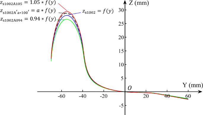

  

  S1002-based wheel profile generation

• (2) Changing $a$ will change the equivalent conicity (or RRD) of the wheelset. The increase of $a$ will lead to an increase in the equivalent conicity, thus reducing the running stability of the vehicle. On the contrary, a small $a$ results in a decrease in the equivalent conicity and an increase in lateral displacement of the wheel, resulting in the contact patch often appearing in region B (Fig. 1), which also increases the wear of wheel flange and gauge corner. In addition, a too small $a$ will reduce the flange height and increase the risk of derailment. Based on the above considerations and the author’s practical experience, in our work, $a$ is set between 0.94–1.05. This fine-tuning also allows the adaptability of the vehicle to operate on other lines.

For the vertical primary suspension stiffness

• (1) In order to ensure the load-bearing capacity of the vehicle, the total stiffness of the outer spring ($k_{\mathrm{co}}$) and the inner spring ($k_{\mathrm{ci}}$) is guaranteed to be constant, equal to the original total stiffness ($k_{\mathrm{co}} + k_{\mathrm{ci}} = 1306~\mbox{kN}/\mbox{m}$).

• (2) The outer spring stiffness cannot be removed since it needs to be used to carry the sprung mass at an empty load. It is set between 298–798 kN/m.

4.2 Simulation result

To find the optimal $a$, 12 different values ($0.94, 0.95, \dots , 1.05$) are selected (Fig. 9). To explore the influence of vertical primary suspension characteristics on wheel wear, six different vertical outer primary stiffnesses ($298, 398, \dots , 798~\mbox{kN}/\mbox{m}$) are selected. Different combinations of the two parameters are carried out to the Sgnss wagon.

Fig. 9

Selected wheel profiles for FaStrip-USFD-KSM modeling (Color figure online.)

One point that should be noted here is that the vehicle travels back and forth and is not turned at the end station. This means that the order of the wheelsets on the return trip is opposite to the order of the wheelsets on the forward trip. The wear distribution should also be arranged in reverse order. In this paper, the calculation amount is extremely large. Referring to [50], in order to shorten the simulation time, only the forward trip is considered, i.e., the wagon runs a one-way trip on the Blankenburg–Rübeland line, with a journey of 15.73 km. Finally, the wheel wear is calculated by the FaStrip-USFD method.

The result for the S1002A100 is shown in Fig. 10(a). We can know that the wear of the first wheelset (Wheel 1L + Wheel 1R) is the most pronounced, followed by the third wheelset (Wheel 3L + Wheel 3R). This is because that the first and third wheelsets are the guiding wheelsets, whose WR interaction forces are greater than the non-guiding wheelsets (second and fourth), and the front guiding wheelset (first) has a greater WR interaction force than the rear guiding wheelset (third). In addition, we can see that the wear of the left wheels (1L, 2L, 3L, and 4L) is more severe than the wear of the right wheels (1R, 2R, 3R, and 4R). It is because the proportion of the right curve is more than that of the left curve (see in Fig. 2 and Fig. 6(a)), resulting in uneven WR interaction forces between the left and right wheels and further resulting in wear differences.

Fig. 10

Wear distributions for different wheel profile: (a) S1002A100; (b) S1002A103; and (c) S1002A105 (Color figure online.)

Then, the total wear area of the eight wheels under different profiles and different vertical outer primary stiffness is generated. The results are shown in Table 3. Based on these data samples listed in Table 3, a KSM model is established. Figure 11(a) shows the response surface in a color map. Figure 11(b) shows the RMSE value of the KSM model. We can see that the RMSE value is close to 0 in the whole design space, indicating that the local error of the KSM model is small, which means that the sample selection method in our work satisfies the designing requirements described in Sect. 3.1.2.

Fig. 11

The wear area under different adjustment factors and different outer spring stiffness: (a) FaStrip-USFD-KSM model; (b) RMSE value (Color figure online.)

Table 3 Total wear area under different adjustment factors and different vertical outer spring stiffness

4.3 Model verification

Five groups of data are randomly selected to run dynamics simulations. Table 4 compares the results calculated by the FaStrip-USFD-KSM method and those obtained from the simulations (FaStrip-USFD). All the errors are lower than 6%. The simulation experiment shows that the FaStrip-USFD-KSM method can be used to select the optimal wheel profile.

Table 4 Comparison of the calculated results and simulated results

Generally, intelligent algorithms need to be applied for automatic optimization. However, the model established in this paper clearly shows that $a \approx 1.03$ (S1002A103 in Fig. 10(b)) is the optimal choice (the red line in Fig. 11), with minimal wheel wear. Therefore, the optimization calculation is omitted in this paper. However, this step is necessary in the case of high-dimensional nonlinear relationships. How to use the particle swarm optimization (PSO) algorithm for optimization calculations can be found in the authors’ previous work [53].

4.4 Analysis of result

From Table 3 and Figs. 10–13, the following two conclusions can be obtained:

• (1) The profile adjustment factor ($a$) has a large influence on the wheel wear and there is no definite trend, presenting a nonlinear relationship. As shown in Fig. 10(a), when $a=1$, the flange wear is very serious, especially the flange face wear; when $a$ is increased to 1.03, the flange wear is greatly reduced (Fig. 10(b)); and when $a$ continues to increase to 1.05, the flange wear is serious again (Fig. 10(c)). The most obvious change is located on the flange face (the blue rectangles in Fig. 10). The reason for this phenomenon is that as $a$ increases, the equivalent conicity of the wheelset increases, and when the vehicle is running on a curve, the WR contact patch tends to approach or occurs in region A described in Fig. 1. When running on a small-radius curve, the flange wear is reduced. However, if the equivalent conicity is too large, the lateral displacement of the wheelset will increase, and the area of the WR contact patch will decrease, and the spin-induced sliding velocity will also increase, thereby increasing the flange wear. More importantly, in reality, there are many nonlinear variables on the track (track layout parameters), such as arc curves, transition curves, superelevation, gauge, cant, etc., as well as vehicle speed. The position of the contact patch and the distribution of wheel wear will change with different combinations of these parameters. Finally, under the combined influence of these nonlinear factors, the relationship between the wear amount and $a$ exhibits a nonlinear relationship. By modeling the actual line, a reasonable wheel profile for reducing wheel wear can be found. In the present work, an S1002A103 profile (Fig. 10(b)) is proposed for those Sgnss wagons running on Blankenburg–Rübeland line. Simulation results show that this profile can reduce flange face wear, and the total wear can be reduced by more than 50% in short-term running.

• (2) The vertical primary suspension characteristics have an influence on the wheel wear amount, which increases with the increase of the outer spring stiffness (Fig. 12). The reason for this phenomenon is that the vertical suspension characteristics can affect the angle of attack, thus affecting the WR contact properties and further affect the wear amount. To illustrate this phenomenon, a section, which consists of a straight line, a transition curve, and a circular curve, with a track gauge of 1.450 m and a cant of 1:40, is introduced here. The curvature and superelevation distributions are shown in Figs. 13(a) and 13(b), respectively. Then, three vertical primary stiffness combinations are set on the Sgnss wagon with a speed of 51 km/h to implement simulations, respectively. Since the first and third wheelsets are the guiding wheelsets, the angle of attack of these two wheelsets is shown in Fig. 13(c). It can be seen that when the outer spring stiffness is reduced (meanwhile, the inner spring stiffness is correspondingly increased), the wheelset attack angle on the transition curve and the circular curve is also reduced. The wear amount, therefore, will correspondingly reduce (Fig. 12). Based on this phenomenon, we recommend appropriately reducing the outer spring stiffness of the Y25 bogie while increasing the inner spring stiffness to reduce wheel wear.

  Fig. 12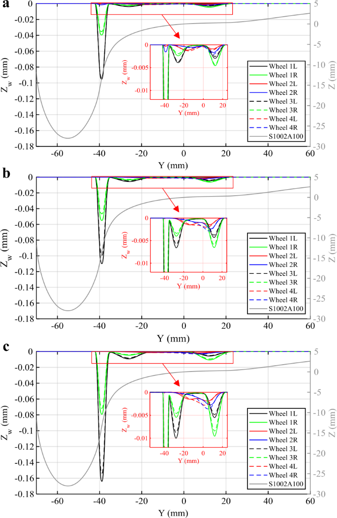

  

  Wear distributions for different vertical primary outer stiffness: (a) 298 kN/m; (b) 598 kN/m; and (c) 798 kN/m (Color figure online.)

  Fig. 13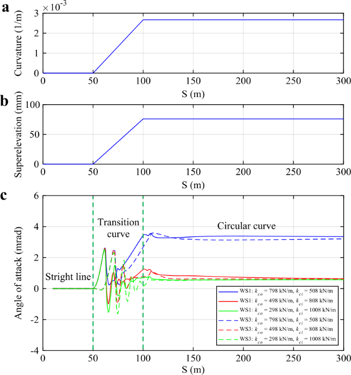

  

  Track layout distribution (a, b) and the attack angles of the first and third wheelsets (c) (Color figure online.)

4.5 Long-term wear comparison between S1002A103 and S1002 profiles

Through the above FaStrip-USFD-KSM method, it can be known that the S1002A103 wheel profile is advantageous in terms of short-term wheel wear progression for the case of this work. However, it is well known in the rail industry that the S1002 wheel profile is optimized not for the better wear performance in the short term (where there is a significant wear when the profiles are new) but for a long-term performance. To prove that the improved wheel profile (S1002A103) in the long-term wear process is still superior to the standard S1002 profile (S1002A100), in this subsection, FaStrip-USFD introduced in Sect. 3 is applied to calculate the wheel wear distribution of the Sgnss wagon after driving 5000 and 10000 km. Figure 14(a) shows a comparison between the S1002A103 and S1002A100 profiles. It can be known that the RRD and equivalent conicity is increased, this change will affect wheel wear. Figure 14(b) shows the average wear distribution of the eight wheels of the Sgnss wagon under these two wheel profiles. The simulation results show that when the optimized track is used, two advantages are produced:

• (1) The wheel flange wear is greatly reduced;

• (2) The wheel tread wear is more uniform.

Fig. 14

Comparison of S1002 and S1002A103 (a), and average wear distribution of the 8 wheels of the Sgnss wagon after driving 5000 and 10000 km (b) (Color figure online.)

To assess the operability of a wheel and to ensure the safety against derailment, in European Standard EN15313 [97], the permissible deviations of a wheel profile are defined according to three parameters: $S_{h}$ (flange height), $S_{d}$ (flange thickness), and $q_{R}$ (flange slope quota), as shown in Fig. 15. The reference points for these dimensions are a point on the nominal rolling circle and a point on the flange that is 10 mm above the measuring point on the nominal rolling circle. The limits for a 920 mm-diameter-wheel specified in EN15313 are listed in Fig. 15. Maintenance strategies such as re-profiling and scrapping are also based on these parameters.

Fig. 15

Three parameters for evaluating wheel wear as well as their limits for a 920 mm-diameter-wheel specified in EN15313

Due to the huge amount of calculation, this paper only simulates the wheel wear after driving for 10,000 km. As shown in Fig. 14, as the material loss is not serious, it is hard to accurately quantify these three parameters. However, a preliminary evaluation can be made by Fig. 14:

• In terms of $S_{h}$, it reaches the limit value faster when using the improved wheel profile S1002A103. There are two reasons for this phenomenon: (1) S1002A103 is obtained by directly multiplying the adjustment factor $a=1.03$ (Fig. 8), which increases the flange height. (2) Although the improved profile greatly reduces the flange wear and makes the tread wear more uniform, it also increases the wear depth at the nominal rolling circle to some extent.

• In terms of $S_{d}$ and $q_{R}$, the use of the improved profile has significant advantages since the flange wear is significantly reduced, which makes these two values change slowly.

Considering that during the re-profiling process, severe flange wear often leads to deeper turning depth. The S1002A103 wheel profile, therefore, is more suitable for the case of this work than the standard S1002 wheel profile from the perspective of reducing wheel wear and extending wheel service life.

5 Quasi–static and dynamic tests for the optimized wheel profile according to EN 14363

Considering the allocation of dispatching or transportation tasks, the vehicles sometimes may be transferred to other railway lines, and thus the adaptability of the vehicle needs to be guaranteed. Therefore, the derailment and running safety of the optimized wheel profile should satisfy the requirements specified in EN14363 [98]. In this section, the quasi-static safety against derailment on twisted track and the running safety on straight track are presented.

5.1 Quasi-static safety against derailment on twisted track

The quasi-static analysis is carried out in accordance with Method 1 designed in EN 14363. The vehicle must negotiate a 150-m-radius twist track without the wheel lift of the outer leading wheel exceeding 5 mm. As shown in Fig. 16 (a), the twisted track modeled in this work consists of the following parts:

• a straight line of 6 m

• a 100 m long transition curve with the end radius of 150 m

• a 430 m long full arch with a radius of 150 m

• a straight line of 30 m

Fig. 16

Track layout used in the simulation model of the twisted track (a, b) and distribution of the gaskets (c) [66]

The twist $g$ should be determined by the wheelbase distance and the pivot distance between bogies, where a constant twist of $g_{0} =3 \permil$ is used to model the track. As shown in Fig. 16 (b), the superelevation changes from +45 to −45 mm with the length of 30 m. The twist deficiency is balanced by the additional “gaskets” added under the primary or secondary springs. The thicknesses of the gaskets are calculated by the following formulas:

• Wheelbase distance $2 a^{+} \leq 4\ \text{m}$: $g_{\lim }^{+} =7\permil$

• Pivot distance $4~\mbox{m} \leq 2 a^{*} \leq 20\ \text{mm}$: $g_{\lim }^{*} = {20} / {2 a^{*}} +2=4.5\permil$

From the required test conditions, the necessary twisting thicknesses need to be calculated.

• Bogie: $h^{+} = ( g^{+} - g^{0} ) 2 a ^{+} = ( 7\permil -3\permil ) \times 1.8\ \text{m}=7.2\ \text{mm}$

• Carbody: $h^{*} = ( g^{*} - g^{0} ) 2 a ^{+} = ( 4.5\permil -3\permil ) \times 14.2\ \text{m}=21.3\ \text{mm}$

The twisting thicknesses are converted according to the lateral distances of the primary suspension of $2 b^{+}$, the secondary suspension $2 b^{*}$ and the WR contact points $2 b_{A}$:

• For the bogie twisting test: $d^{+} = {h^{+} b^{+}} / {(2 b_{A} )} = {7.2} / {1.45} =4.97\ \text{mm}$

• For the car body twisting test: $d^{*} = {h^{*} b ^{*}} / {(2 b_{A} )} = {21.3\times 0.85} / {1.45} =12.49\ \text{mm}$

The gaskets with thicknesses $d^{+}$ and $d^{*}$ are added separately under the primary and secondary suspensions, see Fig. 16(c). The used Sgnss wagon does not have secondary suspensions. Therefore, all the gaskets are added under the corresponding primary spring. The vehicle speed is set as 5 km/h.

The evaluation criterium is the maximum value $\Delta Z_{\max }$ of the wheel lift of the curve-outer wheel of the leading wheelset. The limit value is $\Delta Z_{\max } <\Delta Z_{\lim } =5\ \text{mm}$. As shown in Fig. 17, although the S1002A103 profile has a slight increase in wheel lift on the twisted curved track, it is well below the limit value (Fig. 17(a)). In addition, the $Y/Q$ ratio is introduced as an auxiliary evaluation index. Figure 17(b) shows that the $Y/Q$ ratio of the S1002A103 profile is almost the same as that of the standard S1002 profile, and both are below 1.2.

Fig. 17

Comparison of wheel lift (a) and derailment quotient $Y/Q$ (b) between S1002A100 and S1002A103 (Color figure online.)

5.2 Running safety—stability

The assessment of running stability has been carried out in two ways, by estimating the nonlinear critical speeds using the deceleration method [99] and by comparing the RMS-values of the track shifting force $\sum Y_{\mathrm{RMS}}$ at different speeds. In the deceleration method, wheelset lateral displacement is considered as the assessment criterion, it is shown in Fig. 18. The simulation runs show that the S1002A103 profile has a critical speed of about 81 km/h, while the standard one (S1002A100) has a critical speed of about 91 km/h. The reason for this phenomenon is that, when $a$ is increased, the equivalent conicity of the wheelset will also increase, resulting in a decrease in its critical speed. However, this reduction is acceptable since the maximum vehicle speed ($V_{\max } =51\ \text{km}/\text{h}$, see in Fig. 3) in our work is less than 81 km/h.

Fig. 18

Simulations run with decreasing speeds for the S1002A100 (a) and S1002A103 (b)

Another assessment criterion is the track shifting force, that is applied for track tests in the standard EN 14363. The empty wagon runs with a predefined speed on a straight track with track irregularities. The selected test speeds consider the common admissible speeds of freight wagons, namely 120 and 100 km/h, and estimated the critical speed of the S1002A100 profile of 91 km/h. For the admissible speed of 120 km/h, the test speed is 132 km/h (i.e., $V_{\mathrm{test}} =1.1 * V _{\mathrm{adm}}$). For the admissible speed of 100 km/h, the test speed is 110 km/h (i.e., $V_{\mathrm{test}} = V_{\mathrm{adm}} + 10$). Table 5 shows that the S1002A103 profile has a slightly higher $\sum Y_{ \mathrm{RMS}}$ than the standard one regardless of vehicle speeds. However, this slight increase can be neglectable since it does not affect the running safety. In addition, both profiles exceed the limit values at the speed of 132 km/h, because this speed has exceeded the allowable running speed.

Table 5 Simulation results of RMS values of the track shifting force $\sum Y_{\mathrm{RMS}}$

All in all, the quasi-static and dynamic test results show that the S1002A103 profile meets the criteria of EN14363. Tests for the suspension characteristics are omitted here. More information concerning the test can be found in the authors’ previous work [100].

6 Conclusion and discussion

With the expansion of urbanization, as well as some unique geographic or economic reasons. More and more railway vehicles shuttle on fixed lines. For these vehicles, the traditional wheel profile designing method may not be the optimal choice since they do not consider the detailed track layout parameters that have an influence on the wheel and/or rail wear. From the perspective of reducing wheel wear, this paper proposes a FaStrip-USFD-KSM based wheel profile optimization method for these vehicles that mainly run on specific lines. The following conclusions are obtained:

• (1) For those vehicles that mainly operate on fixed lines, a FaStrip-USFD-KSM based model for optimizing the wheel profile and vehicle suspension to reduce wheel wear is proposed. This method considers the track layout parameters, such as arc curves, transition curves, superelevation, gauges, and cant. In our work, an Sgnss wagon running on the German Blankenburg–Rübeland line is introduced as a case study, and an S1002A103 wheel profile is presented. Simulation results show that this profile can significantly reduce the flange face wear.

• (2) Considering the allocation of dispatching or transportation tasks, the vehicles that primarily run on special lines, sometimes, may be transferred to other railway lines, and thus the adaptability of the vehicle needs to be guaranteed. The result shows that the S1002A103 profile satisfies the derailment and running safety requirements specified in EN14363.

• (3) Based on the S1002 profile, an adjustment factor is proposed to optimize the wheel profile. This method simplifies complex curve design problems by using classical transition curves.

Besides, regarding the influence of vehicle suspension characteristics on wheel wear, most of the studies have studied the lateral stiffness, longitudinal stiffness, and yaw damper characteristics of suspension systems, since these parameters have an obvious influence on the WR wear. However, there is currently little research on the relationship between the vertical suspension characteristics and wheel wear. Therefore, it is also investigated in this paper, and the following conclusion is obtained:

• (1) The vertical primary suspension characteristics have an influence on the amount of wear, which increases with the increase of the outer spring stiffness. Based on this conclusion, we recommend appropriately reducing the outer spring stiffness of the Y25 bogie while increasing the inner spring stiffness to reduce wheel wear.

There are three points worth mentioning here.

• (1) Further field experiment verification is required.

• (2) In this paper, the optimization of the wheel profile is to multiply the $Z$-axis of the wheel profile by an adjustment factor, which increases the flange height. The wheel profile generation method, as well as the mechanism analysis, will continue to be improved in the follow-up work.

• (3) Vertical primary suspension characteristics have an influence on the amount of wear. The reason for this phenomenon is that the vertical suspension characteristics can affect the angle of attack, thus affecting the WR contact properties and further affect the wear amount. The authors will conduct an in-depth analysis on this part in future work, and the influence of the other suspension parameters on wheel wear will also be investigated.

References

Pombo, J., Ambrósio, J., Pereira, M., Lewis, R., Dwyer-Joyce, R., Ariaudo, C., et al.: Development of a wear prediction tool for steel railway wheels using three alternative wear functions. Wear 271, 238–245 (2011). https://doi.org/10.1016/j.wear.2010.10.072
Lewis, R., Olofsson, U.: Wheel–Rail Interface Handbook. CRC/Taylor & Francis, Boca Raton (2009)
Iwnicki, S.: Handbook of Railway Vehicle Dynamics. CRC/Taylor & Francis, Boca Raton (2006)
Fergusson, S.N., Fröhling, R.D., Klopper, H.: Minimising wheel wear by optimizing the primary suspension stiffness and centre plate friction of self-steering bogies. Veh. Syst. Dyn. 46(S1), 457–468 (2008). https://doi.org/10.1080/00423110801993094
Mazzola, L., Alfi, S., Bruni, S.: A method to optimise stability and wheel wear in railway bogies. Int. J. Railw. 3(3), 95–105 (2010)
Bideleh, S.M.M., Berbyuk, V., Persson, R.: Wear/comfort Pareto optimisation of bogie suspension. Veh. Syst. Dyn. 54(8), 1053–1076 (2016). https://doi.org/10.1080/00423114.2016.1180405
Bideleh, S.M.M., Berbyuk, V.: Global sensitivity analysis of bogie dynamics with respect to suspension components. Multibody Syst. Dyn. 37, 145–174 (2016). https://doi.org/10.1007/s11044-015-9497-0
Firlik, B., Staśkiewicz, T., Jaśkowski, W., Wittenbeck, L.: Optimisation of a tram wheel profile using a biologically inspired algorithm. Wear 430–431, 12–24 (2019). https://doi.org/10.1016/j.wear.2019.04.012
Polach, O.: Wheel profile design for target conicity and wide tread wear spreading. Wear 271, 195–202 (2011). https://doi.org/10.1016/j.wear.2010.10.055
Sadeghi, J., Sadeghi, S., Niaki, S.T.A.: Optimizing a hybrid vendor-managed inventory and transportation problem with fuzzy demand: an improved particle swarm optimization algorithm. Inf. Sci. 272, 126–144 (2014). https://doi.org/10.1016/j.ins.2014.02.075
Santamaria, J., Herreros, J., Vadillo, E.G., Correa, N.: Design of an optimised wheel profile for rail vehicles operating on two-track gauges. Veh. Syst. Dyn. 51, 54–73 (2013). https://doi.org/10.1080/00423114.2012.711478
Persson, I., Iwnicki, S.D.: Optimisation of railway profiles using a genetic algorithm. Veh. Syst. Dyn. 41, 517–527 (2004)
Choi, H.Y., Lee, D.H., Lee, J.: Optimisation of a railway wheel profile to minimize flange wear and surface fatigue. Wear 300, 225–233 (2013). https://doi.org/10.1016/j.wear.2013.02.009
Novales, M., Orro, A., Bugarín, M.R.: Use of a genetic algorithm to optimise wheel profile geometry. Proc. Inst. Mech. Eng., F J. Rail Rapid Transit 221, 467–476 (2007). https://doi.org/10.1243/09544097jrrt150
Kennedy, J., Eberhart, R.: Particle swarm optimization. In: Proceedings of IEEE International Conference on Neural Networks, vol. 4, pp. 1942–1948 (1995). https://doi.org/10.1109/ICNN.1995.488968
Lin, F., Zhou, S., Dong, X., Xiao, Q., Zhang, H., Hu, W., et al.: Design method of LM thin flange wheel profile based on NURBS. Veh. Syst. Dyn. 114, 1–16 (2019). https://doi.org/10.1080/00423114.2019.1657908
Cui, D., Wang, R., Allen, P., An, B., li, L., Wen, Z.: Multi-objective optimization of electric multiple unit wheel profile from wheel flange wear viewpoint. Struct. Multidiscip. Optim. 59, 279–289 (2018). https://doi.org/10.1007/s00158-018-2065-5
Shevtsov, I., Markine, V., Esveld, C.: Optimal design of wheel profile for railway vehicles. Wear 258, 1022–1030 (2005). https://doi.org/10.1016/j.wear.2004.03.051
Shevtsov, I., Markine, V., Esveld, C.: Design of railway wheel profile taking into account rolling contact fatigue and wear. Wear 265, 1273–1282 (2008). https://doi.org/10.1016/j.wear.2008.03.018
Markine, V.L., Shevtsov, I.Y.: Optimisation of a wheel profile accounting for design robustness. Proc. Inst. Mech. Eng., F J. Rail Rapid Transit 225, 433–442 (2011). https://doi.org/10.1177/09544097jrrt305
Jahed, H., Farshi, B., Eshraghi, M.A., Nasr, A.: A numerical optimisation technique for design of wheel profiles. Wear 264, 1–10 (2008). https://doi.org/10.1016/j.wear.2006.06.006
Spangenberg, U., Fröhling, R.D., Els, P.S.: Long-term wear and rolling contact fatigue behaviour of a conformal wheel profile designed for large radius curves. Veh. Syst. Dyn. 57, 44–63 (2018). https://doi.org/10.1080/00423114.2018.1447677
Shen, G., Ayasse, J.B., Chollet, H., Pratt, I.: A unique design method for wheel profiles by considering the contact angle function. Proc. Inst. Mech. Eng., F J. Rail Rapid Transit 217, 25–30 (2003). https://doi.org/10.1243/095440903762727320
Cui, D., Li, L., Jin, X., Li, X.: Optimal design of wheel profiles based on weighed wheel/rail gap. Wear 271, 218–226 (2011). https://doi.org/10.1016/j.wear.2010.10.005
Ignesti, M., Innocenti, A., Marini, L., Meli, E., Rindi, A.: Development of a wear model for the wheel profile optimisation on railway vehicles. Veh. Syst. Dyn. 51(9), 1363–1402 (2013). https://doi.org/10.1080/00423114.2013.802096
Zakharov, S., Goryacheva, I., Bogdanov, V., Pogorelov, D., Zharov, I., Yazykov, V., et al.: Problems with wheel and rail profiles selection and optimisation. Wear 265, 1266–1272 (2008). https://doi.org/10.1016/j.wear.2008.03.026
Molatefi, H., Mazraeh, A., Shadfar, M., Yazdani, H.: Advances in Iran railway wheel wear management: a practical approach for selection of wheel profile using numerical methods and comprehensive field tests. Wear 424–425, 97–110 (2019). https://doi.org/10.1016/j.wear.2019.02.016
Ashtiani, I.H.: Optimization of secondary suspension of three-piece bogie with bevelled friction wedge geometry. Int. J. Railw. Technol. Transp. 5, 213–228 (2017). https://doi.org/10.1080/23248378.2017.1336652
Ashtiani, I.H., Rakheja, S., Ahmed, A.: Influence of friction wedge characteristics on lateral response and hunting of freight wagons with three-piece bogies. Proc. Inst. Mech. Eng., F J. Rail Rapid Transit 231, 877–891 (2016). https://doi.org/10.1177/0954409716647095
Liu, B., Mei, T., Bruni, S.: Design and optimisation of wheel–rail profiles for adhesion improvement. Veh. Syst. Dyn. 54, 429–444 (2016). https://doi.org/10.1080/00423114.2015.1137958
Pombo, J., Ambrósio, J., Pereira, M., Lewis, R., Dwyer-Joyce, R., Ariaudo, C., et al.: A study on wear evaluation of railway wheels based on multibody dynamics and wear computation. Multibody Syst. Dyn. 24, 347–366 (2010). https://doi.org/10.1007/s11044-010-9217-8
Gao, L., Wang, P., Cai, X., Xiao, H.: Superelevation modification for the small-radius curve of Shen-shuo railway under mixed traffic of passenger and freight trains. J. Vib. Shock 35, 222–228 (2018). https://doi.org/10.13465/j.cnki.jvs.2016.14.036 (in Chinese)
Ye, Y., Ning, J.: Small-amplitude hunting diagnosis method for high-speed trains based on the bogie frame’s lateral–longitudinal–vertical data fusion, independent mode function reconstruction and linear local tangent space alignment. Proceedings of the Institution of Mechanical Engineers, Part F: Journal of Rail and Rapid Transit., 095440971882541 (2019). https://doi.org/10.1177/0954409718825412
Rongju, T.: The development of China’s railway building. Transp. Rev. 4(1), 27–42 (1984). https://doi.org/10.1080/01441648408716543
Eisenbahn Freunde–Warstein. https://eisenbahnfreunde-warstein.hpage.com/willkommen.html
Schelle, H.: Radverschleißreduzierung für eine Güterzuglokomotive durch optimierte Spurführung. (Doctoral dissertation), Technische Universität Berlin (2014)
Tao, G., Ren, D., Wang, L., Wen, Z., Jin, X.: Online prediction model for wheel wear considering track flexibility. Multibody Syst. Dyn. 44, 313–334 (2018)
Ignesti, M., Innocenti, A., Marini, L., Meli, E., Rindi, A.: Development of a model for the simultaneous analysis of wheel and rail wear in railway systems. Multibody Syst. Dyn. 31, 191–240 (2014)
An, B., Wang, P., Zhou, J., Chen, R., Xu, J., Wu, B.: Applying two simplified ellipse-based tangential models to wheel–rail contact using three alternative nonelliptic adaptation approaches: a comparative study. Math. Probl. Eng. 2019, 1–17 (2019). https://doi.org/10.1155/2019/3478607
Johnson, K.L.: Contact Mechanics. Cambridge University Press, Cambridge (2004)
Tao, G., Wen, Z., Zhao, X., Jin, X.: Effects of wheel–rail contact modelling on wheel wear simulation. Wear 366–367, 146–156 (2016). https://doi.org/10.1016/j.wear.2016.05.010
Shen, Z.Y., Hedrick, J.K., Elkins, J.A.: A comparison of alternative creep force models for rail vehicle dynamic analysis. Veh. Syst. Dyn. 12, 79–83 (1983). https://doi.org/10.1080/00423118308968725
Polach, O.: A fast wheel–rail forces calculation computer code. Veh. Syst. Dyn. 33, 728–739 (2000)
Kalker, J.J.: A fast algorithm for the simplified theory of rolling contact. Veh. Syst. Dyn. 11, 1–13 (1982). https://doi.org/10.1080/00423118208968684
Sichani, M.S., Enblom, R., Berg, M.: An alternative to FASTSIM for tangential solution of the wheel–rail contact. Veh. Syst. Dyn. 54, 748–764 (2016). https://doi.org/10.1080/00423114.2016.1156135
Auciello, J., Ignesti, M., Malvezzi, M., Meli, E., Rindi, A.: Development and validation of a wear model for the analysis of the wheel profile evolution in railway vehicles. Veh. Syst. Dyn. 50, 1707–1734 (2012). https://doi.org/10.1080/00423114.2012.695021
Sun, Y., Guo, Y., Zhai, W.: Prediction of rail non-uniform wear–influence of track random irregularity. Wear 420–421, 235–244 (2019)
Peng, B., Iwnicki, S., Shackleton, P., Crosbee, D.: Comparison of wear models for simulation of railway wheel polygonization. Wear 436–437, 203010 (2019). https://doi.org/10.1016/j.wear.2019.203010
Archard, J.F.: Contact and rubbing of flat surfaces. J. Appl. Phys. 24, 981–988 (1953)
Jendel, T.: Prediction of wheel profile wear—comparisons with field measurements. Wear 253, 89–99 (2002). https://doi.org/10.1016/s0043-1648(02)00087-x
Pearce, T., Sherratt, N.: Prediction of wheel profile wear. Wear 144, 343–351 (1991). https://doi.org/10.1016/0043-1648(91)90025-p
Lewis, R., Dwyer-Joyce, R.S., Olofsson, U., Pombo, J., Ambrósio, J., Pereira, M., Ariaudo, C., Kuka, N.: Mapping railway wheel material wear mechanisms and transitions. Proc. Inst. Mech. Eng., F J. Rail Rapid Transit 224, 125–137 (2010)
Ye, Y., Shi, D., Krause, P., Hecht, M.: A data-driven method for estimating wheel flat length. Veh. Syst. Dyn. 304, 1–19 (2019). https://doi.org/10.1080/00423114.2019.1620956
Chowdhury, R., Adhikari, S.: Fuzzy parametric uncertainty analysis of linear dynamical systems: a surrogate modeling approach. Mech. Syst. Signal Process. 32, 5–17 (2012). https://doi.org/10.1016/j.ymssp.2012.05.002
Nie, Y., Tang, Z., Liu, F., Chang, J., Zhang, J.: A data-driven dynamics simulation framework for railway vehicles. Veh. Syst. Dyn. 56, 406–427 (2017). https://doi.org/10.1080/00423114.2017.1381981
Simpson, T.W., Mauery, T.M., Korte, J., Mistree, F.: Kriging models for global approximation in simulation-based multidisciplinary design optimization. AIAA J. 39, 2233–2241 (2001). https://doi.org/10.2514/3.15017
Werner, R., Lauschmann, S., Ehms, H.: Betrieb mit 25 kV 50 Hz auf den Steilstrecken der Rübelandbahn im Harz. Elektr. Bahnen Verkehrssysteme 107(10), 413–425 (2009)
European Commission. https://cordis.europa.eu/project/rcn/92249/reporting/en
Deutsche Reichsbahn: Strecke Blankenburg—Tanne. Entwurfs- und Vermessungsstelle der Deutschen Reichsbahn, Magdeburg (1965)
Pfeiffer, M., Hecht, M.: Concept & Decision Paper: force measurement method for ED-brake-monitoring (Electric Locomotive—BOMBARDIER TRAXX) incl. data analysis—Measurement campaign HVLE. (Report No. 11/2011), Technische Universität Berlin (2011)
Profillidis, V.A.: Railway Engineering. Avebury Technical, Aldershot (2000)
Olofsson, U., Sundvall, K.: Influence of leaf, humidity and applied lubrication on friction in the wheel–rail contact: pin-on-disc experiments. Proc. Inst. Mech. Eng., F J. Rail Rapid Transit 218, 235–242 (2004). https://doi.org/10.1243/0954409042389364
Kovalev, R., Lysikov, N., Mikheev, G., Pogorelov, D., Simonov, V., Yazykov, V., et al.: Freight car models and their computer-aided dynamic analysis. Multibody Syst. Dyn. 22, 399–423 (2009). https://doi.org/10.1007/s11044-009-9170-6
Hecht, M., Keudel, J., Friedrich, D.: Dokumentation der Messfahrten aus Juni 2006. (Report No. 12/2006), Technische Universität Berlin. (2006)
Hecht, M., Keudel, J.: Numerische Simulation eines Selbstentladewagens mit Y25-Drehgestellen. (Report No. 31/2005) (2005)
Hecht, M., Schelle, H.: Simulation von Kesselwagen mit Y25-Drehgestellen bei Gleislagefehlern. Technische Universität Berlin (2006) (Report No. 16/2006)
Enblom, R.: Deterioration mechanisms in the wheel–rail interface with focus on wear prediction: a literature review. Veh. Syst. Dyn. 47, 661–700 (2009). https://doi.org/10.1080/00423110802331559
Tao, G.Q., Du, X., Wen, Z.F., Jin, X.S., Cui, D.B.: Development and validation of a model for predicting wheel wear in high-speed trains. J. Zhejiang Univ. Sci. A 18, 603–616 (2017)
Braghin, F., Lewis, R., Dwyer-Joyce, R., Bruni, S.: A mathematical model to predict railway wheel profile evolution due to wear. Wear 261, 1253–1264 (2006). https://doi.org/10.1016/j.wear.2006.03.025
Luo, R., Shi, H., Teng, W., Song, C.: Prediction of wheel profile wear and vehicle dynamics evolution considering stochastic parameters for high-speed train. Wear 392–393, 126–138 (2017). https://doi.org/10.1016/j.wear.2017.09.019
Enblom, R., Berg, M.: Simulation of railway wheel profile development due to wear—influence of disc braking and contact environment. Wear 258, 1055–1063 (2005). https://doi.org/10.1016/j.wear.2004.03.055
Braghin, F., Bruni, S., Resta, F.: Wear of railway wheel profiles: a comparison between experimental results and a mathematical model. Veh. Syst. Dyn. 37, 478–489 (2002). https://doi.org/10.1080/00423114.2002.11666256
Sun, Y., Guo, Y., Lv, K., Chen, M., Zhai, W.: Effect of hollow-worn wheels on the evolution of rail wear. Wear 436–437, 203032 (2019). https://doi.org/10.1016/j.wear.2019.203032
Meymand, S.Z., Keylin, A., Ahmadian, M.: A survey of wheel–rail contact models for rail vehicles. Veh. Syst. Dyn. 54, 386–428 (2016). https://doi.org/10.1080/00423114.2015.1137956
Laursen, T.: Computational Contact and Impact Mechanics, Fundamentals of Modeling Interfacial Phenomena in Nonlinear Finite Element Analysis. Springer, Berlin (2002)
Nackenhorst, U.: The ALE-formulation of bodies in rolling contact. Comput. Methods Appl. Mech. Eng. 193, 4299–4322 (2004). https://doi.org/10.1016/j.cma.2004.01.033
Vollebregt, E., Segal, G.: Solving conformal wheel–rail rolling contact problems. Veh. Syst. Dyn. 52, 455–468 (2014). https://doi.org/10.1080/00423114.2014.906634
Burgelman, N., Li, Z., Dollevoet, R.: A new rolling contact method applied to conformal contact and the train–turnout interaction. Wear 321, 94–105 (2014). https://doi.org/10.1016/j.wear.2014.10.008
Kalker, J.J.: Three-Dimensional Elastic Bodies in Rolling Contact. Solid Mechanics and Its Applications, vol. 2. Kluwer Academic Publishers, Dordrecht (1990)
Linder, C.: Verschleiß von Eisenbahnrädern mit Unrundheiten. Dissertation Nr. 12342, ETH, Zurich (1997)
Piotrowski, J., Kik, W.: A simplified model of wheel/rail contact mechanics for non-hertzian problems and its application in rail vehicle dynamic simulations. Veh. Syst. Dyn. 46, 27–48 (2008). https://doi.org/10.1080/00423110701586444
Liu, B., Bruni, S., Vollebregt, E.: A non-hertzian method for solving wheel–rail normal contact problem taking into account the effect of yaw. Veh. Syst. Dyn. 54, 1226–1246 (2016). https://doi.org/10.1080/00423114.2016.1196823
Sun, Y., Zhai, W., Guo, Y.: A robust non-hertzian contact method for wheel–rail normal contact analysis. Veh. Syst. Dyn. 56, 1899–1921 (2018). https://doi.org/10.1080/00423114.2018.1439587
Ayasse, J., Chollet, H.: Determination of the wheel rail contact patch in semi-hertzian conditions. Veh. Syst. Dyn. 43, 161–172 (2005). https://doi.org/10.1080/00423110412331327193
Sichani, M.S., Enblom, R., Berg, M.: A novel method to model wheel–rail normal contact in vehicle dynamics simulation. Veh. Syst. Dyn. 52, 1752–1764 (2014). https://doi.org/10.1080/00423114.2014.961932
Magalhães, H., Marques, F., Liu, B., Antunes, P., Pombo, J., Flores, P., et al.: Implementation of a non-hertzian contact model for railway dynamic application. In: Multibody System Dynamics (2019). https://doi.org/10.1007/s11044-019-09688-y
Marques, F., Magalhães, H., Liu, B., Pombo, J., Flores, P., Ambrósio, J., et al.: On the generation of enhanced lookup tables for wheel–rail contact models. Wear 434–435, 202993 (2019). https://doi.org/10.1016/j.wear.2019.202993
Kalker, J.J.: Rollin contact phenomena—linear elasticity. In: Jacobson, B., Kalker, J. (eds.) Rolling Contact Phenomena. CISM Courses and Lectures, pp. 1–84. Springer, New York (2001)
Hossein-Nia, S., Sichani, M.S., Stichel, S., Casanueva, C.: Wheel life prediction model—an alternative to the FASTSIM algorithm for RCF. Veh. Syst. Dyn. 56, 1051–1071 (2017). https://doi.org/10.1080/00423114.2017.1403636
An, B., Ma, D., Wang, P., Zhou, J., Chen, R., Xu, J., et al.: Assessing the fast non-Hertzian methods based on the simulation of wheel–rail rolling contact and wear distribution. Proceedings of the Institution of Mechanical Engineers, Part F: Journal of Rail and Rapid Transit. 095440971984859 (2019). https://doi.org/10.1177/0954409719848592
Kalker, J.J.: A Strip Theory for Rolling with Slip and Spin. TU Delft, Delft (1966)
Ye, Y., Shi, D., Krause, P., Tian, Q., Hecht, M.: Wheel flat can cause or exacerbate wheel polygonization. Veh. Syst. Dyn. (2019). https://doi.org/10.1080/00423114.2019.1636098
Johansson, A.: Out-of-round railway wheels—causes and consequences. (Doctoral thesis), Chalmers University of Technology, Sweden (2005)
E, J., Han, D., Qiu, A., Zhu, H., Deng, Y., Chen, J., et al.: Orthogonal experimental design of liquid-cooling structure on the cooling effect of a liquid-cooled battery thermal management system. Appl. Therm. Eng. 132, 508–520 (2018). https://doi.org/10.1016/j.applthermaleng.2017.12.115
Roshanian, J., Ebrahimi, M.: Latin hypercube sampling applied to reliability-based multidisciplinary design optimization of a launch vehicle. Aerosp. Sci. Technol. 28, 297–304 (2013). https://doi.org/10.1016/j.ast.2012.11.010
Xin, C., Lu, Q., Ai, C., Rahman, A., Qiu, Y.: Optimization of hard modified asphalt formula for gussasphalt based on uniform experimental design. Constr. Build. Mater. 136, 556–564 (2017). https://doi.org/10.1016/j.conbuildmat.2017.01.068
BS EN 15313: Railway applications. In-service wheelset operation requirements. In-service and off-vehicle wheelset maintenance (2016). https://standards.globalspec.com/std/10011238/dsf-en-15313-pra1
BS EN 14363: Railway Applications-Testing for the Acceptance of Running Characteristics of Railway Vehicles-Testing of Running Behavior and Stationary Tests. CEN, Brussels (2005). https://standards.globalspec.com/std/13162966/en-14363
Polach, O.: On non-linear methods of bogie stability assessment using computer simulations. Proc. Inst. Mech. Eng., F J. Rail Rapid Transit 220, 13–27 (2006). https://doi.org/10.1243/095440905x33251
Ye, Y.G., Hecht, H.: Derailment safety and stability behavior tests of Y25-container wagon with wheel diameter decreasing from 920 mm to 550 mm. (Report No. 11/2018), Technische Universität Berlin (2018)
Zhang, Y., Zhou, S., Zhang, G., Chang, C., Zhou, Q., Wang, W.: Study and discussion of high speed wheel-rail hardness matching. China Railw. 1, 7–14 (2018). (In Chinese). http://www.cnki.com.cn/Article/CJFDTotal-TLZG201801002.htm
Knothe, K., Stichel, S.: Rail Vehicle Dynamics. Springer, Berlin (2018)
Acknowledgements
Open Access funding provided by Projekt DEAL. This study is supported by the Assets4Rail project which is funded by the Shift2Rail Joint Undertaking under the EU’s H2020 program (Grant No.: 826250), and part of the experiment data concerning the railway line and the Sgnss wagon used in this paper is supported by the DynoTRAIN project, funded by European Commission (Grant No.: 234079). The first author is also supported by China Scholarship Council (Grant No.: 201707000113). The authors would like to thank Dr. Henning Schelle for the collection of the data. The authors would like to thank Dr. Boyang An from Southwest Jiaotong University for his valuable advice on WR contact calculation.
Author information
Authors and Affiliations
Corresponding authors
Ethics declarations
Declaration of interests
The authors declare that they have no conflicts of interest.
Replication of results
In this work, the 3D geometry of the bogie frame and axlebox was modeled in INVENTOR, noting that these geometrical appearances did not affect the dynamics calculations. The track model and whole vehicle model, as well as the vehicle dynamics analysis, were performed in SIMPACK. The wheel wear simulation was performed by SIMPACK/MATLAB co-simulation. The KSM was performed in MATLAB. The unlisted data about the track is confidential and the authors have no right to provide it. However, readers interested in the internal reports (in German) listed in this article, as well as the MATLAB codes, are encouraged to contact the corresponding authors by e-mail.
Additional information
Publisher’s Note
Springer Nature remains neutral with regard to jurisdictional claims in published maps and institutional affiliations.
Rights and permissions
Open Access This article is licensed under a Creative Commons Attribution 4.0 International License, which permits use, sharing, adaptation, distribution and reproduction in any medium or format, as long as you give appropriate credit to the original author(s) and the source, provide a link to the Creative Commons licence, and indicate if changes were made. The images or other third party material in this article are included in the article’s Creative Commons licence, unless indicated otherwise in a credit line to the material. If material is not included in the article’s Creative Commons licence and your intended use is not permitted by statutory regulation or exceeds the permitted use, you will need to obtain permission directly from the copyright holder. To view a copy of this licence, visit http://creativecommons.org/licenses/by/4.0/.
About this article
Cite this article
Ye, Y., Sun, Y., Dongfang, S. et al. Optimizing wheel profiles and suspensions for railway vehicles operating on specific lines to reduce wheel wear: a case study. Multibody Syst Dyn 51, 91–122 (2021). https://doi.org/10.1007/s11044-020-09722-4
Received:
Accepted:
Published:
Issue Date:
DOI: https://doi.org/10.1007/s11044-020-09722-4