Deep reinforcement learning based control for Autonomous Vehicles in CARLA

Abstract

Nowadays, Artificial Intelligence (AI) is growing by leaps and bounds in almost all fields of technology, and Autonomous Vehicles (AV) research is one more of them. This paper proposes the using of algorithms based on Deep Learning (DL) in the control layer of an autonomous vehicle. More specifically, Deep Reinforcement Learning (DRL) algorithms such as Deep Q-Network (DQN) and Deep Deterministic Policy Gradient (DDPG) are implemented in order to compare results between them. The aim of this work is to obtain a trained model, applying a DRL algorithm, able of sending control commands to the vehicle to navigate properly and efficiently following a determined route. In addition, for each of the algorithms, several agents are presented as a solution, so that each of these agents uses different data sources to achieve the vehicle control commands. For this purpose, an open-source simulator such as CARLA is used, providing to the system with the ability to perform a multitude of tests without any risk into an hyper-realistic urban simulation environment, something that is unthinkable in the real world. The results obtained show that both DQN and DDPG reach the goal, but DDPG obtains a better performance. DDPG perfoms trajectories very similar to classic controller as LQR. In both cases RMSE is lower than 0.1m following trajectories with a range 180-700m. To conclude, some conclusions and future works are commented.

1 Introduction

In recent years, autonomous driving plays a pivotal role to solve traffic and transportation problems in urban areas (traffic congestions, accidents, etc) and it is going to change the way of travelling in our world in the future [5]. In the last decade, various challenges, such as the well-known DARPA Urban Challenge and the Intelligent Vehicle Future Challenge (IVFC) have proven that autonomous driving can be a reality in the near future. The teams participating in these events have demonstrated numerous technical frameworks for autonomous driving [36, 43, 44, 51]. Nowadays, most self-driving vehicles are geared up with multiple high-precision sensors such as LIDAR and cameras. LIDAR-based detection methods provide accurate depth information and obtain robust results in location, object detection and scene understanding [26] while camera-based methods provide much more detailed semantic information [2].

Considering a typical AV architecture, the control layer consists of a set of processes that implements the vehicle control and navigation functionality. A well defined control layer makes the vehicle robust regardless the varying environment situations, such as the traffic participants, weather conditions or traffic scenario, on the premise of guarantying vehicle stability and covering the route provided by any global planner, assuming that the control layer is based on a previous mapping and path planning layer that loads the map and planes the route. In that sense, a large number of classic controllers as [3, 30, 38] have been successfully implemented in AV architectures.

In this context, AI is expanding through AV architecture, dealing with different processes such as detection, Multi-Object Tracking (MOT) and environment prediction, or evaluating the current situation of the ego-vehicle to conduct the safest decision, for example making use of DRL algorithms for behavioural driving [31]. DRL based algorithms have been recently used to solve Markov Decision Processes (MDPs), where the scope of the algorithm is to calculate the optimal policy of an agent to choose actions in an environment with the goal of maximize a reward function, obtaining quite successful results in fields like solving computer games [42] or simple decision-making system [35]. In terms of autonomous driving, DRL approaches have been developed to learn how to use the AV sensor suite on-board the vehicle [23, 28].

In this paper, we study the inclusion of AI techniques into the control layer, referred to classic AV control architecture, through implementation of a control based on DRL algorithms for autonomous vehicle navigation. More specifically, two different approaches will be developed, the Deep Q-Network (DQN) and the Deep Deterministic Policy Gradient (DDPG). Figure 1 shows the framework overview that has been developed in this work. The goal is to follow a predetermined route as fast as possible avoiding collisions and road departures in a dynamic urban environment in simulation. On the one hand, the discrete nature of DQN is not well studied ongoing problem like self-driving, due to the infinite possibles of movement the car in each step. Studying DQN and the obtained results, we will analyze the limitations of this method for this navigation purpose. On the other hand, the DDPG algorithm has a continuous nature that fits better to autonomous driving task. Both algorithms will be implemented in order to compare them, and then decide which could be transferred to a real vehicle. As a previous design step all algorithms will be tested in simulation by using CARLA Simulator [14]. In terms of autonomous driving, DRL approaches have been developed to learn how to use the AV sensor suite on-board the vehicle [23, 28]. The analysis of the DQN algorithm has been previously published by the authors in WAF2020 workshop [37]. This work studies the DDPG algorithm, compare results between the two methods in simulation, and prepare the best option for a real application.

Fig. 1

Framework overview

2 Related works

As mentioned in the previous section, several approaches for the control layer of an AV have been developed, which are commonly classified into classic controller and AI based controllers. The basics of control systems state that the transfer functions decides the relationship between the outputs and the inputs given the plant. While classic controllers use the system model to define their input-output relations, AI based controllers may or may not use the system model and rather manage the vehicle based on the experience they have with the system while training, as occur with Imitation Learning, or possible enhance it in real-time as well, as Reinforcement Learning. Then, the difference in terms of applicability between classic and AI based controllers is actually the difference between deterministic and stochastic behaviour. While pure conventional control techniques offer a deterministic behaviour, AI based controllers have stochastic behaviour due to the fact that they learn from a certain set of features. So the learning process can be poor depending on a lot of intrinsic and extrinsic factors, such as the model architecture, the data quality or the corresponding hyperparameters. Hereafter we present some of the most relevant algorithms used in the control layer.

2.1 Classic controllers

Classic autonomous driving systems usually use advanced sensor for environment perception and complex control algorithms for safety navigation in arbitrarily challenging scenarios. Typically, these frameworks use a modular architecture where individual modules process information asynchronously. The perception layer captures information from the surroundings using different sensors such cameras, LiDAR, RADAR, GNSS, IMU and so on. Regarding the control layer, some of most used control methods are the PID control method [6, 24], the Model Predictive Control algorithm [25], the Fuzzy Control method [9, 21], the Model-Reference Adaptive method [4, 46], the Fractional Order control method [52], the Pure-Pursuit (PP) path tracking control method [11] and the Linear-Quadratic Regulator (LQR) algorithm [20].

However, despite their good performance, these controllers are often environment dependent, so their corresponding hyperparameters must be properly fine-tuned for each environment in order to obtain the expected behaviour, which is not a trivial task to do.

2.2 Imitation learning

This approach tries to learn the optimal policy by following and imitating an expert system decisions. In that sense, an expert system (typically a human) provides a set of driving data [7, 10], which is used to train the driving policy (agent) through supervised learning. The main advantage of this method is its simplicity, since it achieves very good results in end-to-end applications (navigating from the current position to a certain goal as fast as possible avoiding collisions and road departures in an arbitrarily complex dynamic environment). Nevertheless, its main drawback is the difficulty of imitating every potential driving scene being unable to reproduce behaviors that have not been learnt. This drawback causes this approach can be dangerous in some real driving situations that have not been previously observed.

2.3 Deep reinforcement learning

While Reinforcement learning (RL) algorithms are dynamically learning with a trial and error method to maximize the outcome, being rewarded for a correct prediction and penalized for incorrect predictions, and successfully tested for solving Markov Decision Problems (MDPs). However, as illustrated above, it can be overwhelming for the algorithm to learn from all states and determine the reward path. Then, DRL based algorithms replaces tabular methods of estimating state values (need to store all possible state and value pairs) with a function approximation (the Deep prefix comes here) that enables the agent, in this case the ego-vehicle, to generalize the value of states it has never seen before, or has partial by seen, by using the values of similar states. Regarding this, the combination of Deep Learning techniques and Reinforcement Learning algorithms have demonstrated its potential solving some of the most challenging tasks of autonomous driving, such as decision making and planning [49]. Deep Reinforcement Learning (DRL) algorithms include: Deep Q-learning Network (DQN) [17, 33], Double-DQN, actor-critic (A2C, A3C) [27], Deep Deterministic Policy Gradient (DDPG) [45, 47] and Twin Delayed DDPG (TD3) [50]. Our work is focused in DQN and DDPG algorithms, which are explained in the following section.

3 Deep reinforcement learning algorithms

Deep Reinforcement Learning combines artificial neural networks with a reinforcement learning architecture that enables software-defined agents to learn the best actions possible in virtual environments in order to attain their own goals. That is, it unites function approximation and target optimization, mapping state-action pairs to expected rewards. This algorithms try to seem the human behaviour at learning time with his action-reward structure, rewarding the agent when the chosen action is good, and penalizing it in opposite case. This section is needed in order to understand how the algorithms used in our approaches work, as well as to appreciate the existing differences between them. Deep Q-Network algorithm must be explained from Q-learning and Deep Q-learning theory, while Deep Deterministic Policy Gradient is explained later based on the previous DQN explanation.

3.1 Deep Q-Network

Recently, a great amount of reinforcement learning algorithms have been developed to solve MDP [23, 33]. MDP is defined by a tuple (S, A, P, R), where S is the set of states, A is the set of actions, $P: S \; \times A \rightarrow P(S)$ is the Markov transition kernel and $R: S \times A \rightarrow P(\mathbb {R})$ is the reward distribution. So taking any action $a \in A$ at any state $s \in S$, $P(\cdot |s,a)$ defines the probability of the next state and $R(\cdot |s,a)$ is the reward distribution. A policy $\pi : S \rightarrow P(A)$ maps any state $s \in S$ to a probability distribution $\pi (\cdot |s)$ over A.

3.1.1 Q-Learning

Q-Learning algorithm [17] creates an exact matrix for the agent to maximize its reward in the long run. This approach is only practical for restricted environment, with limited space for observation, due to an increase in number of states or actions causes a wrong algorithm behaviour. Q-Learning is an off-policy, model-free RL based on the Bellman Equation, where v refers to its optimal value:

$$\begin{aligned} v(s) = E[R_{t+1} + \lambda v(S_{t+1})|S_t = s] \end{aligned}$$

(1)

E refers to the expectation, while $\lambda$ refers to the discount factor for the ahead rewards, and rewriting it in the form of Q-value:

$$\begin{aligned} Q^{\pi }(s,a) = E[r_{t+1} + \lambda r_{t+2} + \lambda ^2 r_{t+3} + ... |s,a] = E_{s'}[r + \lambda Q^{\pi }(s^\prime,a^\prime)|s,a] \end{aligned}$$

(2)

Where the optimal Q-value $Q^*$ can be expressed as:

$$\begin{aligned} Q^*(s,a) = E_{s^\prime}[r+\lambda \max _{a'}Q^*(s^\prime,a^\prime)|s,a] \end{aligned}$$

(3)

The goal of Q-Learning is to maximize the Q-value trough iteration policy, which tuns a loop between policy evaluation and policy improvement. Policy evaluation estimates the value of function V with the greedy policy, which has been obtained from the last policy improvement. On the other hand, policy improvement updates the policy with the action that maximize V function for each state. Value iteration updates the function V based on the Optimal Bellman Equation as follows:

$$\begin{aligned} v_*(s) = \max _{a}E[R_{t+1} + \gamma v_*(S_{t+1})|S_t =s, A_t =a] = \max _{a} \sum _{a^\prime,r} p(s^\prime,r|s,a)[r + \gamma v_*(s^\prime)] \end{aligned}$$

(4)

When iteration converges, the optimal policy is obtained by applying an argument of max function for all the states.

$$\begin{aligned} \pi (s) = \max _a \sum _{s^\prime,r} p(s^\prime,r|s,a)[r + \gamma V(s^\prime)] \end{aligned}$$

(5)

As result, the update equation is replaced by the following formula, where $\alpha$ refers to the learning rate:

$$\begin{aligned} Q(s_t,a_t) = Q(s_t,a_t ) + \alpha [r_t{_+}{_1} + \gamma \max _a Q(s_t{_+}{_1}, a_t) - Q(s_t,a_t )] \end{aligned}$$

(6)

3.1.2 Deep Q-Learning

As we indicated above, Q-learning lacks of generality when space of observation increases. Imagine one situation with 10 states and 10 possible actions, we have a 10x10 matrix, but if the number of states increases to 1000, the Q-matrix dramatically increases and it is difficult to manages the in a manual way. To solve this issue, Deep Q-Learning [17, 41] manage of the two-dimensional array by introducing a Neural Network. So, DQN estimates Q-values by using it in a learning process, where the state is the input of the Net, and the output is the corresponding Q-value for each action. The difference between D-Learning and Deep Q-Learning lies in the target equation y:

$$\begin{aligned} y_j = r_j + \gamma \max _a Q(s_j{_+}{_1}, a^\prime ; \theta ^-) \end{aligned}$$

(7)

Where the $\theta$ stands for the parameters in the Neural Network.

3.2 Deep deterministic policy gradient

Deep Deterministic Policy Gradient (DDPG) [15, 22, 32] is a DRL algorithm that concurrently learns a Q-function and a policy. It uses off-policy data and the Bellman equation to learn the Q-function, where the Q-function to learn is the policy.

The algorithm that learns and take the decisions is known as the agent, which is interacting with the environment. The agent is continuously choosing actions $a_i$ from an Action space $A = \mathbb {R}^N$ and a State space $s_t{_+}{_1}$, in such a way that a reward $r(s_t, a_t)$ is returned by the environment. The agent behaviour is governed by a policy ($\pi$) which plays as a state map in the action probabilistic distribution $\pi : S \rightarrow P(A)$ in a stochastic environment E.

The two main components in the policy gradient are the policy model and the value function. It makes sense to learn the value function and the policy model simultaneously, since the value function can assist the policy update by reducing the gradient variance in vanilla policy gradients, what is actually what the Actor-Critic method does. This method consists of two models (Critic and Actor), which may optionally share some parameters: While the Critic updates the value function parameters in function of the action-value, the Actor updates the policy parameters $\theta$ according to the suggestions of the Critic.

The output of a state in the State space is defined as the sum of all future rewards discounted:

$$\begin{aligned} \sum _{i=t}^{T} \gamma ^{(i-t)} r(s_i, a_i) \end{aligned}$$

(8)

Where $\gamma \in [0, 1]$ is a discount factor. Defining the action-value function as the expected value when an action $a_t$ is taken in the state $s_t$, the Q-function is used in order to follow the policy $\pi$ in the following way:

$$\begin{aligned} Q^\pi (s_t, a_t) = E_{r_i \ge t, s \ge t \sim E, a_i \ge t \sim \pi }[R_t | s_t, a_t] \end{aligned}$$

(9)

Besides this, the Bellman equation is used with a deterministic policy $\mu$:

$$\begin{aligned} A = E_{r_t,s_t{_+}{_1} \sim E} [r(s_t, a_t) \end{aligned}$$

(10)

$$\begin{aligned} B = \gamma Q^\mu (s_t{_+}{_1}, \mu (S_t +1))] \end{aligned}$$

(11)

$$\begin{aligned} Q^\mu (s_t, a_t) = A + B \end{aligned}$$

(12)

Using Eq. 12 to update the Q-function defined in Eq. 9, we define $y_t$ as the discounted reward for the current action:

$$\begin{aligned} y_t = r(s_t, a_t) + \gamma Q(s_{t+1}, \mu (s_{t+1}|\theta ^Q)) \end{aligned}$$

(13)

Then, we consider function approximators parameterized by $\theta ^Q$, which we optimize by minimizing the loss:

$$\begin{aligned} L(\theta ^Q) = E_{s_t \sim \rho ^\beta ,a_t \sim \beta , r_t \sim E} [(Q(s_t, a_t|\theta ^Q) - y_t)^2] \end{aligned}$$

(14)

Where $\beta$ represents any stochastic policy and $p^\pi$ the discounted distribution of visitation for an action probabilistic distribution $\pi$. Note that since $y_t$ also depends on $\theta ^Q$, this is typically ignored.

Finally, through these updates the function Q(s, a) of the Critic is found. The updates of the Actor are based on following the gradient of the expected value of the initial distribution J according to the parameters of the neural network of the Actor, which represents the gradient of the policy performance.

$$\begin{aligned} \nabla _{\theta ^Q} J \approx E_{s_t \sim \rho ^\beta } [\nabla _{\theta ^Q}Q(s,a|\theta ^Q)|_{s=s_t, a=\mu }(s_t|\theta ^\mu )] \end{aligned}$$

(15)

Nevertheless, despite the fact that DRL algorithms assume that independent samples follow a similar distribution, this is not true in a context where there exists an environment interaction, where following a particular state is a direct consequence of the current state and the executed action. In that sense, the DQN algorithm solves this problem by adding the experience replay method also implemented in the DDPG method. The experience replay method consists in keeping a buffer of past transitions available to update the algorithm with them. This technique not only boosts the learning process and increases the efficiency of the exploration [29, 34], but also has proven to be vital for the stability of the learning process [12]. Updating the agent using past iterations allows to evaluate a single iteration several times with different policies, increasing the efficiency of the initial exploration.

Moreover, one of the most important DQN contributions is using target networks that makes the Critic update more stable, since in the absence of target networks, an update used to increase the value of $Q(s_t, a_t)$ and $Q(s_{t+1},a )$, creates a bias that can lead to oscillations or even divergence in the policy value. To deal with this problem, we modify the DDPG features in order to emulate this Actor-Critic structure. Our modified version uses a soft update with $\tau<< 1$ parameter to update the policy parameters, as shown in Eq. 16.

$$\begin{aligned} \theta ^{\prime} \leftarrow \tau \theta (1 - \tau ) \theta ^{\prime} \end{aligned}$$

(16)

4 Framework overview

Nowadays, hyper-realistic virtual testing is increasingly becoming one of the most important concepts to build safe AV technology. Using photo-realistic simulation (virtual development and validation testing) and an appropriate design of the driving scenarios are the current keys to build safe and robust AV. Regarding Deep Learning based algorithms (found in any layer of the navigation architecture), the complexity of urban environments requires that these algorithms were tested in countless environments and traffic scenarios. This issue causes that the cost and development time are exponentially increased using the physical approach. For this reason, a simulator such as CARLA is used, which is currently one of the most powerful and promising simulators for developing and testing AV technology.

CARLA Simulator (Car Learning to Act) [14] is an open-source simulator, based on Unreal Engine, that provides quite interesting features to develop and test self-driving architectures. However, regarding this work focused on the control layer, we highlight the following: 1. It provides a powerful PythonAPI, that allows the user to control all aspects related to the simulation, including weathers, pedestrian behaviours, sensors and traffic generation, 2. It offers fast simulation for planning and control, where rendering is disabled to offer a fast execution of road behaviors and traffic simulation when graphics are not required, 3. Different traffic scenarios simulation can be built on Scenario Runner and 4. ROS integration is possible through the CARLA ROS Bridge.

This simulator is grounded on Unreal Engine (UE4) [40], one of the most opened and advanced real-time 3D creation tools nowadays, and uses OpenDrive standard [16] to define the roads and urban settings, allowing CARLA to have an incredible realistic appearance. CARLA has a double-head construction. On the one hand, the server is responsible of everything related with the simulation itself, such as physics computation. This server is recommended to run in a dedicated GPU in order to get the best possibles results. On the other hand, the client-side controls the logic of actors on scene and settings world conditions.

The simulator plays a crucial role in this paper for several reasons (see Fig. 1. First of all, it allows performing as many tests as required, avoiding putting lives or goods at risk as well as decreasing the development cost and the implementation time. It would be impossible to carry out a project of this nature (training a DRL algorithm for AV navigation purposes in arbitrarily complex scenarios) directly in a real environment, as it would represent a risk to both the ego-vehicle and its surrounding environment, specially at the beginning due to the randomness of the first actions taken by the algorithm. Second, in the same way that there exist tons of datasets related to the perception layer of the vehicle (such as segmentation segmentation [39] or object detection and tracking [19]), in order to validate the effectiveness of a control algorithm, it is mandatory to compare it against the ideal route the vehicle should perform. In terms of the control layer, CARLA provides the user the actual odometry of the vehicle as well as the groundtruth of the route, what makes easier to evaluate the performance of the proposals.

4.1 Method

Based on the previous explanation, AV navigation tasks can be modelled as Markov Decision Processes (MDP). Our approach aims to develop an agent that generates autonomous vehicle control based on Deep Reinforcement Learning algorithm that solves a MDP. The following sections show our method applied to the basis MDP theory.

4.1.1 MDP formulation

Considering the generic MDP explanation in previous section, we use a MDP to solve the autonomous navigation task, which consists of an agent that observes the state $(s_t)$ of the ego-vehicle (environment state) and generates an action $(a_t)$. This causes the vehicle to move to a new state $(s_{t+1})$ producing a reward $(r_t=R(s_t,a_t))$ based on the new observation. A Markov decision process is a 4-tuple $(S,A,P_{a},R_{a})$ where the goal is to find a good “policy”, that is, a function $\pi (s)$ that the decision maker will choose when is in state $s_t$.

• a) State space (S): This term refers the information which is received from the environment in each algorithm step. In our case, we model $s_t$ as a tuple $s_t=(vf_t,df_t)$ where $vf_t$ is the visual features vector associated to the image $I_t$ or a set of visual features extracted from the image, typically a set of waypoints $w_t$ obtained using a model-based path planner $vf_t=f(I_t,w_t)$. $df_t$ is the driving features vector consisting of an estimation of vehicle´s speed $v_t$, distance to the center of the lane $d_t$ and angle between the vehicle and the centre of the lane $\phi _t$, $df_t=(v_t,d_t,\phi _t)$. Figure 2 shows the state space where the waypoints are published by CARLA from the planning module.

  Fig. 2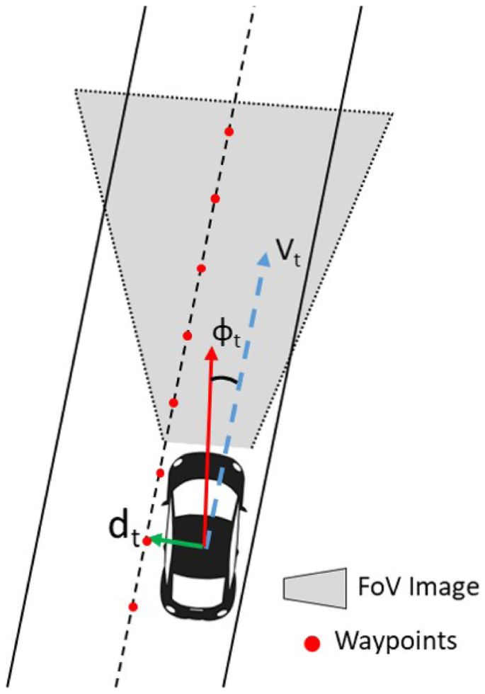

  

  State space definition

• b) Action space (A): To interact with the vehicle available in the simulator, the commands for throttle, steering and brake must be provided in a continuous way. Throttle and brake range is [0,1] and steering range is [-1,1]. Therefore, at each step the DRL agent must publish an action $(a_t)=(acc_t,steer_t,brake_t)$ with the commands into their ranges.

• c) State transition function ($P_a$) is the probability that action a in state s at time t will lead to state $s_{t+1}$ at time t+1. $P_a=P_r(s_{t+1}|s_t,a_t)$.

• d) Reward function $R(s_{t+1},s_t,a_t)$: This function generates the immediate reward of translating the agent from $s_t$ to $s_{t+1}$. The goal in a Markov decision process is to find a good “policy” $\pi (s)=a_t$ that will choose an action given a state. This function will maximize the expectation of cumulative future rewards and particularising the Eq. 8, we obtain:

  $$\begin{aligned} E = \sum _{t=0}^{\infty }\gamma ^t R(s_t,s_{t+1}) \end{aligned}$$

  (17)

4.2 Deep Q-Network Architecture

We have developed various agents that cover a wide variety of model architectures for the Deep Q-Network agents. Models will be first developed in simulation for safety reasons. Therefore, the agent will interact with CARLA and the code will be programmed in Python based on several open-source RL frameworks [49] (see Fig. 3) .

Fig. 3

DQN-based Deep Reinforcement Learning architecture

Following the previous formulation of the MDP, it is necessary to establish the general framework of what the developed DQN will be, clearly defining the actions and the reward that will come into play with the algorithm. The state vector depends on the data used as input for the DRL algorithm, which will be explained in later sections.

• a) Reward function. The proposed architecture obtains a driving features vector $df_t=(v_t,d_t,\phi _t)$ from the simulator. This vector is composed of the velocity of the vehicle in the direction of its heading $v_t$ , the distance to the center of the lane $d_t$ and the angle regarding the lane direction $\phi _t$. Considering that the objective is to go as fast as possible through the center of the lane without leaving the lane and avoiding collisions, the reward function must reward the longitudinal velocity and penalize the transverse velocity and divergence from the center of the lane. This approach is similar to the proposal made in [18] where TORCS (The Open Racing Car Simulator) is used. Variables involve in reward function are also shown in Fig. 2. Hereafter, we present the specific values assigned to R in a deterministic way.

  $$\begin{aligned} R=-200 \ \text {if collision or lane change or roadway departure} \end{aligned}$$

  (18)
  $$\begin{aligned} R = \sum _{t}|v_t cos\phi _t|-|v_t sin\phi _t|-|v_t||d_t| \ \text {if car in lane} \end{aligned}$$

  (19)
  $$\begin{aligned} R=100 \ \text {if goal position is reached} \end{aligned}$$

  (20)

• b) Control commands (Actions). CARLA needs control commands for steering [-1,1] and throttle [0,1]. Brake has not been implemented in this first version because the environment is free of obstacles and the regenerative braking of the vehicle is enough to stop the vehicle. The DQN policy allows generating discrete actions, so it is necessary to simplify the continuous control of actions to a discrete control. Taking this into account, the number of control commands has been simplified to a set of 27 discrete driving actions, discretizing steering angle and throttle position in an uniform way. Table 1 shows the set of control commands where there are 9 steering wheel positions and 3 throttle position.

  Table 1 Policy network. 27 classes

4.3 Deep deterministic policy gradient architecture

This section presents the basis structure of the DDPG architecture based on the previous algorithm explanation. This algorithm, as mentioned before, has two parts within it, the Actor and the Critic. This will be noticeable in the Fig. 4

Fig. 4

DDPG-based Deep Reinforcement Learning architecture

The system architecture based on DDPG algorithm, as can be seen, only change the Agent module in relation with DQN architecture. But additional modifications have been needed to assemble the whole system. In the same way as for the DQN, different models have been made to carry out a comparison among them. It has been done in the same way, by modifying the Agent and the data processing module to adapt the input data to the selected model in each case. Actions, reward and states should be established as well. For both the reward and the states, what was explained for the DQN algorithm can be applied, but the actions suffer an important change.

• a) Control commands (Actions). As difference with to DQN, this algorithm has a continuous character, so the actions do not have to be discrete in this case. Considering that the neural network outputs of the DRL algorithm is in the range [-1, 1] and that steering and throttle are in the range [-1, 1] and [0, 1] respectively, these outputs are directly mapped with the control commands. For the case of the throttle, an adjustment must be made to the ranges to match the ranges required by the simulator, but this is trivial.

5 Architecture proposals (agents)

This section describes the main work in this DRL project, the developed models for both Deep Q-Network and Deep Deterministic Policy Gradient will be explained in detail. Each model in this section has been implemented for both algorithms in the same way, so in following figures, a box representing both algorithms will be set and an internal switching will be done between them. For any of the two proposals, only the number of inputs of the first layer of the Net should be changed, which will depend on the data type taken as input from that network.

5.1 DRL-flatten-image agent

This agent uses a B/W segmented image of the road over the whole route that the vehicle must drive. This proposed agent reshapes the B/W frontal image, taken from the vehicle, from 640x480 pixels to 11x11, reducing the amount of data from 300k to 121. Once the image is resized, data is flatten and the state vector is formed with those 121 vector components. This vector is concatenated with the driving features vector and introduced to a really simple 2 Fully-Connected Layers network. (see Fig. 5).

$$\begin{aligned} S = ([P_{t0}, P_{t1}, P_{t2} ... P_{t120}], \phi _t, d_t) \end{aligned}$$

(21)

Fig. 5

DRL-Flatten-Image Agent

5.2 DRL-Carla-Waypoints agent

In this case, no image will be used to obtain the path to be followed by the agent. The waypoints will be received directly from the CARLA simulator, thanks to the available PythonAPI, (see Fig. 6). The process of obtaining these waypoints starts by calling the global planner (as explained above). This planner is given two points, initial and final, of a trajectory inside the map, and it returns a list of waypoints that links both points. The number of elements in this point list depends basically on how far apart the two points are from each other and how far apart the waypoints were defined at the beginning of the program.

Fig. 6

DRL-Carla-Waypoints Agent

These points are diretly referenced to the map, so passing these points to the DRL algorithm will be wrong. For example, for two straight road sections of the map, different waypoints will be set, but the vehicle should acting the same way for both trajectories, so it is impossible to obtain a good model with this approach. Waypoints are globally referenced to the point (0, 0, 0) on CARLA’s map. Therefore, they must be referenced to the ego_vehicle position. To do that, we apply the following transformation (rotation and translation) matrix and this local points are introduced as State vector S, where $[X_c, Y_c, Z_c]$ represents the current vehicle global position, and $\phi _c$ the current heading or yaw angle.

$$\begin{aligned} M = \begin{bmatrix} \cos {\alpha _c} &{} -\sin {\phi _c} &{} 0 &{} X_c \\ \sin {\alpha _c} &{} \cos {\phi _c} &{} 0 &{} Y_c\\ 0 &{} 0 &{} 1 &{} Z_c\\ 0 &{} 0 &{} 1 &{} 1\\ \end{bmatrix} \end{aligned}$$

(22)

A question to be solved is the size of the waypoints list taken into account that actions to be taken depend on car position and orientation and the near ahead section where the vehicle is driving. In an experimental way we fix a frame of 15 points. This list updates its content each step, and starts with the closest waypoint to the vehicle’s position, and is filled with the next 14 waypoints, working such as a FIFO (First In, First Out) along the episode. Likewise, for the image waypoints-based agent model, the $d_t$ and $\phi _t$ are added to form the state vector which is introduced directly into a double Fully-Connected network.

$$\begin{aligned} S = ([wp_{t0}...wp_{t14}], \phi _t, d_t) \end{aligned}$$

(23)

Each component of this waypoint list forming the State vector has coordinates (x, y). Although both options are provided in the program, the models are trained by entering only the x-coordinate of the points. This x-coordinate provides information on the lateral position of the waypoints with respect to the vehicle within the lane.

5.3 DRL-CNN agent

An step forward is trying to obtain road features from the ahead camera vehicle through a CNN as shown in Fig. 7, and from these features to determine the action to be taken by the vehicle in an end-to-end process and in online mode. To do this, two parts are proposed to set the State vector S, the first part extracts the road features through the CNN, and the second part is form by the same two Fully-Connected layers used in the previous cases. An RGB image as shown in Fig. 7, where the drivable area is highlighted, in the shape of [640x480] is used as input for CNN stage.

Fig. 7

DRL-CNN Agent

The CNN consist of three convolutional layers with 64 filters of size [7x7], [5x5] and [3x3] respectively, using all of them RELU as activation function and followed by an average polling layer. The output of this CNN is flattened and concatenated with driving features, and the whole state vector is used to fed 2-Fully-Connected layers which decided the final action to be taken.

Obviously, this agent model is more complex than the others, due to the nature of the state vector. The system will have much more difficulty to learn using a state vector as the one being considered, formed both by the road features extracted by the CNN and by the driving features.

$$\begin{aligned} S = ([I_t ],\phi _t,d_t) \end{aligned}$$

(24)

The total volume of data handle for this approach is quite a bit higher than for previous cases. For an image of 640x480 pixels, there would be 307200 data, which is 2500 times larger compared to the flatten-image-based model . This will lead to quite a few problems in the training process, which will be discussed later.

5.4 DRL-Pre-CNN agent

This case is quite similar to the previous one, except that now, the CNN is trained previously. This approach has been carried out because the model works well when waypoints are provided and much worse when features must be extracted, so the two options are mixed in this model. The option of training a network offline is considered, using a database of images and waypoints obtained directly from CARLA, in order to predict the waypoints from these images. This way, once the network has been trained, it will only have to be loaded into the main architecture and let it predict the waypoints at each step of the process, and enter these waypoints in the same way that in the previous cases to predict the action to be taken by the vehicle. Being concrete, once the Net is trained, it only will need the input image to obtain the corresponding waypoints. The difference with the previous CNN agent is observed in Fig. 8.

Fig. 8

DRL-Pre-CNN Agent

The network used to obtain the waypoints from the image is based on the developed by the group on a previous project [13]. Starting from this network, some substantial modifications have been carried out, such as the batch size, the size of intermediate layers, the elimination of some of the layers and the fitting of the sizes according to the images used and the outputs required.

In a broad sense an image is being used to predict the action to be taken, and the state vector could be:

$$\begin{aligned} S = ([I_t ],\phi _t,d_t) \end{aligned}$$

(25)

In reality the waypoints obtained from the pre-trained network are being used directly to feed the 2 Fully-Connected layers of the DRL so the state vector actually used, concatenating these points with the driving features, is as follows:

$$\begin{aligned} S = ([wp_{t0}...wp_{t14}], \phi _t, d_t) \end{aligned}$$

(26)

6 Results

The proposed approaches must be validated both individually and comparing among them. To carry out this validation process, a metric is defined in order to compare the error of each algorithm with respect to a ground truth provided by CARLA Simulator. In this way, the performance of the different approaches is compared following the same criteria.

Achieving a well-trained model from each proposed architecture for both algorithms (DQN, DDPG) is necessary, which are firstly obtained in the training stage. To achieve the trained models, a simple yet accurate training workflow is applied as follows:

• 1. Launch the simulator and iterate over M episodes and T steps for each episode.

• 2. At the beginning of the episode, call the A* based global planner to obtain the complete route from two random points on the map. Therefore, the training uses a different route in each episode.

• 3. At each episode, take an observation corresponding to the State S by concatenating the architecture-specific data entry D and the driving features vector. The State $S = ([D], \phi _t, d_t)$ is introduced to the DRL network which predicts the actions as output $A = (throttle, steering)$. Then, the predicted actions are sent to the simulator and the reward is calculated in function of this actuation.

• 4. The $lane\_invasor$ and $collision\_sensor$ are checked in each step. If any of these sensors are activated, the episode ends, and a new one is reset. This reset is done by relocating the vehicle in the centre of the lane, well oriented, and getting ready for the next route. If these sensors are not activated, the training process iterates over another new step.

• 5. The training stage finishes when the maximum number of episodes is reached.

Once the trained model are obtained, the error metric is applied. On the one hand, the training metrics are evaluated from the training episodes number needed to achieve the model. On the other hand, the error metric is carried out comparing the driven trajectories obtained by the trained models and an ideal route built by interpolating the waypoints provided by the CARLA’s A* based global planner. In addition, a classic method based on an LQR controller [20] is also evaluated using this method, thus being able to compare the AI-based controllers with one based on classic methodologies.

Both training stage and experimental results have been developed using a desktop PC (Intel Core i7-9700k, 32GB RAM) with CUDA-based NVIDIA GeForce RTX 2080 Ti 11GB VRAM.

6.1 DQN-DDPG performance comparison

In this section, the performance of the algorithms are compared both in training and validation stages, so at the end of this section, we will be able to discuss what algorithm relates to a better performance in a general way.

6.1.1 Training stage

In this subsection, the performance in training stage by each agent is presented. For this purpose, the total number of episodes used in training and the episode which registers the best performance, named as best episode, are used. The best episode choice is obtained considering the total accumulated reward value at the end of the episode, as well as the maximum distance driven in the episode. The model obtained in this best episode is the one to be used in the validation stage. The training process necessary to reach a trained model is carried out as was explained in the previous section.

Table 2 summarizes the results obtained for the two algorithms at this stage. These results from each algorithm do not demonstrate much by themselves, but differences are remarkable among them, translating them into longer or shorter training time. The difference between the performance of the DQN and the DDPG is that the first algorithm needs at least 8300 episodes to obtain a good model in one of the proposed agents, while the second one is able of doing it using only 50 episodes. This fact implies a drastic training time reduction. DQN obtains best results as the episodes increases, whereas DDPG reach the best models in early episodes, and this is the reason why the maximum number of training episodes is larger in DQN. DQN needs more episodes for training due to its learning process uses a decay parameter in the reward sequence.

Table 2 Training performance metrics for DQN & DDPG

6.1.2 Validation stage

This subsection presents the quantitative results obtained using the trained models. In order to compare both algorithms well, a certain route is selected on the map and each agent is driven along it. Each agent drives on this track over 20 iterations, thus calculating the RMSE from the real route and an ideal route obtained by interpolating the waypoints, as describes [20]. In the same way is obtained the RMSE produced by the classic control method and the simulator manual control mode driven by a random user.

The chosen route is shown in Fig. 9 and is driven by each agent for both algorithms, being completed at each attempt. This stretch of road has curves in both directions and straight sections, which is quite convenient for testing this kind of algorithms, having a route distance of approximately 180 meters, and belonging to CARLA map named “Town01”. Table 3 shows the RMSE generating when the agent navigates the route 20 times. In addition, the maximum error on the route, and the average time spent in getting from the starting to the end point are shown too.

Fig. 9

Evaluation trajectory for DQN & DDPG

Table 3 Validation metrics for DQN & DDPG

Improving the performance of a classic controller is not an easy task, so the results shown in the table must be put into perspective, due to an AI based controller for AV is an innovative research line. Both the DQN and the DDPG obtain good results when driving the trajectories. Although none of the agents presented is able to improve the performance of the LQR-based controller, the DDPG is quite close. The results can be considered qualitatively similar to others published in the literature [8, 48].

This table also shows the notorious difference in validation performance of the DDPG with respect to the DQN.

One of the main drawbacks using DQN is its discrete nature (discrete actions for controlling speed and steer). This provokes that driving is much more complex and training requires more time and worse results are obtained.

Considering the better performance of DDPG we will focus on this strategy, having in mind that our final goal is the implementation of the navigation architecture in the real vehicle [1]. Therefore, in the following section, architecture based in DDPG algorithm, which is more stable and reliable, is testing in some new routes.

6.2 DDPG performance in validation stage

This section focuses only on the DDPG algorithm due to the results obtained in the previous comparison. To validate the architecture based on DDPG, 20 different routes, with a range between [180, 700] meters, are driven by each agent, obtaining the same metrics discussed above based on the MRSE. The results shown are calculated from the mean of the 20 routes driven. In this case the whole routes are also completed on each attempt.

Table 4 confirms the fact presented in previous section, related to the difficulty of improving the classic controllers performance, but following the same line, the DDPG performs trajectories very similar to the LQR control method. It is observed how our approaches are able to complete the specified routes in a way that is practically identical to the LQR controller, getting the best performance with Carla-Waypoints based agent. As can also see in the table, the approach based on Carla-Waypoints achieves the best results in relation with our proposals, although Pre-CNN and Flatten-Image approaches are also very close.

Table 4 Validation metrics for DDPG

To complete this section, some qualitative results are presented in two of the paths performed, comparing the trajectory followed by each controller.

As we can see in Fig. 10 two routes are established within the “Town01” of CARLA, and the trained models are driven over these routes recording trajectory while navigate. In order to compare their performance, the path recorded by the LQR and the one obtained by the ground truth are also included. All the agents are able to follow the path in a proper way. Although some do it in a better way than others, all of them completes the defined route.

Fig. 10

Qualitative results by trajectories comparison

Comparing the agents with lower RMSE than those obtained when using a classic control method, a difference of between 4 and 7 centimetres are found, distances that in relation to the width of any lane are practically irrelevant, as well as at the driving time. The advantage of the robustness and reliability of the classic control methods is offset by the difficulty of tuning these controllers, unlike if Deep Learning methods are used to, which are fully reproducible by anyone in any environment without making major changes, and which is more important, without having a specific knowledge of electronic control theory.

7 Conclusions

In this paper, an approach for autonomous driving navigation based on Deep Reinforcement Learning algorithms is shown, by using CARLA Simulator in order to both train and evaluate. After countless tests, a robust structure for the training of these algorithms has been carried out, being able to implement both Deep Q-Network and Deep Deterministic Policy Gradient algorithms.

The results reported in this work show how it is possible to treat the paradigm of navigation in autonomous vehicles using new techniques based on Deep Learning. Both DQN and DDPG are capable of reaching the goal by driving the trajectory, although DDPG obtain better performance and driving is more similar to that performed by a human driver since it implements continuous control in both speed and steering. We hope that our proposed architecture based on DRL control layer, will serve as a solid baseline in the state-of-the art of Autonomous Vehicles navigation tested in realistic simulated environments.

8 Future works

As future work, we are working on implementing the DDPG-based control into our autonomous vehicle. Currently we have implemented the CARLA-waypoints Agent because it is the most similar to the one available in the real vehicle since the mapping and planning modules obtain the same data provided by CARLA (waypoints), but in the future the goal is to use the perception system based on camera and lidar. The main drawbacks that we are going to tackle are modelling the real environment to obtain a precise map to train in CARLA and to incorporate ROS in the system because the proposed architecture has to work properly both in simulation and real.

References

Arango JF, Bergasa LM, Revenga PA, Barea R, López-Guillén E, Gómez-Huélamo C, Araluce J, Gutiérrez R (2020) Drive-by-wire development process based on ros for an autonomous electric vehicle. Sensors 20(21):6121
Barea R, Pérez C, Bergasa LM, López-Guillén E, Romera E, Molinos E, Ocana M, López J (2018) Vehicle detection and localization using 3d lidar point cloud and image semantic segmentation. In: 2018 21st International Conference on Intelligent Transportation Systems (ITSC). IEEE, pp 3481–3486
Bemporad A, Morari M, Dua V, Pistikopoulos EN (2002) The explicit linear quadratic regulator for constrained systems. Automatica 38(1):3–20
Byrne R, Abdallah C (1995) Design of a model reference adaptive controller for vehicle road following. Math Comput Model 22(4–7):343–354
Chan CY (2017) Advancements, prospects, and impacts of automated driving systems. Int J Transp Sci Technol 6(3):208–216
Cheein FAA, De La Cruz C, Bastos TF, Carelli R (2010) Slam-based cross-a-door solution approach for a robotic wheelchair. Int J Adv Robot Syst 155–164
Chen J, Yuan B, Tomizuka M (2019) Deep imitation learning for autonomous driving in generic urban scenarios with enhanced safety. arXiv preprint arXiv:1903.00640
Chen L, Hu X, Tang B, Cheng Y (2020) Conditional DQN-based motion planning with fuzzy logic for autonomous driving. IEEE Trans Intell Transp Syst
Choomuang R, Afzulpurkar N (2005) Hybrid kalman filter/fuzzy logic based position control of autonomous mobile robot. Int J Adv Robot Syst 2(3):20
Codevilla F, Miiller M, López A, Koltun V, Dosovitskiy A (2018) End-to-end driving via conditional imitation learning. In: 2018 IEEE International Conference on Robotics and Automation (ICRA). IEEE, pp 1–9
Coulter RC (1992) Implementation of the pure pursuit path tracking algorithm. Tech. rep., Carnegie-Mellon UNIV Pittsburgh PA Robotics INST
De Bruin T, Kober J, Tuyls K, Babuška R (2015) The importance of experience replay database composition in deep reinforcement learning. In: Deep reinforcement learning workshop, NIPS
del Egido J, Bergasa LM, Romera E, Huélamo CG, Araluce J, Barea R (2018) Self-driving a car in simulation through a CNN. In: Workshop of Physical Agents. Springer, pp 31–43
Dosovitskiy A, Ros G, Codevilla F, Lopez A, Koltun V (2017) Carla: An open urban driving simulator. arXiv preprint arXiv:1711.03938
Duan Y, Chen X, Houthooft R, Schulman J, Abbeel P (2016) Benchmarking deep reinforcement learning for continuous control. In: International Conference on Machine Learning. pp 1329–1338
Dupuis M, Strobl M, Grezlikowski H (2010) Opendrive 2010 and beyond–status and future of the de facto standard for the description of road networks. In: Proc. of the Driving Simulation Conference Europe. pp 231–242
Fan J, Wang Z, Xie Y, Yang Z (2020) A theoretical analysis of deep Q-learning. In: Learning for Dynamics and Control. PMLR, pp 486–489
Ganesh A, Charalel J, Sarma MD, Xu N (2016) Deep reinforcement learning for simulated autonomous driving
Geiger A, Lenz P, Urtasun R (2012) Are we ready for autonomous driving? the Kitti vision benchmark suite. In: 2012 IEEE Conference on Computer Vision and Pattern Recognition. IEEE, pp 3354–3361
Gutiérrez R, López-Guillén E, Bergasa LM, Barea R, Pérez Ó, Gómez-Huélamo C, Arango F, Del Egido J, López-Fernández J (2020) A waypoint tracking controller for autonomous road vehicles using ros framework. Sensors 20(14):4062
Hessburg T, Tomizuka M (1994) Fuzzy logic control for lateral vehicle guidance. IEEE Control Syst Mag 14(4):55–63
Hou Y, Liu L, Wei Q, Xu X, Chen C (2017) A novel DDPG method with prioritized experience replay. In: 2017 IEEE International Conference on Systems, Man, and Cybernetics (SMC). IEEE, pp 316–321
Kendall A, Hawke J, Janz D, Mazur P, Reda D, Allen JM, Lam VD, Bewley A, Shah A (2019) Learning to drive in a day. In: 2019 International Conference on Robotics and Automation (ICRA). IEEE, pp 8248–8254
Le-Anh T, De Koster M (2006) A review of design and control of automated guided vehicle systems. Eur J Oper Res 171(1):1–23
Lenain R, Thuilot B, Cariou C, Martinet P (2005) Model predictive control for vehicle guidance in presence of sliding: Application to farm vehicles path tracking. In: Proceedings of the 2005 IEEE international conference on robotics and automation. IEEE, pp 885–890
Liang M, Yang B, Wang S, Urtasun R (2018) Deep continuous fusion for multi-sensor 3d object detection. In: Proceedings of the European Conference on Computer Vision (ECCV). pp 641–656
Liang X, Wang T, Yang L, Xing E (2018) Cirl: Controllable imitative reinforcement learning for vision-based self-driving. In: Proceedings of the European Conference on Computer Vision (ECCV). pp 584–599
Lillicrap TP, Hunt JJ, Pritzel A, Heess N, Erez T, Tassa Y, Silver D, Wierstra D (2015) Continuous control with deep reinforcement learning. arXiv preprint arXiv:1509.02971
Lin LJ (1992) Reinforcement learning for robots using neural networks (phd thesis)
Luo Y, Chen Y (2009) Fractional order [proportional derivative] controller for a class of fractional order systems. Automatica 45(10):2446–2450
Mao H, Alizadeh M, Menache I, Kandula S (2016) Resource management with deep reinforcement learning. In: Proceedings of the 15th ACM Workshop on Hot Topics in Networks. pp 50–56
Martín UI et al (2018) Generación de trayectorias robóticas mediante aprendizaje profundo por refuerzo. Master’s thesis, Universitat Politècnica de Catalunya
Matt V, Aran N (2017) Deep reinforcement learning approach to autonomous driving
Mnih V, Kavukcuoglu K, Silver D, Graves A, Antonoglou I, Wierstra D, Riedmiller M (2013) Playing Atari with deep reinforcement learning. arXiv preprint arXiv:1312.5602
Mnih V, Kavukcuoglu K, Silver D, Rusu AA, Veness J, Bellemare MG, Graves A, Riedmiller M, Fidjeland AK, Ostrovski G et al (2015) Human-level control through deep reinforcement learning. Nature 518(7540):529–533
Montemerlo M, Becker J, Bhat S, Dahlkamp H, Dolgov D, Ettinger S, Haehnel D, Hilden T, Hoffmann G, Huhnke B et al (2008) Junior: The stanford entry in the urban challenge. J Field Rob 25(9):569–597
Pérez-Gil Ó, Barea R, López-Guillén E, Bergasa LM, Revenga PA, Gutiérrez R, Díaz A (2020) DQN-based deep reinforcement learning for autonomous driving. In: Workshop of Physical Agents. Springer, pp 60–76
Raimondi FM, Melluso M (2005) A new fuzzy robust dynamic controller for autonomous vehicles with nonholonomic constraints. Robot Auton Syst 52(2–3):115–131
Sáez Á, Bergasa LM, López-Guillén E, Romera E, Tradacete M, Gómez-Huélamo C, del Egido J (2019) Real-time semantic segmentation for fisheye urban driving images based on erfnet. Sensors 19(3):503
Sanders A (2016) An introduction to unreal engine 4. AK Peters/CRC Press
Sasaki H, Horiuchi T, Kato S (2017) A study on vision-based mobile robot learning by deep q-network. In: 2017 56th Annual Conference of the Society of Instrument and Control Engineers of Japan (SICE). IEEE, pp 799–804
Silver D, Hubert T, Schrittwieser J, Antonoglou I, Lai M, Guez A, Lanctot M, Sifre L, Kumaran D, Graepel T et al (2017) Mastering chess and shogi by self-play with a general reinforcement learning algorithm. arXiv preprint arXiv:1712.01815
Urmson C, Anhalt J, Bagnell D, Baker C, Bittner R, Clark M, Dolan J, Duggins D, Galatali T, Geyer C et al (2008) Autonomous driving in urban environments: Boss and the urban challenge. J Field Rob 25(8):425–466
Wang FY (2017) Ai and intelligent vehicles future challenge (IVFC) in China: From cognitive intelligence to parallel intelligence. In: 2017 ITU Kaleidoscope: Challenges for a Data-Driven Society (ITU K). IEEE, pp 1–2
Wang S, Jia D, Weng X (2018) Deep reinforcement learning for autonomous driving. arXiv preprint arXiv:1811.11329
Wang W, Nonami K, Ohira Y (2008) Model reference sliding mode control of small helicopter XRB based on vision. Int J Adv Robot Syst 5(3):26
Xiong X, Wang J, Zhang F, Li K (2016) Combining deep reinforcement learning and safety based control for autonomous driving. arXiv preprint arXiv:1612.00147
Ye F, Zhang S, Wang P, Chan CY (2021) A survey of deep reinforcement learning algorithms for motion planning and control of autonomous vehicles. arXiv preprint arXiv:2105.14218
Yurtsever E, Capito L, Redmill K, Ozguner U (2020) Integrating deep reinforcement learning with model-based path planners for automated driving. arXiv preprint arXiv:2002.00434
Zhang F, Li J, Li Z (2020) A td3-based multi-agent deep reinforcement learning method in mixed cooperation-competition environment. Neurocomputing 411:206–215
Zhao J, Ye C, Wu Y, Guan L, Cai L, Sun L, Yang T, He X, Li J, Ding Y, et al (2018) Tiev: The tongji intelligent electric vehicle in the intelligent vehicle future challenge of China. In: 2018 21st International Conference on Intelligent Transportation Systems (ITSC). IEEE, pp 1303–1309
Zhuang D, Yu F, Lin Y (2007) The vehicle directional control based on fractional order pd^ m^ u controller. Journal-Shanghai Jiaotong University-Chinese Edition 41(2):0278
Funding
Open Access funding provided thanks to the CRUE-CSIC agreement with Springer Nature. This work has been funded in part from the Spanish MICINN/FEDER through the Techs4AgeCar project (RTI2018-099263-B-C21) and from the RoboCity2030-DIH-CM project (P2018/NMT- 4331), funded by Programas de actividades I+D (CAM) and cofunded by EU Structural Funds.
Author information
Authors and Affiliations
Corresponding author
Additional information
Publisher’s Note
Springer Nature remains neutral with regard to jurisdictional claims in published maps and institutional affiliations.
Rights and permissions
Open Access This article is licensed under a Creative Commons Attribution 4.0 International License, which permits use, sharing, adaptation, distribution and reproduction in any medium or format, as long as you give appropriate credit to the original author(s) and the source, provide a link to the Creative Commons licence, and indicate if changes were made. The images or other third party material in this article are included in the article's Creative Commons licence, unless indicated otherwise in a credit line to the material. If material is not included in the article's Creative Commons licence and your intended use is not permitted by statutory regulation or exceeds the permitted use, you will need to obtain permission directly from the copyright holder. To view a copy of this licence, visit http://creativecommons.org/licenses/by/4.0/.
About this article
Cite this article
Pérez-Gil, Ó., Barea, R., López-Guillén, E. et al. Deep reinforcement learning based control for Autonomous Vehicles in CARLA. Multimed Tools Appl 81, 3553–3576 (2022). https://doi.org/10.1007/s11042-021-11437-3
Received:
Revised:
Accepted:
Published:
Issue Date:
DOI: https://doi.org/10.1007/s11042-021-11437-3