Machine learning method for cosmetic product recognition: a visual searching approach

Abstract

A cosmetic product recognition system is proposed in this paper. For this recognition system, we have proposed a cosmetic product database that contains image samples of forty different cosmetic items. The purpose of this recognition system is to recognize Cosmetic products with there types, brands and retailers such that to analyze a customer experience what kind of products and brands they need. This system has various applications in such as brand recognition, product recognition and also the availability of the products to the vendors. The implementation of the proposed system is divided into three components: preprocessing, feature extraction and classification. During preprocessing we have scaled and transformed the color images into gray-scaled images to speed up the process. During feature extraction, several different feature representation schemes: transformed, structural and statistical texture analysis approaches have been employed and investigated by employing the global and local feature representation schemes. Various machine learning supervised classification methods such as Logistic Regression, Linear Support Vector Machine, Adaptive k-Nearest Neighbor, Artificial Neural Network and Decision Tree classifiers have been employed to perform the classification tasks. Apart from this, we have also performed some data analytic tasks for Brand Recognition as well as Retailer Recognition and for these experimentation, we have employed some datasets from the ‘Kaggle’ website and have obtained the performance due to the above-mentioned classifiers. Finally, the performance of the cosmetic product recognition system, Brand Recognition and Retailer Recognition have been aggregated for the customer decision process in the form of the state-of-the-art for the proposed system.

1 Introduction

In real-world applications, E-commerce plays an important role in the field of commercial online transactions to increase the buying and selling of products through the Internet. These applications are maintained by E-commerce and E-business sometimes used interchangeable [19]. Generally, E-commerce involves five steps: (a) Problem recognition, (b) Information search, (c) Alternative solution evaluation, (d) Purchase decision and (e) Pre-purchase and Post-purchase decision during the consumer decision process. Problem recognition is the step to recognize the need for a service or a product and it is driven by both internal and external stimuli such that a consumer can recognize his/her wants. This recognition needs the information to understand how the product will fulfill his/her requirements. This information is obtained through the search of the consumer decision information system. Finally, the selected information undergo for evaluating the pre-purchase and post-purchase (https://econsultancy.com/blog/69460-image-recognition-in-ecommerce-visual-search-product-tagging-and-content-curationhttps://econsultancy.com/blog/69460-image-recognition-in-ecommerce-visual-search-product-tagging-and-content-curation) decisions. This field of online marketing for product selection based on image recognition has been increased for productivity and marketing in E-commerce.

Image processing [6] pertains to the alteration and analysis of pictorial information and the common case of an image processing is to enhance the image until its subjective appearing to us is most appealing. Nowadays the problems like product recognition/classification for commercial online transactions are more demanding and these are solved by image processing and machine learning algorithms. The machine learning [32] applications belong to the artificial intelligence systems which have the ability to learn and to improve the system from the experiences without being explicitly programmed. Its applications focus on the development of computer programs that can access data and use it to learn for themselves.

Computer vision [15] is a field of research in computer science that provides processing, analyzing, identifying and enhancing the images and videos in the same way that human vision does with appropriate output. The computer vision gives the facilities to interpret what the computer sees and it acts the matters accordingly. In E-commerce the combined applications of computer vision and machine learning give the various facilities to the content curation & product tagging applications for visual search problems [23].

Visual search is a kind of perceptual task that requires attention for involving a visual environment for a particular product among the various products (https://econsultancy.com/blog/69460-image-recognition-in-ecommerce-visual-search-product-tagging-and-content-curationhttps://econsultancy.com/blog/69460-image-recognition-in-ecommerce-visual-search-product-tagging-and-content-curationhttps://econsultancy.com/blog/69460-image-recognition-in-ecommerce-visual-search-product-tagging-and-content-curation). It is capable to locate an object from a collection of complex objects. Product tagging is the descriptors assigned to the specific products to organize, document and track their progress. It contains a phrase corresponding to each ordered product. Content curation is the process of gathering information relevant to a particular topic or area of interest. It is used for businesses as well as end users (https://www.lucidchart.com/blog/consumer-decision-making-process).

The image recognition in E-commerce based business [50], facilitates the individual business brand with a reputation for value with honesty, wining with retaining and a wealthy market share to the customer. Moreover, the factors from social networks such as likes, tags, comments about a product by the customers also increase the advantages of image recognition in E-commerce based business. Sometimes recognizing the customer emotions e.g. facial expressions during the consumer decision process also revolutionizes online marketing in E-commerce based business [43].

In object recognition [28], a specific object is identified in a digital image or video. This object recognition has immense applications in the field of object localization, obstacle detection, scene understanding, texture classification, medical analysis, monitoring and surveillance, biometric and navigation, etc. Generally, the object recognition problems are categorized into two broad categories: (a) instance-based recognition and (b) class-based recognition [55]. Instance recognition relates to recognizing the 2D or 3D rigid objects with different viewpoints, cluttered background with occlusions conditions. These problems are more mature and being used in various commercial applications such as generic class recognition, photosynthesis based applications, etc. Class recognition problems involve the recognizing of a particular class such as Car, Chair, Air-plane, Bicycle, etc., and this type of recognition problem is much challenging for state-of-the-art computer vision research problems [42].

The appearance of an object in the object recognition task can be varied due to the scene clutter, photometric effects, changes in shape and viewpoints. The novelty of object recognition task lies on the invariant to viewpoint changes, object transformations, robust to noise and occlusion. These are performed by analyzing textures in the image or video frames. The texture is collection of texel elements arranges in regular or non-regular patterns which are calculated during feature computation design to quantify the information about the spatial arrangement of colors or intensities in the image [38] and further we analyze these textures and obtain the features which are intended to be non-redundant, informative, discriminative, reduced in dimensionality and leading to better human interpretation system [32].

Rothganger et al. [46] had used local affine-invariant image descriptors and multi-view spatial constraints for modeling 3D objects and recognizing the objects. Obdržálek & Matas [36] had obtained the maximally stable extrem regions based on the computation of affine-invariant local frames and tentative region-to-region correspondences. Felzenszwalb & Huttenlocher [13] had represented a generic object recognition problem by arranging the deformation configuration handled by spring-like connections between pairs of parts.

Fergus et al. [14] had proposed weakly supervised scale-invariant learning models for visual object recognition. Sivic & Zisserman [54] had proposed an approach for object retrieval system that searches and localizes all of the occurrences of an object in a video by introducing a set of viewpoint invariant region descriptors such that the recognition can proceed successfully in the unconstrained environment with varying viewpoints, illumination, and occlusions. Sivic [53] had built a hierarchical structure for the visual world objects from a collection of unlabeled images that follows a multi-layer hierarchy tree that performs the visual search of object classification and object detection tasks.

Piccinini et al. [41] had presented an approach for detecting and localizing the duplicated objects in pick-and-place applications under occlusion conditions using SIFT descriptors followed by clustering methods. Tokarczy et al. [57] had proposed a boosting classifier using the optimal features from a Randomized Quasi-Exhaustive set features extracted from the remote sensing images.

A deformable deep convolutional neural networks (CNN) for generic object detection had been built [40] where a deformation constrained pooling layer with geometric constraint and penalty was introduced. Liang & Hu [27] had employed a recurrent CNN (RCNN) architecture by incorporating the recurrent connections into every convolutional layer, which enhances the ability of the RCNN model to integrate the context information for the object recognition tasks. Xu et al. [62] had proposed a model using the ImageNet database to conduct the few-shot object recognition task which works on machine labeled annotated images with some novel categorical object databases. Chan et al. [7] had built a binary integrated descriptor that had various invariant properties such as rotation, scale and polarity of edges through the unique binary logical operated encoding and matching techniques for texture-less object databases. The integrated part based representations had been introduced into convolutional neural networks that result in rotational and translational invariant features for recognizing the different birds [51]. Hence, the contributions of this work are as follows:

• An E-commerce based application for commercial online transactions for the buying and selling of cosmetic products through the Internet has been proposed in this paper.

• Both image-based and text-based information have been considered during implementation of the proposed system and for this various computer vision algorithms and machine learning techniques have been employed and investigated to build the proposed system.

• For the image-based information, a cosmetic product database has been proposed that contains image samples of forty different cosmetic items and using this dataset the cosmetic product recognition system has been proposed which can identify the type of cosmetic product based on an input image by the customer. The implementation of this recognition system has been divided into three components: image preprocessing, feature extraction and classification.

• For the text-based information, the data analytic tasks have been performed for two recognition systems: (i) Brand Recognition and (ii) Retailer Recognition. For both of these recognition systems, the data preprocessing, feature analysis and classification tasks have been performed and have obtained the predictive model individually for predicting the brand strategies and the retailer business strategies. For data analytic tasks, the datasets are downloaded from the ‘Kaggle’ website.

• Finally, the outcomes from the cosmetic product recognition system, Brand Recognition system, and Retailer Recognition system have been aggregated to derive the prediction for the Customer Decision Process through visual search techniques.

The organization of this paper is as follows: Section 2 gives the detailed description about the proposed system. Experimental results and discussions have been reported in Section 3. Section 4 concludes this paper.

2 Proposed method

Cosmetic products are very important in our daily life for the improvement of living standards. Cosmetics products are used to enhance or alter the appearance or fragrance of the body and it is due to the bringing of these products by the potential customers. Among the various cosmetics products, many of them are used for applying to the face and hair. These products are generally mixtures of chemical compounds i.e. some being derived from natural sources and some being synthetics. The commonly used of these cosmetics include lipstick, mascara, eye-shadow, foundation, rouge, skin-cleansers, skin-lotions, shampoo, hair-styling products (i.e. gel, hair-spray, etc.), perfume and cologne. Cosmetic products that are applied to the face to enhance their appearance are often called makeup. In this work, we capture the images of these cosmetic products and proposed a system for recognizing these products by applying the computer vision algorithms and applications. As stated earlier that these applications have been employed to recognize the different brands and their corresponding retailers such that the customer can analyze the kind of products and the brands that they need. Hence during recognizing cosmetic products by images, while we are also recognizing their brands as well as retailers. During implementation, we divide the proposed system into three components: (i) preprocessing, (ii) features extraction and (iii) classification. The block diagram of the proposed system is shown in Fig. 1.

Fig. 1

Block diagram of the proposed system

2.1 Cosmetic product recognition

2.1.1 Image preprocessing

During image preprocessing, we have transformed the color image of a cosmetic product to its gray-scaled to speed up the process. The grayscale image has been represented by its luminance property i.e. pixel value using 8 bits representation while each pixel ranges from 0 to 255. This transformation of the color image to the grayscaled image may lose contrast, shadow, sharpness, and structure of some relevant texture but still, we accept these challenges and we have employed the grayscaled images [49]. Here any extra algorithms for background removal, noise filtering and region of interest for the required object, have not been performed. The images are captured at unconstrained environments with distinct background details, illumination variations, scale invariants within the intra-class images. Fig. 2 shows some examples of preprocessed images employed in the proposed system.

Fig. 2

Preprocessed images for the cosmetic product recognition system

2.1.2 Feature Extraction

The images after preprocessing undergo for feature computation task. To extract useful information in terms of numerical values from an image is called features. During feature extraction, we extract more distinctive and discriminating information from an image such that there will be low variation between intra-class (similar) images while the high variation between inter-class (dissimilar) images. The extraction of those kinds of features is more challenging for state-of-the-art computer vision problems such as object recognition, texture classification, Biometric recognition, region segmentation, etc. The advantages of these features are that these are difficult to understand, uncorrelated by human and reduction in dimensionality. During the implementation of these features mainly two different feature representation approaches have been considered such as (i) global feature representation (say $\mathcal {F}_{G}$) and local feature representation (say $\mathcal {F}_{L}$) schemes.

• Global features [58] ($\mathcal {F}_{G}$) describe the image I as a whole and is the representation of the entire image (Fig. 3(a)). In some applications such as image retrieval, object classification, object detection, the global feature representation scheme has been employed.

  Fig. 3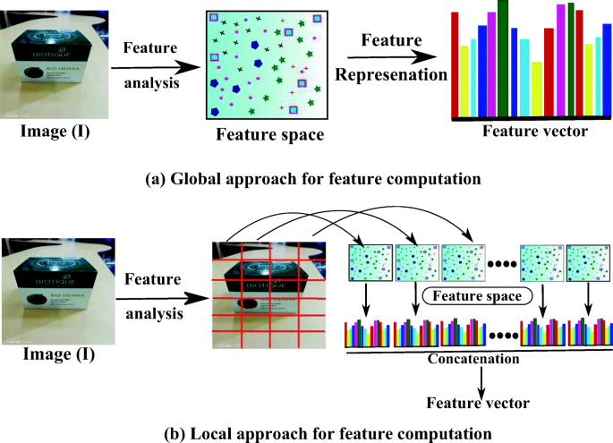

  

  a Global feature representation scheme ($\mathcal {F}_{G}$) and b Local feature representation scheme ($\mathcal {F}_{L}$) from the image I

• During the local feature representation scheme [58], the image I is partitioned into several blocks or patches w s of size n × n. Then from each patch w, the textures are analyzed and compute some features f_w. The features from each w are concatenated to obtain its global representation $\mathcal {F}_{L}=[f_{w_{1}},\cdots ,f_{w_{M}}]$ (M be the total number of patches extracted from I). Fig. 3(b) demonstrates an example of local feature representation scheme. This scheme is being widely used in various computer vision problems such for instance based dichotomy model for object recognition, class or categorical based object recognition.

The images from the above pre-processing steps contain a set of divergent and competent features to characterize the texture patterns in that image [12]. There exist several methods for texture analysis [20] such as (i) transformed-based, (ii) structural-based and (iii) statistical-based texture analysis approaches which are widely used in practice. The transformed-based approaches are related to statistics of filter responses such as wavelets, Gabor, Contourlet and radon transform. Structural-based approaches relate with the geometrical representation of the texture elements which are characterized by texture primitives or texture elements, and the spatial arrangement of these primitives. Mathematical morphology, Local Binary Pattern, and Fractal Dimension methods are under this category. The statistical-based approach relates to the local properties of texture and the texture features computed on the statistical distribution of image intensities over a region in the image. Grey-level co-occurrence matrix, Eigen region, Textural Edgeness descriptor, and their variants are under this category. Texture features under transformed, structural and statistical-based approaches are discussed below.

• 1. Transformed based approaches

  • DCT:- It stands for discrete cosine transform [3] and it transforms the image I from the spatial to the frequency domain. DCT divides I into several spectral sub-bands of differing importance concerning the quality of the image and obtains the DCT coefficient globally from I and then these coefficients are analyzed to obtain $\mathcal {F}_{G}^{DCT}\in \mathbb {R}^{T_{1}}$ features for I.

  • DFT:- It stands for Discrete Fourier Transform [18] and is equivalent to the continuous Fourier transformation. DFT is applied on I to extract the spectral information that takes over the whole I to obtain $\mathcal {F}_{G}^{DFT} \in \mathbb {R}^{T_{2}}$ features for I.

  • Gabor Filter:- It is bandpass filters used to estimate the depth information from I and is performed by multiplying a Gaussian envelope function with a complex oscillation that results in the impulse response of these filters [5]. Here each of the filter masks with 6 scales and 8 orientations is convolved with I and obtain magnitude, gradient and histogram information from each convolved image to compute the feature vector $\mathcal {F}_{G}^{Gabor}\in \mathbb {R}^{T_{3}}$.

  • Wavelets:- Wavelets are based on small waves that are employed to perform the multi-resolution processing for analyzing the texture patterns in I [5, 59]. Here Discrete Meyer wavelets have been applied on I and obtain the corresponding low, horizontal, vertical and diagonal details at different levels and compute features $\mathcal {F}_{G}^{Wave}\in \mathbb {R}^{T_{4}}$ globally over I.

• 2. Structural based approaches

  • Gradient Feature:- The image gradient [60] is the change of direction of intensities in the image I. It is a two-variable function computed at each pixel by the derivatives in horizontal and vertical directions in such a way that the gradient vector points to the largest possible direction of increasing intensities and its length corresponds to the rate of change in that direction. Here both first and second-order gradient statistics are computed from each patch w to compute features locally and finally concatenate those features to obtain $\mathcal {F}_{L}^{Grad} \in \mathbb {R}^{\mathcal {S}_{1}}$ feature vector from I.

  • Fractal dimension:- It is used for characterizing fractal patterns in the image I by quantifying the complexity as a ratio of change in detail to the change in scale for that image region. There are several types of fractal dimension have been employed, among them, Box-counting, Differential Box-Counting and Triangular Pyramid based methods are widely used [25] [9]. Here also the image I is partitioned into several patches and from each patch w, the fractal features are extracted locally and finally, concatenate these features to obtain the feature vector $\mathcal {F}_{L}^{Fractal} \in \mathbb {R}^{\mathcal {S}_{2}}$ for I.

  • Mathematical Morphologic:- The multi-scale mathematical morphological (MM) based features play an important role to analyze textures in I. MM is a powerful tool provides top-hat transformation which is the combination of bright and dark top-hat transformation. Here top-hat transformation is being applied on each patch w and compute mean, standard deviation and moments features. Then features extracted from each w are concatenated to obtain the feature vector $\mathcal {F}_{L}^{Morph} \in \mathbb {R}^{\mathcal {S}_{3}}$ for I.

  • CCA:- It stands for connected components analysis to obtain groups of pixels called components based on pixel connectivity. The extraction and labeling of such disjoint connected components extracted from each patch w of I are used to compute features such as number of connected components, connectivity, statistical measures, extrema points detection etc. The concatenation of these features from all patches are used to obtain the feature vector $\mathcal {F}_{L}^{CCA} \in \mathbb {R}^{\mathcal {S}_{4}}$ for I.

  • MSER:- It stands for maximally stable extremal regions which is used for blob detection from an image I [30]. It works based on computation of comprehensive numbers from the corresponding images to perform better stereo matching and object recognition tasks. Here from each patch w, MSER features are computed and have been concatenated these features from all the patches to obtain $\mathcal {F}_{L}^{MSER} \in \mathbb {R}^{\mathcal {S}_{5}}$ feature vector for I.

• 3. Statistical based approaches

  • LBP:- Local binary patterns (LBP) is a type of visual descriptor used for feature computation from I [21, 37]. It operates on the pixels thresholding at 3 × 3 neighborhood of each pixel and obtains an eight-digit binary number which is converted to decimal for convenience. These decimals are used to obtain the histogram. Here the histogram is obtained from each patch w and then accumulates these histograms from corresponding patches to obtain $\mathcal {F}_{L}^{LBP} \in \mathbb {R}^{S_{1}}$ feature vector for I.

  • HOG:- The histogram of oriented gradients (HOG) [10] is a feature descriptor used in object detection, region segmentation and person identification [31] problems. HOG counts occurrences of gradient orientation with the specified histogram bins computed from localized portions of I [16]. It is similar to the edge orientation histograms, scale-invariant feature transform descriptors, and shape contexts [10]. To extract HOG descriptors, the image I is partitioned into different patches and extracting HOG descriptors from each patch w, and concatenate these descriptors to obtain $\mathcal {F}_{L}^{HoG} \in \mathbb {R}^{S_{2}}$ feature vector for I.

  • SIFT:- Scale-Invariant Feature Transform (SIFT) [29] is used to extract features which have geometric invariant properties (like translation, rotation, scaling) to illumination changes in different viewpoint conditions. To compute SIFT features from I, several Gaussian filtered images are generated at different scales and then the difference of Gaussian (DoG) images is obtained from the neighborhoods of each scale. The DoG images are used to detect extrema points for keypoints identification. The obtained keypoints are assigned orientations and finally, descriptors are computed from each keypoints. Here from each patch w the SIFT descriptors are extracted and then analyze those descriptors and concatenate the responses to derive the feature vector $\mathcal {F}_{L}^{SIFT} \in \mathbb {R}^{S_{3}}$ for I.

  • Run length:- The run-length coding [56] scheme is used to compute the Grey Level Run Length Matrix (GLRLM) which contains the occurrences of a given gray value that occurred at the sequence in the given direction. Each row of GLRLM represents the gray-level while its column represents the length of runs i.e. each entry of the matrix contains the number of runs for the given length. Here also I is partitioned into patches and obtain GLRLM from each patch w and extract run-length features which are concatenated to obtain $\mathcal {F}_{L}^{RUN} \in \mathbb {R}^{S_{4}}$ feature vector for I.

  • Zernike moments:- It is a set of complex orthogonal basis functions which are square-integrable, defined over a unit disk [39]. The orthogonal Zernike moments are based on Zernike polynomials and their order. The moments are uniquely quantified with invariants magnitude concerning rotation which is considered as Zernike moments features. These features are widely used for object classification and biometric recognition systems. Here from each patch w, these features are computed and concatenated to obtain the feature vector $\mathcal {F}_{Zernike} \in \mathbb {R}^{S_{5}}$ for I.

  • BoW:- BoW stands for Bag-of-words model [35] which is widely used in various challenging computer vision problems. BoW computes a feature vector which contains occurrences of words present in a dictionary for each local feature. Here for a BoW model, from each patch w of I, the SIFT descriptors $d_{w}=\{x_{1},\cdots ,x_{\mu }\}\in \mathbb {R}^{128\times \mu }$ are extracted. Now we compute $\mathcal {F}_{L}^{SIFT-SUM}$ $=[({\sum }_{i=1}^{\mu } d_{w_{i}}^{(1)})^{T}$, $({\sum }_{i=1}^{\mu } d_{w_{i}}^{(2)})^{T}$ $,\cdots ,({\sum }_{i=1}^{\mu } d_{w_{i}}^{(M)})^{T}]\in \mathbb {R}^{S_{6}}$. From randomly m training samples, the SIFT descriptors are extracted and K-means clustering method is applied on the collect of these SIFT descriptors $X=\{x_{1},\cdots ,x_{i},x_{i+1},\cdots ,x_{L}\}\in \mathbb {R}^{128\times l}$ (l be the number of descriptors computed from m-training samples) to compute a corpus $C \in \mathbb {R}^{128 \times K}$ (here K = 250) of descriptors. During feature extraction, from each patch w of I the SIFT descriptors $d_{w}=\{x_{1},\cdots ,x_{\mu }\}\in \mathbb {R}^{128\times \mu }$ are compared with the descriptors in the corpus C to obtain two different histogram feature vectors ${\mathscr{H}}$ and H. Histogram ${\mathscr{H}}$ contains the occurrences of x_is in C by finding its similarity in C while H contains the similarity scores obtained by comparing each x_i ∈ d_w in C. Hence ${\mathscr{H}}$ and H computed for each patch w. Concatenate these histograms accordingly for the corresponding patch w and obtain the feature vectors $\mathcal {F}_{L}^{BoW-HIST}=[{\mathscr{H}}_{1},\cdots ,{\mathscr{H}}_{M}] \in \mathbb {R}^{(1 \times K\times M=S_{7})}$ and $\mathcal {F}_{L}^{BoW-DIST}=[H_{1},\cdots ,H_{M}] \in \mathbb {R}^{(1 \times K\times M=S_{7})}$, where M be the distinct number of patches.

• 4. Hybrid approaches:- Convolutional neural network (CNN) [24] has been widely used in the area of texture classification, object recognition, scene understanding, and various computer vision applications nowadays. It is a class of deep feed-forward neural networks that have been applied for analyzing the visual imagery. CNN is based on some basic layers such as (a) Convolution layer [26] which is the core building block of CNN and it performs most of the computational heavy lifting. The parameters of this layer consist of a set of filter banks (kernels), extracting features with increasing complexity. During forward processing, the input image is convolved with each kernel and compute the dot product between the entries of the filter and the input and produce a feature-map for that corresponding kernel and it results from the network learned filters that activate when it detects some specific type of feature at some spatial position in the input. (b) Max pooling layer is inserted to reduce the spatial size of the representation and also to reduce the computation overheads by decreasing the number of parameters in the network. This layer operates with filters of size mainly 2 × 2 applied with a stride of 2 downsamples every depth slice in the input feature map by 2 along both width and height by deciding a max value over 4 numbers. This layer also controls the overfitting problem. (c) A fully connected layer considers all the features to obtain the information about the overall shape of the image and it finally generates a probability scores in the last layer over the number of classes for which the network is trained. The design of CNN architecture is based on hybridization of transformed, structural and statistical approaches [4] where both the shape and texture information are analyzed based on the various optimization techniques from machine learning algorithms. Among these some CNN models which have gained great success in the field of computer vision problems are as follows:

  • Very deep convolution network (VGG16):- This model is proposed by Simonyan and Zisserman [52]. During training, the input to this model is a fixed-size 224 × 224 three color channel image. The images are passed through a stack of convolutional (convs) layers, where small receptive filters of size 3 × 3 (which is the smallest size to capture the notion of left/right, up/down, center) are used. Further 1 × 1 convolution filters are also utilized where a linear transformation of input channels followed by non-linearity is used. To preserve the spatial resolution after convolution, the padding of 1 pixel for 3 × 3 conv. layers are employed. Max-pooling over 2 × 2 pixel window is performed with stride 2. With different depth in different architectures, a stack of convs layers followed by three fully-connected (FC) layers have been utilized such as the first two FC layers have 4096 channels and the third FC layer has 1000 channels. The third FC layer performs the ImageNet Large Scale Visual Recognition Challenge (ILSVRC) classification. The final layer of this model is the soft-max layer. Here we have used a trained VGG16 model and extract $\mathcal {F}_{CNN-VGG}\in \mathbb {R}^{4096}$ for I.

  • Deep Residual Network Architectures (ResNet50):- This model is proposed by He et al. [22]. ResNet model is based on the VGG nets. Here also the convolutional layers have 3 × 3 filters and they follow some simple designs such as: (i) for the layers having the same number of filters have the same output, (ii) the number of filters is doubled if the convolved output size is halved such that the time complexity per layer is preserved. The model ends with an average pooling layer and a 1000-way fully-connected layer with softmax. The number of weighted layers is 50 here. This model has fewer filters and lower complexity than VGG16 nets. Here also for each image I, we compute $\mathcal {F}_{CNN-RESNET}\in \mathbb {R}^{4096}$ feature vector by using the trained ResNet50 model.

2.1.3 Classification

The classification is a categorization process for recognizing, differentiating and understanding of objects. It works based on the principle of assigning levels corresponding to each class with homogeneous characteristics with aiming for discriminating inter-class (dissimilar classes) objects while grouping the objects within the intra-class (similar classes) [17]. In machine learning, the supervised learning models perform either classification or regression associated with learning algorithms for analyzing the data. For the proposed system we have employed Logistic regression [34], Support Vector Machine (SVM) [8], Adaptive k-nearest neighbor [33], Artificial Neural Network [45] and Decision tree [48] classifier. The description and basic formulation of these classifiers are as follows:

• Logistic Regression (LR):- It is one of the popular algorithms in machine learning for binary classification [34] task. This algorithm works on (a) the computation of the logistic function, (b) learning the coefficients for the obtained logistic regression model using stochastic gradient descent technique and (c) obtaining the predictions for unknown test samples using the obtained logistic regression model.

• SVM:- Support Vector Machine (SVM) [8] belongs to a supervised classification technique that builds a model based on a set of training samples such that the model acts as a non-probabilistic binary classifier. The obtained SVM model is a representation of the samples so that the trained samples of different categories are partitioned by a clear gap as wide as possible. A new test sample is then mapped and predicted to belong to a category based on which side of the gap they fall. Here during classification, a multi-class linear SVM classifier has been employed and trained using the features vectors extracted from the cosmetic product training images and obtain the performance for the cosmetic test images.

• Ada-kNN:- It is an adaptive k-nearest neighbor (Ada-kNN) classifier which is one type of variant of kNN classifier [33]. The performance of kNN degrades due to the class imbalance problem. To overcome this situation a heuristic learning method has been introduced in kNN which results in Ada-kNN that can use the distribution and density of neighborhood of test points with the specific choice of k. The Ada-kNN classifier obtains better performance than the canonical kNN classifier.

• ANN:- An artificial neural network (ANN) [45] has a collection of connected nodes arranged in layers that transmit information from one node to another node. During processing, each node applies a nonlinear function on information with the weights associated with that connection and then passes it to the next layer. During the training phase, these weights are adjusted by tuning the network using optimization techniques based on the input and output vector.

• Decision tree:- It builds the classifier in the structural form of a tree [48]. Here the given dataset is divided into several subsets and the corresponding decision tree is developed incrementally. The final classifier is in the form of a tree with leaf nodes and decision nodes. There are some examples of decision tree classifiers such as ID3, CART, Hunt’s algorithm, SPRINT, etc. For the proposed system we have employed the CART decision tree classifier.

Here the recognition has been evaluated for each product class where $\mathcal {Y}$ different scores (similarity) are obtained by comparing the test image with each of the $\mathcal {Y}$ prototypes of the items enrolled in the database and then the $\mathcal {Y}$ scores are arranged in descending order and a rank is assigned to each sorted score. The class corresponding to the highest rank (i.e. Rank 1) is recognized as the identity of the test item. So, the number of correct matching of Rank 1 of each product item over the total number of products in the database will show the correct recognition rate (CRR).

2.2 Brand recognition

The recognition of brands has been related with the customers requirement for identifying the products by viewing its logos, tag line, packaging and advertisement about the services of the desired product. The brand recognition makes the awareness and influence on consumers to investigate the relationships between the brand characteristics which are carried by retail establishment [43]. This recognition system requires the prior knowledge of consumers with successive visual or auditory learning experience. A brand which have been advertised with long-period of campaign, will have higher recognition. There exists several tactics to measure the awareness about brands for product services. Among them by (i) surveying through email, telephonic calls and website surfing to consumers about the familiarity of there brands, (ii) searching the volume data through Google trends, Google adwords keyword planner. Hence, for Brand recognition in this paper the data analytic task has been performed and for this data science methods and techniques are employed. Data science [11] have sense of data that are predictable and will satisfy the requirements of customers. The data science [44] methods include data preprocessing that involves data integration, data cleaning and data normalization, feature selection and data classification components. The working-flow diagram of brand analytics in Brand Recognition has been demonstrated in Fig. 4.

Fig. 4

Working-flow diagram of Brand Analytics in the Brand Recognition system

2.3 Retailer recognition

Retailer recognition [61] refers to recognizing the procurement of desired merchandise from the retail stores to the customers such that the customers can buy their products. This recognition system helps the customer to shop without facing any difficulties. The chain process of retail management system can change the demands of customer and the behavior of buyers. Nowadays there are various successful and innovative retailers have bright future as they are using retail analytics [47] techniques to understand the demonads of customers and to win more sales and customers. The retail analytics are the process for analyzing data on customer/consumer demands, supply chain movements, sales, inventory control systems for predicting the marketing and procurement strategies. The retail analytics help the organization with improve scope and need. Hence the retail analytics techniques have been employed for retailer recognition such that the true retailer can be identified for the needy consumer or customer. Fig. 5 demonstrates the working-flow diagram of retail analytics in Retailer Recognition.

Fig. 5

Working-flow diagram of Retail Analytics in the Retailer Recognition system

3 Experimental results and discussion

Here we have performed experimentation for three different purposes such as (i) Cosmetic Product Recognition, (ii) Brand Recognition and (iii) Retailer Recognition. For Cosmetic Product Recognition, image-based experimentation has been performed and for this, the image database of cosmetic products has been built. For Brand and Retailer recognition, the data analytics experimentation has been performed using online available datasets in the appropriate field. Since the image database and the employed datasets are not highly correlated but in this work, we have tried to correlate the characteristics of these datasets and have presented the E-commerce based applications for commercial online transactions for the buying and selling of cosmetic products through the Internet.

3.1 Cosmetic product recognition

For this experiment, we have to build a database using cosmetic products namely: Cosmetic Product Database (CPD) for the proposed recognition system. The image samples of this database are captured using mobile phone camera device under visual wavelength lighting conditions in unconstrained environments. The configurations of the mobile capturing device are ‘Honor 9 lite’, model-number ‘LLD-AL10’, operating system ‘Android Oreo 8’, processor ‘Octa core Kirin 659’, memory ‘4GB RAM’, primary camera ‘13MP + 2MP’, secondary camera ‘13MP + 2MP’. This database contains image samples of forty different cosmetic products. The images of this database are captured in an unconstrained environment using a mobile camera device under visual wavelength (VW) lighting conditions. So, the images suffer from various challenging issues such as illumination, contrast variation, motion blur, rotation, affine transformation (i.e translation, scaling, reflection), intra-class variations, inter-class similarity, etc. The images of this database are captured ethically, so there is no need for copyright for the usage of images for teaching and research purposes. Here for each product, there are 10 samples. During our experimentation, we keep 5 images of each class (product) into training-set and the remaining 5 images into the testing-set. Hence the training group contains 40 classes with each class has 5 samples i.e. 200 = (40 × 5) samples whereas the testing group contains 40 classes with each class has 5 samples i.e. 200 = (40 × 5) samples. The images of CPD are shown in Figs. 6, 7, 8 and 9 respectively in partitioning manner for better viewing and understanding purpose and the name of these products is listed in Table 1.

Fig. 6

Product items from 1 to 10 listed in Table 1

Fig. 7

Product items from 11 to 20 listed in Table 1

Fig. 8

Product items from 21 to 30 listed in Table 1

Fig. 9

Product items from 31 to 40 listed in Table 1

Table 1 List of cosmetic product items used for the cosmetic product recognition system

In this work the E-Commerce based Cosmetic product recognition system is implemented in MATLAB on the Windows 7 professional with Intel core i5 processor 3.30 GHz. To speed up the processes, we have preprocessed the color images and have transformed each image into the gray-scaled image I of size 300 × 300. Since the images suffer from various noise artifacts mentioned above so, to obtain better performance, several novel feature extraction methods discussed above have been employed to extract feature vectors corresponding to each I. So, during transformed based feature extraction we have employed global-based feature representation approach to extract $\mathcal {F}_{G}^{DCT}$ of dimension T₁ = 2901, $\mathcal {F}_{G}^{DFT}$ of dimension T₂ = 300, $\mathcal {F}_{G}^{Gabor}$ of dimension T₃ = 4320 and $\mathcal {F}_{G}^{Wave}$ of dimension T₄ = 4759 feature vectors respectively. During structural-based feature extraction schemes, we have employed local-based feature representation approaches and have divided each I into distinct patches, where each patch w is of size 50 × 50. Then gradient features have been extracted from each patch and concatenate those features to obtain $\mathcal {F}_{L}^{Grad}$ feature vector of dimension $\mathcal {S}_{1}=8100$. Similarly Fractal dimension, Mathematical Morphologic (bight top-hat and dark top-hat), connected components analysis (CCA) and maximally stable extremal regions (MSER) based features have been extracted from each patch w and have been concatenated correspondingly to obtain the feature vectors $\mathcal {F}_{L}^{Fractal} \in \mathbb {R}^{\mathcal {S}_{2}=240}$, $\mathcal {F}_{L}^{Morph} \in \mathbb {R}^{\mathcal {S}_{3}=12000}$, $\mathcal {F}_{L}^{CCA} \in \mathbb {R}^{\mathcal {S}_{4}=4700}$ and $\mathcal {F}_{L}^{MSER} \in \mathbb {R}^{\mathcal {S}_{5}=1500}$ respectively.

During statistical-based feature extraction approach, the image I is also divided into distinct patches where each patch w is of size 50 × 50. Now the statistical-based feature extraction techniques have been employed to compute the feature vector from each image I. Here the feature vectors $\mathcal {F}_{L}^{LBP}$ feature of dimension S₁ = 51200, $\mathcal {F}_{L}^{HoG}$ of dimension S₂ = 8100, $\mathcal {F}_{L}^{SIFT}$ of dimension S₃ = 4608, $\mathcal {F}_{L}^{RUN}$ of dimension S₄ = 4400, $\mathcal {F}_{L}^{Zernike}$ of dimension S₅ = 9200, $\mathcal {F}_{BoW-HIST}$ of dimension S₆ = 9000 and $\mathcal {F}_{BoW-DIST}$ of dimension S₇ = 9000 have been extracted respectively from I. During hybrid-based feature extraction approach, $\mathcal {F}_{CNN-VGG}\in \mathbb {R}^{4096}$ and $\mathcal {F}_{CNN-RESNET}\in \mathbb {R}^{4096}$ feature vectors have been extracted accordingly from each image I.

The feature vectors discussed above have been computed from the image samples of the employed database, undergo different classifiers as discussed in Section 2.1.3. Here feature vectors of 50% image samples are used to train the classifiers while the remaining 50% of image samples are used to obtain the performance of the cosmetic product recognition system due to different classifiers. The performance of cosmetic product recognition system due to different feature extraction methods have been shown in Table 2.

Table 2 Performance of the proposed cosmetic product recognition system

From Table 2 it has been observed that in Transformed-based approaches, $\mathcal {F}_{G}^{Gabor}$ has obtained better performance, in Structural-based approaches, $\mathcal {F}_{L}^{Grad}$ has obtained better performance, in Statistical-based approaches, $\mathcal {F}_{L}^{BoW-DIST}$ has obtained better performance while in Hybrid-based approaches, $\mathcal {F}_{CNN-RESNET}$ has obtained best performance which outcomes other competing methods in Table 2. Hence, the objective of this proposed cosmetic product recognition system is to identify the type of cosmetic product based on an input image by the customer.

3.2 Brand recognition

For this experimentation, we have employed the dataset $\mathcal {D}_{BR}$ [2] from ‘Kaggle’ website. This dataset contains behavior data for a one month (October 2019) from a medium cosmetic online store. Here each row represents an event which is related with products and customers. The features of $\mathcal {D}_{BR}$ dataset are ‘Event time’, ‘Event type’, ‘Brand’, ‘Price’ and ‘User-ID’. These features are related as ‘User-ID’ is added during session to shopping cart which is ‘Event type’. Now product of ‘Brand’ has been selected with ‘Price’ at ‘Event time’. This dataset contains 10,48,576 samples. The description of this dataset is shown in Table 3.

Table 3 Description of Brand analytics dataset Dataset_BR

The distribution of features in Dataset_BR, has been shown in Fig. 10 (a)-(e) and from this figure it has been observed that ‘A3=Brand’, ‘A4=Price’ and ‘A5=User-ID’ features are highly distributed and are more useful for feature analysis, so, these features are considered to be learning features (i.e. to learn the classifiers) while ‘A1=Event time’ and ‘A2=Event type’ are spread and less distributed and hence are considered to be the labeling features. Hence, two different experimentation have been performed such as $Exp_{BR}^{1}=$ {(learning features), label feature} = {(A2,A3,A4,A5), A1} and $Exp_{BR}^{2}=$ {(learning features), label feature } = { (A1,A3,A4,A5), A2}. Here the respective dataset due to $Exp_{BR}^{1}$ and $Exp_{BR}^{2}$ experiments, has been divided randomly with 50% training-testing protocol, the training datasets are used to learn the classifiers while the testing datasets are used to obtain the classification performance. These performance has been shown in Fig. 10(f). From Fig. 10(f) it has been observed that $Exp_{BR}^{2}$ is more suitable than $Exp_{BR}^{1}$ as it obtains better performance for SVM classifier. So, consideration of ‘A2=Event type’ as label feature and (A1,A3,A4,A5) as learning feature is more appropriate. Here ‘A2=Event type’ means the customer has performed events (view or cart or remove-from-cart or purchase) and from the respective event type, the event time, brand type, its price and the customer-id can be evaluated to answer the questions: (i) ‘Who are the customers interested in what brands?’ or (ii) ‘What are the brands that made the customers more interesting?’. Hence, these are the objectives of this Brand Recognition.

Fig. 10

a A1=Event time, b A2=Event type, c A3=Brand, d A4=Price, and e A5=User-ID are the distribution of features in Dataset_BR and f be the performance due to $Exp_{BR}^{1}$ (Red) and $Exp_{BR}^{2}$ (Blue) experiments for the Brand Recognition system

3.3 Retailer recognition

For this experimentation, we have employed the dataset D_RR [1] from the ‘Kaggle’ website. This dataset has been used for business, computing, investing and shopping purposes. In the website this dataset has been kept in three files i.e. ‘Features-dataset’, ‘Sales-dataset’ and ‘Store-dataset’ and among these, ‘Features-dataset’ and ‘Sales-dataset’ are useful. Table 4 demonstrates these datasets.

Table 4 Description of Retail analytics dataset Dataset_RR

The distribution of features in Dataset_RR, has been shown in Fig. 11(a)-(h) and from these figures it has been observed that ‘B2=Temperature’, ‘B3=Fuel-Price’, ‘B4=MarkDown1’, ‘B5=MarkDown2’, ‘B6=MarkDown3’, ‘B7=MarkDown4’, ‘B8=MarkDown8’, ‘ B9=CPI’, ‘B10=Unemployment’ features are well distributed and contain relevant information. So, these features are considered to be the learning features while ‘B1=Store’, ‘B11=IsHoliday’ and ‘B12=Dept’ are considered to be the label features as these features have wide spread nature. Here three different experimentation have been performed such as $Exp_{RR}^{1}$= {(B2,⋯ ,B11),B1}, $Exp_{RR}^{2} = \{ (B1, \cdots , B10), B11 \}$ and $Exp_{RR}^{3}=\{(B1, B11, B13), B12\}$. Here also the respective dataset due to $Exp_{RR}^{1}$, $Exp_{RR}^{2}$ and $Exp_{RR}^{3}$ experiments, has been divided randomly with 50% training-testing protocol where the training datasets are used to learn the employed classifiers while the testing datasets are used to obtain the classification performance which are shown in Fig. 12(n) respectively.

Fig. 11

a B1=Store, b B2=Temperature, c B3=Fuel-Price, d B4=MarkDown1, e B5=MarkDown2, f B6=MarkDown3, g B7=MarkDown4, h B8=MarkDown8 are the distribution of features in Dataset_RR for the Retailer Recognition system

Fig. 12

i B9=CPI, j B10=Unemployment, k B11=IsHoliday, l B12=Dept, m B13=Weekly-Sales are the distribution of features in Dataset_RR and m be the performance due to $Exp_{RR}^{1}$ (Red-color), $Exp_{RR}^{2}$ (Green-color) and $Exp_{RR}^{3}$ (Blue-color) experiments for the Retailer Recognition system

From Fig. 12(n) it has been observed that $Exp_{RR}^{2}$ is more suitable than $Exp_{RR}^{1}$ and $Exp_{RR}^{3}$ as it obtains more or less better performance for SVM classifier than $Exp_{RR}^{1}$ and $Exp_{RR}^{3}$. But $Exp_{RR}^{2}$ experiment has only one objective to predict the effect of markdowns on holiday weeks and the prediction is binary. Moreover, the experiments $Exp_{RR}^{1}$ and $Exp_{RR}^{3}$ have objectives to predict the department-wide sales for each store for the corresponding week and hence it is the objectives of this Retailer Recognition system.

Hence the objectives from the Cosmetic product recognition system, the Brand Recognition System and the Retailer Recognition system, have been aggregated to derive the prediction for the Customer Decision Process through visual search techniques.

4 Conclusion

A cosmetic product recognition system is proposed in this paper where a database of forty different cosmetic products has been created. The images of these products are captured by the mobile camera device in an unconstrained environment such as rotation, illumination, blurred, motion with varying backgrounds, etc. The implementation of the proposed system is divided into three components such as preprocessing, feature extraction and classification. To speed up the process, the color image is transformed into a grey-scaled image. During feature extraction, several different texture analysis approaches such as transformed-based, structural-based, statistical-based and hybrid-based approaches have been employed and studied. During these texture analysis approaches, it has been observed that both statistical and hybrid-based texture analyses attain better performance but hybrid based techniques have obtained outstanding performance. During classification, the performance of the support vector machine is better than logistic regression, k-nearest neighbor, artificial neural network and decision tree classifier for cosmetic product images. This cosmetic product recognition system is eligible to identify the type of cosmetic product based on an input image by the customer. Along with this recognition system, the brands and retailers of the cosmetic products can also be analyzed and for these objectives, the data analytic tasks have been performed individually for both Brand and Retailer Recognition. Both the Brand Recognition and the Retailer Recognition have been experimented using the datasets available on the ‘Kaggle’ website. Since these datasets are not highly correlated but for this work, we have tried to correlate the characteristics of these datasets and have combined the predictions from a cosmetic product, brand and retailer recognition systems for the Customer Decision Process through visual search techniques which are the E-commerce based applications for commercial online transactions for the buying and selling of cosmetic products through the Internet. In the future, we will investigate and build some more effective and efficient visual search processing systems for consumable products using computer vision and machine learning techniques for E-Commerce based applications.

References

(2012) Retail Data Analytics. https://www.kaggle.com/manjeetsingh/retaildataset
(2019) eCommerce Events History in Cosmetics Shop Dataset. https://www.kaggle.com/mkechinov/cosmetics-ecommerce-data-overview/data
Ahmed Nasir, Natarajan T, Rao KR (1974) Discrete cosine transform. IEEE transactions on Computers 100(1):90–93
Andrearczyk V, Whelan P F (2016) Using filter banks in convolutional neural networks for texture classification. Pattern Recogn Lett 84:63–69
Bangalore SM, Ma W-Y (1996) Texture features for browsing and retrieval of image data. IEEE Transactions on pattern analysis and machine intelligence 18 (8):837–842
Bhabatosh C, et al. (2011) Digital image processing and analysis. PHI Learning Pvt Ltd.
Chan J, Lee JA, Kemao Q (2017) Bind: Binary integrated net descriptors for texture-less object recognition. In: Proc. CVPR
Chang C-C, Lin C-J (2011) Libsvm: a library for support vector machines. ACM transactions on intelligent systems and technology (TIST) 2(3):27
Costa AF, Humpire-Mamani G, Traina Agma JM (2012) An efficient algorithm for fractal analysis of textures. In: Graphics, Patterns and Images (SIBGRAPI), 2012 25th SIBGRAPI Conference on, pages 39–46. IEEE
Dalal N (2005) Bill Triggs. Histograms of oriented gradients for human detection. In: Computer Vision and Pattern Recognition, 2005. CVPR IEEE Computer Society Conference on, volume 1, pages 886–893, IEEE, 2005
Dhar V (2013) Data science and prediction. Commun ACM 56(12):64–73
Ethem A (2010) Introduction to machine learning sl
Felzenszwalb PF, Huttenlocher Daniel P (2005) Pictorial structures for object recognition. International journal of computer vision 61(1):55–79
Fergus R, Perona P, Zisserman A (2007) Weakly supervised scale-invariant learning of models for visual recognition. International journal of computer vision 71 (3):273–303
Forsyth DA, Ponce J (2002) Computer vision: a modern approach Prentice Hall Professional Technical Reference
Freeman WT, Roth M (1995) Orientation histograms for hand gesture recognition. In International workshop on automatic face and gesture recognition 12:296–301
Gehler P, Nowozin S (2009) On feature combination for multiclass object classification. In: Computer Vision IEEE 12th International Conference on, pages 221–228, IEEE, 2009
Gonzalez RC, Woods RE (2002) Digital image processing second edition Beijing: Publishing house of electronics industry 455
Gunasekaran A, Marri HB, Mcgaughey RE, Nebhwani MD (2002) E-commerce and its impact on operations management. International journal of production economics 75(1-2):185–197
Guyon I, Elisseeff A (2006) An introduction to feature extraction. In: Feature extraction, pages 1–25. Springer
He D-C, Li W (1990) Texture unit, texture spectrum, and texture analysis. IEEE transactions on Geoscience and Remote Sensing 28(4):509–512
He K, Zhang X, Ren S, Sun J (2016) Deep residual learning for image recognition. In: proceedings of the IEEE conference on computer vision and pattern recognition, pp 770–778
Kephart JO, Chess DM (2003) The vision of autonomic computing. Computer 36(1):41–50
Krizhevsky A, Sutskever I, Hinton GE (2012) Imagenet classification with deep convolutional neural networks. In: Advances in neural information processing systems, pp 1097–1105
Lance M (1999) Kaplan. Extended fractal analysis for texture classification and segmentation. IEEE Trans Image Process 8(11):1572–1585
LeCun Y et al (2015) Lenet-5, convolutional neural networks. http://yann.lecun.com/exdb/lenet, page 20
Liang M, Xiaolin Hu (2015) Recurrent convolutional neural network for object recognition. In: Proceedings of the IEEE Conference on Computer Vision and Pattern Recognition, pp 3367– 3375
Lowe DG (1999) Object recognition from local scale-invariant features. In: Computer vision, 1999. The proceedings of the seventh IEEE international conference on, volume 2, pages 1150–1157. Ieee
Lowe DG (2004) Method, apparatus for identifying scale invariant features in an image and use of same for locating an object in an image, March 23 US Patent 6,711,293
Matas J, Chum O, Urban M, Pajdla T (2004) Robust wide-baseline stereo from maximally stable extremal regions. Image and vision computing 22(10):761–767
McConnell RK (1986) Method of and apparatus for pattern recognition, January 28. US Patent 4,567,610
Michalski RS, Carbonell J G, Mitchell TM (2013) Machine learning: An artificial intelligence approach Springer Science & Business Media
Mullick SS, Datta S, Das S (2018) Adaptive learning-based k-nearest neighbor classifiers with resilience to class imbalance IEEE Transactions on Neural Networks and Learning Systems
Nasrabadi N M (2007) Pattern recognition and machine learning. Journal of electronic imaging 16(4):049901
Nowak E, Jurie F, Triggs B (2006) Sampling strategies for bag-of-features image classification. In: European conference on computer vision, pages 490–503. Springer
Obdržálek Š, Matas J (2006) Object recognition using local affine frames on maximally stable extremal regions. In: Toward Category-Level Object Recognition, pages 83–104. Springer
Ojala T, Pietikainen M, Harwood D (1994) Performance evaluation of texture measures with classification based on kullback discrimination of distributions. In: Pattern Recognition Vol. 1-Conference A: Computer Vision & Image Processing., Proceedings of the 12th IAPR International Conference on, volume 1, pages 582–585, IEEE, 1994
Ojala T, Pietikainen M, Maenpaa T (2002) Multiresolution gray-scale and rotation invariant texture classification with local binary patterns. IEEE Transactions on pattern analysis and machine intelligence 24(7):971–987
Oluleye HB, Armstrong L, Leng J, Diepeveen D (2014) Zernike moments and genetic algorithm. Tutorial and application
Ouyang W, Wang X, Zeng X, Qiu S, Luo P, Tian Y, Li H, Yang S, Wang Z, Loy C-C, et al. (2015) Deepid-net: Deformable deep convolutional neural networks for object detection. In: Proceedings of the IEEE Conference on Computer Vision and Pattern Recognition, pp 2403–2412
Piccinini P, Prati A, Cucchiara R (2012) Real-time object detection and localization with sift-based clustering. Image Vis Comput 30(8):573–587
Ponce J, Hebert M, Schmid C, Zisserman A (2007) Toward category-level object recognition, volume 4170 Springer
Porter SS, Claycomb C (1997) The influence of brand recognition on retail store image Journal of product & brand management
Ramsay J-O (2004) Functional data analysis. Encyclopedia of Statistical Sciences, pp 4
Raschka S (2015) Python machine learning Packt Publishing Ltd
Rothganger Fred, Lazebnik Svetlana, Schmid C, Ponce J (2006) 3d object modeling and recognition using local affine-invariant image descriptors and multi-view spatial constraints. Int J Comput Vis 66(3):231–259
Sachs A-L, et al. (2015) Retail analytics Lecture Notes in Economics and Mathematical Systems
Safavian RS, Landgrebe D (1991) A survey of decision tree classifier methodology. IEEE transactions on systems, man, and cybernetics 21(3):660–674
Saravanan C (2010) Color image to grayscale image conversion. In: Computer Engineering and Applications (ICCEA), 2010 Second International Conference on, volume 2, pages 196–199. IEEE
Sheldon G (2008) Analytical e-commerce processing system and methods, July 3. US Patent App. 11:944,357
Shih Y-F, Yeh Y-M, Lin Y-Y, Weng M-F, Lu Y-C, Chuang Y-Y (2017) Deep co-occurrence feature learning for visual object recognition. In: Proc. Conf. Computer Vision and Pattern Recognition
Simonyan K, Zisserman A (2014) Very deep convolutional networks for large-scale image recognition. arXiv:1409.1556
Sivic J, Russell BC, Zisserman A, Freeman William T, Efros AA (2008) Unsupervised discovery of visual object class hierarchies. In: Computer Vision and Pattern Recognition, 2008. CVPR IEEE Conference on, pages 1–8. IEEE, 2008
Sivic J, Zisserman A (2009) Efficient visual search of videos cast as text retrieval. IEEE transactions on pattern analysis and machine intelligence 31(4):591–606
Szeliski R (2010) Computer vision: algorithms and applications Springer Science & Business Media
Tang X (1998) Texture information in run-length matrices. IEEE transactions on image processing 7(11):1602–1609
Tokarczyk P, Wegner JD, Walk S, Schindler K (2015) Features, color spaces, and boosting: New insights on semantic classification of remote sensing images. IEEE Transactions on Geoscience and Remote Sensing 53(1):280–295
Umer S, Dhara BC, Chanda B (2018) An iris recognition system based on analysis of textural edgeness descriptors. IETE Technical Review 35(2):145–156
Van de Wouwer G, Scheunders P, Van Dyck D (1999) Statistical texture characterization from discrete wavelet representations. IEEE transactions on image processing 8(4):592–598
Wang S (2011) A review of gradient-based and edge-based feature extraction methods for object detection. In: Computer and Information Technology (CIT), 2011 IEEE 11Th International Conference on, pages 277–282. IEEE, 2011
Wu C-C, Zeng Y-C, Shih M-J (2015) Enhancing retailer marketing with an facial recognition integrated recommender system. In: 2015 IEEE International Conference on Consumer Electronics-Taiwan, pages 25–26. IEEE
Xu Z, Zhu L, Yang Y (2017) Few-shot object recognition from machine-labeled web images. In: Computer Vision and Pattern Recognition
Author information
Authors and Affiliations
Corresponding author
Additional information
Publisher’s note
Springer Nature remains neutral with regard to jurisdictional claims in published maps and institutional affiliations.
Rights and permissions
Open Access This article is licensed under a Creative Commons Attribution 4.0 International License, which permits use, sharing, adaptation, distribution and reproduction in any medium or format, as long as you give appropriate credit to the original author(s) and the source, provide a link to the Creative Commons licence, and indicate if changes were made. The images or other third party material in this article are included in the article's Creative Commons licence, unless indicated otherwise in a credit line to the material. If material is not included in the article's Creative Commons licence and your intended use is not permitted by statutory regulation or exceeds the permitted use, you will need to obtain permission directly from the copyright holder. To view a copy of this licence, visit http://creativecommons.org/licenses/by/4.0/.
About this article
Cite this article
Umer, S., Mohanta, P.P., Rout, R.K. et al. Machine learning method for cosmetic product recognition: a visual searching approach. Multimed Tools Appl 80, 34997–35023 (2021). https://doi.org/10.1007/s11042-020-09079-y
Received:
Revised:
Accepted:
Published:
Issue Date:
DOI: https://doi.org/10.1007/s11042-020-09079-y