
Abstract
The paper describes Dolores, a model designed to predict football match outcomes in one country by observing football matches in multiple other countries. The model is a mixture of two methods: (a) dynamic ratings and (b) Hybrid Bayesian Networks. It was developed as part of the international special issue competition Machine Learning for Soccer. Unlike past academic literature which tends to focus on a single league or tournament, Dolores is trained with a single dataset that incorporates match outcomes, with missing data (as part of the challenge), from 52 football leagues from all over the world. The challenge involved using a single model to predict 206 future match outcomes from 26 different leagues, played from March 31 to April 9 in 2017. Dolores ranked 2nd in the competition with a predictive error 0.94% higher than the top and 116.78% lower than the bottom participants. The paper extends the assessment of the model in terms of profitability against published market odds. Given that the training dataset incorporates a number of challenges as part of the competition, the results suggest that the model generalised well over multiple leagues, divisions, and seasons. Furthermore, while detailed historical performance for each team helps to maximise predictive accuracy, Dolores provides empirical proof that a model can make a good prediction for a match outcome between teams x and y even when the prediction is derived from historical match data that neither x nor y participated in. While this agrees with past studies in football and other sports, this paper extends the empirical evidence to historical training data that does not just include match results from a single competition but contains results spanning different leagues and divisions from 35 different countries. This implies that we can still predict, for example, the outcome of English Premier League matches, based on training data from Japan, New Zealand, Mexico, South Africa, Russia, and other countries in addition to data from the English Premier league.
1 Introduction
Association football, more commonly known as football or soccer (hereby referred to as ‘football’), is the world’s most popular sport (Dunning 1999). At the turn of the twenty-first century, FIFA estimated that there were approximately 250 million football players in over 200 countries, and over 1.3 billion football fans (Britannica 2017). From a financial perspective, the European football market alone is projected to exceed €25billion in 2016/17 (Deloitte 2016), whereas the global sports gambling market is estimated to worth up to $3trillion, with football betting representing 65% of this figure (Daily Mail 2015).
Several studies focus on various aspects of football, from analysing player development and injury recovery to team psychology and match tactics. This paper is concerned with the challenge of developing a model that is capable of predicting the outcome of future football matches, over multiple leagues and divisions, as part of the special issue competition Machine Learning for Soccer (Berrar et al. 2017). Past relevant academic studies typically focus on a single league or tournament, with predictions derived using various predictive modelling techniques. These can be divided into statistical models, machine learning and probabilistic graphical models, and rating systems. Specifically,
-
1.
Statistical models Applications to football match prediction typically include ordered probit regression models (Kuypers 2000; Goddard and Asimakopoulos 2004; Forrest et al. 2005; Goddard 2005) and Poisson models (Maher 1982; Dixon and Coles 1997; Lee 1997; Karlis and Ntzoufras 2003; Angelini and Angelis 2017). These studies are typically published in statistical journals.
-
2.
Machine learning and probabilistic graphical models Applications to football match prediction typically include genetic algorithms (Tsakonas et al. 2002; Rotshtein et al. 2005), Bayesian or Markov methods (Joseph et al. 2006; Baio and Blangiardo 2010; Rue and Salvesen 2010; Constantinou et al. 2012, 2013) and neural networks (Cheng et al. 2003; Huang and Chang 2010; Arabzad et al. 2014). These studies are typically published in computer science and artificial intelligence journals.
-
3.
Rating systems Applications to football match prediction are mainly based on variants of the widely known ELO rating system (Elo 1978; Leitner et al. 2010; Hvattum and Arntzen 2010), which was initially developed for assessing the strength of chess players, and include the official FIFA/Coca-Cola World Ranking (FIFA 2017). A rather different rating method, the pi-rating (Constantinou and Fenton 2013a), provides relative measures of superiority between football teams solely on the basis of the relative discrepancies in scores between adversaries. These studies also tend to be published in statistical journals.
This paper describes a model, which combines a rating system with a Hybrid Bayesian Network (BN). The rating system, which is partly based on the pi-rating system mentioned above, generates a rating score that captures the ability of a team relative to the residual teams within a particular league. The resulting ratings are then used as input to the BN model for match prediction.
A BN is a well-established graphical formalism for representing and reasoning under uncertainty. It is a type of a probabilistic graphical model (Koller and Friedman 2009) introduced by Pearl (1982, 1985, 2009), where variables are represented by nodes and influential links by arcs. A BN model encodes the conditional probabilistic relationships amongst random variables under the assumptions of a Directed Acyclic Graph (DAG), which satisfies the Markov condition of conditional independence. Hybrid BNs are simply BN models that incorporate both discrete and continuous variables.
The paper is structured as follows: Sect. 2 describes the data engineering approach, Sect. 3 describes the model, Sect. 4 provides a worked example of the model, Sect. 5 evaluates the model and discusses the results, and Sect. 6 provides the concluding remarks.
2 Data engineering
The dataset is provided as part of the Call for Papers for the special issue competition Machine Learning for Soccer (Berrar et al. 2017). The data consist of a training dataset which incorporates 216,743 match instances from different football leagues throughout the world, and a test dataset of 206 match instances that occurred between March 31 and April 9 in 2017. For each sample, the dataset provides information about the name of the home and away teams, the football league, the date of the match, and the final score in terms of goals scored. Table 1 illustrates the leagues captured by the training and test datasets, which incorporate missing data as part of the challenge. Specifically, cells in background colour:
-
Yellow represent leagues captured by data.
-
Grey represent leagues not captured by data.
-
Red represent missing data; i.e., missing match results for a whole season. A total of seven seasons of match results are omitted for model training as part of the challenge in the competition, which is expected to negatively influence the predictive accuracy of the model.
-
Blue represent ongoing leagues captured by the test dataset.
In predicting the outcome of a match for team x, a possible starting point is to base the prediction on recent historical results of x. Such an approach typically requires statistical profiles related to the historical performances for each team. In contrast, this paper adopts the approach of Constantinou and Fenton (2012), where team ratings are based on recent historical match results, but where match predictions are derived from historical observations which include different teams. This implies that a match prediction between teams x and y is often based on historical results that include neither x nor y. In this paper, this approach is extended to different divisions and different countries.
Since part of the overall model is based on a rating system, it naturally shares similarities with other rating-based approaches, but which demonstrate varying degrees of success. These include the Elo variants and pi-rating in football (Leitner et al. 2010; Hvattum and Arntzen 2010; Constantinou and Fenton 2012, 2013a; FIFA 2017), the ‘adjusted offensive and defensive efficiencies’ in basketball (Gelman et al. 2003; Piette et al. 2011), the points scored or ‘runs scored and runs allowed’ in baseball, hockey, and basketball (Oliver 2004; Miller 2006; Dayaratna and Miller 2013), and the ‘defence-adjusted value over average’ statistics in Australian and American Football (O’Shaughnessy 2006; Schatz 2006).
To illustrate the data engineering approach used in this paper, Table 2 presents six match predictions distributed into three cases of rating difference between adversaries. These examples represent a sample of the actual predictions submitted to the competition, and are associated with match instances that come from different leagues and countries. In brief, Table 2 illustrates how distinct statistical profiles are ignored by generating identical predictions for match instances that share identical rating difference, even though these rating differences are derived from teams with different home and away ratings. For example, the predictions for Guadalajara versus C Tijuana and M Haifa versus Beitar J are derived from roughly the same training data. This is because these matches share nearly identical rating difference (RD) and hence, the model will generate the prediction from historical match instances that share a similar RD.
This approach addresses a number of data issues associated with the challenge of using a single model to predict football match outcomes from different leagues. Specifically,
-
1.
Temporal data Consider a match between teams x and y in season 2016/17, where y has + 1 advantage in rating over x. The historical performances of x and y in past seasons are not only sparse, but also become increasingly less relevant the further away they are from season 2016/17. This implies that the data are temporally dependent, which makes recent data more important than old data. However, this approach eliminates this drawback. This is because instead of searching for historical match instances between x and y, and having to weight discovered observations in terms of relevance in the temporal space, the algorithm searches for historical match instances where any away team had + 1 rating relative to the home team, regardless of the date, the place, or the teams of the match.
-
2.
New team data When a team is promoted or relegated to a division for the first time, there may be no relevant data available in terms of how this team performs against teams that already participate in that division. This approach partly addresses this issue, since the challenge now is to rapidly optimise the rating of the newly promoted/relegated team for that division, and this is because when a team joins a league for the first time it does so with a default rating value of 0.
-
3.
Different leagues A particularly important benefit of this approach is that historical observations of match instances from one league can be used to predict match results for teams in another league. This is because while a team with rating R in league A is in no way equivalent to a team with rating R in league B, a match instance in league A with rating difference D exhibits strong similarities with a match instance in league B. with rating difference D.
3 The overall model
Further to what has been discussed in the Introduction, the overall model is based on the following two subsystems:
-
1.
A dynamic rating system that provides relative measures of superiority between adversaries for each league, and which represents an extended version of the pi-rating system (Constantinou and Fenton 2013a). Note that because in this paper the rating method is extended to multiple leagues, a team can participate in different leagues through promotion or relegation. Since a team’s rating converges relative to the adversaries in a particular league, each team has distinct ratings corresponding to each of their participating leagues. As discussed in the previous section, when a team joins a league for the first time it is assigned a default initial rating of 0 for that league. The old rating is saved for the old league as the new default rating for that specific team, in case they ever return to that league.
-
2
A Hybrid BN model that takes the resulting ratings from (1) as input to infer the predictive distribution of 1X2, also known as HDA (i.e., home win, draw, and away win), as indicated in Table 2.
3.1 The rating system
The rating system takes into consideration the goal discrepancies observed at each match instance to revise team ratings. In the original pi-rating version, as well as in this extended version, the ratings are based on:
-
1.
Learning rate λ Determines to what extent the new match results influence the team ratings. The higher the learning rate λ, the more important the recent match results become and hence, the higher their impact is on revising team ratings. This parameter is based on the fact that recent match results are more relevant than older match results, in terms of generating team ratings that reflect a team’s ability at a given point in time. However, one limitation is that the parameter does not account for the temporal difference between matches; implying that whether the last game came in the preceding season or 1 week ago, they are discounted equally in both cases.
-
2.
Diminishing function ψ Is a function of the difference between the observed and the expected goals. It aims to diminish the impact each additional goal difference error has on team ratings. For example, a win by 2 goals influences team ratings less than twice relative to a win by 1 goal. This parameter is based on the fact that a win is more important for a team than increasing goal difference.
-
3.
Learning rate γ A team has two ratings, one for home and another for away grounds. The learning parameter γ determines to what extent performances at the home grounds influence away team ratings and vice versa. A higher learning rate γ indicates a greater influence. This parameter is based on the well-known phenomenon of home advantage, under the assumption that the home advantage is not invariant between teams. While there is a single learning rate \( \gamma \) for all teams, Sect. 3.1.1 describes how the home/away effect for every team is treated individually.
In addition to the original three features of the pi-rating, this extended version incorporates the team form factor. This factor is introduced based on the assumption that team performances may dramatically decrease or increase for a short period of time, and such performances do not necessarily reflect the true long-term ability of the team. This assumption shares similarities with the Pythagorean expectation proposed in baseball, which provides an estimate of the games a baseball team should have won based on the number of runs they scored and allowed (Miller 2006). In essence, the Pythagorean expectation is a probabilistic estimation of team results based on run statistics, and it could be used to estimate under/over-performances. It has been applied to other sports such as basketball (Oliver 2004) and hockey (Dayaratna and Miller 2013) with varying degrees of success. It has also been applied successfully in college basketball based on points scored (Pomeroy 2017), by simply predicting the one with the higher expected win percentage as the likely winner. Applications to football have not been met with similar success, though a considerably more complicated extension of the Pythagorean expectation was shown to perform reasonably well in predicting total league points at the end of a football season (Hamilton 2011).
In this paper, the team form factor is implemented by introducing a second parallel layer of ratings that capture team form. Specifically, the ratings generated by the original pi-rating are assumed to represent the actual long-term team ability in the form of ‘background’ ratings, whereas the manipulated ratings in view of team form are assumed to represent short-term under/over-performances in the form of ‘provisional’ ratings. The provisional ratings are determined based on the three additional parameters:
-
1.
Form threshold ϕ Represents the number of continuous performances, above or below expectations, which do not trigger the form factor, under the assumption that the original implementation of the pi-ratings fails to adapt quickly to such dramatic changes. For example, if ϕ is set to 1, the form factor will trigger only after observing more than one continuous under/over-performances.
-
2.
Rating impact μ This parameter comes as a natural consequence of parameter ϕ above. It represents the rating difference used to establish provisional ratings from background ratings, once the form factor is triggered.
-
3.
Diminishing factor δ This parameter is based on the assumptionFootnote 1 that the background ratings ‘catch up’ with each continuous over/under-performance and hence, the form impact diminishes with each ϕ + 1. It represents the level by which rating impact μ diminishes with each additional continuous over/under-performance.
In brief, the algorithm searches for patterns of continuous over/under-performances. If more than ϕ are discovered, the form factor is triggered and causes the provisional ratings to change and evolve differently from the background ratings, as long as the form factor remains active. In the case of continuous under-performances, the provisional ratings decrease faster relative to the background ratings, with a diminishing decrease with each ϕ + 1, and vice versa for over-performances. Otherwise, the provisional ratings remain equal to the background ratings. When an over/under-performance occurs for a team, the match prediction is based on the team’s provisional rating; otherwise, on the team’s background rating.
3.1.1 Description of the rating system
A team’s background rating is calculated as follows:
where \( {\text{br}}_{\uptau} \) is the background rating for team \( \uptau \), \( {\text{br}}_{{\uptau{\text{H}}}} \) is the background rating for team \( \uptau \) when playing at home, and \( {\text{br}}_{{\uptau{\text{A}}}} \) is the background rating for team \( \uptau \) when playing away. Assuming a match instance between home team x and away team y, the home and away ratings are respectively revised dynamically, for both teams, as follows:
-
Revised (at time t) home (H) background rating (br) for home team x, given respective prior (at time t − 1) home background rating \( {\text{br}}_{{{\text{xH}}_{{t - 1}} }} \):
$$ {\text{br}}_{{{\text{xH}}_{t} }} = {\text{br}}_{{{\text{xH}}_{{t - 1}} }} + \psi _{x} \left( e \right) \times \lambda$$ -
Revised (at time t) away (A) background rating (br) for home team x, given respective prior (at time t − 1) away background rating \( {\text{br}}_{{{\text{xA}}_{t - 1}}} \):
$$ {\text{br}}_{{{{\rm xA}}_{t}}} = {\text{br}}_{{{{\rm xA}}_{{t - 1}}}} + \left( {{\text{br}}_{{{\rm {xH}}_{t}}} - {\text{br}}_{{{{\rm xH}}_{{t - 1}}}} } \right) \times\gamma $$ -
Revised (at time t) away (A) background rating (br) for away team y, given respective prior (at time t − 1) away background rating \( {\text{br}}_{{{\text{yA}}_{{t - 1}}}} \):
$$ {\text{br}}_{{{\text{yA}}_{t}}} = {\text{br}}_{{{\text{yA}}_{t - 1}}} + \psi_{y} \left( e \right) \times \lambda $$ -
Revised (at time t) home (H) background rating (br) for away team y, given respective prior (at time t − 1) home background rating \( {\text{br}}_{{{\text{yH}}_{t - 1}}} \):
$$ {\text{br}}_{{{\text{yH}}_{t}}} = {\text{br}}_{{{\text{yH}}_{t - 1}}} + \left( {{\text{br}}_{{{\text{yA}}_{t}}} - {\text{br}}_{{{\text{yA}}_{t - 1}}} } \right) \times\gamma $$
where λ and γ are the learning rates discussed in Sect. 3.1, e is the error between the observed and predicted goal difference:
where \( {\text{g}}_{\text{o}} \) is the observed goal difference defined as home team goals minus away team goals, i.e., \( {\text{g}}_{\text{o}} = {\text{g}}_{\text{ox}} - {\text{g}}_{\text{oy}} \), and similarly \( {\text{g}}_{\text{p}} \) is the expected goal difference \( {\text{g}}_{\text{p}} = {\text{g}}_{\text{px}} - {\text{g}}_{\text{py}} \) where:
and ψ(e) is a function of e that aims to diminish the importance of the score difference error (i.e., e), such that:
where b is the base of the logarithm used, b = 10, and c = 3 (Constantinou and Fenton 2013a).Footnote 2
Note that:
When the form factor is triggered, a team’s provisional rating is calculated as follows:
where \( {\text{pr}} \) is the provisional rating, ϕcx is the current count of continuous under/over-performances for team x (team y receives a similar treatment), and parameters μ, ϕ, and δ are as defined in Sect. 3.1.
3.1.2 Parameter optimisation
The parameters of the rating system are optimised for predictive accuracy through exhaustive search (i.e., grid search) over the hyperparameter space as illustrated in Figs. 1 and 2. The optimisation is restricted to match instances from seasons 2014/15 onwards of the training dataset; a sample of 44,264 observations. By restricting the parameter optimisation to approximately the last three seasons of data, we ensure that the learnt model is optimised for prediction on relatively recent match results. The optimisation is performed in two stages. First, the learning rates λ and γ are optimised for predictive accuracy with match predictions being based on the background ratings. Figure 1 indicates that the optimal learning rates are λ = 0.054 and γ = 0.79, at which point they minimise the prediction error, measured by the Rank Probability Score (RPS; refer to Sect. 5), at 0.211208.

Optimal learning rates discovered at λ = 0.054 and γ = 0.79, at which point the background ratings minimise the prediction error, measured by the RPS, at 0.211208. The results are based on training data from seasons 2014/15 onwards (a sample of 44,264 match instances)

Optimal parameters discovered at δ = 2.5, μ = 0.01, and ϕ = 1, at which point the provisional ratings minimise the prediction error, measured by the RPS, at 0.211198. The results are based on training data from seasons 2014/15 onwards (a sample of 44,264 match instances)
The learning rates are optimised on the global scale over all football leagues considered by the dataset, and are somewhat higher than the learning rates of λ = 0.035 and γ = 0.7 reported in the original pi-rating version (Constantinou and Fenton 2013a), but which were solely based on the English Premier League (EPL). Note that the missing data incorporated into the training dataset as part of this competition, in the form of entire football seasons, is expected to have marginally inflated the global optimal learning rates. This is because, in the case where season t is missing, the team ratings at the start of season t + 1 are still strongly influenced by match results at the end of season t − 1 and hence, need to ‘catch up’ to current performance.
Similarly, and as shown in Fig. 2, the parameters with respect to the provisional ratings are optimised at δ = 2.5, μ = 0.01, and ϕ = 1, at which point the provisional ratings minimise the RPS at 0.211198. Note that while the average difference in RPS between the background and provisional ratings is rather marginal, it is still important because the form factor only affects a part of the 44,264 match instances considered for optimisation (i.e., teams that satisfy the ϕ criterion). In fact, the results show that the provisional ratings have influenced the predictive distribution 1X2 by up to a maximum of 2.75, 2.15 and 4.73% percentage points for each respective state of the distribution.
3.2 The Hybrid Bayesian Network model
Figure 3 illustrates the BN model used in conjunction with the rating system to generate match predictions. Since the aim here is to convert rating discrepancies into match predictions, we require an input node that takes such rating discrepancies as input, and a latent node that outputs the posterior probabilities of the 1X2 distribution, given the rating discrepancy input. These nodes are Rating Discrepancy (RD) and Prediction (P) as shown in Figs. 3 and 6. The observable node RD is in grey background colour in Fig. 3, whereas all of the residual latent nodes are in white background colour. Since the latent nodes remain unobserved, RD remains d-connected to P (‘d’ denotes ‘directional’ connection; i.e., a connecting path).

The Bayesian Network model that represents the second part of the overall model. The node RD takes as input the provisional team ratings in the form of \( {\text{pr}}_{\text{xH}} - {\text{pr}}_{\text{yA}} \), to generate 1X2 predictions at node P
The latent node Ability Difference (AD) generates posterior ranks of ability difference given the observation of the difference in rating between adversaries (i.e., RD observations). The direction of the arc from AD to RD enables the model to learn, from data, the RD values that correspond to each AD state. As a result, the BN model generates AD distributions that maximise RD observations; i.e., infers the most probable AD distribution that explains the observed difference in RD between adversaries. Since the data provided for the competition includes goal data, the model infers P naturally from Goals Home (GH) and Goals Away (GA); but note these two nodes are not really required to learn P. Specifically,
-
1.
AD: Captures 42 distinct ranks of ability difference between adversaries, driven by rating discrepancies. At its prior state, AD outputs a data-driven histogram of the predetermined ranks (see Fig. 6). Since the ranks are inferred from ratings, it makes sense that each rank is represented by an equal interval width, rather than by clusters (note that no visible clusters exist). The deterministic ranks enable us to capture extreme rating discrepancies between adversaries which, as shown in Fig. 4, are very important in determining extreme favourites and outsiders. Each rank has rating difference 0.1, determined by the granularity of the 42 levels which has been chosen to ensure that for any rating discrepancy there are sufficient data points for a reasonably well informed prior.Footnote 3 This level of complexity is significantly higher relative to the 28 ranks introduced in the original pi-rating system (Constantinou and Fenton 2013a). The relatively big dataset made available for this study, as part of the competition, has made it possible for the ranks of team ability difference to increase from 28 to 42.
Fig. 4 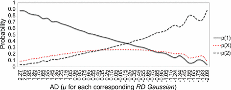
Sensitivity analysis of the 1X2 states of node P, given AD
-
2.
RD: Represents a mixture of 42 ~ Gaussian distributions (one for each state of AD). At its prior state, RD represents the average discrepancy between home and away ratings, and assumes that the difference follows a ~ Gaussian distribution since the actual data-driven histogram of ancestor AD resembles a perfect ~ Gaussian distribution (see AD and RD in Fig. 6). This node takes the resulting provisional team ratings as input in the form of \( {\text{pr}}_{\text{xH}} - {\text{pr}}_{\text{yA}} \).
-
3.
GH/GA: Represent discrete distributions which capture the data-driven histogram of goals scored for each team at home and away grounds, given AD. Note that while these distributions are not meant to be used as predictors for the number of goals scored by each team, they can be used to predict the score difference (in addition to the outcome of interest 1X2).
-
4.
P: Represents a discrete probability distribution for the prediction of interest, with probabilities assigned to each of the three states of the 1X2 distribution.

The parameter learning of the BN model is restricted to match instances where both the home and away teams have already played a minimum of 50Footnote 4 match instances for each specific league and division they participate in. This restriction ensures that team ratings have converged well prior to being considered as training samples by the model. As a result, the size of the training dataset is reduced from 216,743 to 149,772 samples. Tables 9, 10, 11, 12 and 13, in “Appendix A”, present the Conditional Probability Tables (CPTs) for each of the BN model nodes, which are learnt using Maximum Likelihood Estimation for parameter learning, based on the data provided for the competition. Figure 6, in “Appendix B”, illustrates the prior outputs of the BN model.
Furthermore, Fig. 4 illustrates the sensitivity of states 1X2 of node P given AD, and shows that the parameters of the BN model have generalised well over all leagues, divisions and seasons. This is because the probability for a home win over all leagues and divisions across the world maximises at AD = 1, where the home team is assumed to have the greatest advantage over the away team in terms of rating, and decreases linearly with minimum probability observed at AD = 42, when the home team is assumed to be the outsider (and vice versa for the probability for an away win). Additionally, the probability for a draw peaks at AD points 22–24, when neither of the teams is assumed to have the advantage, since the probabilities for the home and away wins are almost equivalent. However, some instability is observed, particularly at the higher ranks of ability difference, and especially when the away team is the strong favourite. This instability may be due to the relatively low sample size associated with some of the higher ranks of AD (refer to Table 3).
4 Worked example of Dolores
4.1 Predicting match outcomes from team ratings
The worked example is based on the Leicester City versus Stoke City match, dated April 1st 2017. This match represents one of the 206 future match predictions submitted to the competition. First, we require the prior ratings associated with each of the teams; x for Leicester and y for Stoke. These are:
-
Home prior background rating for team x\( {\text{br}}_{{{\text{xH}}_{t - 1}}} = 0.463014 \).
-
Away prior background rating for team x\( {\text{br}}_{{{\text{xA}}_{t - 1}}} = 0.208624 \).
-
Away prior background rating for team y: \( {\text{br}}_{{{\text{yA}}_{t - 1}}} = 0.037819 \).
-
Home prior background rating for team y: \( {\text{br}}_{{{\text{yH}}_{t - 1}}} = 0.537708 \).
For prediction, we only require the home and away rating priors for home and away teams respectively. First, the algorithm checks if the ϕ criterion is met to determine whether any under/over-performances occur and, in such an event, considers the provisional, rather than the background, ratings. According to Sect. 3.1.2, the optimal values for the parameters required to compute the provisional ratings are δ = 2.5, μ = 0.01, and ϕ = 1. Since ϕ = 1, an under/over-performance can be established only when ϕ <− 1 or ϕ > 1 respectively. Data shows that \( \phi_{\text{cx}} = 3 \) for team x and \( \phi_{\text{cy}} = - 1 \) for team y. Team y does not satisfy the ϕ criterion and hence, their away rating remains unchanged and equal to their away background rating:
Team x does satisfy ϕ > 1 and hence, the algorithm considers the provisional rating:
up from the background rating of 0.463014. These can now be used as input to the BN model in the form of \( {\text{pr}}_{\text{xH}} - {\text{pr}}_{\text{yA}} = 0.466550 - 0.037819 = 0.428730 \). The BN model can be constructed as discussed in Sect. 3.2, and with reference to the CPTs provided in “Appendix A”. Furthermore, Fig. 7 in “Appendix B” illustrates the outputs of all the BN latent nodes associated with the above input. The prediction (i.e., output on node P in Fig. 7) is:
For comparison, the average bookmakers’ odds (Football-Data 2017) associated with this match instance are:
which, following normalisation, convert to
4.2 Revising team ratings from match results
The match outcome was 2-0 in favour of team x (i.e., Leicester City). The next step is to revise both the home and away ratings for both the home and away teams. We first compute the goal difference expectation for x and y respectively:
From this, we can compute the expected goal difference for the match:
Since the observed goal difference is 2 in favour of team x, \( {\text{g}}_{\text{o}} = {\text{g}}_{\text{ox}} - {\text{g}}_{\text{oy}} = 2 - 0 = 2 \), the goal difference error between predicted and observed goal difference is:
We then diminish the impact of the goal difference error for both teams x and y respectively:
We can now revise the background ratings. For this, we also require the optimal λ and γ parameters (see Sect. 3.1.2). Specifically,
-
$$ {\text{br}}_{{{\text{xH}}_{t}}} = {\text{br}}_{{{\text{xH}}_{t - 1}}} + \psi_{x} \left( e \right) \times \lambda = 0.463014 + 1.246290 \times 0.054 = 0.530314 $$
-
$$ {\text{br}}_{{{\text{xA}}_{t}}} = {\text{br}}_{{{\text{xA}}_{t - 1}}} + \left( {{\text{br}}_{{{\text{xH}}_{t}}} - {\text{br}}_{{{\text{xH}}_{t - 1}}} } \right) \times \gamma = 0.208624 + \left( {0.530314 - 0.463014} \right) \times 0.79 = 0.261791 $$
-
$$ {\text{br}}_{{{\text{yA}}_{t}}} = {\text{br}}_{{{\text{yA}}_{t - 1}}} + \psi_{y} \left( e \right) \times\lambda = 0.037819 + \left( { - 1.246290} \right) \times 0.054 = - 0.029481 $$
-
$$ {\text{br}}_{{{\text{yH}}_{t}}} = {\text{br}}_{{{\text{yH}}_{t - 1}}} + \left( {{\text{br}}_{{{\text{yA}}_{t}}} - {\text{br}}_{{{\text{yA}}_{t - 1}}} } \right) \times\gamma = 0.537708 + \left( { - 0.029481 - 0.037819} \right) \times 0.79 = 0.484541 $$
Finally, we need to update the parameter ϕ for both x and y teams. This would be the fourth continuous over-performance for team x; i.e., this is because the expectation was 0.397 goals difference in favour of team x, relative to the observation of 2 goals difference in favour of team x. Similarly, this would be the second continuous under-performance for team y. As a result, \( \phi_{\text{cx}} = 4 \) and \( \phi_{\text{cy}} = - 2 \). Now the ratings are ready to be used for future match prediction (i.e., repeat of Sect. 4.1) and later revised based on future match results (i.e., repeat of Sect. 4.2).
5 Evaluation and discussion
The model is evaluated in terms of both predictive accuracy and profitability against published market odds. This section covers these two methods of predictive evaluation in turn.
5.1 Predictive accuracy
As part of the competition, the RPS function (Epstein 1969) is selected to determine the predictive accuracy of the models. The RPS is shown to be more appropriate in assessing probabilistic football match predictions than other more popular metrics, such as the RMS and Brier score (Constantinou and Fenton 2012). This is because the RPS is a scoring function suitable for evaluating probabilistic outcomes of ordinal, rather than nominal, scale. For example, in the case of predicting the winning lottery number, if the winning number is 10 then a prediction of 11 is no better than a prediction of 49; i.e., they are both equally wrong. However, in the case of football match prediction, if the observed outcome is a home win, then a prediction of a draw is less inaccurate than a prediction of an away win, even though neither of those outcomes occurred; i.e., they are not equally wrong.
The RPS represents the difference between cumulative predicted and observed distributions, and is defined as:
where r is the number of distribution outcomes (r = 3 in our case), pj is the predicted outcome at position j such that pj\( \in \left[ {0, 1} \right] \). for \( j = 1, 2, 3 \) and p1 + p2 + p3 = 1, and ej is the observed outcome at position j such that ej\( \in \left[ {0, 1} \right] \) for \( j = 1, 2, 3 \) and e1 + e2 + e3 = 1.
Table 4 presents the results from the international special issue competition Machine Learning for Soccer, as determined by the RPS function. Dolores, stated as ‘Team ACC’ in Table 4, ranked 2nd in the competition with a predictive error 0.94% higher than the top and 116.78% lower than the bottom participants. The results are based on match predictions submitted for 206 future matches, from 26 different leagues, played from March 31 to April 9 in 2017. Crucially, the predictive accuracy achieved on the test dataset demonstrates lower average predictive error when compared to the training dataset error, and this strongly suggests that the model has not overfitted the data.
In addition to the results from the competition, Table 5 illustrates the predictive accuracy achieved by the model for each of the 52 leagues, and based on match instances from seasons 2014/15 to March 19, 2017 (i.e., data used for optimisation). The leagues are ranked by lowest RPS. Overall, the results show that the predictive accuracy in lower divisions (shaded background) tends to be lower than the predictive accuracy in top divisions. This is because the rating discrepancy between teams in lower divisions tends to be lower, on average, than between teams in top divisions; implying that the difference in team ability between favourites and outsiders in lower divisions is not as high as in top divisions. Specifically, and based on the training dataset used for optimisation (refer to Sect. 3.1.2), the average rating difference between teams in lower divisions is 23.7% lower compared to the average rating difference between teams in top divisions. This also explains why bookmakers’ odds associated with lower division matches tend to be more ‘uncertain’ (i.e., rarely indicate a strong favourite) relative to the odds offered for top division matches.
5.2 Profitability
Naturally, the performance of a football model can also be determined by its ability to generate profit against published market odds. In Constantinou et al. (2013) we argued that it can be misleading to focus the evaluation of a football model solely on maximising or minimising a scoring function because (a) different scoring functions can generate different conclusions about which model is ‘best’, and (b) in financial domains researchers demonstrated a weak relationship between the various accuracy metrics and actual profitability (Leitch and Tanner 1991).
On the other hand, profitability-based evaluations exhibit other kind of limitations and hence, it would be best to report results based on both accuracy and profitability metrics. Specifically, profitability depends on:
-
1.
The published market odds, which differ depending on the selected bookmaker for validation purposes. However, in Constantinou and Fenton (2013b) we showed that the divergence in odds between bookmaking firms is limited to the point that arbitrage opportunities are eliminated or, otherwise, minimised.
-
2.
The bookmakers’ incorporated profit margin, which is also known as the ‘over-round’, and represents the ‘unfair’ advantage introduced in published market odds, to practically guarantee profit for the houseFootnote 5 over time. In Constantinou and Fenton (2013b) we showed that while the discrepancy in profit margins between bookmakers decreases over time due to competition, they can still differ considerably between online bookmakers and hence, the selection of the bookmaker can have a significant impact on profitability.
-
3.
The betting strategy, which is an important decision making problem. Betting decision making is normally based on a discrepancy threshold associated with the difference between predicted and bookmakers’ probabilities (converted from odds), in favour of the model in terms of payoff. The value of the bet is either fixed throughout the betting simulation, or determined by the Kelly criterion (Kelly 1956).
-
4.
The interpretation of the results, which is typically based on the return-on-investment (ROI) or the net profits. In Constantinou et al. (2013) we argued that ROI can be a misleading figure. Consider the following two scenarios:
-
a.
Model A suggests two £100 bets and both are successful (100% winning rate), returning a net profit of £200, which represents a ROI of 100%.
-
b.
Model B suggests five £100 bets and four of them are successful (80% winning rate), returning a net profit of £300, which represents a ROI of 60%.
-
a.
A profitability evaluator based on ROI would have erroneously considered model B as being inferior at maximising profit than model A. This is because it fails to consider the possibility that model A might have failed to discover all of the potential betting opportunities in the same way model B did. Conversely, a model which maximises ROI can still be useful in cases where we are interested in minimising the risk of negative returns in exchange for a lower expected net profit.
In this paper, both the ROI and net profit figures are reported. However, betting decision making is optimised for net profits and not for ROI. Specifically, profitability figures:
-
1.
Are based on Football-Data (2017), which captures the published market odds offered by a number of bookmakers over many leagues. The odds are recorded on Friday afternoons for weekend games and on Tuesday afternoons for midweek games.
-
2.
Consider the maximum bookmakers’ odds, which represent the best available odds over a number of fixed odds bookmakers (e.g. excluding Betfair Exchange odds).
-
3.
Are based on all the leagues offered by Football-Data (2017); a total of 21 leagues, where 11 are top divisions and 10 are lower divisions, starting from season 2010/11 to March 2017.
-
4.
Do not assume that the profit margin is eliminated, which hovers between − 0.04 and 1.63%, for the best available odds (as discussed in (2) above).
-
5.
Do not take advantage of any arbitrage opportunities that may arise between bookmakers’ odds.
-
6.
Are based on the typical betting decision strategy whereby a bet is simulated on the outcome of a match instance that offers a payoff which exceeds a predetermined level of discrepancy between predicted and offered odds, in terms of probability. The discrepancy threshold found to maximise overall net profits is 8% (absolute). If more than one outcome meet the discrepancy threshold, only the outcome with the highest discrepancy is chosen for betting.
Tables 6 and 7 provide the results on profitability from betting simulations, for top and lower divisions respectively. In both tables, the results are ranked by lowest profit margin. Overall, the results illustrate marginal profits over all top division leagues and marginal losses over all lower division leagues. The discrepancy in profitability between top and lower divisions could be explained by the higher profit margins incorporated into the odds associated with the lower division matches. However, lower profit margins do not necessarily imply higher profitability (as shown later in this section). Over all of the 21 leagues, and approximately 7 seasons of betting simulations, the model has invested £12,100 in bets (i.e., 12,100 bets of £1 each) and generated £12,069.65 in winnings. Curiously, the model performs relatively well when it comes to the top European football leagues, such as the Spanish La Liga and especially the EPL. Note that the top European leagues, including the German Bundesliga, tend to generate the largest betting volumes and this increases their importance in terms of competition between bookmakers, which partly explains why they incorporate the lowest profit margins.
It has long been assumed that enormous betting volumes dictate a part of the odds; a way for bookmakers to exchange marginal levels of predictive accuracy to maximise profits. Odds which are biased due to betting volumes can be exploited by predictive models. This study supports this assumption based on the high profitability generated on match instances of the EPL, which is by far the most popular football league. It is also crucial to note that the popularity of the EPL has also made it the most likely choice for assessing football match prediction models in the academic literature. This is problematic because, as shown in Tables 6 and 7, the level of profitability observed on match instances of the EPL does not repeat for any of the residual 20 leagues. Additionally, the results show that the profitability between seasons, based on bets ranging from 76 to 135 per EPL season, is not consistent and ranges between − 6.4 and 38% ROI, or − £6.5 and £39.7 net profits.
Table 8 illustrates the overall profitability per football season, over all of the 21 leagues. The results show that while the profit margins have been steadily decreasing over time, and while lower profit margins tend to promise greater returns, this has not resulted into increased profitability. It is important to note that lower profit margins translate into greater payoffs, and which subsequently increase the betting frequency due to a greater number of match instances satisfying the criteria for simulating a bet (assuming the betting decision threshold remains constant). The change in betting frequency does not necessarily translate into increased profitability. This behaviour invites future research on dynamic betting decision thresholds driven by profit margins. It is worth mentioning that the bookmakers who offer betting exchange services (not considered in this study), such as Betfair, enable bettors to minimise profit margins normally below 0.5%, but with a commission fee on winnings up to 5%, which can be discounted depending on betting activity.
Further to what has been discussed in Sect. 5.1, and with reference to Table 5 and Fig. 5 illustrates the ROIFootnote 6 generated for top divisions (left chart) and lower divisions (middle chart), ordered by highest predictive accuracy; i.e., lower RPS. In both cases, the results weakly suggest that the higher the unpredictability of a league, the higher the profitability. However, this outcome contradicts the results presented in Tables 6 and 7, which indicate that profitability decreases for lower divisions that are generally associated with higher unpredictability. Nonetheless, segregating each of the top and lower divisions by season (right graph), for a total of 143 leagues (21 leagues over approximately seven seasons), and ordering them by lower RPS as in previous cases, reveals that unpredictability does indeed weakly associate with higher profits (the linear trend starts and ends at approximately − 2.5 and 4% ROI).

The ROI generated for top divisions (left), lower divisions (middle), and all divisions segregated by season (right) and ordered by higher predictive accuracy (lower RPS). Linear trend is superimposed as a dashed line
6 Concluding remarks
The paper described Dolores, which is a model designed to predict football match outcomes from all over the world, as part of the international special issue competition Machine Learning for Soccer. The model is novel in its approach which is based on (a) dynamic ratings for temporal analysis, and (b) a hybrid BN model that takes the resulting ratings from (a) as input to infer the 1X2 distribution. The model was trained with a dataset of 52 leagues, which includes different divisions from 35 countries. Unlike past relevant literature, this model is designed in a way that enables it to predict football match outcomes of teams in one country by observing match outcomes of teams in multiple countries.
The predictive accuracy of Dolores was assessed as part of the competition, which involved predicting 206 future match instances from different leagues during March in 2017. The paper extends the assessment of the model to a profitability-based validation, based on bookmakers’ odds from 21 different leagues and over a period of approximately seven football seasons. The results indicate marginal profits of 1.09% ROI over all top divisions, and marginal losses of − 1.57% ROI over all lower divisions. While the overall ROIFootnote 7 is not impressive, it still serves as empirical proof that the model, which was solely based on goal data, has generalised well over all leagues and divisions, even accounting for the missing data incorporated into the dataset as part of the challenge. Furthermore, while detailed historical performance for each team is typically required to maximise predictive accuracy, Dolores provides empirical proof that a model can make a good prediction for a match outcome between teams x and y even when the prediction is derived from historical match data that neither x nor y participated in.
Further to profitability, it is important to note that relevant academic literature is often driven by profitability from betting simulations on match instances of the EPL. In many cases, these results are based on a single season of the EPL. Interestingly, Dolores generated 20% + ROI based on approximately seven seasons of the EPL; a rather impressive performance. However, as shown in Tables 6 and 7, this level of profitability is not repeated for any of the residual 20 leagues taken into consideration. Given that the EPL is the most popular league, this enforces the popular hypothesis that the enormous betting volumes dictate part of the published market odds, and this enables predictive models to exploit such inaccuracies. Moreover, the results show that profitability between seasons of the same league is not consistent. In the case of the EPL, and over seven seasons of betting simulations, annual profitability ranges between − 6.4 and 38% ROI. These all-inclusive results raise some concerns about the validity of conclusions in past relevant literature. This is because, while there is nothing wrong with demonstrating that a model can identify such (possibly) biased odds and generate profit from bets on match instances of the EPL, there is still a risk that such results will be misinterpreted as generic and independent of the EPL. The results from this study also suggest that it would be best to extend assessments of profitability over multiple seasons.
Finally, past studies have shown that it is possible to increase the predictive accuracy of a model by incorporating other key factors, such as player transfers, availability of key players, participation in international competitions, new coach, level of injuries, attack and defence ratings, and even team motivation/psychology in the form of expert knowledge (Constantinou et al. 2012; Pena 2014; Szczepanski and McHale 2015; Constantinou and Fenton 2017). Because of the competition requirements and the multiple leagues captured by the dataset, the model presented in this paper had to be restricted to goal scoring data. Future work will investigate ways to extend Dolores towards accounting for such additional key factors of interest.
Notes
The reverse assumption had also been examined and was found to decrease predictive accuracy.
Constantinou and Fenton (2013a) proposed the function ψ(e) to diminish the importance of high score differences. While in both studies the function appears to adequately capture the importance of high score differences, a weakness of this function is that it is deterministic, in exchange for reduced model complexity.
The minimum sample size is 32 at R = 41.
In Constantinou and Fenton (2013a), 30 iterations of rating development were found to be sufficient in the case of the EPL. In this study, the number of iterations has been increased to 50, even though the learning rates are higher and promise faster convergence of the ratings. This is because, in this study, we generalise the model over 52 leagues and hence, it is more than likely that some leagues exist in which the rating difference between the strongest and weakest teams is considerably higher relative to the respective difference when only focusing on the EPL, as in the original study.
This ‘unfairness’ is similar to the payoffs offered on roulette where the house has an edge, or a profit margin, of 1/37 (or 2.7%) in the case of the European roulette, and 2/38 (or 5.26%) in the case of the American version.
ROI has been chosen over the net profits to ensure that the graphs in Fig. 5 do not generate a trend that is biased towards the number of bets simulated per league.
Note that the betting strategy was optimised for net profits rather than ROI [refer to Sect. 5.2, point (iv)].
References
Angelini, G., & Angelis, L. D. (2017). PARX model for football match predictions. Journal of Forecasting, 36, 795.
Arabzad, S. M., Araghi, M. E. T., Sadi-Nezhad, S., & Ghofrani, N. (2014). Football match results prediction using artificial neural networks; The case of Iran Pro League. International Journal of Applied Research on Industrial Engineering, 1(3), 159–179.
Baio, G., & Blangiardo, M. (2010). Bayesian hierarchical model for the prediction of football results. Journal of Applied Statistics, 37(2), 253–264.
Berrar, D., Dubitzky, W., Davis, J., & Lopes, P. (2017). Machine learning for soccer. Retrieved September 1, 2017 from https://osf.io/ftuva/.
Britannica. (2017). Football (Association Football, Soccer). In Encyclopaedia Britannica, Retrieved April 19, 2017 from https://www.britannica.com/sports/football-soccer.
Cheng, T., Cui, D., Fan, Z., Zhou, J., & Lu, S. (2003). A new model to forecast the results of matches based on hybrid neural networks in the soccer rating system. In IEEE Xplore.
Constantinou, A. C., & Fenton, N. E. (2012). Solving the Problem of Inadequate Scoring Rules for Assessing Probabilistic Football Forecast Models. Journal of Quantitative Analysis in Sports, 8(1), 1–14.
Constantinou, A. C., & Fenton, N. E. (2013a). Determining the level of ability of football teams by dynamic ratings based on the relative discrepancies in scores between adversaries. Journal of Quantitative Analysis in Sports, 9(1), 37–50.
Constantinou, A. C., & Fenton, N. E. (2013b). Profiting from arbitrage and odds biases of the European football gambling market. The Journal of Gambling Business and Economics, 7(2), 41–70.
Constantinou, A., & Fenton, N. (2017). Towards smart-data: Improving predictive accuracy in long-term football team performance. Knowledge-Based Systems, 124, 93–104.
Constantinou, A. C., Fenton, N. E., & Neil, M. (2012). pi-football: A Bayesian network model for forecasting Association Football match outcomes. Knowledge-Based Systems, 36, 322–339.
Constantinou, A. C., Fenton, N. E., & Neil, M. (2013). Profiting from an inefficient Association Football gambling market: Prediction, Risk and Uncertainty using Bayesian networks. Knowledge-Based Systems, 50, 60–86.
Daily Mail. (2015). Global sports gambling worth ‘up to $3 trillion’. Daily Mail. Retrieved April 19, 2017 from http://www.dailymail.co.uk/wires/afp/article-3040540/Global-sports-gambling-worth-3-trillion.html.
Dayaratna, K. D., & Miller, S. J. (2013). The Pythagorean won-loss formula and hockey: A statistical justification for using the classic baseball formula as an evaluative tool in hockey (pp. 193–209). XVI: The Hockey Research Journal.
Deloitte. (2016). Annual Review of Football Finance 2016. Deloitte. Retrieved April 19, 2017 from https://www2.deloitte.com/uk/en/pages/sports-business-group/articles/annual-review-of-football-finance.html.
Dixon, M. J., & Coles, S. G. (1997). Modelling association football scores and inefficiencies in the football betting market. Applied Statistics, 46(2), 265–280.
Dunning, E. (1999). The development of soccer as a world game. In Sports Matters: Sociological Studies of Sport Violence and Civilisation. London: Routledge.
Elo, A. E. (1978). The rating of chess players, past and present. New York: Arco Publishing.
Epstein, E. (1969). A scoring system for probability forecasts of ranked categories. Journal of Applied Meteorology, 8, 985–987.
FIFA. (2017). FIFA/Coca-Cola World Ranking. FIFA. Retrieved April 19, 2017 from http://www.fifa.com/fifa-world-ranking/procedure/men.html.
Football-Data. (2017). Historical Football Results and Betting Odds Data. Retrieved April 4, 2017 from http://www.football-data.co.uk/data.php.
Forrest, D., Goddard, J., & Simmons, R. (2005). Odds-setters as forecasters: The case of English football. International Journal of Forecasting, 21, 551–564.
Gelman, A., Carlin, J., Stern, H., & Rubin, D. (2003). Bayesian data analysis (2nd ed.). Boca Raton: Chapman and Hall/CRC.
Goddard, J. (2005). Regression models for forecasting goals and match results in association football. International Journal of Forecasting, 21, 331–340.
Goddard, J., & Asimakopoulos, I. (2004). Forecasting football results and the efficiency of fixed-odds betting. Journal of Forecasting, 23, 51–66.
Hamilton, H. (2011). An extension of the pythagorean expectation for association football. Journal of Quantitative Analysis in Sports, 7(2), 1–18.
Huang, K., & Chang, W. (2010). A neural network method for prediction of 2006 World Cup Football Game. In IEEE Xplore.
Hvattum, L. M., & Arntzen, H. (2010). Using ELO ratings for match result prediction in association football. International Journal of Forecasting, 26, 460–470.
Joseph, A., Fenton, N., & Neil, M. (2006). Predicting football results using Bayesian nets and other machine learning techniques. Knowledge-Based Systems, 7, 544–553.
Karlis, D., & Ntzoufras, I. (2003). Analysis of sports data by using bivariate Poisson models. Journal of the Royal Statistical Society: Series D (The Statistician), 52(3), 381–393.
Kelly, J. L. (1956). A new interpretation of information rate. Bell System Technical Journal, 35(4), 917–926.
Koller, D., & Friedman, N. (2009). Probabilistic graphical models: Principles and techniques. Cambridge: The MIT Press.
Kuypers, T. (2000). Information and efficiency: An empirical study of a fixed odds betting market. Applied Economics, 32, 1353–1363.
Lee, A. J. (1997). Modeling scores in the Premier League: Is Manchester United really the best? Chance, 10(1), 15–19.
Leitch, G., & Tanner, J. E. (1991). Economic forecast evaluation: Profits versus the conventional error measures. American Economic Association, 81(3), 580–590.
Leitner, C., Zeileis, A., & Hornik, K. (2010). Forecasting sports tournaments by ratings of (prob)abilities: A comparison for the EURO 2008. International Journal of Forecasting, 26, 471–481.
Maher, M. J. (1982). Modelling association football scores. Statistica Neerlandica, 36(3), 109–111.
Miller, S. J. (2006). A derivation of the pythagorean won-loss formula in baseball. arXiv:math/0509698 [math.ST].
O’Shaughnessy, D. (2006). Possession versus position: Strategic evaluation in AFL. Journal of Sports Science & Medicine, 5(4), 533–540.
Oliver, D. (2004). Basketball on paper: Rules and tools for performance analysis. Washington, DC: Brassey’s Inc.
Pearl, J. (1982). Reverend Bayes on inference engines: A distributed hierarchical approach. In AAAI - 82 Proceedings (pp. 133–136).
Pearl, J. (1985). A model of activated memory for evidential reasoning. In Proceedings of the cognitive science society (pp. 329–334).
Pearl, J. (2009). Causality: Models, reasoning and inference (2nd ed.). Cambridge: Cambridge University Press.
Pena, J. L. (2014). A Markovian model for association football possession and its outcomes. arXiv:1403.7993 [math.PR].
Piette, J., Pham, L., & Anand, S. (2011). Evaluating basketball player performance via statistical network modeling. In MIT Sloan Sports Analytics Conference 2011, Boston, MA, USA.
Pomeroy, K. (2017). 2018 Pomeroy College Basketball Ratings. Retrieved November 30, 2017 from https://kenpom.com/.
Rotshtein, A., Posner, M., & Rakytyanska, A. (2005). Football predictions based on a fuzzy model with genetic and neural tuning. Cybernetics and Systems Analysis, 41(4), 619–630.
Rue, H., & Salvesen, O. (2010). Prediction and retrospective analysis of soccer matches in a league. Journal of the Royal Statistical Society: Series D (The Statistician), 49(3), 399–418.
Schatz, A. (2006). Pro football prospectus 2006: Statistics, analysis, and insight for the information age. New York: Workman Publishing Company.
Szczepanski, L., & McHale, I. (2015). Beyond completion rate: Evaluating the passing ability of footballers. Journal of the Royal Statistical Society: Series A (Statistics in Society), 179(2), 513–533.
Tsakonas, A., Dounias, G., Shtovba, S. & Vivdyuk, V. (2002). Soft computing-based result prediction of football games. In The first international conference on inductive modelling (ICIM2002), Lviv, Ukraine.
Acknowledgements
This study was partly supported by the European Research Council (ERC), Research Project ERC-2013-AdG339182-BAYES_KNOWLEDGE.
Author information
Authors and Affiliations
Corresponding author
Additional information
Editors: Philippe Lopes, Werner Dubitzky, Daniel Berrar, and Jesse Davis.
Appendices
Appendix A: Parameterised CPTs of the Hybrid Bayesian Network
Appendix B: Prior and posterior outputs of the Bayesian Network

The prior outputs of the parameterised Bayesian Network model (graph produced in AgenaRisk)

The posterior outputs of the Bayesian Network model based on the worked example of Sect. 4
Rights and permissions
About this article

Cite this article
Constantinou, A.C. Dolores: a model that predicts football match outcomes from all over the world. Mach Learn 108, 49–75 (2019). https://doi.org/10.1007/s10994-018-5703-7
Received:
Accepted:
Published:
Issue Date:
DOI: https://doi.org/10.1007/s10994-018-5703-7