
Abstract
Team semantics is a highly general framework for logics which describe dependencies and independencies among variables. Typically, the (in)dependencies considered in this context are properties of sets of configurations or data records. We show how team semantics can be further generalized to support languages for the discussion of interventionist counterfactuals and causal dependencies, such as those that arise in manipulationist theories of causation (Pearl, Hitchcock, Woodward, among others). We show that the “causal teams” we introduce in the present paper can be used for modelling some classical counterfactual scenarios which are not captured by the usual causal models. We then analyse the basic properties of our counterfactual languages and discuss extensively the differences with respect to the Lewisian tradition.
Article PDF
Notes
We thank Kaibo Xie (personal communication) for this argument.
References
Barbero, F., & Sandu, G. (2017). Team semantics for interventionist counterfactuals and causal dependence. arXiv:1610.03406.
Barbero, F., & Sandu, G. (2019). Interventionist counterfactuals on causal teams. In Finkbeiner, B., & Kleinberg, S. (Eds.) Proceedings 3rd Workshop on Formal Reasoning about Causation, Responsibility, and Explanations in Science and Technology, Thessaloniki, Greece, 21st April 2018. vol. 286 of Electronic Proceedings in Theoretical Computer Science, Open Publishing Association (pp. 16–30).
Briggs, R. (2012). Interventionist counterfactuals. Philosophical Studies: An International Journal for Philosophy in the Analytic Tradition 160, 1, 139–166.
Caicedo, X., Dechesne, F., & Janssen, T.M.V. (2009). Equivalence and quantifier rules for logic with imperfect information. Logic Journal of the IGPL, 17, 91–129.
Cameron, P., & Hodges, W. (2001). Some combinatorics of imperfect information. Journal of Symbolic Logic, 66, 673–684.
Ciardelli, I. (2016). Lifting conditionals to inquisitive semantics. Semantics and Linguistic Theory, 26(10), 732.
Ciardelli, I., & Roelofsen, F. (2011). Inquisitive logic. Journal of Philosophical Logic, 40(1), 55–94.
Ciardelli, I., Zhang, L., & Champollion, L. (2018). Two switches in the theory of counterfactuals. Linguistics and Philosophy, 41(6), 577–621.
Corander, J., Hyttinen, A., Kontinen, J., Pensar, J., & Väänänen, J. (2016). A logical approach to context-specific independence. In Logic, Language, Information, and Computation - 23rd International Workshop, WoLLIC 2016, Puebla, Mexico, August 16-19th, 2016. Proceedings (pp. 165–182).
Durand, A., Hannula, M., Kontinen, J., Meier, A., & Virtema, J. (2016). Approximation and dependence via multiteam semantics. In Proceedings of the 9th International Symposium on Foundations of Information and Knowledge Systems, (Vol. LNCS 9616 pp. 271–291): Springer.
Galles, D., & Pearl, J. (1998). An axiomatic characterization of causal counterfactuals. Foundations of Science, 3(1), 151–182.
Galliani, P. (2012). Inclusion and exclusion dependencies in team semantics - on some logics of imperfect information. Annals of Pure and Applied Logic, 163(1), 68–84.
Galliani, P. (2013). Upwards closed dependencies in team semantics. In Proceedings Fourth International Symposium on Games, Automata, Logics and Formal Verification, GandALF 2013, Borca di Cadore, Dolomites, Italy, 29-31th August 2013 (pp. 93–106).
Grädel, E., & Väänänen, J. (2013). Dependence and independence. Studia Logica, 101, 399–410.
Halpern, J. (2016). Actual Causality. MIT Press.
Halpern, J.Y. (2000). Axiomatizing causal reasoning. J. Artif. Int. Res., 12(1), 317–337.
Halpern, J.Y., & Pearl, J. (2005). Causes and explanations: a structural-model approach. part i: Causes. The British Journal for the Philosophy of Science, 56(4), 843–887.
Hausman, D.M. (1998). Causal asymmetries. Cambridge University Press.
Hintikka, J., & Sandu, G. (1989). Informational independence as a semantical phenomenon. In Fenstad, J.E., & et al. (Eds.) Logic, Methodology and Philosophy of Science VIII (pp. 571–589): Elsevier Science Publishers B.V.
Hitchcock, C. (2001). The intransitivity of causation revealed in equations and graphs. The Journal of Philosophy, 98(06), 273–299.
Hitchcock, C. (2001). A tale of two effects. Philosophical Review, 110(3), 361–396.
Hitchcock, C. Causal modelling. In Beebee, H., Hitchcock, C., & Menzies, P. (Eds.) The Oxford Handbook of Causation (p. 2009): Oxford University Press.
Hodges, W. (1997). Compositional semantics for a language of imperfect information. Logic Journal of the IGPL, 5, 539–563.
Hodges, W. (1997). Some strange quantifiers. In Mycielski, J., Rozenberg, G., & Salomaa, A. (Eds.) Structures in Logic and Computer Science. Lecture Notes in Computer sci, (Vol. 1261 pp. 51–65). London: Springer.
Hyttinen, T., Paolini, G., & Väänänen, J. (2015). Quantum team logic and Bell’s inequalities. Review of Symbolic Logic, 08(04), 722–742.
Kaufmann, S. (2013). Causal premise semantics. Cognitive Science, 37(6), 1136–1170.
Kontinen, J., & Nurmi, V. (2009). Team logic and second-order logic. In Ono, H., Kanazawa, M., & de Queiroz, R. (Eds.) Logic, Language, Information and Computation: Lecture Notes in Computer Science 5514 (pp. 230–241). Berlin: Springer.
Lewis, D. (1973). Causation. Journal of Philosophy, 70(17), 556–567.
Lewis, D. (1973). Counterfactuals. Oxford: Blackwell publishers.
Mann, A.L., Sandu, G., & Sevenster, M. (2011). Independence-Friendly logic - a game-theoretic approach, vol. 386 of London Mathematical Society lecture note series. Cambridge University Press.
McGee, V. (1985). A counterexample to modus ponens. Journal of Philosophy, 82(9), 462–471.
Pearl, J. (2000). Causality: Models, Reasoning, and Inference. New York: Cambridge University Press.
Pearl, J., Glymour, M., & Jewell, N.P. (2016). Causal inference in statistics: a primer. John Wiley & Sons.
Sano, K., & Virtema, J. (2015). Axiomatizing propositional dependence logics. In Kreutzer, S. (Ed.) 24th EACSL Annual Conference on Computer Science Logic. Leibniz International Proceedings in Informatics (LIPIcs), Schloss Dagstuhl–Leibniz-Zentrum fuer Informatik, pp. 292–307. Volume: 41 Proceeding volume.
Schulz, KK. (2011). “If you’d wiggled A, then B would’ve changed”. Causality and counterfactual conditionals Synthese 179 (03).
Schulz, K. (2018). The similarity approach strikes back: negation in counterfactuals. In Sauerland, U, & Solt, S (Eds.) Proceedings of Sinn und Bedeutung 22 (pp. 343–360).
Sider, T. (2010). Logic for Philosophy Vol. 304. Oxford: Oxford University Press.
Spirtes, P., Glymour, C., & Scheines, R.N. (1993). Causation Prediction, and Search, vol. 81 of Lecture Notes in Statistics. New York: Springer.
Stalnaker, R.C. (1968). A theory of conditionals. Americal Philosophical Quarterly, pp 98–112.
Väänänen, J. (2007). Dependence logic: a new approach to Independence Friendly logic, vol. 70 of London Mathematical Society Student Texts. Cambridge University Press.
Väänänen, J. (2008). Modal dependence logic, new perspectives on games and interaction. In Apt, K., & van Rooij, R. (Eds.) Vol. 5 of texts in logic and games (pp. 237–254): Amsterdam University Press.
Veltman, F. (2005). Making counterfactual assumptions. Journal of Semantics 22, 2(05), 159–180.
von Wright, G.H. (1971). Explanation and Understanding. Ithaca: Cornell University Press.
Woodward, J. (2001). Probabilistic causality, direct causes and counterfactual dependence. Stochastic Causality, pp 39–63.
Woodward, J. (2003). Making things happen, vol. 114 of Oxford Studies in the Philosophy of Science. Oxford University Press.
Yang, F. (2017). Uniform definability in propositional dependence logic. The Review of Symbolic Logic, 10(1), 65–79.
Yang, F., & Väänänen, J. (2016). Propositional logics of dependence. Annals of Pure and Applied Logic, 167(7), 557–589.
Yang, F., & Väänänen, J. (2017). Propositional team logics. Annals of Pure and Applied Logic, 168(7), 1406–1441.
Zhang, J. (2013). A Lewisian logic of causal counterfactuals. Minds and Machines, 23(1), 77–93.
Acknowledgements
Open access funding provided by University of Helsinki including Helsinki University Central Hospital. The research was conducted under the aid of the Academy of Finland grants n. 286991 and n. 316460. The authors wish to thank Ivano Ciardelli for carefully reading and commenting upon an earlier version of the paper; and the anonymous reviewers and the editor for many significant suggestions.
Author information
Authors and Affiliations
Corresponding author
Additional information
Publisher’s Note
Springer Nature remains neutral with regard to jurisdictional claims in published maps and institutional affiliations.
Appendices
Appendix A: Distance Between Variables in a Graph
We specify here the notion of distance that we have used in the definition of the do algorithm. Suppose we are given a graph G = (V, E); in the context of this paper, the vertices V are thought of as variables. The general intuition is that, after an intervention on X, other variables should be updated; and variables at distance n + 1 can only be updated after the variables at distance ≤ n have been updated.
We define the distance between two variables X and Y to be the maximum length of a directed path from X to Y:
if any such paths exists; or − 1 otherwise.
Clearly, if the graph is finite and acyclic, \(d_{G}(X,Y)\in \mathbb {N}\cup \{-1\}\) for any pair X, Y. We omit the subscript G when the graph is clear from the context. Notice that in an acyclic graph dG(X, Y ) ≠ dG(Y, X) whenever X and Y are distinct variables.
The algorithm described in Section 2 uses this notion of distance in order to define interventions of the form do(X = x). However, as we saw, we needed to define the more general notion of intervention of the form do(X = x). This can be achieved by defining a notion of distance between a set of variables X and a variable Y; we denote it by dG(X,Y). There are two ideas involved in this generalization. The first is that we should not count the directed paths that are disrupted by the intervention itself (an intervention do(X = x) removes all arrows coming into variables of X); for this purpose, we need to consider the reduced graph G−X = (V, E−X), the graph obtained by removing all arrows going into some vertex of X (i.e., an edge (V1,V2) is in E−X iff it is in E and V2∉X). The second idea is that we should take the maximum of the individual distances between each variable X of X and Y (relative to the reduced graph). Thus we obtain
Let X = x be a consistent conjunction (i.e. it does not contain pairs of formulas \(X=x, X=x^{\prime }\) with \(x \neq x^{\prime }\)). An algorithm for do(X = x) is then obtained by modifying the algorithm for do(X = x) as follows:
-
Stage 0 is replaced with: produce the team T0 by replacing each assignment s ∈ T− with s(x/X).
-
Replace dG(X, Y ) with dG(X, Y ).
We do not define the algorithm for inconsistent conjunctions.
Using Theorem 4.1, it can be proved (see [1]) that the intervention do(X = x) (for consistent X = x) could be equivalently defined as the sequential application of individual interventions do(X = x), for each conjunct X = x in X = x, applied in any order.
Appendix B: Proof of the Termination of the do Algorithm
Theorem B.1
Let T be a recursive causal team. If GT is a finite acyclic graph, then TX=x is well-defined.
Proof
Assume, at first, that T− is finite.
Suppose that, for \(\mathbf {X}\subseteq Dom_{T}, Y\in Dom_{T}\), d(X, Y ) > card(GT). Then there is a path P in \(G_{T}^{-\mathbf { X}}\) from some X ∈X to Y such that length(P) > card(GT). Then there is a node which is crossed at least twice by P; so \(G_{T}^{-\mathbf { X}}\) contains a cycle. Therefore, the larger graph GT contains a cycle, and we have a contradiction. Thus, sup{d(X, Z) | Z ∈ DomT}≤ card(GT); this means that the “for” cycle in the algorithm goes through a finite number of iterations over the variable n.
Finally, notice that, for each n, the number of variables Z such that d(X, Z) = n is finite (due to finiteness of GT), as is the number of assignments t in the team that is undergoing modification (due to the finiteness of T−). Therefore, the algorithm terminates after a finite number of steps.
If instead T− is infinite, (TX=x)− is produced by an infinitary algorithm which, in each iteration of the “for” cycle, performs simultaneously the substitution \(t \hookrightarrow t(f_{Z_{1}}(s(PA_{Z_{1}}))/Z_{1}, \dots , f_{Z_{k_{n+1}}}(s(PA_{Z_{k_{n+1}}}))/Z_{k_{n+1}})\) for all the assignments t in the current team. By the arguments above, such an “algorithm” terminates and yields a well-defined causal team. □
Appendix C: Complete Axiomatization for Language \(\mathcal {CO}\)
As pointed out in the main text, for any given signature σ = (Dom, Ran), a complete inference system for the language \(\mathcal {CO}(\sigma )\) (interpreted over causal teams of signature σ) can be obtained by adapting and slightly extending the axiomatization proposed by Halpern [16] for a language interpreted over causal models. See Section 4.1 for the list of axioms and rules.
Under many respects, our framework is closer to that of Briggs [3], in that 1) our notion of signature does not encode a distinction between exogenous and endogenous variables, 2) our language treats exogenous and endogenous variables on a par, e.g. by allowing interventions over both. Because of these differences from Halpern’s approach, our strategy for obtaining the completeness proof will be closer to that used in [3].
The notion of consequence that we want to axiomatize is Γ⊧σψ: every recursive causal team of signature σ which satisfies all formulas in Γ also satisfies ψ. We write Γ ⊩σψ to say that ψ is the end formula of some proof in \(Ax_{\mathcal {C}\mathcal {O}}(\sigma )\) which possibly uses extra premises from Γ.
The soundness of the axioms can be proved by observing their soundness over causal teams with singleton team components; and then using the flatness of \(\mathcal {CO}(\sigma )\) (Theorem 2.10). The soundness of many of the rules has been addressed in the main text; the following lemmas yield a general method for proving the soundness of the inference rules of \(AX_{\mathcal {C}\mathcal {O}}(\sigma )\).
Lemma C.1
The inference rules of \(AX_{\mathcal {CO}}(\sigma )\) are sound for recursive causal teams with singleton team component.
Given the obvious identification of deterministic structural equation models with causal teams with singleton team component, this soundness result follows from the literature [3, 11, 16]. Next we show how to extend this result to all recursive causal teams.
Lemma C.2
Let \({\Gamma }\cup \{\psi \}\subseteq \mathcal {CO}(\sigma )\), and suppose that every causal team which has singleton team component and satisfies Γ also satisfies ψ. Then Γ⊧σψ.
Proof
Let T be a recursive causal team, and suppose that T⊧Γ and T⊮ψ. From the latter, plus flatness of ψ (Theorem 2.10), it follows that there is an s ∈ T− such that (*) {s}⊮ψ. By T⊧Γ and the flatness of Γ, it follows that (**) {s}⊧Γ. (*) and (**), together, contradict the assumption that Γ entails ψ over recursive causal teams with singleton component. □
We point out that the following principles are also sound for recursive causal teams (as can be proved by the two previous lemmas):
-
Composition 2:
 .
. -
Reversibility:
 (for Y ≠ W).
 .
. (for Y ≠ W).
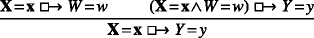
Composition 2 is a “converse” to Composition 1. It was implicitly part of the axiom system of Galles and Pearl [11], but [16] showed that it is unnecessary for a completeness proof.
What we now show is that (for each signature σ) the system \(AX_{\mathcal {CO}}(\sigma )\) is complete for ⊧σ. The strategy will be to show that every consistent set of formulas has a model; we mostly follow the method used in [3]. There is some vagueness in the literature as to what notion of (proof-theoretic) consistency is involved here; the notion we will use is given in the definition below. But first a notational convention. Given a set Γ of \(\mathcal {C}\mathcal {O}(\sigma )\) formulas, write \({\Gamma }^{\vdash }_{\sigma }\) for its closure under deduction in \(AX_{\mathcal {C}\mathcal {O}}(\sigma )\).
Definition C.3
A set Γ of \(\mathcal {CO}(\sigma )\) formulas is σ-consistent if \({\Gamma }^{\vdash }_{\sigma }\) does not contain any pair of formulas of the form ψ, ¬ψ.
Γ is maximally σ-consistent if it is σ-consistent and every \({\Gamma }^{\prime }\supset {\Gamma }\) is not σ-consistent.
In the following we shall simply write “consistent” for σ-consistent, since the relevant signature will be clear from the context.
We note that, since \(AX_{\mathcal {CO}}(\sigma )\) contains all instances of classical tautologies and modus ponens, one can prove the syntactical deduction theorem as usual.
Lemma C.4
Let ψ, χ be \(\mathcal {CO}(\sigma )\) formulas. Then
Lemma C.5
Let Γ be a consistent set of \(\mathcal {CO}(\sigma )\) formulas, and ψ a \(\mathcal {CO}(\sigma )\) formula. Suppose Γ⊯σψ; then Γ ∪{¬ψ} is consistent.
Proof
Suppose Γ ∪{¬ψ} is not consistent; then Γ ∪{¬ψ}⊩σχ and Γ ∪{¬ψ}⊩σ¬χ for some \(\mathcal {CO}(\sigma )\) formula χ. Then, using Lemma C.4, we get that \({\Gamma } \vdash _{\sigma } \neg \psi \supset \chi \) and \({\Gamma } \vdash _{\sigma } \neg \psi \supset \neg \chi \). Using classical logic we get Γ ⊩σψ, contradicting the assumption. □
Using this result, one can prove as usual a version of Lindenbaum’s lemma.
Lemma C.6
Let Γ be a consistent set of \(\mathcal {CO}(\sigma )\) formulas. Then there is a maximally consistent set Δ of \(\mathcal {CO}(\sigma )\) formulas such that \({\Gamma }\subseteq {\Delta }\).
Lemma C.5 also entails that maximally consistent sets of formulas are syntactically complete:
Corollary C.7
Let Δ be a maximally consistent set of \(\mathcal {CO}(\sigma )\) formulas. Then, for every \(\psi \in \mathcal {CO}(\sigma )\), either ψ ∈Δ or ¬ψ ∈Δ.
In the next lemma we prove that a maximally consistent set of \(\mathcal {CO}(\sigma )\) formulas “uniquely determines” the outcome of interventions.
Lemma C.8
Let σ = (Dom, Ran) be a signature, \(\mathbf { X}\cup \{Y\}\subseteq Dom\), X ≠ ∅. Let Δ be a maximally consistent set of \(\mathcal {CO}(\sigma )\) formulas.
-
1.
There is exactly one y ∈ Ran(Y ) such that “Y = y” ∈Δ.
-
2.
For every x ∈ Ran(X) there is exactly one y ∈ Ran(Y ) such that
 .
.
 .
.Proof
Let us prove 2. Let x ∈ Ran(X). First we show that Δ can contain a formula of the form  for at most one value y ∈ Ran(Y ). Indeed, let \(y^{\prime }\) be a distinct value in Ran(Y ); observe that Δ is closed under ⊩σ, and thereby under applications of the Uniqueness rule; so, since
  , we obtain that
  . But notice that this formula is
  (by definition of the dualization). So, by the consistency of Δ,
  .
.
We then have to show that there is at least one y ∈ Ran(Y ) such that  . For suppose this is not the case; then by maximality of Δ, corollary C.7 and the definition of dual negation,
  for each y ∈ Ran(Y ); thus
  . But this formula is just
  ; and
; and  by the Definiteness axiom. Since Δ is consistent, we have reached a contradiction.
The proof of 1. is analogous, using instances of Uniqueness and Definiteness with empty antecedents. □
We will need two substitution lemmas to guarantee that rules need not be applied to the outermost connectives of a formula. The first is for formulas that occur in positive contexts. We write φ[𝜃] for a formula if we want to highlight that it has an (occurrence of) a subformula 𝜃. If \(\theta ^{\prime }\) is yet another formula, \(\varphi [\theta ^{\prime }]\) will denote the formula which results by substituting the occurrence 𝜃 with \(\theta ^{\prime }\) in φ.
Lemma C.9
Let \(\varphi [\theta ],\theta ^{\prime }\in \mathcal {CO}(\sigma )\) and let 𝜃 denote a specific occurrence of a subformula of φ[𝜃]. Assume further that 𝜃 is not occurring in any antecedent of \(\supset \) or  . If \(\theta \vdash _{\sigma } \theta ^{\prime }\), then \(\varphi [\theta ]\vdash _{\sigma } \varphi [\theta ^{\prime }]\).
Proof
We prove it by induction on φ[𝜃], including more generally the possibility that 𝜃 does not occur at all in φ[𝜃]. First base case: φ[𝜃] is 𝜃. Then \(\theta \vdash _{\sigma } \theta ^{\prime }\) by assumption, and \(\theta ^{\prime }\) is \(\varphi [\theta ^{\prime }]\). Second base case: φ[𝜃] does not contain the intended occurrence of 𝜃. Then \(\varphi [\theta ^{\prime }] = \varphi [\theta ]\), from which obviously \(\varphi [\theta ] \vdash _{\sigma } \varphi [\theta ^{\prime }]\).
Inductive step: φ[𝜃] is ψ[𝜃] ∘ χ[𝜃], where ∘ is one of the binary connectives of \(\mathcal {CO}(\sigma )\). By the inductive hypothesis, \(\psi [\theta ]\vdash _{\sigma } \psi [\theta ^{\prime }]\) and \(\chi [\theta ]\vdash _{\sigma } \chi [\theta ^{\prime }]\). The cases for ∧ and ∨ follow easily using classical tautologies; we prove the remaining cases.
-
∘ is \(\supset \). Since the occurrence 𝜃 is not in ψ[𝜃], we have \(\psi [\theta ]=\psi [\theta ^{\prime }]\); but then \(\neg \psi [\theta ]\vdash _{\sigma } \neg \psi [\theta ^{\prime }]\). Furthermore, by the inductive hypothesis, \(\chi [\theta ]\vdash _{\sigma } \chi [\theta ^{\prime }]\). By lemma C.4 we get \(\vdash _{\sigma } \neg \psi [\theta ^{\prime }]\supset \neg \psi [\theta ]\) and \(\vdash _{\sigma } \chi [\theta ]\supset \chi [\theta ^{\prime }]\).
Since \(\vdash _{\sigma } (\neg \psi [\theta ^{\prime }]\supset \neg \psi [\theta ]) \supset ((\chi [\theta ]\supset \chi [\theta ^{\prime }]) \supset ((\psi [\theta ]\supset \chi [\theta ])\supset (\psi [\theta ^{\prime }]\supset \chi [\theta ^{\prime }]))\), as this is an instance of a classical tautology, by two applications of Modus ponens we get \(\vdash _{\sigma }(\psi [\theta ]\supset \chi [\theta ])\supset (\psi [\theta ^{\prime }]\supset \chi [\theta ^{\prime }])\). By lemma C.4, then, \(\psi [\theta ]\supset \chi [\theta ]\vdash _{\sigma } \psi [\theta ^{\prime }]\supset \chi [\theta ^{\prime }]\).
-
∘ is
 . Since by inductive hypothesis we have \(\chi [\theta ]\vdash _{\sigma } \chi [\theta ^{\prime }]\), and furthermore \(\psi [\theta ]=\psi [\theta ^{\prime }]\), by applying the C-substitution rule we obtain:

 . Since by inductive hypothesis we have
□
The second substitution lemma guarantees substitution of equivalents in the antecedents of counterfactuals occurring in the context of a complex formula.
Lemma C.10
Let ψ[X = x] be a \(\mathcal {CO}(\sigma )\) formula without occurrences of \(\supset \). Suppose the occurrence of X = x is in the antecedent of a counterfactual occurring in ψ[X = x]. If X = x ⊣⊩σZ = z, then ψ[X = x] ⊣⊩σψ[Z = z].
Proof
The proof is analogous to that of lemma C.9, using A-substitution instead of C-substitution. □
The next lemma shows how to build an appropriate “model” for any maximally consistent set of \(\mathcal {CO}(\sigma )\) formulas.
Lemma C.11
Let σ = (Dom, Ran) be a signature, and Δ be a maximally consistent set of \(\mathcal {CO}(\sigma )\) formulas. Then there is a recursive causal team T of signature σ such that T− is a singleton, and T⊧Δ.
Proof
-
1)
Defining T. Suppose first that card(Dom) ≥ 2. For each variable V ∈ Dom, let WV be the list of variables in Dom ∖{V }, arranged in some order. To each V ∈ Dom we associate a function \(g_{V}: Ran(\mathbf { W}_{V}) \rightarrow Ran(V)\) as follows:

We must verify that this function is correctly defined; but this immediately follows from lemma C.8.
Now define PAV as the set of nonredundant arguments of gV; that is, the smallest subset \(\mathbf { Z} \subseteq \mathbf { W}_{V}\) such that, for every fixed tuple z ∈ Ran(Z), gV(z,⋅) is a constant function. Define the graph GT := (Dom, E), where (X, Y ) ∈ E iff X ∈ PAY. By the definition of gY, we have that Y ∉PAY; so, GT is irreflexive.
Let End(T) be the set of variables V ∈ Dom such that PAV ≠ ∅. For each V ∈ End(T), define \(f_{V}: Ran(PA_{V}) \rightarrow Ran(V)\) as gV deprived of the redundant parameters (i.e., for all pa ∈ Ran(PAV), fV(pa) := gV(pa, u) for any u ∈ Ran(WV ∖ PAV)). Let \(\mathcal F_{T} := \{(V,f_{V}) \ | \ V\in End(T)\}\).
By lemma C.8 again, we have that, for each V ∈ Dom, Δ contains exactly one formula of the form “V = v”, for some v ∈ Ran(V ). Let s be the unique assignment of signature σ such that, for each V ∈ Dom, s(V ) = v iff “V = v” ∈Δ. Define T− := {s}.
Now T is defined as the triple \((T^{-},G_{T},\mathcal F_{T})\). In order to show that T is a causal team (of endogenous variables End(T)), we need to prove that T− and \(\mathcal F_{T}\) are compatible, i.e. they respect the clause (*) of definition 2.1. Let V ∈ End(T); let v = s(V ) and w = s(WV). Now by definition of s we have that “V = v” ∈Δ and “WV = w” ∈Δ. Let pa be the restriction of w to PAV. Then by Composition 1 (for assumptions with empty antecedents) and the fact that Δ is closed under derivations, we have
 . But then, by definition of gV, we have gV(w) = v, from which fV(pa) = v, as desired.Footnote 1
In case card(Dom) = 1, we let GT and \(\mathcal F_{T}\) be empty, and define s and T as above.
-
2)
T is recursive. First we show that, if X ∈ PAY, then “X ⇝ Y ” ∈Δ. Write Z for Dom ∖{X, Y }. Assume X ∈ PAY. By the construction of PAY, this means that there is a z ∈ Ran(Z) and there are distinct \(x,x^{\prime }\in Ran(X)\) and distinct \(y,y^{\prime }\in Ran(Y)\) such that \(y=g_{Y}(\mathbf { z},x)\neq g_{Y}(\mathbf { z},x^{\prime })=y^{\prime }\). By the construction of gY, we have

and

from which, applying classical logic, Exportation, the inverse of Extraction of ∧ and the closure of Δ under ⊩σ, we obtain

and applying classical logic and closure under ⊩σ again, we obtain “X ⇝ Y ” ∈Δ.
Now, for the sake of contradiction, suppose that for some \(X_{1},\dots ,X_{n}\in Dom\) we have \(X_{i}\in PA_{X_{i+1}}\) (\(i=1,\dots ,n-1\)) and \(X_{n}\in PA_{X_{1}}\). As shown above, then, we have “Xi ⇝ Xi+ 1” ∈Δ and “Xn ⇝ X1” ∈Δ. Since Δ is closed under the Recursivityn rule, “¬(Xn ⇝ X1)” ∈Δ. Since Δ is consistent, we have a contradiction.
-
3)
T⊧Δ. We have to show that, for each ψ ∈Δ, T⊧ψ. First we show that, for every ψ ∈Δ, there is a \(\psi ^{\prime }\in {\Delta }\) such that \(\psi \dashv \vdash _{\sigma } \psi ^{\prime }\) and furthermore the following conditions hold:
-
a)
All counterfactuals occurring in \(\psi ^{\prime }\) have atoms of the form V = v as consequents.
-
b)
\(\psi ^{\prime }\) has no occurrences of \(\supset \).
-
c)
Antecedents of counterfactuals in ψ contain at most one occurrence of each variable.
-
d)
The variables in the antecedents of counterfactuals in ψ occur in a fixed alphabetical order.
-
a)

 . But then, by definition of gV, we have gV(w) = v, from which fV(pa) = v, as desired.


We show how to derive the desired \(\psi ^{\prime }\) from ψ; the inverse derivation proceeds analogously, using the inverses of the rules (the inverse of  -Extraction is Exportation). First of all we remove all occurrences of \(\supset \) by using the rule Definition of \(\supset \) together with lemma C.9. This has to be done inductively, starting from the most external occurrences of \(\supset \) (so that the occurrence of \(\supset \) satisfies the assumptions of lemma C.9, i.e. it is not in an antecedent of \(\supset \)). In this way we obtain a formula satisfying b). Next we apply the extraction rules (plus lemma C.9) until a) is ensured. Then we use lemma C.10, together with A-Triviality, classical tautologies and lemma C.4, to ensure c) and d). \(\psi ^{\prime }\in {\Delta }\) since ψ is, and Δ is closed under ⊩σ.
Since \(\psi \dashv \vdash _{\sigma } \psi ^{\prime }\), by the soundness of \(AX_{\mathcal {CO}}(\sigma )\) we have that T⊧ψ iff \(T\models \psi ^{\prime }\). Let us show that, for every ψ ∈Δ, \(T\models \psi ^{\prime }\); we proceed by induction on the syntax of \(\psi ^{\prime }\). The inductive step has cases for ∨ and ∧ (remember that here ¬ is just an abbreviation):
-
Case \(\psi ^{\prime } = \theta \land \eta \). Since Δ is closed under ⊩σ, from \(\psi ^{\prime } \in {\Delta }\) it follows that 𝜃 ∈Δ and η ∈Δ. And notice that 𝜃, η satisfy conditions a)-b)-c)-d), so \(\theta ^{\prime }=\theta , \eta ^{\prime }=\eta \). Thus, by inductive hypothesis, T⊧𝜃 and T⊧η. Thus T⊧𝜃 ∧ η.
-
Case \(\psi ^{\prime } = \theta \lor \eta \). Since Δ is maximally consistent, it must then contain either 𝜃 or η (otherwise, Corollary C.7, it would contain both ¬𝜃 and ¬η, thus ¬𝜃 ∧¬η, thus ¬(𝜃 ∨ η), contradicting the consistency of Δ). Say it contains 𝜃. Notice that 𝜃 satisfies conditions a)-b)-c)-d), so \(\theta ^{\prime }=\theta \). Then, by inductive hypothesis, T⊧𝜃. Since T− = T−∪∅, and causal teams with empty team component satisfy η, the semantic clause for ∨ yields T⊧𝜃 ∨ η.
The base cases are those for formulas of the form Y = y, Y ≠ y and  :
:
-
Case \(\psi ^{\prime }= Y\neq y\). If \(\psi ^{\prime }\in {\Delta }\), then, by consistency, “Y = y”∉Δ. Then, by definition of s, s(Y ) ≠ y. Since s is the only assignment in T−, T⊧Y ≠ y.
-
Case
 or \(\psi ^{\prime }= Y=y\) (in this latter case, we define X := ∅).
If Y ∈X, then \(\psi ^{\prime }\) is obviously valid on causal teams; so \(T\models \psi ^{\prime }\). If instead Y ∉X, we proceed with a further induction on the number n = card(WY ∖X).
-
If n = 0, notice that X = WV as sequences, thanks to c) and d). Then \(T\models \psi ^{\prime }\) by the definition of gY together with the semantic clause for
 (or by the definition of s, in case X = ∅).
 -
Case n > 0. In case X = ∅, from the assumption that “Y = y” ∈Δ we get s(Y ) = y by definition of s. Since T = {s}, then, T⊧Y = y.
Suppose instead X ≠ ∅. Now, there is at least one variable Z ∈ Dom ∖ (X ∪{Y }). By lemma C.8 there is a unique z ∈ Ran(Z) such that
 . Since furthermore \(\psi ^{\prime }\in {\Delta }\) and Δ is closed under the Composition 1 rule, we conclude that
  . Since the antecedent of this counterfactual operates on a larger number of variables than the antecedent of \(\psi ^{\prime }\), we can apply the inductive hypothesis and conclude
  . Applying Composition 1 with the premises in opposite order, and again the inductive hypothesis, we obtain
  . Since recursive causal teams satisfy the Reversibility rule we conclude that
  .
.
-
 or
or  (or by the definition of s, in case X = ∅).
 . Since furthermore
  . Since the antecedent of this counterfactual operates on a larger number of variables than the antecedent of
  . Applying Composition 1 with the premises in opposite order, and again the inductive hypothesis, we obtain
  . Since recursive causal teams satisfy the Reversibility rule we conclude that
  .
.□
Theorem C.12
Let Γ ∪{ψ} be a set of \(\mathcal {CO}(\sigma )\) formulas. If Γ⊧σψ, then Γ ⊩σψ.
Proof
First suppose that Γ is not consistent. This means that Γ ⊩σχ and Γ ⊩σ¬χ for some \(\mathcal {CO}(\sigma )\) formula χ. Then, using the classical tautology \(\chi \supset (\neg \chi \supset \psi )\) and two applications of Modus ponens, one obtains Γ ⊩σψ.
Suppose instead Γ is consistent. For the sake of contradiction, assume that Γ⊧σψ but Γ⊯σψ. Then also Γ ∪{¬ψ} is consistent (by lemma C.5). So, by Lindenbaum’s lemma there is a maximally consistent Δ such that \({\Gamma } \cup \{\neg \psi \}\subseteq {\Delta }\). Then, by lemma C.11 there is a causal team T of signature σ and nonempty team component T− such that T⊧Δ. Therefore, T⊧Γ (and therefore T⊧ψ, since Γ⊧σψ) and T⊧¬ψ. By the non-contradiction property (2.13), we conclude that T− = ∅: a contradiction. □
Rights and permissions
Open Access This article is licensed under a Creative Commons Attribution 4.0 International License, which permits use, sharing, adaptation, distribution and reproduction in any medium or format, as long as you give appropriate credit to the original author(s) and the source, provide a link to the Creative Commons licence, and indicate if changes were made. The images or other third party material in this article are included in the article's Creative Commons licence, unless indicated otherwise in a credit line to the material. If material is not included in the article's Creative Commons licence and your intended use is not permitted by statutory regulation or exceeds the permitted use, you will need to obtain permission directly from the copyright holder. To view a copy of this licence, visit http://creativecommons.org/licenses/by/4.0/.
About this article

Cite this article
Barbero, F., Sandu, G. Team Semantics for Interventionist Counterfactuals: Observations vs. Interventions. J Philos Logic 50, 471–521 (2021). https://doi.org/10.1007/s10992-020-09573-6
Received:
Accepted:
Published:
Issue Date:
DOI: https://doi.org/10.1007/s10992-020-09573-6