Control of Body Motion in an Ideal Fluid Using the Internal Mass and the Rotor in the Presence of Circulation Around the Body

Abstract

In this paper, we study the controlled motion of an arbitrary two-dimensional body in an ideal fluid with a moving internal mass and an internal rotor in the presence of constant circulation around the body. We show that by changing the position of the internal mass and by rotating the rotor, the body can be made to move to a given point and discuss the influence of nonzero circulation on the motion control. We have found that in the presence of circulation around the body the system cannot be completely stabilized at an arbitrary point of space, but fairly simple controls can be constructed to ensure that the body moves near the given point.

Appendix A: Proof of Proposition 4.2

Proof

We break up the proof into three stages.

• 1. For r<σ, the second equation of (33) has two nonintersecting solutions

  $$ \varphi = \left\{\begin{array}{l} - \arcsin \left(\frac{r}{\sigma} \sin \psi \right) \in \left[-\arcsin \frac{r}{\sigma},\, \arcsin \frac{r}{\sigma} \right] \subset \left[ - \frac{\pi}{2},\, \frac{\pi}{2} \right]\\ \pi + \arcsin \left(\frac{r}{\sigma} \sin \psi \right) \in \left[\pi -\arcsin \frac{r}{\sigma},\, \pi + \arcsin \frac{r}{\sigma} \right] \subset \left[ \frac{\pi}{2},\, \frac{3\pi}{2} \right] \end{array}\right. $$

  (37)

  where ψ∈[−π, π]. The realization of a specific branch of the solution (37) depends on the initial value of φ, which is determined by the position of the internal mass at the instant of arrival at the point (x, y). Moreover, according to Theorem 3.3 of complete controllability proved above, one can ensure, using appropriate controls, the realization of the required branch of the solution (37) at the initial instant of time.

Consider the branch $\varphi \in \left [-\arcsin \frac {r}{\sigma },\, \arcsin \frac {r}{\sigma } \right ]$. Then $\cos \varphi > 0$, and the first equation of (33), using the second equation, takes the form

$$ m \overline{\rho} \dot{\psi} = r \cos \psi + \sigma \sqrt{1 - \frac{r^{2}}{\sigma^{2}} \sin^{2} \psi}. $$

(38)

Equation (38) has the following solution:

$$ E \left(\psi,\, \frac{r}{\sigma} \right) - E \left(\psi_{0},\, \frac{r}{\sigma} \right) - \frac{r}{\sigma} (\sin \psi - \sin \psi_{0}) = \frac{\sigma^{2} - r^{2}}{m \overline{\rho} \sigma} t, $$

(39)

where $E \left (\psi ,\, \frac {r}{\sigma } \right )$ is the normal elliptic Legendre integral of the second kind. The right-hand side of (38) is positive for any value of the angle ψ, hence, the function ψ(t) increases monotonically. For the parameter values χ=0.1, ζ=0.2, λ=1.0, I _r =1.0, m=1.0, $\overline {\rho } = 1.0$, $\overline {b} = 2.0$, x=0.1, y=0.0, $\varphi \in \left [-\arcsin \frac {r}{\sigma },\, \arcsin \frac {r}{\sigma } \right ]$, the form of the functions ψ, φ, Ω is shown in Fig. 3.

Fig. 3

Form of the functions ψ, φ, Ω for the parameter values χ=0.1, ζ=0.2, λ=1.0, I _r =1.0, m=1.0, $\overline {\rho } = 1.0$, $\overline {b} = 2.0$, x=0.1, y=0.0

The constructed control is periodic, restricted, and ensures a partial stabilization during an arbitrarily long interval of time.

Consider the second branch of the solution (37)$\varphi \in \left [\pi -\arcsin \frac {r}{\sigma },\, \pi + \arcsin \frac {r}{\sigma } \right ]$. The differential equation for the determination of ψ has the form

$$ m \overline{\rho} \dot{\psi} = r \cos \psi - \sigma \sqrt{1 - \frac{r^{2}}{\sigma^{2}} \sin^{2} \psi}. $$

(40)

Its solution is expressed, just as for the first branch, in terms of the normal elliptic Legendre integral of the second kind:

$$ E \left(\psi,\, \frac{r}{\sigma} \right) - E \left(\psi_{0},\, \frac{r}{\sigma} \right) + \frac{r}{\sigma} (\sin \psi - \sin \psi_{0}) = - \frac{\sigma^{2} - r^{2}}{m \overline{\rho} \sigma} t. $$

(41)

A straightforward calculation shows that the controls corresponding to the second branch are restricted during an arbitrarily long interval of time also.

• 2. For r=σ, the second equation of (33) has two solutions

  $$ \varphi = \left\{\begin{array}{c} \psi + \pi.\\ - \psi \end{array}\right. $$

  (42)

  If the equality φ=ψ+π holds at the instant of arrival at a given point of space, then the first equation of (33) takes the form

  $$ m \overline{\rho} \dot{\psi} = 0 $$

  (43)

  i.e., the point φ=ψ+π is a fixed point of the system. By straightforward calculations, one can readily verify that this case corresponds to the solution (29) with $\alpha = \overline {\varphi } - \overline {\psi } - \pi$.

  If the equality φ=−ψ holds at the instant of arrival at a given point of space, then the first equation of (33) takes the form

  $$ m \overline{\rho} \dot{\psi} = 2 r \cos \psi $$

  (44)

  Equation (44) has two steady-state solutions: a stable one, $\psi _{1} = \frac {\pi }{2}$, and an unstable one, $\psi _{2} = \frac {3\pi }{2}$. The general solution of this equation has the form

  $$ \frac{m \overline{\rho}}{4 r} \ln \left\vert \frac{1+\sin \psi}{1 - \sin \psi} \right\vert = t + C $$

  (45)

  where C is the constant of integration. It is clear from the form of the general solution that the approach to the point ψ ₁ occurs in infinite time.

  The rotational velocity of the rotor can be calculated from the third equation of (33) and takes the form

  $$ {\Omega} = - \frac{m \overline{\rho}^{2} + 2 \overline{b}}{m \overline{\rho} I_{r}} 2 r \cos \psi, $$

  (46)

  whence it is clear that the value of Ω is finite. Thus, for r=σ, a stabilization is possible in infinite time.

• 3. For r>σ, it is more convenient to express ψ from the second equation of (33) as follows:

  $$ \psi = \left\{\begin{array}{l} - \arcsin \left(\frac{\sigma}{r} \sin \varphi \right) \in \left[-\arcsin \frac{\sigma}{r},\, \arcsin \frac{\sigma}{r} \right] \subset \left[ - \frac{\pi}{2},\, \frac{\pi}{2} \right]\\ \pi + \arcsin \left(\frac{\sigma}{r} \sin \varphi \right) \in \left[\pi -\arcsin \frac{\sigma}{r},\, \pi + \arcsin \frac{\sigma}{r} \right] \subset \left[ \frac{\pi}{2},\, \frac{3\pi}{2} \right] \end{array}\right. $$

  (47)

  where φ∈[−π, π]. The realization of a specific branch of the solution (47) depends on the initial value of ψ, which is defined by the position of the internal mass and by the orientation of the body at the instant of arrival at the point (x, y). Moreover, according to Theorem 3.3 of complete controllability proved above, using a suitable control one can ensure the realization of the required branch of the solution (47) at the initial instant of time. Consider the branch $\psi \in \left [-\arcsin \frac {\sigma }{r},\, \arcsin \frac {\sigma }{r} \right ]$ of the solution (47). This branch corresponds to the inequality $\cos \psi > 0$, and the differential equation for the determination of φ is obtained from the second equation of (33) and has the form

  $$ \left(\frac{\sigma^{2} \cos^{2} \varphi}{\sqrt{r^{2} - \sigma^{2} \sin^{2} \varphi}} - \sigma \cos \varphi \right) \dot{\varphi} = \frac{r^{2} - \sigma^{2}}{m \overline{\rho}}. $$

  (48)

  Let us examine the phase trajectories of (48). To do so, we express $\dot {\varphi }$ as follows:

  $$ \dot{\varphi} = \frac{r^{2} - \sigma^{2}}{2 \overline{\rho}} \cdot \frac{\sqrt{r^{2} - \sigma^{2} \sin^{2} \varphi}}{\sigma \cos \varphi (\sigma \cos \varphi - \sqrt{r^{2} - \sigma^{2} \sin^{2} \varphi})} $$

  (49)

  In the case at hand, $\sigma \cos \varphi - \sqrt {r^{2} - \sigma ^{2} \sin ^{2} \varphi } < 0$ always holds. Hence, $\dot {\varphi }(\varphi )$ undergoes a discontinuity of the second kind at the points $\varphi = \pm \frac {\pi }{2}$:

  $$ \lim_{\varphi \rightarrow \pm \frac{\pi}{2} \mp 0} \dot{\varphi} = -\infty,\quad \lim_{\varphi \rightarrow \mp \frac{\pi}{2} \pm 0} \dot{\varphi} = +\infty. $$

  (50)

  Note that these singularities do not depend on the value of $\frac {r}{\sigma }$. We also note that the function (49) does not vanish, and hence, the system (49) has no fixed points.

The phase trajectories of (48) for $\frac {r}{\sigma } = 1.1$ and various values of $\beta = \frac {r^{2} - \sigma ^{2}}{m \overline {\rho } \sigma }$ are shown in Fig. 4.

Fig. 4

Phase trajectories of the system (49). The trajectories shown in the figure correspond to β=0.5 and to various motion patterns

Depending on the initial conditions, two motion patterns are possible for the same value of β. The corresponding functions φ(t) and Ω(t) are shown in Fig. 5.

Fig. 5

Functions φ(t) and Ω(t) corresponding to different branches of the solution (37) for β=0.5. The graphs correspond to the phase trajectories (a) and (b) in the previous figure

It can be seen from Fig. 5 that the function φ reaches the critical values $-\frac {\pi }{2}$ and $\frac {3\pi }{2}$ in finite time. Using (34), it is easy to check that Ω increases infinitely as $\varphi \rightarrow \pm \frac {\pi }{2}$. Hence, a partial stabilization is possible only in finite time.

Remark A.1

Equation (48) has the following solution:

$$\begin{array}{@{}rcl@{}} \frac{\sigma^{2} - r^{2}}{r} \left(F \left(\varphi, \frac{\sigma}{r} \right) - F\left(\varphi_{0}, \frac{\sigma}{r} \right) \right) &+& r \left(E \left(\varphi, \frac{\sigma}{r} \right) - E \left(\varphi_{0}, \frac{\sigma}{r} \right) \right) - \\ &-& \sigma (\sin \varphi - \sin \varphi_{0})= \frac{r^{2} - \sigma^{2}}{m \overline{\rho}} t, \end{array} $$

(51)

where $F \left (\varphi ,\, \frac {\sigma }{r} \right )$ is the normal elliptic Legendre integral of the first kind. The above solution (51) includes two motion patterns corresponding to different initial conditions $\varphi \in \left (-\frac {\pi }{2},\, \frac {\pi }{2} \right )$ and $\varphi \in \left (\frac {\pi }{2},\, \frac {3\pi }{2} \right )$.

A straightforward calculation shows that the solution corresponding to the branch $\psi \in \left [\pi -\arcsin \frac {\sigma }{r},\, \pi + \arcsin \frac {\sigma }{r} \right ]$ behaves similarly. In this case, the equation for the determination of ψ and its solution have the form

$$\begin{array}{@{}rcl@{}} &&{} \left(\frac{\sigma^{2} \cos^{2} \varphi}{\sqrt{r^{2} - \sigma^{2} \sin^{2} \varphi}} + \sigma \cos \varphi \right) \dot{\varphi} = \frac{\sigma^{2}- r^{2}}{m \overline{\rho}},\\ \frac{\sigma^{2} - r^{2}}{r} \left(F \left(\varphi, \frac{\sigma}{r} \right) - F\left(\varphi_{0}, \frac{\sigma}{r} \right) \right) &+& r \left(E \left(\varphi, \frac{\sigma}{r} \right) - E \left(\varphi_{0}, \frac{\sigma}{r} \right) \right) \\ &+& \sigma (\sin \varphi - \sin \varphi_{0})= \frac{\sigma^{2} - r^{2}}{m \overline{\rho}} t. \end{array} $$

(52) (53)

□

1.1 Appendix B: Proof of Proposition 4.3

Proof

First of all, we examine the general properties of the system of equations (35)–(36). It is easy to verify that equations (35) possess the symmetry

$$ \rho \rightarrow \rho,\quad \psi \rightarrow - \psi,\quad \varphi_{0} \rightarrow - \varphi_{0},\quad {\Omega} \rightarrow {\Omega},\quad t \rightarrow -t $$

(54)

and the integral of motion

$$ G = \rho e^{- \mathcal{F} (\psi)} = \text{const}\,, \quad \mathcal{F} (\psi) = \int \frac{r \sin \psi + \sigma \sin \varphi_{0}}{r \cos \psi + \sigma \cos \varphi_{0}} d\psi. $$

(55)

The integral (55) and hence the behavior of the system depend on three parameters r, σ, and φ ₀. The parameter φ ₀ is related to the direction of motion of the internal mass, to circulation and the body geometry.

Below we consider separately several cases depending on the values of these parameters.

• 1. The condition $\sin \varphi _{0} = 0$ corresponds to two values: φ ₀=0 and φ ₀=π, and the integral (55) takes the form

  $$ G = \rho (r \cos \psi \pm \sigma). $$

  (56)

  Here, the sign + corresponds to φ ₀=0, and the sign − corresponds to φ ₀=π. In view of (56), the first equation of (35) takes the form

  $$ \dot{\psi} = \frac{1}{mG} (r \cos \psi \pm \sigma )^{2}. $$

  (57)

  Its solution depends on the relationship between the parameters r and σ.

• 1.1. For r<σ (the center of the body is inside the circle r=σ), according to (56), the function ρ(t) has no singularities, is periodic and continuous for any value of ψ and hence bounded on a given level set of the integral G. The right-hand side of (57) preserves the sign and never vanishes, hence, the function ψ(t) is monotonous and equation (57) has no fixed points. An example of the functions ρ(t), ψ(t), and Ω(t) for φ ₀=0 is shown in Fig. 6. Thus, for $\sin \varphi _{0} = 0$ and r<σ, a partial stabilization is possible during an arbitrarily long interval of time.

  Fig. 6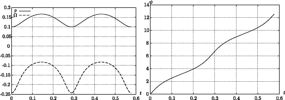

  

  Functions ρ(t), ψ(t) and Ω(t)

• 1.2. For r=σ (the center of the body is on the circle r=σ), the system of equations (35) has a family of fixed points lying on the straight line ψ=ψ _∗=π+φ ₀. The phase trajectories of the system for φ ₀=π and various values of the integral G are shown in Fig. 7.

  Fig. 7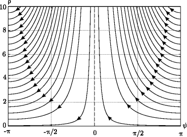

  

  Phase trajectories of the system (35) for φ ₀=π and $\frac {r}{\sigma } = 1$

It can be seen from Fig. 7 that the phase variable ρ increases infinitely in a neighborhood of the straight line ψ=ψ _∗.

Let us examine the attainability of a fixed point. To do so, we linearize equation (57) in its neighborhood

$$ \dot{\psi} = \frac{r^{2} \sin^{2} \psi_{*}}{m G} (\psi - \psi_{*})^{2}. $$

(58)

Let us integrate (58) on the interval [ψ _∗−ε, ψ _∗)

$$ t \frac{r^{2} \sin^{2}\psi_{*}}{mG} = \frac{1}{\varepsilon} - \lim_{\psi \rightarrow \psi_{*}}\frac{1}{\psi - \psi_{*}} = \infty. $$

(59)

Consequently, the phase trajectories approach the straight line ψ=ψ _∗ in infinite time. Thus, for $\sin \varphi _{0} = 0$ and r=σ, a partial stabilization can be performed only in finite time.

• 1.3. For r>σ (the center of the body is outside the circle r=σ), equation (57) admits particular steady-state solutions

  $$ \psi^{*}_{\pm} = \left\{\begin{array}{ll} \pm \left(\pi - \arccos \frac{\sigma}{r} \right), & \varphi_{0} = 0,\\ \pm \arccos \frac{\sigma}{r}, & \varphi_{0} = \pi. \end{array}\right. $$

  (60)

  The phase trajectories of the system on the plane (ρ, ψ) for various values of the integral G and the parameter values r=1, σ=0.5 are shown in Fig. 8.

  Fig. 8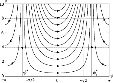

  

  Phase trajectories of the system (35) for $\sin \varphi _{0} = 0$ and $\frac {r}{\sigma } > 1$

It can be seen from Fig. 8 that the phase trajectories approach the vertical asymptotes $\psi = \psi ^{*}_{\pm }$, hence, as time goes on, $\rho \rightarrow +\infty$. Performing the same analysis as in the previous case, we can show that the value ψ=ψ ₊ is reached in infinite time. Thus, for $\sin \varphi _{0} = 0$ and r>σ, a partial stabilization can be performed only in finite time.

• 2. Consider a more general case for which the line of motion of the internal mass is such that $\sin \varphi _{0} \neq 0$. In this case, the integral (55) can be written as

  $$ G = \rho (r \cos \psi + \overline{\sigma} ) \exp \left(- \sigma \sin \varphi_{0} \int \frac{d\psi}{r \cos \psi + \overline{\sigma}} \right)=\text{const}\,,\quad \overline{\sigma} = \sigma \cos \varphi_{0}. $$

  (61)

  The exact form of the integral (61) depends on the relationship between r and $\sigma \vert \cos \varphi _{0} \vert$. The equality $r = \sigma \vert \cos \varphi _{0} \vert$ defines the circle with the center at the point $\left (\frac {\zeta }{\lambda },\, -\frac {\chi }{\lambda } \right )$ and radius $\frac {\sqrt {\chi ^{2} + \zeta ^{2}}}{\lambda } \vert \cos \varphi _{0} \vert$.

• 2.1. For $r < \sigma \vert \cos \varphi _{0} \vert$ (the center of the body is inside the circle $r = \sigma \vert \cos \varphi _{0} \vert$), the integral (61) is not unique and can be represented as

  $$\begin{array}{@{}rcl@{}} \overline{G}&=&\frac{G}{r} = \rho (\cos \psi + \kappa ) \\ &&\times \exp \left(- \frac{2 \kappa \tan \varphi_{0}}{\sqrt{\kappa^{2} - 1}} \left(\arctan \left(\frac{\sqrt{\kappa^{2} - 1}}{\kappa + 1} \tan \frac{\psi}{2}\right) + \left[ \frac{\psi + \pi}{2\pi}\right] \pi \right) \right)=\text{const},\\ \end{array} $$

  (62)

  where $\kappa = \frac {\overline {\sigma }}{r}$, |κ|>1, ψ∈[−π, π).

The trajectories of the system (35) fill everywhere densely the plane (ρ, ψ). Depending on the relationship between the parameters r, σ, and φ ₀, two types of phase portraits are possible (see Fig. 9).

Fig. 9

Phase portraits of the system for σ=1.5, φ ₀=0.1. a) r=0.1, b) r=1

Indeed, the right-hand side of the second equation of (35) is nonnegative (nonpositive) for $\frac {\sigma \vert \sin \varphi _{0} \vert }{r} \geqslant 1$. This means nondecrease (nonincrease) of the function ρ (see Fig. 9a). Otherwise, the sign $\dot {\rho }$ changes twice in one period of the variable ψ, and the system trajectories have extrema (see Fig. 9b).

According to the first equation of (35), the function ψ(t) is monotonous, since the right-hand side of the equation is sign-definite by virtue of the condition $r < \sigma \vert \cos \psi _{0} \vert$. Using the integral (62), we estimate the change of ρ for one period of the variable ψ∈[−π, π)

$$ {\Delta} \rho = \rho_{0} \left(\exp \left(\frac{2 \pi \kappa \tan \varphi_{0}}{\sqrt{\kappa^{2} - 1}} \right) - 1 \right). $$

(63)

It can be seen from (63) that the increment Δρ of the phase variable ρ is directly proportional to the value ρ ₀=ρ| _ψ=−π . Moreover, $\text {sign} {\Delta } \rho = \text {sign } \tan \varphi _{0}$. It is easy to show that for N periods the increment is

$$ {\Delta} \rho_{N} = \rho_{0} \left(\exp \left(\frac{2 N \pi \kappa \tan \varphi_{0}}{\sqrt{\kappa^{2} - 1}} \right) - 1 \right). $$

(64)

That is, the increment depends exponentially on the number of periods N. Thus, despite the existence of two types of phase portraits, the phase variable ρ increases on an average if $\tan \varphi _{0} > 0$ and decreases on an average if $\tan \varphi _{0} < 0$.

According to (36), as ρ decreases infinitely, ${\Omega } \rightarrow \infty$. Thus, if the condition $r < \sigma \vert \cos \varphi _{0} \vert$ is satisfied, either ρ or Ω increases indefinitely, depending on the value of φ ₀. Thus, for $\sin \varphi _{0} \neq 0$ and $r = \sigma \vert \cos \varphi _{0} \vert$, a partial stabilization can be performed only in finite time.

• 2.2. For $r > \sigma \vert \cos \varphi _{0} \vert$ (the center of the body is outside the circle $r = \sigma \vert \cos \varphi _{0} \vert$), the integral (61) can be written as

  $$ \overline{G} = - \rho \frac{\text{sign}\, (\tau_{+}(\psi) \tau_{-}(\psi) )}{1 + \tan^{2} \frac{\psi}{2}} \vert \tau_{-} (\psi) \vert^{\delta + 1} \vert \tau_{+} (\psi) \vert^{1-\delta}, $$

  (65)
  $$\begin{array}{c} \delta = \frac{\kappa \tan \varphi_{0}}{\sqrt{1 - \kappa^{2}}},\quad \tau_{\pm}(\psi) = \sqrt{ 1 - \kappa} \tan \frac{\psi}{2} \pm \sqrt{ 1 + \kappa}. \end{array} $$

  Consider the values $\psi _{\pm } = \mp 2 \arctan \sqrt {\frac {1 + \kappa }{1 - \kappa }}$, which are zeros of the functions τ _±(ψ). It is seen from (65) that the behavior of the system (35) in a neighborhood of the lines ψ=ψ _± can change depending on the parameter δ. For the values δ<0, three possible types of phase portraits are shown in Fig. 10.

  Fig. 10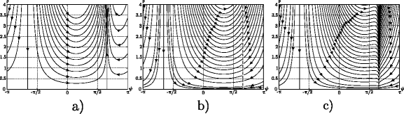

  

  a) δ=−0.5, b) δ=−1, c) δ=−1.1

Remark B.1

By virtue of the symmetry (54), the phase portrait for some δ=−δ ₀<0 can be obtained by a mirror reflection of the phase portrait for δ=δ ₀ relative to ψ=0 and by changing the direction of motion along the trajectories.

• 2.2.1. If |δ|<1, the phase variable ρ infinitely increases near ψ _±. The asymptotes ψ=ψ _± are always separated from each other regardless of the relationship between the parameters r, σ, and φ ₀. Hence, the qualitative behavior of the system trajectories on the plane (ρ, ψ) (see Fig. 10a) is also independent of the relationships between these parameters and is the same as the behavior considered in the case $\sin \varphi _{0} = 0$, r>σ (see Fig. 8). Thus, for $\sin \varphi _{0} \neq 0$ and $r < \sigma \vert \cos \varphi _{0} \vert$, a partial stabilization can be performed only in finite time.

• 2.2.2. The condition |δ|=1 is equivalent to the equality r=σ. In this case, the right-hand sides of equations (35) vanish simultaneously for ψ=π+φ ₀. When δ=−1, the asymptote ψ=ψ ₋ disappears, and its place is taken by a family of fixed points; there are no qualitative changes in a neighborhood of the asymptote ψ=ψ ₊ (see Fig. 10b). Similarly, when δ=1, the lines ψ=ψ ₊ correspond to a family of fixed points and ψ=ψ ₋ is an asymptote. To perform a stability analysis of these fixed points, we represent the first equation of (35) as

  $$ m \rho \dot{\psi} = -\frac{r}{1 + \tan^{2} \frac{\psi}{2}} \tau_{+} (\psi)\tau_{-} (\psi) . $$

  (66)

  Let us analyze the stability of the family of fixed points ψ=ψ ₋ for δ=−1. For this purpose, we linearize (66) in a neighborhood of ψ=ψ ₋

  $$ m \rho \dot{\Delta \psi} = - \frac{r}{1 + \tan^{2} \frac{\psi_{-}}{2}} \tau_{+}(\psi_{-}) \frac{\sqrt{1 - \kappa}}{2 \cos^{2} \frac{\psi_{-}}{2}} {\Delta} \psi, \quad \psi = \psi_{-} + {\Delta} \psi . $$

  (67)

  Since the coefficient of Δψ is negative, the fixed points of the family ψ=ψ ₋ are stable. In a similar way, it can be shown that the fixed points of the family ψ=ψ ₊ are unstable for δ=1. Since $\text {sign} \delta = \text {sign} \tan \varphi _{0}$, the system has the above family of stable fixed points for $\tan \varphi _{0} <0$, and the family of unstable fixed points for $\tan \varphi _{0} > 0$. Thus, a partial stabilization is possible in infinite time when $\sin \varphi _{0} \neq 0$, $r > \sigma \vert \cos \varphi _{0} \vert$ and δ=−1.

• 2.2.3. Consider the behavior of the system for |δ|>1. The phase portrait corresponding to δ<−1 is shown in Fig. 10c. The behavior in a neighborhood of the straight line ψ=ψ ₊ does not change qualitatively. In contrast to the cases considered above, the line ψ=ψ ₋ becomes a discontinuity of the integral $\overline {G}$. Note that due to equation (66)$\dot {\psi } > 0$ for ψ∈(ψ ₊, ψ ₋) and $\dot {\psi } < 0$ for $\psi \in [-\pi / 2,\, \psi _{+}) \cup (\psi _{-},\, \pi / 2]$. Thus, all trajectories of (35) tend to the point ψ=ψ ₋, ρ=0 on a given level set of the integral $\overline {G}$.

  The point ψ=ψ ₋, ρ=0 is the singular point of (35). This singularity may be due to either the choice of polar coordinates or the existence of an essential singular point in the system. In order to define the type of singularity, it is necessary to examine the value of the limit $\lim \limits _{\rho \rightarrow 0} \dot {\rho }$ depending on ψ. This analysis for the system considered shows that the point ψ=ψ ₋, ρ=0 is an essential singular point and all trajectories of the system converge to it.

Consider the attainability of the point ψ=ψ ₋, ρ=0 in finite/infinite time. Let us eliminate ρ from the first equation of (35) using the integral (65)

$$ \dot{\psi} = \frac{1}{m G} \frac{1}{\left(1+\tan^{2} \frac{\psi}{2}\right)^{2}} \vert \tau_{+} (\psi) \vert^{2-\delta} \vert \tau_{-} (\psi) \vert^{2+\delta} . $$

(68)

Equation (68) can be approximated by

$$ \dot{\psi} = {\Lambda} (\psi - \psi_{-})^{2 + \delta} $$

(69)

using the Taylor series expansion of the function τ ₋(ψ) in a neighborhood of ψ=ψ ₋. Without loss of generality, we set ψ−ψ ₋>0. Since 2+δ<1, the solution of (69) is the following power function:

$$ \psi = \psi_{-} + (-(1 + \delta) ({\Lambda} t + C))^{-1 / (\delta + 1)}, $$

(70)

whence it is clear that the line ψ=ψ ₋ is attained in finite time.

Let us consider the behavior of the angular velocity Ω as the line ψ=ψ ₋ is approached. Expression (36) can be written as

$$ {\Omega} = \frac{1}{I_{r}} \left(C_{xy} - (m \rho^{2} + \overline{b}) \dot{\psi} \right). $$

(71)

It is seen from (69) and (71) that for δ∈(−2, −1) the derivative $\dot {\psi }$ tends to zero as ψ=ψ ₋ is approached, hence, ${\Omega } \rightarrow \frac {C_{xy}}{I_{r}}$. If δ=−2, then $\dot {\psi } = {\Lambda }$, hence, ${\Omega } \rightarrow \frac {C_{xy} - \overline {b} {\Lambda }}{I_{r}}$. If δ<−2, then $\dot {\psi } \rightarrow \infty$, hence, ${\Omega } \rightarrow \infty$. Thus, a partial stabilization is possible in finite time for $\sin \varphi _{0} \neq 0$, $r > \sigma \vert \cos \varphi _{0} \vert$ and |δ|>1. □

References

Agrachev AA, Sachkov Y. Control theory from the geometric viewpoint: Springer Science & Business Media; 2004.
Arnold VI. Mathematical methods of classical mechanics: Springer Science & Business Media; 1989.
Bonnard B. Contrôlabilité des systèmes nonlinéaires. C R Acad Sci Paris Sér 1 1981;292:535–537.
Bonnard B, trajectories Chyba M., Vol. 40. Their role in control theory Singular: Springer Science & Business Media; 2003.
Bolotin SV. The problem of optimal control of a Chaplygin ball by internal rotors. Rus J Nonlin Dyn 2012;8(4):837–852. Russian.
Borisov AV, Mamaev IS. On the motion of a heavy rigid body in an ideal fluid with circulation. CHAOS 2006;16(1):013118. (7 pages).
Borisov AV, Kilin AA, Mamaev IS. How to control chaplygin’s sphere using rotors. Regul Chaotic Dyn 2012;17(3–4):258–272.
Borisov AV, Kilin AA, Mamaev IS. How to control the chaplygin ball using rotors. II. Regul Chaotic Dyn 2013;18(1–2):144–158.
Borisov AV, Kilin AA, Mamaev IS. Dynamics and Control of an Omniwheel Vehicle. Regul Chaotic Dyn 2015;20(2):153–172.
Borisov AV, Kozlov VV, Mamaev IS. Asymptotic stability and associated problems of failing rigid body. Regul Chaotic Dyn 2007;12(5):531–565.
Borisov AV, Mamaev IS, Kilin AA, Bizyaev IA. Qualitative Analysis of the Dynamics of a Wheeled Vehicle. Regul Chaotic Dyn 2015;20(6):739–751.
Chaplygin S. On the influence of a plane-parallel flow of air on moving through it a cylindrical wing. Tr Cent Aerohydr Inst 1926;19:300–382.
Childress S, Spagnolie SE, Tokieda T. A bug on a raft: recoil locomotion in a viscous fluid. J Fluid Mech 2011;669:527–556.
Chow W, Über L. Systeme von linearen partiellen Differentialgleichungen erster Ordnung. Math Ann 1939;117(1):98–105.
Chyba M, Leonard NE, Sontag ED. Optimality for underwater vehicles. IEEE 1998,2001;5:4204–4209.
Chyba M, Leonard NE, Sontag ED. Singular trajectories in multi-input time-optimal problems: application to controlled mechanical systems. J Dyn Control Syst 2003;9(1):103–129.
Crouch PE. Spacecraft attitude control and stabilization: applications of geometric control theory to rigid body models. IEEE Trans Autom Control 1984;29(4):321–331.
Ivanov AP. On the control of a robot ball using two omniwheels. Regul Chaotic Dyn 2015;20(4):441–448.
Jurdjevic V. Geometric control theory. Cambridge: University Press; 1997.
Karavaev YL, Kilin AA. The Dynamics and Control of a Spherical Robot with an Internal Omniwheel Platform. Regul Chaotic Dyn 2015;20(2):134–152.
Kilin AA, Vetchanin EV. The contol of the motion through an ideal fluid of a rigid body by means of two moving masses. Nelin Dinam 2015;11(4):633–645. (in Russian).
Kirchhoff G., Hensel K. Vorlesungen über mathematische Physik. Mechanik. Leipzig: BG Teubner; 1874, p. 489.
Kozlov VV, Onishchenko DA. The motion in a perfect fluid of a body containing a moving point mass. J Appl Math Mech 2003;67(4):553–564.
Kozlov VV, Ramodanov S. On the motion of a variable body through an ideal fluid. PMM 2001;65(Vyp. 4):529–601.
Lamb H. Hydrodynamics. New York: Dover; 1945, p. 728.
Leonard NE, Marsden JE. Stability and drift of underwater vehicle dynamics: mechanical systems with rigid motion symmetry. Phys D: Nonlinear Phenom 1997;105 (1):130–162.
Leonard NE. Stability of a bottom-heavy underwater vehicle. Automatica 1997; 33(3):331–346.
Murray RM, Sastry SS. Nonholonomic motion planning: steering using sinusoids. IEEE Trans Autom Control 1993;38(5):700–716.
Ramodanov SM, Tenenev VA, Treschev DV. Self-propulsion of a body with rigid surface and variable coefficient of lift in a perfect fluid. Regul Chaotic Dyn 2012;17 (6):547–558.
Rashevskii PK. About connecting two points of complete non-holonomic space by admissible curve (in Russian). Uch Zapiski Ped Inst Libknexta;2:83–94.
Steklov VA. On the motion of a rigid body through a fluid. Article 1. Soob Khark Mat Obsch 1891;2(5–6):C.209–235.
Svinin M, Morinaga A, Yamamoto M. On the dynamic model and motion planning for a class of spherical rolling robots. IEEE Int Conf Robot Autom 2012;2012: 3226–3231.
Vankerschaver J, Kanso E, Marsden JE. The dynamics of a rigid body in potential flow with circulation. Regul Chaotic Dyn 2010;15(4-5):606–629.
Vetchanin EV, Kilin AA. Free and controlled motion of a body with moving internal mass though a fluid in the presence of circulation around the body. Dokl Phys 2016;466(3):293–297.
Vetchanin EV, Mamaev IS, Tenenev VA. The self-propulsion of a body with moving internal masses in a viscous fluid. Regul Chaotic Dyn 2013;18(1-2):100–117.
Woolsey CA, Leonard NE. Stabilizing underwater vehicle motion using internal rotors. Automatica 2002;38(12):2053–2062.
Acknowledgments
The authors thank A.V. Borisov and I.S. Mamaev for fruitful discussions. The work of E.V. Vetchanin was supported by the RFBR grant 15-08-09093-a. The work of A.A. Kilin was supported by the RFBR grant 14-01-00395-a.
Author information
Authors and Affiliations
Corresponding author