
Abstract
We present an operationally motivated treatment of quantum reference frames in the setting that the frame is a covariant positive operator valued measure (POVM) on a finite homogeneous space, generalising the principal homogeneous spaces studied in previous work. We focus on the case that the reference observable is the canonical covariant projection valued measure on the given space, and show that this gives rise to a rank-one covariant POVM on the group, which can be seen as a system of coherent states.
1 Introduction
In the orthodox treatment of quantum theory, there is an implicit reliance on background (external) reference frames which underpin the description of states and observables, and whose interpretation is rooted in classical physics. The topic of quantum reference frames (QRFs) seeks to provide a theory in which reference frames are viewed as quantum physical systems and treated internally, i.e. as an explicit part of the theoretical description of the quantum physical world. Though the idea can be traced back as far as 1946 [1], the main catalyst for the modern ideas can be found in an exchange regarding the nature of superselection rules in the late 60’s [2, 3], and appears in a more definitive form in the 80’s [4]. This subject continues to inspire both pure and applied research, and a variety of formulations now exist; broadly these split into four categories: that motivated by ideas in quantum information (largely summarised in [5]; see [6] for some recent work), that motivated by gauge theory and Dirac quantisation of constrained systems, known as the perspective-neutral approach [7,8,9,10], that founded on a direct description of frame transformations [11, 12], and that closer to operational ideas in quantum mechanics and quantum measurement theory [13,14,15,16,17,18,19,20].
The present contribution follows the latter, ‘operational’, approach [20, 21]. Though (symmetry) groups appear in essentially all work on QRFs, the role they play differs. In the operational approach the basic physical principle is that what can be measured is invariant under a unitary representation of the given group. For single systems considered in isolation, this may leave very few observables, but for compound systems there are generally many non-trivial invariants. Here, we typically consider a system \(\mathcal {S}\) and a reference frame \(\mathcal {R}\), represented, respectively, by Hilbert spaces \(\mathcal {H}_{\mathcal {S}}\) and \(\mathcal {H}_{\mathcal {R}}\), with their given state spaces and observables. Only invariant observables in \(\mathcal {H}_{\mathcal {S}}\otimes \mathcal {H}_{\mathcal {R}}\) can be measured. Among these are those which can be interpreted as ‘system relative to frame’, which are obtained through a relativisation map, which explicitly introduces the quantum reference frame into the description, denoted by \(\yen\) in previous works (e.g. [15]).
The \(\yen\) map is constructed so as to give rise to positive operator valued measures (POVMs) invariant under a tensor product unitary representation \(U_{\mathcal {S}}\otimes U_{\mathcal {R}}\) of a given locally compact group G, given explicitly as
Here, \(\textsf{E}\)—the frame observable—is a covariant POVM whose domain is the Borel sets of G, i.e., for any \(X \in \mathcal {B}(G)\), \(U_{\mathcal {R}}(g)\textsf{E}(X)U_{\mathcal {R}}(g)^* = \textsf{E}(g.X)\), and \(\textsf{A}\) is a POVM with arbitrary value space containing (measurable) \(\Omega\). The \(\yen\) map is completely positive and normal, unit and adjoint preserving, and takes values in the (\(G-\)) invariant algebra \(B(\mathcal {H}_{\mathcal {S}}\otimes \mathcal {H}_{\mathcal {R}})^G\). \(\yen\) is understood as taking arbitrary quantities to their corresponding relative observables [15, 20]. For instance, \(\yen\) produces relative position, phase, angle and time [18] observables from their ‘absolute’ versions. If \(\textsf{E}\) admits a state which is arbitrarily well localised at the identity in G (which follows from a technical condition known as the norm-1 property [22]), it can be shown that \(\textsf{A}\) and \(\yen \circ \textsf{A}\) can be made arbitrarily probabilistically close, pointing to an equivalence between the descriptions with internal and externalised frame. Conversely, if \(\textsf{E}\) is not well localisable (i.e., there are no states which give localisation probability close to one on ‘small’ sets), there are distributions given by \(\textsf{A}\) which cannot be captured at the invariant level. (See [15, 17] for further details). From here we conclude that for the ordinary framework of quantum mechanics (states, observables, probabilities) describing a system \(\mathcal {S}\) to approximate well the relative description (states, invariant observables, probabilities) of \(\mathcal {S}\) and \(\mathcal {R}\) combined, some classical-like features of the reference are needed.
Much of the literature on quantum reference frames assumes that the system \(\mathcal {R}\) comes equipped with the left regular representation of G, namely that \(\mathcal {H}_{\mathcal {R}}\) is chosen as \(L^2(G)\), and in the operational framework that \(\textsf{E}\) is given as the unique covariant projection valued measure (PVM). This means in particular that the value space of the frame observable is chosen (as a space) to be G itself. In physical terms, this says roughly that the configuration space of the frame is the group. However, there are many physical scenarios where this is too restrictive, and the physics dictates that a group acts on a homogeneous space rather than on itself. A standard example is the Poincaré group \(\mathcal {P}\) acting on Minkowski space \(\mathcal {M}\); here a quantum reference frame consists of a POVM on \(\mathcal {M}\) which is covariant under the given representation of \(\mathcal {P}\). In other words, G as above should be replaced by some homogeneous G-space X on which the action of G is (possibly) not free, and the frame observable \(\textsf{E}\) should therefore be defined on this space. This may arise from e.g. limitations on the availability of a physical frame, or for fundamental reasons. For instance, a frame may be so basic that it is only capable of resolving whether a particle is left or right of some chosen point, and therefore the value space of the frame observable is two-valued. Mathematically, such a move requires a significant update of (1), and in the present work we provide this generalisation for the case that G and X are finite, in order to bring out some of the key physical observations without recourse to the full machinery of locally compact groups.
The presence of a non-trivial stabiliser/isotropy subgroup necessitates a re-appraisal of the physics of quantum reference frames in contrast to [13,14,15,16,17,18,19], and is the subject of this paper. Our work differs from that of [10], in which a quantum frame is given by a system of coherent states \(S=\{\eta _g ~|~g \in G\}\) and an incomplete frame corresponds to the presence of a non-trivial subgroup of G which stabilises \(\eta _{e}\). However, in the setting that the frame observable is the canonical covariant PVM on X acting in \(L^2(X)\), we will show that this induces a rank-1 POVM on G which can be interpreted as a system of coherent states. We see that the presence of the stabiliser subgroup, through the relativisation and restriction procedures “enforces" its symmetry back on \(\mathcal {S}\), in direct analogy to the findings of [10], thereby providing some first connections between the operational and perspective-neutral approaches.
2 Preliminaries
The standard objects in quantum theory are presumed [23]: observables are identified with positive operator valued measures (POVMs) and states by positive (trace class) operators with unit trace. Sharp observables are identified among all observables as the projection valued measures (PVMs), and hence also to the corresponding self-adjoint operator. In addition, we consider a finite set X which transforms under the action of a finite group G and quantum reference frames (‘frame observables’) are constructed as covariant (under a unitary Hilbert space representation of G) POVMs on X, with special attention given to the canonical PVM on X. After introducing these covariant objects, we consider the probability measures on X given by a frame observable and a state, focussing on two key cases: the invariant states, which as we will see later are maximally bad frames, and the localised states, which are maximally informative.
2.1 Setup
Throughout the rest of this paper, G denotes a finite group with identity \(e \in G\), X a finite set with a transitive left G-action \(\alpha :G \times X \rightarrow X\); we write \(g \cdot x\) for \(\alpha (g,x)\), and \(U_{\mathcal {S}}\) is a unitary representation of G in a Hilbert space \(\mathcal {H}_{\mathcal {S}}\) representing some quantum system \(\mathcal {S}\) (which is arbitrary). Unless stated otherwise we fix \(\mathcal {H}_{\mathcal {R}}:= L^2(X)\) as the Hilbert space of complex functions on X, and \(B(L^2(X))\) the space of linear operators \(L^2(X) \rightarrow L^2(X)\). For \(x \in X\) we denote by \(G_{x} := \{ g \in G \; | \; g \cdot x = x \}\) the stabiliser of x. Note that \(G_{g \cdot x} = g G_{x} g^{-1}\). The map \(G/G_{x} \rightarrow X\), \(gG_{x} \mapsto g \cdot x\) is a G-equivariant bijection. We set \(n := |X|\), which is equal to \(|G/G_{x}|\) and therefore also to the dimension of \(L^2(X)\).
By \(U_{R}\) we denote the unitary representation of G on \(L^2(X)\) defined by \((U_{\mathcal {R}}(g)f)(x) = f(g^{-1} \cdot x)\) for \(f \in L^2(X)\) and \(g \in G\) (where it is not ambiguous, we will also write \(g \cdot f\) for \(U_{\mathcal {R}}(g)f\)). Note that if \(\delta _{x}\) is the indicator function of \(x \in X\) then \(g \cdot \delta _{x} = \delta _{g \cdot x}\). The state \(\delta _{x}\) may be written \(|x\rangle\) and the corresponding rank-1 projection \(P_x\) by \(|x\rangle \langle x|\). Fixing \(x \in X\) and setting \(H:=G_x\) identifies X with G/H and \(L^2(X)\) with the induced representation \(L^{2}(G/H) = \textrm{Ind}_{H}^{G} \mathbb {C}\). (Since the stabilisers of different x are conjugate, the corresponding induced representations are isomorphic.) Setting \(X=G\) with the action given by the group multiplication yields the left regular representation of G.
For \(x \in X\), with \(|x\rangle \langle x| \equiv P_{x} \in B(L^2(X))\) the projection onto the subspace spanned by \(\delta _{x}\), we denote by P the projection valued measure (PVM) defined by
extended by additivity to subsets of X. The PVM P is equivariant/covariant with respect to the actions of G on X and on \(B(L^2(X))\), i.e. \(P_{g \cdot x} = U_{R}(g) P_{x} U_{R}(g)^* = g \cdot P_{x}\). (The pair \((P,U_{R})\) corresponds to the standard representation of the crossed product \(C(X) \rtimes G\) on \(L^{2}(X)\) [24].) We let G act on \(B(\mathcal {H}_{\mathcal {S}})\) and on \(B(L^2(X))\) by conjugation, so that \(g \cdot A = U_{\mathcal {S}}(g) A U_{\mathcal {S}}(g)^*\) for \(A \in B(\mathcal {H}_{\mathcal {S}})\) and \(g \in G\), and similarly for \(B \in B(L^2(X))\). G acts on \(B(\mathcal {H}_{\mathcal {S}})\otimes B(L^2(X))\) diagonally, i.e., by conjugation by \(U_{\mathcal {S}}(g)\otimes U_{\mathcal {R}}(g)\). The triple \((U_\mathcal {R},P,L^2(X))\) is understood as a quantum reference frame, and P the frame observable.
Remark 2.1
We work primarily in the setting that the frame is given as above. However, there is a generalisation in which P is replaced by a covariant POVM E, and \(L^2(X)\) can be any Hilbert space in which the covariant POVM can be constructed, e.g. it can by smaller than \(L^2(X)\).
2.2 States and Probabilities on the Frame
Pure states of the form \(P_{x}\) corresponding to the function \(\delta _{x}\) are understood as being localised at the corresponding point in X; this is motivated through the localisation of the probability measure to which we will soon turn. We note also that these states are not G-invariant unless G acts trivially on X. The space of G-invariant vectors \(L^2(X)^{G}\) in \(L^2(X)\) is one dimensional and spanned by the constant function \(\varvec{1}\), since
by Frobenius reciprocity (e.g. [25]). The corresponding state \(P_{\varvec{1}}\) is obviously G-invariant.
More generally, invariant pure states correspond to vectors that are contained in one-dimensional subrepresentations, because if \(\phi \in L^2(X)\) then \(U_{\mathcal {R}}(g) P_{\phi } U_{\mathcal {R}}(g)^* = P_{\phi }\) if and only if \(U_{\mathcal {R}}(g) \phi = \lambda \phi\) for some \(\lambda \in S^{1}\) (the set of complex numbers of modulus 1). Equivalently, for each \(x \in X\) and \(g \in G\)
for some \(\lambda \in S^{1}\). Non-zero vectors of this type correspond to one dimensional subrepresentations of \(L^2(X)\). If \(\mathbb {C}_{\chi }\) is such a representation, where \(g \cdot v=\chi (g)v\) for \(\chi :G \rightarrow \mathbb {C}^{\times }\), then
so that invariant pure states correspond to one dimensional representations of G that are trivial when restricted to H. There always exists an invariant mixed state by the finite dimensionality of \(L^2(X)\), given by \(\frac{1}{n} \mathbb {I}\) (where \(n = |X| = \textrm{dim}~ L^2(X)\)).
Probability measures/distributions are given by the usual trace formula. For a POVM E and a state \(\rho\),
is a probability distribution on X; the corresponding measure is obtained through the additivity of E. If \(\rho\) is a rank one projection defined by the unit vector \(\phi\), we write \(p^E_{\phi }(x)\) for the distribution. A state \(\rho\) is called localised at \(x\in X\) with respect to E if \(p^E_{\rho }(x)=1\), i.e., if upon measurement of E, the outcome x is found with probabilistic certainty. In case \(X=G\), the POVM E paired with some state gives a probabilistic orientation assignment on G.
In general POVMs do not share the localisability properties of PVMs. For any PVM Q on X, given a projection \(Q_x\) there is a state \(\rho\) for which \(\text {tr}\left[ Q_x\rho \right] =1\) - simply take (for example) \(\rho\) to be the projection onto any unit vector in the range of \(Q_x\). For a POVM E on X it may be the case that there is no such state; we will encounter such an example in Subsec. 3.3 for a POVM on G corresponding to a system of coherent states. However, we recall that a POVM E satisfies the norm-1 property if each \(E(x)\ne 0\) has \(||E(x)||=1\) (\(||\cdot ||\) denotes the operator norm). The following proposition characterises POVMs with the localisability properties of PVMs, i.e., there is a state for which \(\text {tr}\left[ E(x)\rho \right] =1\). This unit probability can also be interpreted as E possessing the property associated with x with probabilistic certainty in the state \(\rho\).
Proposition 2.2
The following are equivalent:
-
1.
E satisfies the norm-1 property;
-
2.
For each \(E(x) \ne 0\) there is a state \(\rho\) such that \(\text {tr}\left[ E(x)\rho \right] =1\);
-
3.
For each \(E(x) \ne 0\) there is a pure state \(\rho\) such that \(\text {tr}\left[ E(x)\rho \right] =1\).
The proof follows from the spectral radius formula and the finite dimensionality of the Hilbert space.
Returning to the canonical PVM P, we conclude by observing that the distribution for P and any G-invariant pure state is uniform, equal to that given by the state \(\frac{1}{n} \mathbb {I}\): If \(P_{\phi }\) is G-invariant, then by (2) the function \(|\phi (x)|^2\) is constant, with value \(\frac{1}{n}\) if \(\phi\) is normalised. We have that \(p^P_{\phi } : X \rightarrow \mathbb {R}^{\ge 0}\) is equal to \(x \mapsto \textrm{tr} \left( P_{x} P_{\phi } \right) = \langle \phi , P_{x} \phi \rangle = | \phi (x) |^2 = \frac{1}{n}\), and therefore \(p^P_{\phi } = p^P_{\frac{1}{n} \mathbb {I}}\).
3 Relativisation and Restriction
A quantum system \(\mathcal {S}\) represented by a Hilbert space \(\mathcal {H}_{\mathcal {S}}\) is combined with a quantum reference frame \(\mathcal {R}\) with Hilbert space \(L^2(X)\). Relative observables on \(\mathcal {H}_{\mathcal {S}}\otimes L^2(X)\) are constructed through a generalisation to a finite homogeneous space of the relativisation (\(\yen\)) mapping (1). We provide a family of such maps—one for each \(x\in X\)—and for these to be well defined the domain must be \(G_x\) invariant. As we shall see, the presence of the non-trivial stabiliser means that only \(G_x\)-invariant observables of \(\mathcal {S}\) can be ‘measured’, or more accurately, no G-invariant observable of system plus reference can ever generate statistics corresponding to non-\(G_x\)-invariant observables of \(\mathcal {S}\). Therefore if \(G_x\) is non-trivial we view the frame as incomplete, in line with other usage in the literature (e.g. [10]).
3.1 The \(\yen\) Map on a Homogeneous Space
Proposition 3.1
For \(x \in X\) the map
is a unit preserving, injective C*-algebra homomorphism, where the sum is over a set of representatives of the left cosets of \(G_{x}\) in G.
Proof
First note that the right hand side of (4) well defined because A is \(G_{x}\)-invariant: if \(g,g'\) are both representatives of a coset \(gG_x = g'G_x\), then \(g = g'h\) for some \(h \in G_x\), and
where \(g'h \cdot x = g' \cdot x\) because \(h \in G_{x}\). If \(k \in G\) then
which shows that \(\yen _x(A)\) is G-invariant. Fix representatives \(g_1=e, \dots , g_n\) of the left cosets of \(G_{x}\). Then the ordered basis \(\delta _{g_i \cdot x}\), \(1 \le i \le n\) of \(L^{2}(X)\) identifies \(B(L^2(X))\) with \(\textrm{M}_{n}(\mathbb {C})\) and \(B(\mathcal {H}_{\mathcal {S}})\otimes \textrm{M}_{n}(\mathbb {C})\) with \(\textrm{M}_{n}(B(\mathcal {H}_{\mathcal {S}}))\). Under this identification \(\yen _x(A)\) is equal to the diagonal matrix
from which it follows that the map \(\yen _x\) is a unit preserving, injective C*-algebra homomorphism. \(\square\)
Note that the right hand side of (4) can be written \(\frac{1}{|G_x|}\sum _{g \in G}U_{\mathcal {S}}(g)AU_{\mathcal {S}}(g)^*\otimes P_{g.x}\). Observables in the image of this map are understood as relative - relating system and frame. They correspond in this setting to the relational Dirac observables described in e.g. [26]. Note also that the properties of the map \(\yen _x\) established in Prop. 3.1 can be derived from Prop. 3.8 and the properties of \(\yen\) as given in [15].
Remark 3.2
Replacing \(B(L^2(X))\) by any \(B(\mathcal {H}_{\mathcal {R}})\) for which a covariant POVM E on X may be constructed yields a well defined linear map
However, if E is not projection-valued, the injectivity and homomorphism properties are lost; note also that E may not have rank-1 effects. The map is however completely positive. In such a case the image of the relativisation map is still understood as corresponding to relative observables, and indeed such a frame may be needed in certain cases, for fundamental or practical reasons (e.g., most time observables are unsharp - see [18]).
Remark 3.3
In case \(X=G\) there are isomorphisms giving \(B(\mathcal {H}_{\mathcal {S}}) \rtimes G \cong (B(\mathcal {H}_{\mathcal {S}}) \otimes B(L^2(G)))^G \cong B(\mathcal {H}_{\mathcal {S}}) \otimes B(L^2(G))^G\); under the first isomorphism (given in e.g. [27]) \(\yen _e\) corresponds exactly to the natural inclusion of \(B(\mathcal {H}_{\mathcal {S}})\) into the crossed product algebra \(B(\mathcal {H}_{\mathcal {S}}) \rtimes G\). We remark that here \(B(L^2(G))^G \cong C^*(G)\) and the isomorphism \(B(\mathcal {H}_{\mathcal {S}}) \rtimes G \cong B(\mathcal {H}_{\mathcal {S}}) \otimes C^*(G)\) is given in e.g. [28] Ch. 2, App. C. The second isomorphism shows that the full algebra of invariants is isomorphic to the original algebra tensored with the invariant algebra of \(L^2(G)\), giving a novel description of the invariant algebra, suggesting that the “relational information" can be completely factored into one component of the tensor product. This is yet to be fully understood in this context.
We finally comment that we can replace G with G/H and \(B(\mathcal {H}_{\mathcal {S}})\) with a von Neumann algebra \(\mathcal {A}\) to find \(\mathcal {H}(G,H,\mathcal {A},\alpha ) \cong (\mathcal {A} \otimes B(L^2(G/H)))^G\); here \(\mathcal {H}(G,H,\mathcal {A},\alpha )\) is the skew Hecke algebra defined by the data in the parentheses, and \(\alpha\) is any \(*\)-automorphism. \(\yen\) factors through the above isomorphism and the injective inclusion of \(\mathcal {A}^H\) into \(\mathcal {H}(G,H,\mathcal {A},\alpha )\); from here, the properties stated in Proposition 3.1 easily follow. See [29] for more details.
3.2 Restriction Map
We have now provided a means for constructing relative observables from arbitrary (or perhaps \(G_x\)-invariant) system observables. However, it is necessary to be able to describe a system when the frame has been prepared in a specified state, in order to ‘externalise’ the frame and give an account of the system alone. This is required to e.g. prove the consistency between ordinary quantum mechanics, which does not typically feature a quantum reference frame but is effective in computing probability distributions encountered in experiments, and the description in which a frame is explicitly given as above.
Therefore we introduce the restriction map \(\Gamma _{\omega }\), which is a completely positive conditional expectation (defined below), and provides a frame-conditioned observable in \(B(\mathcal {H}_{\mathcal {S}})\), understood as the description of the system given that the frame has been prepared in the specified state \(\omega\) on \(B(L^2(X))\) (we do not make a distinction between the positive norm-1 linear functional on the algebra and the uniquely associated density operator).
We denote by \(\Gamma _{\omega }\) the map
extended linearly to the whole space. This map may be equivalently defined through \(\text {tr}\left[ \rho \Gamma _{\omega }(A)\right] =\text {tr}\left[ \rho \otimes \omega A\right]\) for all \(A \in B(\mathcal {H}_{\mathcal {S}})\otimes B(L^2(X))\) and all states \(\rho\) on \(B(L^2(X))\). Note that \(\Gamma _{\omega }\) can be defined on POVMs by composition, and does not preserve PVMs, i.e., for a PVM Q, \(\Gamma _{\omega }\circ Q\) may not be sharp (i.e., \(\Gamma _{\omega } (Q(\cdot ))\) may not always be a projection), as can easily be observed from (5).
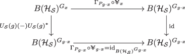
Proposition 3.4
The following statements hold.
-
1.
\(( \Gamma _{P_{x}} \circ \yen _{x} ) = \textrm{id}_{B(\mathcal {H}_{\mathcal {S}})^{G_x}}\)
-
2.
\(( \Gamma _{P_{g\cdot x}} \circ \yen _{x} )\) is equal to the isomorphism
$$B(\mathcal {H}_{\mathcal {S}})^{G_{x}} \rightarrow B(\mathcal {H}_{\mathcal {S}})^{G_{g \cdot x}} \; , \; A \mapsto U_{\mathcal {S}}(g) A U_{\mathcal {S}}(g)^* .$$ -
3.
The following diagram commutes:
-
4.
\(\Gamma _{\frac{1}{d} \mathbb {I}} \circ \yen _x\) and \(\Gamma _{P_{1}} \circ \yen _x\) are both equal to the surjective map
$$\begin{aligned} B(\mathcal {H}_{\mathcal {S}})^{G_x} \rightarrow B(\mathcal {H}_{\mathcal {S}})^{G} \; , \; A \mapsto \frac{1}{|G|} \sum _{g \in G} U_{\mathcal {S}}(g) A U_{\mathcal {S}}(g)^* . \end{aligned}$$(6)

Proof
-
1.
This is a special case of 2.
-
2.
Using the fact that the projections \(P_{x}, P_{y}\) are orthogonal for \(x \ne y\), we have that
$$\begin{aligned} (\Gamma _{P_{g\cdot x}} \circ \yen _{x}) (A)&= \sum _{kG_{x} \in G/G_{x}} \textrm{tr}( P_{g\cdot x} P_{k \cdot x} ) U_{\mathcal {S}}(k) A U_{\mathcal {S}}(k)^* \\&= \textrm{tr}( P_{g\cdot x}^{2} ) U_{\mathcal {S}}(g) A U_{\mathcal {S}}(g)^* \\&= U_{\mathcal {S}}(g) A U_{\mathcal {S}}(g)^* . \end{aligned}$$The map
$$B(\mathcal {H}_{\mathcal {S}})^{G_{x}} \rightarrow B(\mathcal {H}_{\mathcal {S}})^{g G_{x} g^{-1}} \; ,\; A \mapsto U_{\mathcal {S}}(g) A U_{\mathcal {S}}(g)^*$$is a C*-algebra isomorphism, and \(gG_{x}g^{-1} = G_{g \cdot x}\).
-
3.
Direct computation.
-
4.
For any invariant state \(\rho\), the equivariance of P means \(\text {tr}\left[ P_x \rho \right] =\text {tr}\left[ P_{g\cdot x}\rho \right]\) for all g and x, and hence the distribution \(y \mapsto p^P_{x}(y)\) is uniform and equal to \(\frac{1}{n}\) (recall that \(n = \textrm{dim}~L^2(X) = |G/G_x|\)). Therefore for any invariant \(\rho\),
$$\begin{aligned} (\Gamma _{\rho } \circ \yen _{x}) (A)&=\sum _{gG_{x} \in G/G_{x}} U_{\mathcal {S}}(g) A U_{\mathcal {S}}(g)^* \text {tr}\left[ \rho P_{g.x}\right] \\&= \frac{1}{n}\sum _{gG_{x} \in G/G_{x}} U_{\mathcal {S}}(g) A U_{\mathcal {S}}(g)^*\\&= \frac{1}{|G/H|}\frac{1}{|H|}\sum _{gG_{x} \in G/G_{x}} \sum _{h \in G_x} U_{\mathcal {S}}(gh) A U_{\mathcal {S}}(gh)^*,\\&= \frac{1}{|G|}\sum _{g \in G} U_{\mathcal {S}}(g) A U_{\mathcal {S}}(g)^*, \end{aligned}$$where in the final line we used that A is invariant under \(G_x\) and that \(|G|=n |G_x|\).
We interpret these findings as follows. Previous work (e.g. [15]) considered the setting \(X=G\) as a group, picking out the privileged point \(e \in G\), with the analogue of item 1. of Proposition 3.4 reading \((\Gamma _{P_e}\circ \yen ) = \textrm{id}_{B(\mathcal {H}_{\mathcal {S}})}\) (where \(\yen\) is defined as in (1) for finite G). This came with the interpretation that if the frame is localised at the identity (i.e., prepared in the vector state \(\delta _e\)), there is an exact agreement between the description of the system \(\mathcal {S}\) on its own, and with the inclusion of the appropriately prepared frame, thereby pointing to a condition on the frame that must be satisfied for the usual frameless/external description to apply. The deficiency of that work in contrast to the present formulation is twofold: first, it pertained only to the setting in which the underlying G space is (at least as a set) essentially equal to G, and second, it was contingent on an arbitrary choice of base point.
The present work remedies these issues: the \(\yen\) construction is now given as an X-parametrised family of maps, allowing for more general scenarios than \(X=G\) and restoring the egalitarian understanding of X as a collection of featureless points. This is reflected in item 1. of Propostion 3.4, in which the internal and external descriptions apply to each \(\yen _x(A)\), given a state localised at \(x \in X\). Moreover, by item 2., for any given \(x \in X\), the algebras defined through localisation at g.x are manifestly isomorphic and contain the same physical information—as can be seen explicitly from item 3. This demonstrates that simply reorienting the frame does not change the description in any essential way. We also observe that localisation at x still yields a \(G_x\)-invariant description, owing to the fact that \(\yen _x\) can only make sense on \(G_x\)-invariant operators. This is a direct analogue of a result in [10], where it is noted that in the presence of a non-trivial stabiliser for the frame, “the quantum frame can only resolve those properties of the remaining subsystems that are also invariant under its isotropy [stabiliser] group". In other words, even if \(\mathcal {S}\) has ostensibly \(G_x\) non-invariant properties (more properly understood as manifested with respect to a complete frame), these can never be observed by any frame with a \(G_x\) stabiliser. Item 4. shows that invariant reference states (noting that there always exists at least one pure and one mixed invariant state) gives rise to a finite version of the ‘G-twirl’, prevalent in the quantum information approach to QRFs [5]. This is used there to ‘remove’ any external frame dependence, where the frame is understood as localised but the actual value is not known, and the averaging captures the lack of knowledge of the exact orientation. Here, the interpretation is that the quantum reference state is completely indeterminate (with respect to G), and thus it is not surprising that the description of \(\mathcal {S}\) relative to an indeterminate state carries no dependence on G. In other words, only invariant states/observables can be used to describe \(\mathcal {S}\) and the G-sensitivity is completely washed out by the G-twirl operation.
3.3 Further Analysis
The canonical PVM P on X defines a rank-1 POVM on G by pulling back along the quotient map. This allows us to connect the perspective drawn up in this paper with that based on coherent states given in [10].
We begin by observing that fixing a base point \(x \in X\) determines a map
If \(H := G_{x}\), then under the isomorphism
the map \(\pi\) corresponds to the quotient map
The PVM \(P : X \rightarrow B(L^2(X))\) can be pulled back along \(\pi\) to define a map \(P \circ \pi : G \rightarrow B(L^2(X))\). Normalising this map then defines a POVM on G:
The positivity of each \(E_g\) is guaranteed by the positivity of \(\frac{1}{|H|}\); this prefactor is introduced to make sure \(E(X)= \mathbb {I}\):
Again, given a state \(\omega\) we call the probability distribution \(p^E_{\omega } = \text {tr}\left[ E_{\cdot }\omega \right]\) localised at \(g \in G\) if \(p^E_{\omega } = \delta _g\).
Proposition 3.5
The following are equivalent:
-
1.
X is a principal homogeneous space, i.e., \(G/H = G\)
-
2.
H is trivial.
-
3.
E is sharp (projection-valued).
-
4.
E satisfies the norm-1 property.
-
5.
For each \(g \in G\), there exists a state \(\omega\) on \(B(L^2(X))\) such that \(p^E_{\omega }\) is localised at g.
-
6.
For each \(g \in G\), there exists a pure state \(\omega\) on \(B(L^2(X))\) such that \(p^E_{\omega }\) is localised at g.
Proof
1. \(\Leftrightarrow\) 2. Standard.
2. \(\Leftrightarrow\) 3. H is trivial iff \(|H| = 1\) iff \(E_{g} = 1/|H| P_{gH}\) is a projection.
3. \(\Leftrightarrow\) 4. Any sharp observable satisfies the norm-1 property. Since \(E(g) = 1/|H|P_{gH}\), E(g) can satisfy the norm-1 property only if \(|H|=1\) in which case E is sharp. The rest follows from Prop. 2.2. \(\square\)
Remark 3.6
Some of the statements also follow from the observation that if H is non-trivial then \(|G| > \textrm{dim} \; L^2(X)\) and so there cannot exist a PVM from G to \(B(L^2(X))\).
Remark 3.7
Since each \(E_g\) is rank-1 and E is covariant, we can write \(E_g=(1/|H|)|g\rangle \langle g|\), the collection of which therefore make up a coherent state system, making contact with [10]. This will be discussed further in subsection 3.4.
We can now write the \(\yen\) map in terms of E; again we fix a base point \(x \in X\), set \(H:= G_{x}\), and identify X with G/H. Using the POVM E one can define a linear map
Proposition 3.8
For \(A \in B(\mathcal {H}_{\mathcal {S}})\) it holds that
In particular, the map \(\yen ^{E}\) factors as
where \(\textrm{av}_{H}\) is the average over H or H-twirl:
Proof
We have
as required. \(\square\)
From here we see that one is forced to average/twirl observables over H, which ‘washes out’ any H-dependence (precisely, and H-non-invariance in A). Under restriction \(\Gamma _{\omega }\), the above result shows clearly how statistics of non-H-invariant states/observables for \(\mathcal {S}\) can never arise; even if \(\omega\) is localised on the coset eH, the resulting observable is twirled over H. This is in line with the philosophy of [10] - that the frame enforces its symmetry on the system, but this conclusion has been arrived at by different means.
3.4 Coherent States
We would like to compare our setup with that of [10], in particular with the notions and results contained in pp10-12. The POVM E can be understood as corresponding to a system of coherent states. We use Dirac notation to make the comparison as clear as possible.
At the level of vectors, we have a map
where the notation \(\tilde{E}\) is chosen to agree with [10]. The corresponding map to projections is
where \(E_g=1/|H|P_{gH}\) as defined in subsec. 3.3. The set \(\{ |gH\rangle \; | \; g \in G \}\) is a homogeneous space with action
In particular,
and the stabiliser of the base point \(|eH\rangle\) is H.
Proposition 3.9
The following are equivalent:
-
1.
The reference frame X is principal.
-
2.
H is trivial.
-
3.
The POVM E is a PVM.
-
4.
The system of coherent states \(\tilde{E}\) is complete in the sense of [10] p.11, which by definition means that the stabiliser of each \(|gH\rangle\) is trivial.
-
5.
The system of coherent states \(\tilde{E}\) is ideal in the sense of [10], p.11, which by definition means that the vectors \(|gH\rangle\) are orthogonal to each other.
If any of the above conditions do not hold, then the system of coherent states \(\tilde{E}\) is incomplete in the sense of [10], p.11.
The resolution of the identity property, up to scaling, holds:
where the factor of |H| arises because \(E_{g} = \frac{1}{|H|} |gH \rangle \langle gH|\). This corresponds to [10], p.11 (5).
The POVM E can be recovered from \(\tilde{E}\) as in [10], p. 11 (6):
The normalisation |H| is equal to \(\textrm{Vol}(H)\) in [10], p.12 (12). The factorisation of \(\yen ^{E}\), Proposition 3.8 above, is related to the factorisation of the integral in [10] p.12 (12).
3.5 Example: Permutations
For \(n > 2\) the symmetric group \(S_{n}\) of permutations of the set \(X = \{x_1,\dots ,x_n\}\) provides an example of a homogeneous space which is not principal. For the action we write
for \(\sigma \in S_n\) and \(1 \le i \le n\). The stabiliser of each element of X is a symmetric group on \(n-1\) symbols. Choosing \(x_n\) for clarity, the stabiliser is naturally identified with the symmetric group \(S_{n-1} \subset S_{n}\), and there is an isomorphism of \(S_{n}\)-sets
As an \(S_n\) representation the Hilbert space \(L^2(X)\) decomposes as
where \(\textrm{Stand}\) is the standard \(n-1\) dimensional irreducible representation of \(S_{n}\), which is
In particular, \(P_{\varvec{1}}\) is unique \(S_n\)-invariant pure state on \(B(L^2(X))\).
Let \(\mathcal {H}\) be a fixed Hilbert space, \(\mathcal {H}_{\mathcal {S}}= \mathcal {H}^{\otimes n}\), and \(S_{n}\) act on \(\mathcal {H}_{\mathcal {S}}\) by permuting tensor factors. The corresponding action on \(B(\mathcal {H}^{\otimes n}) \cong B(\mathcal {H})^{\otimes n}\) is by permuting tensor factors.
The domain of \(\yen _{j}\) is the algebra
where \((jn) S_{n-1} (jn)\) is the stabiliser of \(x_{j}\), and \(S_{n-1}\) is the stabiliser of \(x_n\). In particular, the domain of \(\yen _{n}\) is the algebra
If
is an element of \(B(\mathcal {H}_{\mathcal {S}})^{S_{n-1}}\) then
For the maps \(\Gamma _{\omega }\) defined by localised states, each of the maps
is an isomorphism, where \(1 \le i,j \le n\). In particular, for \(j=n\), these maps are
This exemplifies the behaviour witnessed in the general setting: the restricted relativised observables can be perfectly recovered up to \(S_{n-1}\) invariance, but no better.
4 Concluding Remarks
We have given a construction of quantum reference frames suited to finite homogeneous spaces and analysed the situation in which the reference observable is given by the canonical covariant PVM, which, as we have seen, reduces to the coherent state set-up given in [10]. The case of an unsharp reference observable has not been analysed here, but it is clear that it gives something more general than a system of coherent states on G. It is not clear if other advantages are afforded from the homogeneous space point of view. On the one hand it appears more classical than the prescription of [10], since it appears to be predicated upon the existence of some underlying space X. On the other, X can be interpreted as the value space of some observable E, and as such is more operational. Future work, involving also the compact and locally compact settings, should shed further light on the relative merits of each approach.
References
Eddington, A.S.: Fundamental theory (CUP Archive) (1946)
Aharonov, Y., Susskind, L.: Phys. Rev. 155, 1428 (1967)
Wick, G.C., Wightman, A.S., Wigner, E.P.: Physical Review D 1, 3267 (1970)
Aharonov, Y., Kaufherr, T.: Phys. Rev. D 30, 368 (1984)
Bartlett, S.D., Rudolph, T., Spekkens, W.: Rev. Mod. Phys. 79, 555 (2007)
Castro-Ruiz, E., Oreshkov, O.: Relative subsystems and quantum reference frame transformations (2021). arXiv:2110.13199
Vanrietvelde, A., Höhn, P.A., Giacomini F.: Switching quantum reference frames in the N-body problem and the absence of global relational perspectives. Quantum. 7, 1088 (2023)
Vanrietvelde, A., Hoehn, P.A., Giacomini, F., Castro-Ruiz, E.: A change of perspective: switching quantum reference frames via a perspective-neutral framework. Quantum 4, 225 (2020)
Krumm, M., Höhn, P.A., Müller, M.P.: Quantum reference frame transformations as symmetries and the paradox of the third particle. Quantum 5, 530 (2021)
de la Hamette AC, Galley TD, Hoehn PA, Loveridge L, Mueller MP.: Perspective-neutral approach to quantum frame covariance for general symmetry groups (2021). arXiv:2110.13824
Giacomini, F., Castro-Ruiz, E., Brukner, Č.: Phys. Rev. Lett. 123, 090404 (2019)
de la Hamette, A.C., Galley, T.D.: Quantum reference frames for general symmetry groups. Quantum 4, 367 (2020)
Loveridge, L.: Quantum measurements in the presence of symmetry, Ph.D. thesis, University of York (2012)
Loveridge, L., Busch, P., Miyadera, T.: EPL (Europhysics Letters) 117, 40004 (2017)
Loveridge, L., Miyadera, T., Busch, P.: Found. Phys. 48, 135 (2018)
Miyadera, T., Loveridge, L.: In Journal of Physics: Conference Series, Vol. 1638 (IOP Publishing, 2020) p. 012008
Miyadera, T., Loveridge, L., Busch, P.: J. Phys. A: Math. Theor. 49, 185301 (2016)
Loveridge, L., Miyadera, T.: Found. Phys. 49, 549 (2019)
Loveridge, L.: In Journal of Physics: Conference Series, Vol. 1638 (IOP Publishing, 2020) p. 012009
Carette T, Głowacki J, Loveridge L.: Operational Quantum Reference Frame Transformations (2023). arXiv:2303.14002
Głowacki J.: Operational Quantum Frames: An operational approach to quantum reference frames (2023). arXiv:2304.07021
Heinonen, T., Lahti, P., Pellonpää, J.P., Pulmannova, S., Ylinen, K.: The norm-1-property of a quantum observable. J. Math. Phys. 44, 1998 (2003)
Busch, P., Grabowski, M., Lahti, P.J.: Operational quantum physics, Vol. 31 (Springer Science & Business Media, 1997)
Williams, DP.: Crossed Products of \(C^{*}\)-Algebras, 134 (American Mathematical Soc., 2007)
Serre, J.-P., et al.: Linear representations of finite groups, Vol. 42 (Springer, 1977)
DeWitt, B.S.: Quantum theory of gravity. I. The canonical theory. Physical Review. 160(5), 1113 (1967)
Rieffel, M.A.: Math. Scand. 47, 157 (1980)
Connes, A.: Noncommutative Geometry (Academic Press, 1994)
Waldron, J., Loveridge, L.D.: Skew Hecke Algebras (2023). arXiv:2311.09038
Acknowledgements
LL would like to thank the Theoretical Visiting Sciences Programme (TSVP) at the Okinawa Institute of Science and Technology for enabling his visit, and for the generous hospitality and excellent working conditions during his time there, during which part of this work was completed. JW would like to thank USN for their hospitality during his visit in early 2023. Thanks are also due to M. H. Mohammady for feedback on an early draft of this paper, to Stefan Ludescher for an extremely careful reading of the first, and to the audience of the seminar at IQOQI for some interesting and important questions which helped to sharpen our thinking on a number of issues.
Author information
Authors and Affiliations
Corresponding author
Additional information
Publisher's Note
Springer Nature remains neutral with regard to jurisdictional claims in published maps and institutional affiliations.
Rights and permissions
Open Access This article is licensed under a Creative Commons Attribution 4.0 International License, which permits use, sharing, adaptation, distribution and reproduction in any medium or format, as long as you give appropriate credit to the original author(s) and the source, provide a link to the Creative Commons licence, and indicate if changes were made. The images or other third party material in this article are included in the article's Creative Commons licence, unless indicated otherwise in a credit line to the material. If material is not included in the article's Creative Commons licence and your intended use is not permitted by statutory regulation or exceeds the permitted use, you will need to obtain permission directly from the copyright holder. To view a copy of this licence, visit http://creativecommons.org/licenses/by/4.0/.
About this article

Cite this article
Głowacki, J., Loveridge, L. & Waldron, J. Quantum Reference Frames on Finite Homogeneous Spaces. Int J Theor Phys 63, 137 (2024). https://doi.org/10.1007/s10773-024-05650-7
Received:
Accepted:
Published:
DOI: https://doi.org/10.1007/s10773-024-05650-7