
Abstract
We investigate whether a profit-maximizing insurer with the opportunity to modify the loss probability will engage in loss prevention or instead spend effort to increase the loss probability. First we study this question within a traditional expected utility framework; then we apply Kőszegi and Rabin’s (2006, 2007) loss aversion model to account for reference-dependence in consumer preferences. Largely independent of the adopted framework, we find that the profit-maximizing loss probability for many commonly used parameterizations is close to 1/2. So in cases where the initial loss probability is low, insurers will have an incentive to increase it. This qualifies appeals to grant insurers market power to incentivize them to engage in loss prevention.
1 Introduction
An insurer’s profits depend on how much consumers are willing to pay for protection against a potential loss in excess of the expected value of the policy, the risk premium. This risk premium in turn is a function of both the severity of the loss and the probability that a loss happens. It seems only natural for profit-maximizing insurers to influence either or both of these risk management parameters whenever possible. Despite this connection, and in sharp contrast to the extensive literature that deals with the insuree’s incentives to engage in self-protection and self-insurance,Footnote 1 attention for the loss-modification incentives by insurers has been very limited.
Two notable exceptions are the contributions by Schlesinger and Venezian (1986, 1990) who point out (1990, p. 84) that insurers often lobby Congress to implement policies aimed at loss prevention (e.g. keep drunk drivers off the road) or loss reduction (e.g. mandatory airbags and better bumpers on new automobiles). Within an expected-utility framework with risk-averse consumers, they formalize the decision problem of a risk-neutral monopolistic insurer who has the possibility to modify the status-quo loss probability \(p_0\). When any loss modification efforts are costless, the insurer has incentives to invest in loss prevention services prior to any insurance sales when the status-quo probability \(p_0\) exceeds the profit-maximizing probability \(p^*\). Because the insurer always sets the risk premium such that the consumer’s utility when buying insurance is marginally higher than the expected utility of being uninsured, and because the latter is decreasing in the loss probability, any reduction in loss probability will unambiguously increase consumer welfare.
On the other hand, in case the status quo loss probability \(p_0\) is lower than the profit-maximizing probability \(p^*\), the interest of the insurer to increase the loss probability unambiguously goes against the interest of consumers. To illustrate, consider the recent development of driverless cars. Automated vehicle technology is predicted to reduce both the number of cars on the road and the number of fatal crashes.Footnote 2 While clearly benefiting consumers, the market for car insurance is likely to suffer.Footnote 3 Indeed, insurance companies like e.g. the Cincinnati Financial Corporation (2015) have started warning in their SEC filings that self-driving cars pose a threat to their business: “Disruption of the insurance market caused by technology innovations such as driverless cars that could decrease consumer demand for insurance products” (p. 111). Insurance companies thus seem to have incentives to obstruct this development although direct evidence that they actually do so is absent.Footnote 4
In Schlesinger and Venezian’s work, this possibility receives relatively little attention, because it is “likely to meet with public resistance and possible regulatory restraint” (Schlesinger and Venezian 1990).Footnote 5 This view that society provides sufficient checks and balances to prevent insurers from taking actions against the interest of consumers may however prove too optimistic. Whereas insurers’ loss reduction activities are easy to monitor because companies are happy to advertise themFootnote 6, any omitted loss-prevention activities or efforts to increase the loss probability are likely to go unobserved. In this paper, we do not provide clear-cut empirical examples of monopolistic insurers using their market power to obstruct threats that threaten their product markets; our purpose is to show that this is not because it is not a theoretical possibility.Footnote 7
The final verdict on whether it is in the consumer’s interest to grant insurers market power in specific markets therefore depends on the relative importance of welfare gains of the increased bargaining power of insurers vis-à-vis providers and the welfare loss due to the modification of loss probabilities.
In this paper, we calculate for a number of settings the value of the profit-maximizing loss probability with the idea that the higher this value, the less likely it is that the initial loss probability is even higher and the less likely that consumers would be better off in an insurance market with less competition. First we consider the expected-utility framework. We repeat the analysis in Schlesinger and Venezian (1990) for an economy in which consumers are endowed with CARA preferences, which describes the case where consumers face absolute losses. Next we describe the situation where consumers have CRRA preferences, which describes situations where they have to choose whether or not to insure against a potential loss proportional to their wealth. In both cases, the optimal loss probabilities only come close to zero if consumers are highly risk averse (CARA) or are highly risk averse and face the risk of losing a large fraction of their initial wealth (CRRA).
In the second part of the paper, we use the more recent loss aversion theory to analyze the insurer’s problem of finding the optimal loss probability in case the consumers have reference-dependent preferences. We apply the reference-dependent utility model introduced by Kőszegi and Rabin (2006, 2007) to extend our analysis of the insurer’s loss prevention activities to situations where consumers have reference-dependent preferences. This approach is novel and complements other contributions that study the implications of the Kőszegi-Rabin framework on firm strategy and competition in non-insurance markets (Heidhues and Kőszegi 2008, 2014; Carbajal and Ely 2014). Models of loss aversion have also been applied in the field of insurance, but most of these contributions focus on the household’s decision-making problem rather than on the implications for the optimal strategy for insurance companies (Hu and Scott 2007; Sydnor 2010; Barseghyan et al. 2013).Footnote 8
Our main finding is that in most commonly used specifications, the loss probability that maximizes a monopolistic insurer’s profits is closer to 1/2 than to 0, independent of whether we adopt an expected-utility framework or take the perspective of loss-averse consumers. As a consequence, the instances where consumers are better off in a monopolistic than in a competitive insurance market seem to be fairly few. For this reason, our paper not only is an extension to the original work by Schlesinger and Venezian (1986, 1990), but also serves as a useful counterweight to other papers such as McKnight et al. (2012) that conclude that consumers may benefit from insurer market power.Footnote 9
2 Expected Utility Framework
This section deals with the optimal loss-size problem in the expected utility framework. We assume that consumers are risk-averse with a twice differentiable utility function of final wealth W with \(U^{'}(\cdot )>0\) and \(U^{''}(\cdot )<0\). The monopolistic insurer is risk-neutral. We follow Schlesinger and Venezian (1986, 1990) and consider only full coverage insurance and assume complete information for both parties. This allows us to abstract away from issues of deductibles, moral hazard and adverse selection. Whereas they consider both the case where loss prevention activities can be bundled with an insurance policy and the case where the insurers can alter the loss probability only before selling insurance, we focus on the latter case.
Consider a monopolistic insurance market where consumers have a wealth W and face a wealth prospect \(W-x\) where W is the present value of lifetime income and x a binary random variable that takes the value L with probability p and 0 otherwise. A key element of our model is that the insurer has the ability to costlessly change p. Consumer i will buy insurance if and only if:
with R denoting the premium.Footnote 10 The insurer’s decision problem is to set the premium R and the loss probability p at values that maximize the insurer’s expected profits:
where N denotes population size and \(I[\cdot ]\) is an indicator function. The first term denotes the expected profit per insuree and the summation gives the aggregate demand for insurance. Schlesinger and Venezian (1986, 1990) focus on the case where consumers have identical risk preferences. In this case, demand for insurance is either N or 0 for any (R, p)-combination. For any given p, a profit-maximizing insurer will set the price of the policy R(p) such that \(U(W-R)=(1-p)U(W)+pU(W-L)\). That is
with \({ CE }(p)\) denoting the certainty equivalent to the wealth prospect \(W-x\). This price equals the actuarial value of the policy, pL (i.e. the expected loss), plus a fixed fee equal to the consumer’s risk premium.Footnote 11 For this general setup, Schlesinger and Venezian (1986) show that for any loss size \(L<W\), there exists a unique loss probability \(p^*\) that maximizes the insurer’s expected profit.Footnote 12 This situation is illustrated in Fig. 1. The monopolistic insurer has incentives to invest in loss prevention activities whenever \(p^*\) is smaller than the status-quo probability \(p_0\) in the market. In a perfectly competitive market, insurers lack such an incentive, because any increase in margin due to these activities will be immediately competed away. Whether consumers are better off in a monopolistic or a competitive market thus depends on whether any reduction in loss probability compensates for the policy being priced above its actuarial value in the monopoly market.

The expected profit maximizing loss probability \(p^*\)
2.1 Absolute Risks
Schlesinger and Venezian (1990) present a quantitative analysis of their model. Their setting can be thought of as one where consumers have to choose between a lottery \(\ell = p \circ -L \oplus (1-p) \circ 0\) or avoiding the lottery by paying R(p). That is, consumers go uninsured against the risk to lose an absolute sum L with probability p or they buy insurance. Schlesinger and Venezian assume a representative consumer with preferences that exhibit constant absolute risk aversion (CARA):
with \(\theta >0\) the level of risk aversion. CARA preferences makes the decision to insure independent of a consumer’s initial wealth level W.
For convenience, we repeat their main results. For a given loss size L, the loss probability that maximizes the insurer’s profits equals
Whether consumers are better off in an imperfectly or perfectly competitive market not only depends on the sign of the difference between the optimal and status-quo loss-probability (\(p^*\) and \(p_0\)) but also on the magnitude of the risk premium an insurer is able to charge when he has market power. Schlesinger and Venezian (1990) show that when the status-quo loss-probability \(p_0\) exceeds (is lower than) a critical loss probability \(p^c\), consumers are better (worse) off in terms of expected utility in a market with a loss probability \(p^*\) and a monopolistically priced policy than in a competitive market where insurance is sold at the actuarial value of the policy (that is, at the expected loss \(p_0L\), with a zero risk premium).
In the case of CARA preferences, this critical probability \(p^c\) equals
Note that \(p^cL=R(p^*)\). The term on the left hand side is the actuarially fair price consumers pay for coverage in a competitive market with loss probability \(p^c\), the right hand side the monopolistically priced policy with loss probability \(p^*\). Figure 2 depicts the optimal and critical loss probabilities for different loss sizes L. The left panel shows that the optimal probability is decreasing in the potential loss L consumers face. One can easily check the following result for the limiting cases of zero and infinite potential loss.Footnote 13

Plots of \(p^*(\theta )\) (left panel) and \(p^c(\theta )\) (right panel) under different calibrations of \(L=20, 40, 60, 80\) and 100 for \(\theta \in [0.01,0.99]\)
Result 1
Proof
All proofs are in the “Appendix”. \(\square \)
So, independent of the consumers’ level of risk aversion, the insurer has an interest in pushing down the status-quo loss probability as long as the loss L is sufficiently large; think of, for example, hospital expenses. For small losses, the insurer has an incentive to inflate the status-quo loss probability to the detriment of consumers unless one believes that the status-quo loss probability exceeds 0.5. Although hard evidence is absent, we do observe that insurance against small losses is often offered at a high price compared to the coverage. This implies that anyone who buys such policies is either extremely risk averse or perceives the loss as highly likely to happen to him or her.Footnote 14
The left panel of Fig. 2 shows that for given L, the optimal loss probability is decreasing in \(\theta \). This is because in selecting the loss probability, the insurer has to trade-off the negative effect of decreasing p on consumers’ willingness to pay (insuring against a loss is more valuable the higher the expected loss) against the positive impact a lower loss probability has on the fraction of clients suffering an actual loss (which reduces the insurer’s cost). For CARA utility and a given loss L, when society becomes more risk-averse the second effect dominates, such that the insurer lowers p when people become more risk-averse.
The right panel of Fig. 2 shows the critical loss probabilities for different loss sizes L. Note that for all values of L and \(\theta \), the status-quo probability has to exceed 0.5 for consumers to be better off in a monopoly market. In most cases it has to be higher than 0.7. For example, for \(\theta =0.3\) and \(L=40\), \(p^c\approx 0.79\) and \(p^*\approx 0.08\). Why are consumers not better off in a monopoly market despite the impressive reduction in loss probability? The reason is that the monopolistic insurer sets the price of the policy equal to the price that would be obtained under competition with the higher loss probability: \(R(0.08)= p^cL\approx 31.7\). Figure 3 illustrates this point by showing the ratio between the actual price of the policy \(R(p^*)\) and its actuarial value \(p^*L\). For \(L=5\), the risk premium seems reasonable, but as L increases, consumers are willing to pay a premium dozens of times the actuarial value, which implies absurdly high degree of risk aversion. This result is a direct consequence of the observation first made by Rabin (2000) and Rabin and Thaler (2001) that under CARA utility, the refusal of small bets implies absurd levels of risk aversion for large bets. In sum, when consumers are endowed with CARA preferences, the instances where they are better off in a monopolistic than a competitive insurance market seem to be fairly few.

Plot of the \(R(p^*)/(p^*L)\) ratio for the loss sizes \(L=20, 40, 60, 80, 95\) and 100 and initial wealth \(W=100\)
2.2 Proportional Risks
We next extend the analysis to the case where consumer preferences are characterized by constant relative risk aversion (CRRA). CRRA models are more common than CARA in the recent literature of insurance markets.Footnote 15 CRRA utility is given by
Since offering insurance is only profitable if there are risk-averse individuals, we limit attention to the case \(\theta >0\), ruling out situations where \(\theta =0\) (risk-neutrality) or \(\theta <0\) (risk-seeking).
After inserting (7) into the profit function (2) and taking the derivative with respect to p, we obtain the following general expression for the profit-maximizing loss probability as a function of the risk aversion parameter \(\theta \):Footnote 16
In the remainder of this section, we focus on the situation in which consumers face a loss proportional to their initial or discounted lifetime wealth, \(L=\delta W\). In other words, they face a lottery of the form \(\ell = p \circ -\delta W \oplus (1-p) \circ 0\). This seems an appropriate description for decisions concerning e.g. home insurance. With potential losses proportional to wealth, the optimal probability becomes wealth independent and Eq. (8) reduces to:
We have the following result:
Result 2
-
1.
\(\lim _{\theta \rightarrow 0} p^*(\theta )\Big |_{\delta =1}=1-e^{-1}\),
-
2.
\(p^*(1/2)=1/2\),
-
3.
\(\lim _{\delta \rightarrow 1} p^*(\theta )=1-(1-\theta )^{\frac{1-\theta }{\theta }}\),
-
4.
\(\lim _{\delta \rightarrow 0}p^*(\theta )=1/2\).
It is most insightful to discuss the implications of these properties together with Fig. 4 that shows the development of the optimal and critical loss probabilities for different values of \(\theta \) and \(\delta \).Footnote 17 As for CARA utility, we observe that \(p^*\) is decreasing with the level of risk-aversion among the population. The right panel of Fig. 4 shows that for all sizes of the potential loss and all levels of risk aversion, the status-quo probability has to exceed 0.5 for consumers to be better off in a monopoly market. Again, the instances where consumers are better off in a monopolistic insurance market seem few.
The left panel of Fig. 4 and Result 2 show that for values of the risk aversion parameter \(\theta \le 1/2\), \(p^*(\theta )\ge 1/2\), \(\forall \delta \). That is, a monopolistic insurer will not have any incentive whatsoever to push loss probabilities below 0.5 if consumers are only mildly risk averse. Moreover, according to property 4, the optimal loss probability is 0.5 for any level of risk aversion in the limiting case \(\delta \downarrow 0\). The figure shows that only in case of \(\delta \ge 0.95\) and high levels of risk aversion, the optimal loss probability drops to values importantly lower than 0.5. The reason is that in this case, a lowering of the loss probability only has a very limited impact on the price the insurer can charge while significantly reducing the expected cost. Wakker (2008) mentions that when large amounts of money are at stake, utility functions with \(\theta >1\) tend to best fit empirical data, implying that high-\(\delta \)/high-\(\theta \) combinations may not be that rare in practice, see also Hartley et al. (2014).
The right panel of Fig. 4 shows that, as in the CARA case, for any level of risk aversion and loss size, the status-quo probability has to exceed 0.5 for consumers to be better off in a monopoly market. The instances that give the insurer the strongest incentives to reduce the loss probability are exactly those for which the status-quo probability has to be very high in order for consumers to benefit from being in a monopolistic instead of a competitive market. So also for CRRA utility, we conclude that consumers are better off in a monopolistic insurance market only when the potential loss is close to one’s initial wealth and consumers have a high index of relative risk aversion.
2.2.1 Heterogeneous Risk Attitudes
So far, we have assumed representative consumers. Insurers however operate in markets where consumers differ in their risk attitudes and for this reason, we now lift the assumption to see how this will affect our results.Footnote 18 Since there is no closed form solution for \(p^*(\theta )\) in this case, we revert to simulation and present numerical results.
In line with Holt and Holt and Laury (2002), who estimate the coefficient of risk aversion for most subjects in a laboratory experiment to be in the 0.3–0.5 range, we draw individual risk preferences \(\theta _i\) from the distribution N(0.4, 0.1). To find the distribution of profit maximizing \((R(p^*), p^*)\)-combinations for a given proportional loss \(\delta \), we follow a three-step procedure: First we generate a total of \(N=1000\) consumers \((\theta _1, \theta _2, \ldots , \theta _{1000})\), with \(\theta _j\) independent draws from N(0.4, 0.1). Each consumer has initial wealth fixed at \(W=100\). Second we determine for each given loss probability p the optimal premium by calculating the quantity sold and profits obtained for each possible value of the premium \(R\in [pL:0.01:W]\); we then repeat this step for each probability \(p\in \mathcal {P}=\{0, 0.01,\ldots , 1.00\}\) and select the probability \(p^*\) for which \(\pi (p^*,R(p^*))\ge \pi (p',R(p'))\), \(\forall {}p'\in \mathcal {P}\). We repeat these three steps 1, 000 times in order to arrive at distributions of the optimal \(p^*\) and other market characteristics such as the percentage of consumers that takes out insurance and consumer welfare.
Table 1 gives the simulation results for different values of \(\delta \). The table shows that, similar to the homogeneous CRRA case with \(\theta <0.5\), the optimal loss probability is increasing in \(\delta \) but close to one half for all values of \(\delta \) considered. The equilibrium fraction of consumers insured is very similar for different values of \(\delta \). Figure 5 shows for \(\delta =0.2\) the simulated distributions of the optimal loss probability \(p^*\), the insurer’s profits, the premium \(R(p^*)\) set and the number of consumers that decides to buy insurance.

Normal Kernel density estimations and scatter plots for the simulation results (\(\delta =0.2\)). a \(p^*\). b \(\pi (p^*)\). c \(R(p^*)\). d Quantity
3 Reference-Dependent Utility
In the expected-utility model, recent changes in wealth do not affect the utility one derives from one’s current wealth. That is, a wealth level of $2 million gives you the same utility independent of whether you gained $1 million or lost $3 million compared to yesterday. This limited framework is unable to explain risk aversion over relatively small stakes because anything but virtually risk neutrality over small stakes implies absurd risk aversion over larger stakes (Rabin 2000). Samuelson (2005, p. 90) notes that although this is the common way expected utility appears in theoretical models, there are no fundamental objections to defining utility over initial wealth and changes in wealth. Kőszegi and Rabin (2006, 2007) develop such a model of reference-dependent utility in which the utility derived from a riskless wealth outcome consists of two components: an intrinsic “consumption utility” which is a function of the wealth outcome only, plus a reference-dependent gain-loss utility. Subsequent studies have applied this model to topics as disparate as cross-country differences in trust levels (Bohnet et al. 2010), a monopolistic firm’s pricing strategies when consumers have reference-dependent preferences (Heidhues and Kőszegi 2014; Carbajal and Ely 2014), price variation and competition intensity (Heidhues and Kőszegi 2008) and dynamic models of consumption plans (Kőszegi and Rabin 2009). This section analyzes the behavior of a profit-maximizing insurer who can influence loss probabilities in the reference-dependent utility framework. Our objective is to see whether the main finding of the previous section—the profit-maximizing loss probability is around 0.5 for commonly observed levels of risk aversion—is upheld in the Kőszegi and Rabin (2007) model.Footnote 19
The key element of Kőszegi and Rabin (2007) is that a person’s utility not only depends on her riskless wealth outcome \(w\in \mathbb {R}\), but also on a riskless reference level of wealth \(r\in \mathbb {R}\).Footnote 20 A representative consumer’s total utility is given by
with the term m(w) the intrinsic consumption utility and the term \(\mu (m(w)-m(r))\) the reference-dependent gain-loss utility. The model assumes that the reference point r relative to which a consumer evaluates an outcome is stochastic because a consumer may be uncertain about outcomes. When w is drawn according to the probability measure \(F(\cdot )\), utility is given by
The model makes the simplifying assumption that preferences are linear in probabilities: For a given reference point, the stochastic wealth outcome is evaluated according to its expected reference-dependent utility. This in contrast to prospect theory (Kahneman and Tversky 1979; Barberis 2013) that allows decision weights to be a non-linear function of the objective probabilities in order to accommodate the commonly observed phenomenon that people tend to overweigh small probabilities and underweigh large probabilities.Footnote 21
As in the previous section, consumers have to decide whether they wish to face the risk of losing L of their initial wealth W with probability p or to buy insurance against this risk by paying a premium R. To close the model, one needs to determine the appropriate reference point. Although there is little empirical evidence on the determinants of reference points, Kőszegi and Rabin (2006, 2007) make the case for a rational expectations assumption: A person’s reference point has to be consistent with the beliefs about the outcome this person held in the recent past. For example, an employee who had been expecting a salary of $100,000 and should assess a salary of $90,000 not as a gain but as a loss.Footnote 22
Kőszegi and Rabin (2007) distinguish between unanticipated and anticipated risks. Given our context, the case where agents anticipate the exposure to risk seem most appropriate. In these situations, the agent correctly predicts the choice set she faces. Within this class, Kőszegi and Rabin (2007) distinguish between UPE/PPE risk attitudes and CPE risk attitudes.
In the unacclimating personal equilibrium (UPE), the time between the decision (take insurance or not) and the outcome (a loss occurs or not) is sufficiently short that the agent does not adapt her expectations. That is, she will evaluate the gain-loss utility of the outcome relative to the expected outcome without coverage, and the agent knows she will evaluate outcomes this way (the rational expectations assumption). Kőszegi and Rabin (2007) mention insurance choice for short-term rentals such as cars and skis as examples.
Kőszegi and Rabin (2007) give an example for \(L=100\), \(p=0.5\) and \(R=55\). In deciding whether or not to take insurance, the agent will infer that a) taking insurance by paying 55 will induce either feeling of losing 55 with probability \(1-p=0.5\) (in case no loss occurs) or a feeling of gaining 45 (in case a loss does occur); b) not taking insurance will either lead to a mixed feeling of status quo and gaining 100 (in case no loss occurs) or a mixed feeling of status quo and loosing 100 (in case a loss does occur).
In the choice-acclimating personal equilibrium (CPE), it is assumed that the time between the moment of deciding and the moment of the outcome is sufficiently long to adapt expectations. That is, if the agent decides not to take insurance, this choice will determine her reference point at the time the relevant wealth outcome occurs and the possibility that she could have taken insurance does not enter the gain-loss calculation.Footnote 23 If she decides to take insurance, this will determine her reference point and the possibility that she could have chosen not to insure does not enter the gain-loss calculation. This situation adequately describes choice for travel and flight insurance.
To return to the numerical example, the agent will rightly infer that (a) taking insurance by paying 55 will not lead to any gain-loss utility because at the moment of the outcome, the risk that was once there will be forgotten; (b) not taking insurance will, just as in the UPE situation either lead to a mixed feeling of status quo and gaining 100 (in case no loss occurs) or a mixed feeling of status quo and loosing 100 (in case a loss does happen).
So, compared to UPE, taking insurance will be more attractive in a CPE context because it is never felt as a loss. The implication of the insurance being relatively more attractive is that agents are more risk averse when they anticipate a risk and the possibility to buy insurance coverage. We now continue with calculating the optimal loss probabilities under UPE and CPE.
3.1 Optimal Loss Probability Under UPE Risk Attitudes
In the remainder of this section, we assume that the consumption utility is linear, \(m(w)=w\). This is a reasonable assumption for modest scale risks. If being insured is the reference point, the expected utility of a consumer with initial endowment W who decides to buy insurance by paying a premium R equals
where the last equality follows because (i) in case of being covered, there is no uncertainty in the final wealth received, \(f(W-R)=1\); (ii) if being insured is the reference point, the probability measure of the reference point has mass 1 at \(W-R\) as well. There is no feeling of loss or gaining in this case.
If being insured is the reference point but the consumer decides not to buy insurance, her expected utility is:
where the last equality follows from \(f'(W-L)=1-f'(W)=p\) and \(f(W-R)=1\): without insurance, the wealth outcome is \(W-L\) with probability p and \((W-L)\) otherwise; the reference point is \((W-R)\) with probability 1. Applying Kőszegi and Rabin’s (2007) definition, the decision to buy insurance is an UPE if \(U(F|F)\ge {}U(F'|F)\).
Assuming that consumers will buy insurance whenever the expected utility of being insured is at least as large as the expected utility of not being insured, a risk-neutral monopolistic insurer who aims to maximize expected profits will set the loss probability p such that \(R-pL\) is maximal, conditional on \(U(F|F)\ge U(F'|F)\). In order to find an explicit solution for \(p^*\), we use the same parametrization of the reference-dependent gain-loss utility \(\mu (\cdot )\) as Kőszegi and Rabin (2006, 2007): \(\mu (x)=\eta {}x\) for \(x>0\), and \(\mu (x)=\eta {\uplambda }{}x\) for \(x\le {}0\), with \(\eta >0\) the relative weight that consumers attach to gain-loss utility, and \({\uplambda }>1\) the coefficient of loss aversion. Given this specification:
We arrive at the following result (a detailed derivation is provided in Appendix 1):
Result 3
In an economy where consumers’ attitude towards risk is characterized by UPE, the loss probability \(p^*\) that maximizes the expected-profits of a monopolistic insurer equals
and the corresponding price of the insurance is
One easily sees that \({\uplambda }>1\) guarantees positive expected profits per insuree, \(R(p^*)-p^*L\). Note that, different from the expected-utility framework, the loss size L does not appear as an argument. A number of other properties of \(p^*\) are stated in the following corollary.
Corollary 1
The loss probability \(p^*\) as given in Eq. (14) has the following properties
-
1.
\(\frac{\partial p^*}{\partial \eta }<0\).
-
2.
\(\lim _{\eta \downarrow 0} p^*=1/2.\)
-
3.
\(\lim _{\eta \rightarrow \infty } p^*=\frac{\sqrt{{\uplambda }}-1}{{\uplambda }-1}.\)
The first property says that the optimal loss probability is decreasing with the relative importance of the gain-loss utility. Taken together, the properties inform us that for a given \({\uplambda }\), \(p^*\in \left[ \frac{\sqrt{{\uplambda }}-1}{{\uplambda }-1}, \frac{1}{2}\right] \). Empirical studies typically find estimates of the loss aversion parameter \({\uplambda }\) of around 2.25 (Kahneman et al. 1990; Tversky and Kahneman 1992; Gill and Prowse 2012). Such an estimate implies a lower bound for the optimal loss probability of 0.4. So, again, we find values of \(p^*\) much closer to 1/2 than to 0.
Another possible UPE is the situation where no insurance is the reference point and the decision not to buy insurance gives the consumer a higher expected utility than buying insurance, that is: \(U(F'|F')\ge U(F|F')\). Kőszegi and Rabin (2006) propose that in cases with multiple equilibria, an individual will choose her “favorite” equilibrium, the one that gives the highest ex ante expected utility if followed through. This leads to the concept of ‘preferred personal equilibrium’ (PPE) as an equilibrium selection mechanism: the PPE is the most preferred UPE. In our case, deciding to buy insurance is a PPE if \(U(F|F)\ge U(F'|F')\). The assumption of profit-maximization by the insurer rules out that \(U(F|F)<U(F'|F')\) because in that case, the insurer’s profits would be zero and because—as we will show in the next section—there is always a feasible loss probability p such that his expected profits are non-negative and \(U(F|F)\ge U(F'|F')\) holds.
3.2 Optimal Loss Probability Under CPE Risk Attitudes
One of the implications of Kőszegi and Rabin’s model is that buying insurance is more attractive when consumers have CPE instead of UPE risk attitudes. This implies that insurers are better off when consumers can buy insurance well ahead of time. We explore this possibility in this section. The expected utility of taking insurance U(F|F) does not change and equals (12). The expected utility of the decision not to buy insurance, given that the reference point is also “no insurance”, equals
Without insurance, the wealth outcome is W with probability \(f'(W)=1-p\) and \((W-L)\) with probability \(f'(W-L)=p\). The reference point is ‘no insurance’ in which case the outcome is also W with probability \((1-p)\) and \((W-L)\) otherwise.
Buying insurance is a CPE if \(U(F|F)\ge {U(F'|F')}\) for all \(F'\). The monopolistic insurer sets p such that the expected profits are maximized under the condition that \(U(F|F)\ge {U(F'|F')}\). Equating \(U(F'|F')\) in Eq. (16) to U(F|F) in Eq. (12) shows that in equilibrium, the expected profit margin of the insurer equals
In prospect theory, the gain-loss utility is assumed concave in the region of gains but convex in the region of losses. This property of diminishing sensitivity implies that \(\mu (+L)+\mu (-L)<0\) such that expected profits are maximized when \(p^*=1/2\). We state this result formally:
Result 4
In an economy where consumers’ attitude towards risk is characterized by CPE, the loss probability \(p^*\) that maximizes the expected-profits of a monopolistic insurer equals 1 / 2.
Note that this result is reached without assuming any specific parametrization for the gain-loss utility function. Figure 6 provides some intuition for this result. In the figure, the loss-averse utility function \(U(F'|F')\) of Eq. (16) is convex with respect to p.Footnote 24 When \(p=p^*\), an individual’s utility equals \(U(p^*)\) if she is loss-averse and (\(W-p^*L\)) if risk-neutral. Since we assume linear consumption utility, the certainty equivalent equals \({ CE }(p)=U({ CE }(p))\). Thus the expected profit equals the distance marked by the vertical dotted line. The optimal loss probability \(p^*\) maximizes the distance between \(U(F'|F')\) and the expected wealth line \(W-pL\), which is the point p where \(U'(p)\) equals the slope of the expected wealth line, which is \(-L\). This maximal distance is attained when \(p^*=1/2\) because \(U'(F'|F')=-L+(1-2p)[\mu (L)+\mu (-L)]\).

CPE risk attitudes and the risk premium with linear consumption utility
For the specific parametrization \(\mu (x)=\eta x\) for \(x>0\) and \(\mu (x)={\uplambda }\eta x\) for \(x\le 0\), the profit maximizing premium and profits are equal to
and
The premium \(R^*\) is increasing in the weight of the gain-loss utility in the utility function and in \({\uplambda }\). This means that, in line with intuition, the more an individual weighs losses relative to gains, the higher the profit an insurer can attain.
Our result that \(p^*=1/2\) when consumers have CPE risk attitudes is qualitatively similar to the results for UPE risk attitudes and for the expected utility model. Compared to the UPE case individuals are more inclined to take out insurance because they are more risk-averse when they can commit to the choice ahead of time. The model we discuss in this section only considers a representative agent economy. Note however that for CPE risk attitudes, heterogeneity in either \(\eta \) or \({\uplambda }\) does not change our result because \(p^*\) does not depend on these values.
3.3 Numerical Example
We conclude this section with a numerical example. Assume that the consumer with a gain-loss coefficient \({\uplambda }=2.25\) has to decide whether or not to insure against a risk that leads to a loss \(L=10\) with probability \(p^*\). Table 2 compares for different values of \(\eta \) the expected-profit maximizing loss probability \(p^*\) and premium for the case where consumers have UPE risk attitudes with the case where they have CPE risk attitudes. The table also gives the expected profits per insuree and the ratio of the premium charged (\(R(p^*)\)) and the actuarial value of the policy (\(p^*L\)).
In line with the analytical results, the numerical results show that as the gain-loss utility receives higher weight, the optimal loss probability decreases in the UPE case. The premium and expected profits are increasing in \(\eta \), both for UPE as for CPE. Table 2 confirms that the monopolistic insurer is able to attain higher expected profits when consumers have CPE preferences. This difference is very sizable: whereas in the UPE case the premium rises to about 1.5 times the actuarial value, it rises to 63 times the actuarial value in the CPE case. This is reminiscent of our earlier findings for the expected utility model were consumers were endowed with CARA preferences (see Fig. 3).
4 Summary and Conclusions
This paper follows up on the original contributions by Schlesinger and Venezian (1986, 1990) who first investigated the incentives for loss-modification by profit-maximizing insurers. They concluded that granting insurers market power might benefit consumers because this might trigger them to exert efforts to bring down the ex ante loss or the probability with which such a loss occurs.
In this paper, we calculate for a number of settings the value of the profit-maximizing loss probability. First we consider the expected-utility framework where we repeat the analysis in Schlesinger and Venezian (1990) for an economy in which consumers are endowed with CARA preferences and add the situation where consumers have CRRA preferences. In both cases, the optimal loss probabilities only come close to zero if consumers are highly risk averse (CARA) or are highly risk averse and face the risk of losing a large fraction of their initial wealth (CRRA).
In the second part of the paper, we use the more recent loss aversion theory to analyze the insurer’s problem of finding the optimal loss probability in case the consumers have reference-dependent preferences. We use the reference-dependent utility model developed by Kőszegi and Rabin’s (2006, 2007) to show that under the assumption of linear consumption utility, the optimal loss probability is 0.5 when consumers have CPE risk attitudes and between 0.4 and 0.5 when consumers have UPE risk attitudes and a gain-loss coefficient of 2.25, a value often found in empirical studies.
Our overall conclusion therefore is that in most commonly used specifications, the loss probability that maximizes a monopolistic insurer’s profits is closer to 1/2 than to 0, independent of whether we adopt an expected-utility framework or take a more behaviorial perspective. This value is higher than many of loss probabilities consumers face for everyday risks. This implies that in evaluating the welfare effects of insurer market power, policy makers should not limit attention to the possible gains from increased insurer engagement in loss prevention activities but they should also eye the possibility that the modification of loss probabilities moves in a direction detrimental to consumer welfare.
Notes
The RAND Corporation expresses this view in a recent study: “If these technologies reduce crashes sufficiently, it is possible that the very need for specialized automobile insurance may disappear entirely.” (Anderson et al. 2014, p. 115).
The Association of California Insurance Companies (ACIC) has advocated for changes “clarifying the autonomous vehicle’s manufacturer retain all liability for damage, losses or injuries caused by the operation of these vehicles as required by the enabling law (SB 1298)”. As the RAND authors note, such shifts in liability from driver to manufacturer possibly lead to a “lower adoption of this technology than would be socially optimal.” (Anderson et al. 2014, p. 118).
Schlesinger and Venezian (1986, p. 232) use a similar argument to limit the subsequent analysis (“for the sake of concreteness”) to the case \(p^*<p_0\).
For example, insurers provide a variety of loss preventions services to reduce the probability of car theft (http://www.aig.com/motor-fleet-loss-control_2538_367524.html) or the number of hospital visits by offering free gym memberships to increase citizen’s enthusiasm for physical exercises (http://articles.washingtonpost.com/2012-01-12/politics/35439261_1_gym-membership-medicare-advantage-health-insurance) or by offering free medical check-ups.
Even when the insurer has no means to raise the actual loss probability, it may be in his interest to try to increase the subjective loss probability as perceived by consumers because a successful attempt will increase his profits. Arguably, policy makers may counteract this by investing in (costly) programs to increase consumer’s probability numeracy.
Barberis (2013) contains a summary of this literature.
In their empirical study, McKnight et al. (2012) find that insurers pay less than the uninsured for certain health services and conclude from this that “market power for insurers can offset provider market power (p. 10)”.
We assume that when consumers are indifferent between taking insurance or not, they choose to insure.
For concave utility functions it follows from Jensen’s inequality that \(U(W-pL)\ge {}pU(W-L)+(1-p)U(W)\) which is equivalent to \(W-pL\ge {}U^{-1}[pU(W-L)+(1-p)U(W)]\) because of \(U'>0\). Thus \(R(p)=W-U^{-1}[pU(W-L)+(1-p)U(W)]\ge pL\). That is, for any p, R(p) is such that the insurer’s expected profits \(R(p)-pL\) are non-negative.
It also follows from the strict concavity of the utility function that \(\pi ''(p)<0\). That is, that there are no local maxima besides \(p^*\), cf. Schlesinger and Venezian (1990, p. 85 equation (5)).
Schlesinger and Venezian (1990, p. 88) already mention this result in passing without giving a formal proof.
For example, a two-year insurance that covers breakage of prescription glasses with a value up to £100 costs £9 (http://www.visionexpress.com/glasses/buyers-guide/breakage-protection/).
Insert (7) and (3) into profit function (2), taking first-order condition and we arrive at
$$\begin{aligned} \pi (p)=&R(p)-pL=W-{ CE }(p)-pL=W-U^{-1}[U(W)-p(U(W)-U(W-L))]-pL\\ =&W-(W^{1-\theta }-p(W^{1-\theta }-(W-L)^{1-\theta }))^{\frac{1}{1-\theta }}-pL;\\ \pi '(p)=&-\frac{1}{1-\theta }(W^{1-\theta }-p(W^{1-\theta }-(W-L)^{1-\theta }))^{\frac{1}{1-\theta }-1}(-W^{1-\theta }+(W-L)^{1-\theta })-L=0\\ \Rightarrow&{}(W^{1-\theta }-p(W^{1-\theta }-(W-L)^{1-\theta }))^{\frac{1}{1-\theta }-1}=\frac{L(1-\theta )}{W^{1-\theta }-(W-L)^{1-\theta }}\\ \Rightarrow&{}p^*=\frac{W^{1-\theta }-\left[ \frac{L(1-\theta )}{W^{1-\theta }-(W-L)^{1-\theta }}\right] ^{\frac{1-\theta }{\theta }}}{W^{1-\theta }-(W-L)^{1-\theta }}. \end{aligned}$$We would like to point out that, other than ease of exposition, there no reason to neglect values of \(\theta > 1\) (see Wakker 2008, p. 1330-1332).
Fig. 4 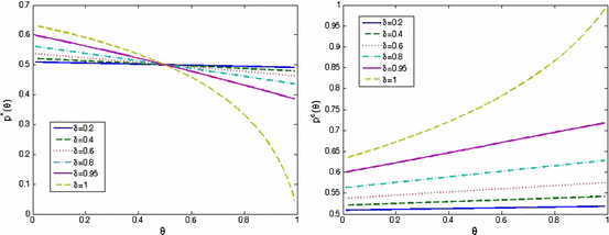
Plots of \(p^*(\theta )\) (left panel) and \(p^c(\theta )\) (right panel) for \(\delta =0.2, 0.4, 0.6, 0.8, 0.95\) and 1
We assume that the insurer only knows the distribution \(f(\theta )\) of \(\theta \) such that he cannot engage in first-degree price discrimination.
This simplification may lead us to underestimate the demand for insurance for low-probability losses.
Their main reasons for assuming rational expectations are that it maintains modeling discipline and that there is empirical evidence indicating that reference points are influenced by expectations (Post et al. 2008).
Phrased a bit differently, the CPE is defined as the decision that maximizes expected utility given that it determines both the reference lottery and the outcome lottery (Kőszegi and Rabin 2007).
Because we assume linear consumption utility, plotting the wealth level at the horizontal axis, as in Schlesinger and Venezian (1986, Figure 1) leads to linear utility curves. For this reason, we use the decision variable p as the variable at the horizontal axis.
To show that \(U'(F'|F')\) is convex, take the first order and second order derivatives w.r.t. p:
$$\begin{aligned} \begin{aligned} U'(F'|F')&=-2(1-p)W+2p(W-L)+(1-2p)[2W-L+\mu (L)+\mu (-L)]\\&=-L+(1-2p)[\mu (L)+\mu (-L)];\\ U''(F'|F')&=-2[\mu (L)+\mu (-L)]. \end{aligned} \end{aligned}$$Because \(\mu (L)>0\), \(\mu (-L)<0\) and \(|\mu (L)|<|\mu (-L)|\), \(U''(F'|F')>0\) and thus \(U(F'|F')\) is convex. When \(0\le {}p\le \frac{1}{2}\), \(U'(F'|F')<0\) for sure; when \(\frac{1}{2}<p\le {}1\), we have
$$\begin{aligned} \begin{aligned} U'(F'|F')=0\Rightarrow \hat{p}=\frac{1}{2}-\frac{L}{2[\mu (L)+\mu (-L)]}. \end{aligned} \end{aligned}$$For \(\frac{1}{2}<p<\hat{p}\), \(U'(F'|F')<0\); and for \(\hat{p}<p\le 1\), \(U'(F'|F')>0\). The utility function first decreases in p and then increases after some point \(\hat{p}>\frac{1}{2}\).

References
Anderson, J. M., Nidhi, K., Stanley, K. D., Sorensen, P., Samaras, C., & Oluwatola, O. A. (2014). Autonomous vehicle technology: A guide for policymakers. RAND Corporation. http://www.rand.org/pubs/research/_reports/RR443-1.
Barberis, N. C. (2013). Thirty years of prospect theory in economics: A review and assessment. Journal of Economic Perspectives, Winter, 27(1), 173–196.
Barseghyan, L., Molinari, F., O’Donoghue, T., & Teitelbaum, J. (2013). The nature of risk preferences: Evidence from insurance choices. American Economic Review, 103(6), 2499–2529.
Bohnet, I., Herrmann, B., & Zeckhauser, R. (2010). Trust and the reference points for trustworthiness in Gulf and Western countries. Quarterly Journal of Economics, 125, 811–828.
Brown, J., & Finkelstein, A. (2008). The interaction of public and private insurance: Medicaid and the long-term insurance market. American Economic Review, 98(3), 1083–1102.
Carbajal, C. J. & Ely, J. C. (2014). A Model of price discrimination under loss aversion and state-contingent reference points. Theoretical Economics.
Cincinnati Financial Corporation. (2015). 2014 Annual Report on Form 10-K. http://www.annualreports.com/Company/cincinnati-financial-corp.
Ehrlich, I., & Becker, G. S. (1972). Market insurance, self-insurance, and self-protection. Journal of Political Economy, 80(4), 623–648.
Gill, D., & Prowse, V. (2012). A structural analysis of disappointment aversion in a real effort competition. American Economic Review, 101(1), 469–503.
Gollier, J. K., Christian, H., & Treich, N. (2013). Risk and choice: A research saga. Journal of Risk and Uncertainty, 47, 129–145.
Hartley, R., Lanot, G., & Walker, I. (2014). Who really wants to be a millionaire? Estimates of risk aversion from gameshow data. Journal of Applied Econometrics, 29(6), 861–879.
Heidhues, P., & Kőszegi, B. (2008). Competition and price variation when consumers are loss averse. The American Economic Review, 98, 1245–1268.
Heidhues, P., & Kőszegi, B. (2014). Regular prices and sales. Theoretical Economics, 9(1), 217–251.
Holt, C. A., & Laury, S. K. (2002). Risk aversion and incentive effects. American Economic Review, 92(5), 1644–1655.
Hu, W.-Y., & Scott, J. S. (2007). Behavioral obstacles in the annuity market. Financial Analysts Journal, 63, 71–82.
Kahneman, D., & Tversky, A. (1979). Prospect theory: An analysis of decision under risk”. Econometrica: Journal of the Econometric Society, 47, 263–291.
Kahneman, D., Knetsch, J. L., & Thaler, R. H. (1990). Experimental tests of the endowment effect and the Coase theorem. Journal of Political Economy, 98(6), 1325–1348.
Kaplan, G., & Violante, G. L. (2010). How much consumption insurance beyond self-insurance? American Economic Journal: Macroeconomics, 2(4), 53–87.
Kőszegi, B., & Rabin, M. (2006). A model of reference-dependent preferences. The Quarterly Journal of Economics, 121(4), 1133–1165.
Kőszegi, B., & Rabin, M. (2007). Reference-dependent risk attitudes. The American Economic Review, 97(4), 1047–1073.
Kőszegi, B., & Rabin, M. (2009). Reference-dependent consumption plans. The American Economic Review, 99(3), 909–936.
McKnight, R., Jonathan, R., & Zitzewitz, E. (2012). Insurance as delegated purchasing: Theory and evidence from health care. NBER working paper no. 17857.
Post, T., van den Assem, M. J., Baltussen, G., & Thaler, R. H. (2008). Deal or no deal? Decision making under risk in a large-payoff game show. American Economic Review, 98(1), 38–71.
Rabin, M. (2000). Risk aversion and expected-utility theory: A calibration theorem. Econometrica, 68(5), 1281–1292.
Rabin, M., & Thaler, R. H. (2001). Risk aversion. Journal of Economic Perspectives, 15(1), 219–232.
Samuelson, L. (2005). Economic theory and experimental economics. Journal of Economic Literature, 43(1), 65–107.
Schlesinger, H., & Venezian, E. C. (1986). Insurance maket with loss-prevention activitiy: Profits, market structure, and consumer welfare. RAND Journal of Economics, Summer, 17(2), 227–238.
Schlesinger, H., & Venezian, E. C. (1990). Ex ante loss control by insurers: Public interest for higher profit. Journal of Financial Services Research, 4(2), 83–92.
Sydnor, J. (2010). (Over) insuring modest risks. American Economic Journal: Applied Economics, 2(4), 177–199.
The Economist. (2015). From horseless to driverless: If autonomous vehicles rule the world. The Economist, 15–16.
Tversky, A., & Kahneman, D. (1992). Advances in prospect theory: Cumulative representation of uncertainty. Journal of Risk and Uncertainty, 5, 297–323.
Wakker, P. P. (2008). Explaining the characteristics of the power (CRRA) utility family. Health Economics, 17(12), 1329–1344.
Author information
Authors and Affiliations
Corresponding author
Additional information
We are particularly grateful to Jeroen Hinloopen and seminar participants at FUR XVI 2014 for their valuable comments. Views and opinions expressed in this paper as well as all remaining errors are solely those of authors.
Appendix: Appendix with Proofs
Appendix: Appendix with Proofs
1.1 Proof of Result 1
where we apply the rule of L’Hôspital twice, respectively in step 2 and 3.
1.2 Proof of Result 2
1. \(\lim _{\theta \rightarrow 0} p^*(\theta )\big |_{\delta =1}=1-e^{-1}\).
Inserting \(L=W\) into Eq. (8) gives
where the second to last equality follows from application of L’Hôpital’s rule.
2. \(p^*(1/2)=1/2\).
Define \(A\equiv W^{1-\theta }-(W-L)^{1-\theta }\). This allows one to rewrite Eq. (8) as
This gives
The second to last equality follows by noting that
3. \(\lim _{\delta \rightarrow 1} p^*(\theta )=1-(1-\theta )^{\frac{1-\theta }{\theta }}\).
Note that \(\lim _{\delta \rightarrow 1} A =W^{1-\theta }\). The limit then follows as an immediate consequence of Eq. (20):
4. \(\lim _{\delta \rightarrow 0}p^*(\theta )=1/2\).
Let \(f(\delta )=(1-\delta )^{1-\theta }\) and its Taylor series at point \(\delta =0\) is:
Plug \(f(\delta )\) back into \(\lim _{\delta \rightarrow {}0}p^*(\theta )\):
whereas \(X=[1+\frac{\theta }{2}\delta +\frac{(1+\theta )\theta }{6}\delta ^2+\cdots ]\) and \(\lim _{\delta \rightarrow {}0}X=1\); and the result in step 4 is derived from step 3 by applying l’Hôpital’s rule.
1.3 Detailed Solution for the Insurer’s Optimization Problem Under UPE
The constrained optimization problem for the monopolistic expected-profit maximizing insurer is:
The Lagrangian and the Karush-Kuhn-Tucker (KKT) conditions are the following:
Case 1 The constraint is not binding and \(\xi =0\). However, this is not admissible because in that case \(\frac{\partial \mathcal {L}}{\partial R}=1\ne 0\).
Case 2 The constraint is binding. In this case the KKT conditions can be simplified to
Solving these equations for p and R, one obtains:
Since \(\sqrt{(1+{\uplambda }\eta )(1+\eta )}-\eta -1>0\) when \({\uplambda }>1\), \(p^*\) and \(R(p^*)\) are positive. The expected profits per insuree equal
which is positive for \({\uplambda }>1\) and \(\eta , L>0\).
1.3.1 Proof of Corollary 1
1. \(\frac{\partial p^*}{\partial \eta }<0\).
Take the derivative of the expression for \(p^*\) in Eq. (14) with respect to \(\eta \):
The second term is positive because \(\eta >0\) and \({\uplambda }>1\). The first term is negative if and only if
which holds because
for \({\uplambda }>1\).
2. \(\lim _{\eta \downarrow 0} p^*=1/2.\)
Follows immediately from applying l’Hôpital’s rule:
3. \(\lim _{\eta \rightarrow \infty } p^*=\frac{\sqrt{{\uplambda }}-1}{{\uplambda }-1}.\)
Follows immediately.
1.4 Detailed Solution for the Insurer’s Optimization Problem Under CPE
The constrained optimization problem for the monopolistic expected-profit maximizing insurer is:
The Lagrangian and the KKT conditions for this problem are the following:
Case 1 The constraint is not binding and \(\xi =0\). However, this is not admissible because in that case \(\frac{\partial \mathcal {L}}{\partial R}=1\ne 0\).
Case 2 The constraint is binding. In this case the KKT conditions can be simplified to
Solving these equations for p and R, one obtains:
\(R(p^*)\) is positive since \({\uplambda }>1\). These expected profits \(R(p^*)-p^*L\) are positive because \(\frac{L}{2}+\frac{\eta ({\uplambda }-1)L}{4}-\frac{L}{2}=\frac{\eta ({\uplambda }-1)L}{4}>0\).
Rights and permissions
Open Access This article is distributed under the terms of the Creative Commons Attribution 4.0 International License (http://creativecommons.org/licenses/by/4.0/), which permits unrestricted use, distribution, and reproduction in any medium, provided you give appropriate credit to the original author(s) and the source, provide a link to the Creative Commons license, and indicate if changes were made.
About this article

Cite this article
Soetevent, A.R., Zhou, L. Loss Modification Incentives for Insurers Under Expected Utility and Loss Aversion. De Economist 164, 41–67 (2016). https://doi.org/10.1007/s10645-015-9259-7
Published:
Issue Date:
DOI: https://doi.org/10.1007/s10645-015-9259-7