
Abstract
P-time event graphs are discrete event systems suitable for modeling processes in which tasks must be executed in predefined time windows. Their dynamics can be represented by max-plus linear-dual inequalities (LDIs), i.e., systems of linear dynamical inequalities in the primal and dual operations of the max-plus algebra. We define a new class of models called switched LDIs (SLDIs), which allow to switch between different modes of operation, each corresponding to a set of LDIs, according to a sequence of modes called schedule. In this paper, we focus on the analysis of SLDIs when the considered schedule is fixed and either periodic or intermittently periodic. We show that SLDIs can model a wide range of applications including single-robot multi-product processing networks, in which every product has different processing requirements and corresponds to a specific mode of operation. Based on the analysis of SLDIs, we propose algorithms to compute: i. minimum and maximum cycle times for these processes, improving the time complexity of other existing approaches; ii. a complete trajectory of the robot including start-up and shut-down transients.
1 Introduction
Time-window constraints arise in different settings. Typical examples from manufacturing are the bakery and the semi-conductor industries, where some processes (e.g., yeast fermentation in the former case, metal deposition in the latter) must be executed under strict temporal constraints in order to obtain the desired quality of the final product (Hecker et al. 2014; Manier and Bloch 2003). In transportation, time windows can be used to specify admissible pickup and delivery times for customers (Solomon and Desrosiers 1988). From the pharmaceutical domain, high-throughput screening systems are another example where, due to chemical requirements, the time allowed to elapse between two operations is restricted by lower and/or upper bounds (Mayer and Raisch 2004).
P-time event graphs (P-TEGs) are event graphsFootnote 1 in which tokens are forced to sojourn in places in predefined time windows. Given their ability to model time-window constraints, they have been applied to solve scheduling and control problems in various types of systems including bakeries, electroplating lines, and cluster tools (Declerck 2021; Špaček et al. 1999; Becha et al. 2017; Kim et al. 2003). The signal describing firing times of transitions in P-TEGs evolves – non-deterministically – according to max-plus linear-dual inequalities (LDIs), i.e., dynamical inequalities that are linear in the primal operations and in the dual operations of the max-plus algebra (see Eq. 2 in Sect. 2.4).
Since temporal upper bound constraints can be considered as specifications that a system driven exclusively by lower time bounds (i.e., a max-plus linear system) needs to satisfy, several authors have addressed the problem of limiting the sojourn time of tokens in places from a control point of view. This resulted in a variety of techniques; we mention for instance (Katz 2007; Maia et al. 2011; Maia and Andrade 2011; Declerck 2016), in which the authors find sufficient conditions for the control of max-plus linear systems subject to constraints using, respectively, geometric control theory, max-plus spectral theory, residuation theory, and model predictive control. Other sufficient conditions were discovered in Amari et al. (2012). Note that, in its most general formulation, this control problem is still open, as no necessary and sufficient condition for its solution has been found. The reason for this can be traced to the fact that a more fundamental problem, namely, checking the existence of solutions of LDIs, has not yet been fully understood. On the other hand, the steady-state version of the problem was solved for a large class of instances in Gonçalves et al. (2017), exploiting the results of Katz (2007). Moreover, the simple nature of the dynamics of P-TEGs has led to a number of theoretical results regarding the analysis of their cycle time (Declerck et al. 2007; Lee et al. 2014; Špaček and Komenda 2017; Zorzenon et al. 2022), which is defined as the temporal difference between the occurrence of two repetitions of the same event in the system, assuming events occur in a periodic manner (for a formal definition, see Sect. 3.2).
Such a simple characterization comes, however, at the cost of limited modeling power. To illustrate this, consider the example of flow shops, which are manufacturing systems consisting of a sequence of machines of unitary capacity where all the jobs (i.e., parts to be processed) must visit all the machines in the same order (see Fig. 1). P-TEGs are the ideal tool for representing flow shops where all the jobs are identical. Suppose instead that jobs of different types are present, each of which requires different processing times in machines, and that the entrance order of jobs is periodic and repeats every \(V\in \mathbb {N}\) jobs. An example of periodic entrance order of period \(V = 2\) for the flow shop of Fig. 1 is \(\mathsf {\MakeLowercase {A}}\mathsf {\MakeLowercase {B}}\mathsf {\MakeLowercase {A}}\mathsf {\MakeLowercase {B}}\mathsf {\MakeLowercase {A}}\mathsf {\MakeLowercase {B}}\ldots \) In this case, P-TEGs can still be adopted to model the system (this is shown formally in Proposition 5), but:
-
the number of transitions in the resulting P-TEGs increases (linearly) with V, which leads to a rather high computational complexity for the cycle time analysis where large values of V are considered;
-
for a different entrance order of jobs, a new P-TEG must be built.
Moreover, when the number of jobs to be processed is infiniteFootnote 2 and the entrance order is not periodic, no P-TEG can model the manufacturing system.
With the aim of overcoming these limitations, in this paper we introduce a new class of dynamical systems called switched max-plus linear-dual inequalities (SLDIs). SLDIs extend the modeling power of P-TEGs by allowing to switch among different modes of operation, each corresponding to a system of LDIs. Let us take the example of the flow shop again. By assigning a mode of operation to each job type, we can model the manufacturing system by SLDIs in which different job entrance orders simply correspond to different schedules, i.e., sequences of modes. A first advantage of SLDIs is thus that, with a single dynamical system, one can represent all possible entrance orders of jobs in the flow shop, including non-periodic ones.

Illustration of a flow shop with 4 machines and jobs of two different types, labeled \(\mathsf {\MakeLowercase {A}}\) and \(\mathsf {\MakeLowercase {B}}\)
It is worth noting that this property is not exclusive to SLDIs, as also P-time Petri nets can be utilized to model flow shops under any job order (Khansa et al. 1996; Bonhomme 2013). In fact, there exists a strong relation between the two models (which is briefly discussed in Sect. 6). However, in contrast to P-time Petri nets, the dynamics of SLDIs possesses another appealing feature: a switched-linear formulation in the max-plus algebra. By exploiting the abundance of existing results in this algebraic framework (see, e.g., Cuninghame-Green 1979; Baccelli et al. 1992; Butkovič 2010; Hardouin et al. 2018), in this paper we will derive low-complexity algorithms for the cycle time computation, considering two types of schedules: periodic and intermittently periodic schedules. In the example of the flow shop, the first type of schedules corresponds to periodic arrivals of jobs of different types in the manufacturing system (as in schedule \(\mathsf {\MakeLowercase {A}}\mathsf {\MakeLowercase {B}}\mathsf {\MakeLowercase {A}}\mathsf {\MakeLowercase {B}}\mathsf {\MakeLowercase {A}}\mathsf {\MakeLowercase {B}}\ldots \)), whereas the second one is a generalization in which the entrance order of jobs alternates among periodic and non-periodic regimes. An example of a schedule of the second type for the flow shop of Fig. 1 is \(\mathsf {\MakeLowercase {A}}\mathsf {\MakeLowercase {A}}\mathsf {\MakeLowercase {B}}\mathsf {\MakeLowercase {A}}\mathsf {\MakeLowercase {B}}\mathsf {\MakeLowercase {A}}\mathsf {\MakeLowercase {B}}\ldots \mathsf {\MakeLowercase {A}}\mathsf {\MakeLowercase {B}}\mathsf {\MakeLowercase {B}}\mathsf {\MakeLowercase {B}}\mathsf {\MakeLowercase {A}}\mathsf {\MakeLowercase {B}}\mathsf {\MakeLowercase {A}}\mathsf {\MakeLowercase {B}}\mathsf {\MakeLowercase {A}}\ldots \), which consists of an initial transient \(\mathsf {\MakeLowercase {A}}\) followed by periodic regime \(\mathsf {\MakeLowercase {A}}\mathsf {\MakeLowercase {B}}\mathsf {\MakeLowercase {A}}\mathsf {\MakeLowercase {B}}\ldots \), an intermediate transient \(\mathsf {\MakeLowercase {B}}\), and the final periodic subschedule \(\mathsf {\MakeLowercase {B}}\mathsf {\MakeLowercase {A}}\mathsf {\MakeLowercase {B}}\mathsf {\MakeLowercase {A}}\ldots \)Footnote 3 In the cycle time analysis for this kind of schedules, one is interested in finding the cycle times that can be achieved in each periodic regime. The motivation for studying intermittently periodic schedules is two-fold:
-
1.
they are ubiquitous in applications (as discussed in Sect. 4.4), and
-
2.
differently from systems described by only lower time-bounds, the cycle time analysis in this class of schedules can produce non-trivial results in the presence of time-window constraints.
Here, by "non-trivial" we mean that the cycle times of the periodic subschedules in an intermittently periodic schedule may be different from those obtained by studying the periodic subschedules independently.
The present article enhances and extends the recent conference paper (Zorzenon et al. 2022) in several ways. Besides simplifying the preliminaries in Sect. 2 and adding a number of simple and illustrative examples, an important contribution of this extended paper is to systematically investigate the initial conditions of P-TEGs (in Sect. 3) and their relation to SLDIs. Two types of initial conditions are presented, loose and strict, and it is proven that P-TEGs with strict initial conditions can be represented by SLDIs but not by pure LDIs (Sect. 4.2). In Sect. 4, after formally presenting SLDIs, the cycle time analysis in periodic and intermittently periodic trajectories is discussed; intermittently periodic trajectories are introduced for the first time in this extended version. In Zorzenon et al. (2022), the correctness of the low-complexity method for computing the cycle time in SLDIs under periodic schedules was proven using tools from automata and regular languages theory; in this paper, the proof is entirely based on algebraic arguments. Although the initial inspiration for the algorithm was drawn from analogies between multi-precedence graphs and automata theory, the new proof relies on more established results, which hopefully makes it less arduous to read.
In Sect. 5, the analysis of the case study considered in Zorzenon et al. (2022) has been deepened further. The case study consists of a robotic job shop example derived from Kats et al. (2008), where parts of different type are required to visit a sequence of processing stations in different order, and are transported by a single robot. The authors of Kats et al. (2008) proved that the cycle time analysis in this class of systems can be performed in strongly polynomial time complexity \(\mathcal {O}(V^4n^4)\), where V is the period of the entrance order of different types of parts in the system, and n is the number of processing stations. In this paper, we show that the complexity can be reduced to \(\mathcal {O}(Vn^3 + n^4)\) using SLDIs. Computational tests show that the advantage is not only theoretical, but translates into a tangibly faster cycle time analysis. This makes our algorithm an appealing optimization subroutine for the solution of (NP-hard) cyclic scheduling problems in which the goal is to find the optimal path of the robot. Additionally, in this paper we show how to derive a complete (intermittently periodic) trajectory of the system, consisting of a start-up transient (where parts are initially introduced into the system), a periodic regime, and a shut-down transient (in which all parts are removed from the stations).
Finally, Sect. 6 provides concluding remarks, comparisons with related classes of dynamical systems, and suggestions for future work.
1.1 Notation
The set of positive, respectively non-negative, integers is denoted by \(\mathbb {N}\), respectively \(\mathbb {N}_0\). The set of non-negative real numbers is denoted by \(\mathbb {R}_{\ge 0}\). Moreover, \(\mathbb {R}_{\text {max}}:= \mathbb {R} \cup \{-\infty \}\), \(\mathbb {R}_{\text {min}}:= \mathbb {R}\cup \{\infty \}\), and \(\mathbb {R}bar:= \mathbb {R}_{\text {max}} \cup \{\infty \}=\mathbb {R}_{\text {min}}\cup \{-\infty \}\). If \(A\in \mathbb {R}bar^{n\times n}\), we will use notation \(A^\sharp \) to indicate \(-A^\top \). Given \(a, b \in \mathbb {Z}\) with \(b \ge a\), \([\![{a, b}]\!]\) denotes the discrete interval \(\{a, a + 1, a + 2, \ldots , b\}\).
2 Preliminaries
In this section, some basic concepts of max-plus algebra (Sect. 2.1) and precedence graphs (Sect. 2.2) are recalled; for a more detailed discussion of those topics, we refer to Baccelli et al. (1992); Butkovič (2010); Hardouin et al. (2018). Sections 2.3 and 2.4 present the non-positive circuit weight problem (introduced in Zorzenon et al. 2022) and max-plus linear-dual inequalities.
2.1 Max-plus algebra
The max-plus algebra operates on the set of real numbers extended with \(-\infty \) and \(+\infty \), and is endowed with operations \(\oplus \) (addition), \(\otimes \) (multiplication), \(\boxplus \) (dual addition), and \(\boxtimes \) (dual multiplication), defined as follows: for all \(a,b\in \mathbb {R}bar\),
These operations can be extended to matrices; given \(A,B\in \mathbb {R}bar^{m\times n}\), \(C\in \mathbb {R}bar^{n\times p}\), for all \(i\in [\![1,m]\!]\), \(j\in [\![1,n]\!]\), \(h\in [\![1,p]\!]\),

When the meaning is clear from the context, we will denote the max-plus multiplication between matrices A and C, \(A\otimes C\), simply by AC. The symbols \(\mathcal {E}\), \(\mathcal {T}\), and \(E_\otimes \) denote, respectively, the neutral element for \(\oplus \), \(\boxplus \), and \(\otimes \), i.e., \(\mathcal {E}_{ij} = -\infty \) and \(\mathcal {T}_{ij} = +\infty \) for all i, j, and \(E_\otimes \) is a square matrix with \((E_\otimes )_{ij} = 0\) if \(i=j\) and \((E_\otimes )_{ij}=-\infty \) if \(i\ne j\). Given a square matrix A, its rth power is defined recursively by \(A^0 = E_\otimes \) and, for all \(r\ge 1\), \(A^r = A^{r-1}\otimes A\). Moreover, the Kleene star of a matrix \(A\in \mathbb {R}bar^{n\times n}\) is
The partial order relation \(\le \) between two matrices A and B of the same size is defined elementwise: \(A\le B\) if and only if \(A_{ij} \le B_{ij}\) for all i, j. Analogously to the standard algebra, we define the max-plus trace of matrix \(A\in \mathbb {R}bar^{n\times n}\) by \({{\,\textrm{tr}\,}}(A) = \bigoplus _{i = 1}^n A_{ii}\). The product and dual product between scalar \(\lambda \in \mathbb {R}bar\) and matrix \(A\in \mathbb {R}bar^{m\times n}\) are given by
If \(\lambda \notin \{-\infty ,+\infty \}\), the two expressions coincide. We will therefore simply write \(\lambda A\) in place of \(\lambda \otimes A\) or \(\lambda \boxtimes A\) when \(\lambda \in \mathbb {R}\). When \(\lambda \in \mathbb {R}\), we indicate by \(\lambda ^{-1}\) the element such that \(\lambda ^{-1}\otimes \lambda = \lambda \otimes \lambda ^{-1} = 0\); thus, in the standard algebra, \(\lambda ^{-1}\) coincides with \(-\lambda \). When \(\lambda \in \{-\infty ,+\infty \}\), \(\lambda \) does not have a multiplicative inverse; nevertheless, we will use symbol \(\lambda ^{-1}\) to denote \(-\lambda \).
2.2 Precedence graphs
A directed graph is a pair \((N,E)\) where \(N\) is a finite set of nodes and \(E\subseteq N\times N\) is the set of arcs. A weighted directed graph is a triplet \((N,E,w)\), where \((N,E)\) is a directed graph, and \(w:E\rightarrow \mathbb {R}\) is a function that associates a weight w((i, j)) to each arc \((i,j)\in E\) of graph \((N,E)\). A sequence of \(r+1\) nodes \(\rho =(i_1,i_2,\ldots ,i_{r+1})\), \(r\ge 0\), such that \((i_j,i_{j+1})\in E\) for all \(j\in [\![1,r]\!]\) is a path of length r; a path \(\rho \) such that \(i_1 = i_{r+1}\) is called a circuit. The weight of a path is the sum (in conventional algebra) of the weights of the arcs composing it; conventionally, the weight of a path of length \(r=0\), i.e., \(\rho =(i_1)\), is equal to 0.
The precedence graph associated with matrix \(A\in \mathbb {R}_{\text {max}}^{n\times n}\) is the weighted directed graph \(\mathcal {G}(A)=(N,E,w)\), where \(N=[\![1,n]\!]\), and there is an arc \((j,i)\in E\) of weight \(w((j,i))=A_{ij}\) if and only if \(A_{ij}\ne -\infty \). We say that \(\mathcal {G}(A)\) is a parametric precedence graph when elements of A are functions of some real parameters \(\lambda _1,\ldots ,\lambda _p\), i.e., \(A = A(\lambda _1,\ldots ,\lambda _p)\).
There are important connections between the max-plus algebra and precedence graphs. For instance, element (i, j) of the rth max-plus power of a matrix \(A\in \mathbb {R}_{\text {max}}^{n\times n}\), \((A^r)_{ij}\), corresponds to the maximum weight of all paths in \(\mathcal {G}(A)\) of length r from node j to node i. A direct consequence is that \((A^*)_{ij}\) is equal to the largest weight of all paths (of any length) from node j to i. Observe that a precedence graph \(\mathcal {G}(A)\) does not contain circuits with positive weight if and only if \({{\,\textrm{tr}\,}}(A^*) = 0\); in presence of at least one circuit with positive weight, \({{\,\textrm{tr}\,}}(A^*) = \infty \). In the following, we indicate by \(\Gamma \) the set of all precedence graphs that do not contain circuits with positive weight, i.e.,
The following proposition will be used later to verify the existence of, and compute, trajectories satisfying time-window constraints in (switched) max-plus linear-dual inequalities.
Proposition 1
Butkovič (2010); Baccelli et al. (1992) Let A be an \(n\times n\) matrix with elements in \(\mathbb {R}_{\text {max}}\). Inequality \(A\otimes x \le x\) admits a solution \(x\in \mathbb {R}^n\) if and only if \({\mathcal {G}(A)}\in \Gamma \). In this case, any column of \(A^*\) solves the inequality, i.e., \(A\otimes (A^*)_{\cdot ,i} \le (A^*)_{\cdot ,i}\) for all \(i\in [\![1,n]\!]\).
The maximum circuit mean of precedence graph \(\mathcal {G}(A)\), denoted by \(\text{ mcm }(A)\), is the maximum weight-over-length ratio of all circuits of positive length in the graph; this value coincides with the largest max-plus eigenvalue (the max-plus spectral radius) of A, i.e., the largest \(\lambda \in \mathbb {R}_{\text {max}}\) such that \(A\otimes x = \lambda x\) for some vector x with elements from \(\mathbb {R}_{\text {max}}\). For a matrix of dimension \(n\times n\), the maximum circuit mean can be computed through the following formula (Baccelli et al. 1992):
where \(a^{\frac{1}{k}}\) (corresponding to \(\frac{a}{k}\) in the standard algebra) is the kth max-plus root of \(a\in \mathbb {R}_{\text {max}}\); a more efficient algorithm that returns the same value in time complexity \(\mathcal {O}(n\times m)\) in the worst case, where m is the number of edges in \(\mathcal {G}(A)\), is due to Karp (1978).
We recall that it is possible to check whether \(\mathcal {G}(A)\in \Gamma \) and, when \(\mathcal {G}(A)\in \Gamma \), to compute \(A^*\) in time \(\mathcal {O}(n^3)\) in the worst case, using the Floyd-Warshall algorithm (Hougardy 2010). In the case \(\mathcal {G}(A)\notin \Gamma \), computing \(A^*\) is an NP-hard problem; fortunately, the algorithms presented in the next sections will never face this issue in practice.
2.3 The non-positive circuit weight problem
Given a parametric precedence graph \(\mathcal {G}(A)\), where \(A= A(\lambda _1,\ldots ,\lambda _p)\), the non-positive circuit weight problem (NCP) consists in characterizing the set \(\Lambda _{{}_{\text {NCP}}}(A) = \{(\lambda _1,\dots ,\lambda _p)\in \mathbb {R}^p\ |\ \mathcal {G}(A)\in \Gamma \}\) of all values of parameters \(\lambda _1, \dots ,\lambda _p\) for which \(\mathcal {G}(A)\) does not contain circuits with positive weight. Specific classes of the NCP find applications in the analysis of periodic trajectories in max-plus dynamical systems. An application example is shown in Sect. 2.4.
2.3.1 The PIC-NCP
When matrix \(A\) has the form
for arbitrary matrices \(P,I,C\in \mathbb {R}_{\text {max}}^{n\times n}\) (called proportional, inverseFootnote 4, and constant matrix, respectively), then the problem is referred to as the proportional-inverse-constant-NCP. In this case, \(\Lambda _{{}_{\text {NCP}}}(\lambda P\oplus \lambda ^{-1}I\oplus C)=[\lambda _{\text {min}},\lambda _{\text {max}}]\cap \mathbb {R}\) is an interval, and its extreme points can be found either in weakly polynomial time using linear programming solvers such as the interior-point method, or in strongly polynomial time \(\mathcal {O}(n^4)\) using Algorithm 1 (Zorzenon et al. 2022). The functioning of the latter algorithm is briefly described in the following.
We remark that the PIC-NCP represents a generalization of the max-plus subeigenproblem (see Gaubert 1995), i.e., the problem of finding a real \(\lambda \) such that the inequality
admits a solution \(x\in \mathbb {R}^{n}\) for a given matrix \(I\in \mathbb {R}_{\text {max}}^{n\times n}\). Indeed, the above inequality can be rewritten (by multiplying both sides by \(\lambda ^{-1}\)) as
and, from Proposition 1, admits a solution \(x\in \mathbb {R}^n\) if and only if the precedence graph \(\mathcal {G}(\lambda ^{-1}I)\) does not have circuits with positive weight; the PIC-NCP thus simplifies into the max-plus subeigenproblem when matrices P and C are \(\mathcal {E}\). We recall from (Gaubert 1995, Lemma 1) that the least solution of the subeigenproblem is the max-plus spectral radius of matrix I, i.e.,
When matrices P and C are not \(\mathcal {E}\), a more sophisticated approach is necessary to solve the PIC-NCP. In particular, in Algorithm 1 some pre-computations are first performed (lines 3-4) to simplify the problem into an equivalent PI-NCP (a PIC-NCP where matrix C is \(\mathcal {E}\)) by redefining P as \(C^* \otimes P \otimes C^*\) and I as \(C^* \otimes I \otimes C^*\). Then, through the for-loop of lines 5-7, a matrix S is constructed such that, in every new iteration of the loop, the spectral radius of matrix \(I\otimes S^*\) and the inverse of the spectral radius of matrix \(P\otimes S^*\) approximate better and better \(\lambda _{min }\) and \(\lambda _{max }\), respectively. It can be shown (see Zorzenon et al. 2022) that after at most \(\left\lfloor {\frac{n}{2}} \right\rfloor \) iterations, the two quantities converge to the desired values (line 10), i.e.,
If some conditions on matrices C and S do not hold, the algorithm can be terminated prematurely as no \(\lambda \) solving the PIC-NCP exists (lines 1-2 and 8-9).

\(\mathsf {Solve\_NCP}(P,I,C)\) (from Zorzenon et al. 2022).
2.3.2 The MPIC-NCP
A natural generalization of the PIC-NCP is the multivariable PIC-NCP (MPIC-NCP), in which matrix A takes the form
for some matrices \(P_i,I_i,C\in \mathbb {R}_{\text {max}}^{n\times n}\) and parameters \(\lambda _i\in \mathbb {R}\), for all \(i\in [\![1,q]\!]\). In this case, it can be shown that the problem becomes "trivially intractable" in q,Footnote 5 in the sense that the set \(\Lambda _{{}_{\text {NCP}}}(A)\) corresponds, in the worst case, to the solution of a system of \(3^q-1\) (i.e., exponentially many) non-redundant linear inequalities (in the conventional sense) in variables \(\lambda _1,\dots ,\lambda _q\); in other words, \(\Lambda _{{}_{\text {NCP}}}(A)\) is a polytope with at most \(3^q-1\) facets living in a q-dimensional space. Consequently, it is unrealistic to expect to efficiently solve the MPIC-NCP, since the solution set \(\Lambda _{{}_{\text {NCP}}}(A)\) cannot be described in polynomial space. Nevertheless, it is possible to verify the non-emptiness of \(\Lambda _{{}_{\text {NCP}}}(A)\) in (weakly) polynomial time from the following observation. Proposition 1 suggests that the parameters \(\lambda _i\) such that \(\mathcal {G}(A)\in \Gamma \) are those for which the inequality
admits a solution \(x\in \mathbb {R}^{n}\). We can rewrite the inequality above in the standard algebra as the system
which is equivalent to
The system above consists of at mostFootnote 6\((2q+1)n^2\) linear inequalities in \(n+q\) real unknowns \(x_1,\dots ,x_n,\lambda _1,\dots ,\lambda _q\). Therefore, the non-emptiness of its solution set can be checked in polynomial time using linear programming techniques.
2.4 Max-plus linear-dual inequalities
In the following, we define max-plus linear-dual inequalities (LDIs) from a purely formal point of view. Their application to describe the dynamics of P-time event graphs is discussed in the next section. Let \(A^0,A^1\in \mathbb {R}_{\text {max}}^{n\times n}\), \(B^0,B^1\in \mathbb {R}_{\text {min}}^{n\times {n}}\), and \(K\in \mathbb {N}\cup \{+\infty \}\). LDIs are systems of \((\oplus ,\otimes )\)- and \((\boxplus ,\boxtimes )\)-linear dynamical inequalities in the dater function \(x:[\![1,K]\!]\rightarrow \mathbb {R}^n\) of the form
A finite (when \(K\in \mathbb {N}\)) or infinite (when \(K=+\infty \)) trajectory \(\{x(k)\}_{k\in [\![1,K]\!]}\) of length K is consistent if it satisfies Eq. 2 for all k. It is often useful in practice to restrict the focus on the simple class of 1-periodic trajectories, which are those of the form \(\{\lambda ^{k-1}x(1)\}_{k\in [\![1,K]\!]}\); in the standard algebra, 1-periodic trajectories are those that satisfy: \(\forall k\in [\![1,K]\!]\), \(i\in [\![1,n]\!]\), \(x_i(k) = (k-1)\times \lambda + x_i(1)\). The number \(\lambda \) is called period or cycle time of the 1-periodic trajectory.
In the following, we recall how to verify the existence of 1-periodic trajectories for given LDIs. Substituting in Eq. 2 the formula \(x(k) = \lambda ^{k-1} x(1)\), we obtain
which, after multiplying left and right hand sides of the above inequalities by \((\lambda ^{k-1})^{-1}\),Footnote 7 simplifies to
We recall the following result.
Proposition 2
Cuninghame-Green (1979) Let \(x,y\in \mathbb {R}^n\), \(A,B\in \mathbb {R}_{\max }^{n\times n}\). ThenFootnote 8
and
Because of Proposition 2 we can rewrite Eq. 3 as
which, from Proposition 1, admits solution \(x(1)\in \mathbb {R}^n\) if and only if \(\mathcal {G}(\lambda B^{1\sharp } \oplus \lambda ^{-1} A^1 \oplus A^0\oplus B^{0\sharp })\in \Gamma \). Note that we obtained a PIC-NCP with matrices \(P = B^{1\sharp }\), \(I = A^1\), and \(C = A^0 \oplus B^{0\sharp }\). Therefore, a consistent 1-periodic trajectory exists if and only if \(\Lambda _{{}_{\text {NCP}}}(\lambda B^{1\sharp } \oplus \lambda ^{-1}A^1 \oplus A^0 \oplus B^{0\sharp }) = [\lambda _{min },\lambda _{max }]\cap \mathbb {R}\) is nonempty, where \(\lambda _{min }\) and \(\lambda _{max }\) can be found in time \(\mathcal {O}(n^4)\) using Algorithm 1.
3 P-time event graphs
Definition 1
(From Calvez et al. 1997) An ordinary (or unweighted) P-time Petri net (P-TPN) is a 5-tuple \((\mathcal {P},\mathcal {T},E,m,\iota )\), where \((\mathcal {P}\cup \mathcal {T},E)\) is a directed graph in which the set of nodes is partitioned into the set of places, \(\mathcal {P}\), and the set of transitions, \(\mathcal {T}\), the set of arcs, \(E\), is such that \(E\subseteq (\mathcal {P}\times \mathcal {T})\cup (\mathcal {T}\times \mathcal {P})\), \(m:\mathcal {P}\rightarrow \mathbb {N}_0\) is a map such that m(p) represents the number of tokens initially residing in place \(p\in \mathcal {P}\) (also called initial marking of p), and
is a map that associates to every place \(p\in \mathcal {P}\) a time interval \(\iota (p)=[\tau ^-_p,\tau ^+_p]\).
In the following, we briefly describe the dynamics of an ordinary P-TPN.Footnote 9 A transition t is enabled when either it has no upstream places or each upstream place p of t contains at least one token which has resided in p for a time between \(\tau ^-_{p}\) and \(\tau ^+_{p}\) (extremes included). When transition t is enabled, it may fire; its firing causes one token to be removed instantaneously from each of the upstream places of t, and one token to be added, again instantaneously, to each of the downstream places of t. If a token sojourns more than \(\tau ^+_{p}\) time instants in a place p, then the token becomes dead.
A P-time event graph (P-TEG) is an ordinary P-TPN in which every place has exactly one upstream and one downstream transition. Let \(|\mathcal {T}|=n\) be the number of transitions in a P-TEG and let \(x:[\![1,K]\!]\rightarrow \mathbb {R}^n\) be a dater function of length \(K\in \mathbb {N}\cup \{+\infty \}\), i.e., a function such that \(x_i(k)\) represents the time at which transition \(t_i\) fires for the kth time. Since the \((k+1)\)st firing of any transition cannot occur before the kth, we require the dater to be a non-decreasing function, i.e., \(\forall i\in [\![1,n]\!]\), \(x_i(k+1)\ge x_i(k)\). The evolution of the marking in a P-TEG is entirely described by its corresponding dater trajectory \(\{x(k)\}_{k\in [\![1,K]\!]}\), and if a non-decreasing dater trajectory exists for which no token death occurs, then it is said to be consistent for the P-TEG. It is always possible to transform a P-TEG into an equivalent one whose places have at most 1 initial token each (Špaček and Komenda 2017). Therefore, in the following we will only focus on P-TEGs in which the initial marking m(p) is either 0 or 1 for each place \(p\in \mathcal {P}\). Under this assumption, a consistent trajectory for a given P-TEG must satisfy LDIs as in Eq. 2, where matrices \(A^0,A^1\in {\mathbb {R}}_{ \text{ max }}^{n\times n}\), \(B^0,B^1\in \mathbb {R}_{\text {min}}^{n\times n}\) are called characteristic matrices of the P-TEG, and are defined as follows. If there exists a place \(p_{ij}\) with initial marking \(\mu \in \{0,1\}\), upstream transition \(t_j\) and downstream transition \(t_i\), then \(A^\mu _{ij}=\tau ^-_{p_{ij}}\) and \(B^\mu _{ij}=\tau ^+_{p_{ij}}\); otherwise, \(A^\mu _{ij} = -\infty \) and \(B^\mu _{ij} = \infty \).

Illustration of the heat treatment line of Example 1
Before introducing some structural properties of P-TEGs, it is useful to clarify the role of initial conditions for these dynamical systems.
3.1 Initial conditions
Depending on the P-TEG’s intended application, the restrictiveness of initial conditions may vary; in the following, we introduce two alternatives.
3.1.1 Loose initial conditions
Inequalities Eq. 2 suggest that x(1) can assume any value in \(\mathbb {R}^n\), as long as it satisfies
Note that Eq. 4 does not restrict the first firing time based on the arrival times of the initial tokens in the Petri net; the arrival times of initial tokens are, in fact, not even defined. For this reason, we say that the initial conditions of a P-TEG are loose if no other restriction other than Eq. 4 applies to x(1).
P-TEGs with loose initial conditions evolve entirely according to LDIs, and are suitable to model manufacturing systems operating in periodic regime, after a transient period has passed (an example is given in Sect. 5.1). Another scenario where loose initial conditions may be convenient is when the time-window constraints need to be fulfilled only after the occurrence of the first events, as shown in the following example.
Example 1
(Heat treatment line) This example is adapted from Zorzenon et al. (2020). Consider a simple heat treatment line, schematically represented in Fig. 2, consisting of a furnace, which performs a heat treatment, and an autonomous guided vehicle that receives processed pieces and transports them to the next stage. Both the furnace and the vehicle have unitary capacity, i.e., they can process and transport one piece at a time, respectively. The heat treatment must last between 2 and 3 time units, and the autonomous vehicles takes (at least) 0.5 time units both to transport a processed piece to the next stage and to travel back to the furnace. Customers’ demand imposes that the time difference between subsequent unloadings of processed pieces from the autonomous guided vehicle must not exceed 4 time units; the specification needs to be met for all pieces after the first one. Moreover, each piece must spend at least 6 time units in the processing line, from the moment it enters the furnace to the one it is removed from the vehicle, in order to synchronize with other processing stages. Initially, the furnace is empty and the vehicle is waiting for a piece at the furnace. The P-TEG in Fig. 3 models the described plant; a firing of transitions \(t_1\), \(t_2\), and \(t_3\) represents, respectively, the arrival of an unprocessed piece in the furnace, the loading of a processed piece onto the autonomous guided vehicle, and the unloading of a piece from the vehicle.

P-TEG representing the heat treatment line
The characteristic matrices of the P-TEG are
It is possible to verify that
is a consistent trajectory for the P-TEG under loose initial conditions. Observe that the first firing time of transition \(t_3\) does not violate the upper bound associated to place \(p_{33}\) (i.e., the place that is upstream and downstream of transition \(t_3\)), even though \(x_3(1) = 6 > 4 = B_{33}^1\). Indeed, the sojourn time of the initial token in place \(p_{33}\) does not restrict the dynamics of the P-TEG. This is convenient from a practical point of view, as the constraint on the processing rate must be enforced only after the first piece leaves the plant.
3.1.2 Strict initial conditions
For the considered application, it may be necessary to impose further restrictions on the initial conditions. Here we take into account the amount of time that initial tokens have resided in places prior to the initial time \(t_0\in \mathbb {R}\); we call this value the time tag of the token.Footnote 10 Time tags can be useful, for instance, in manufacturing, to specify that some machines have already been processing a part since time \(t_0-\tau \), or in transportation, to indicate that a vehicle has left a station at time \(t_0-\tau \), for \(\tau \ge 0\).
Let \(\rho \) be a function that associates a time tag to every place with an initial token in a P-TEG. Formally, if there is a place \(p_{ij}\) with marking \(m(p_{ij}) = 1\), upstream transition \(t_j\), and downstream transition \(t_i\), then we denote \(\rho (p_{ij}) = \rho _{ij}\in \mathbb {R}_{\ge 0}\), otherwise \(\rho (p_{ij})\) is not defined. Then, in addition to Eq. 2, the first firing time of the transitions of the P-TEG must satisfy, for all \(i,j\in [\![1,n]\!]\),
for each i, j, the inequality specifies that the first firing time of transition \(t_i\) must not violate the time-window constraint \([A^1_{ij},B^1_{ij}]\) associated with place \(p_{ij}\), considering that the initial token of this place arrived at time \(t_0 - \rho _{ij}\). In the max-plus algebra, the latter inequalities can be expressed as
where
and
Note that other possible definitions for \(\underline{\Delta }\) and \(\overline{\Delta }\), corresponding to different requirements for the first firings of transitions, may be considered. In general, given any \(\underline{\Delta }\in \mathbb {R}_{\text {max}}^{n\times n}\), \(\overline{\Delta }\in \mathbb {R}_{\text {min}}^{n\times n}\) such that \((\underline{\Delta },\overline{\Delta }) \ne (\mathcal {E},\mathcal {T})\), inequality Eq. 5 restricts the set of consistent trajectories for a P-TEG; hence, we say that the initial conditions of a P-TEG are strict if x(1) is required to satisfy them for some \((\underline{\Delta },\overline{\Delta })\ne (\mathcal {E},\mathcal {T})\). We will refer to consistent trajectories with either loose or strict initial conditions depending if they satisfy only Eq. 2 or also Eq. 5. Note that, without loss of generality, we can assume that \(t_0=0\), as P-TEGs (with either loose or strict initial conditions) are time-invariant systems, i.e., if \(\{x(k)\}_{k\in [\![1,K]\!]}\) is a consistent trajectory, then \(\{t_0 \otimes x(k)\}_{k\in [\![1,K]\!]}\) is consistent as well for any \(t_0\in \mathbb {R}\). In other words, the choice of the initial time \(t_0\) does not affect the dynamics of P-TEGs.
Example 2
(Heat treatment line, cont.) Consider again the P-TEG of Fig. 3. It is not difficult to see that, if we assign a time tag to each initial token of the P-TEG, no consistent trajectory that satisfies strict initial conditions can be found; indeed, it is not possible to fire transition \(t_3\) before time \(4-\rho _{33}\), for any time tag \(\rho _{33}\in \mathbb {R}_{\ge 0}\). So, let us modify the configuration of the initial tokens as in Fig. 4; time tags are indicated in the figure.

P-TEG representing the heat treatment line in another initial configuration
The interpretation is that:
-
a piece is inside the heat treatment line since time \(t_0 - 3\), as \(\rho _{31} = 3\),
-
an autonomous guided vehicle is at the unloading location with a processed piece from time \(t_0\), as \(\rho _{32} = 0.5 = A^1_{32}\),
-
the furnace has completed the last heat treatment at time \(t_0 - 0.5\), as \(\rho _{12} = 0.5\), and
-
the first processed piece is required to leave the heat treatment plant before time \(t_0 + 3\), as \(\rho _{33} = 1\).
The characteristic matrices for this example are
and the matrices \(\underline{\Delta }\) and \(\overline{\Delta }\) are
Assuming that \(t_0 = 0\), the following is a consistent trajectory for the P-TEG under strict initial conditions:
Despite their usefulness in applications, strict initial conditions present an additional complexity: the inequalities describing the dynamics of P-TEGs with strict initial conditions are not (pure) LDIs. This means that mathematical results in LDIs can be directly applied to P-TEGs with loose but not with strict initial conditions; this will be made evident in the following section. In Sect. 4.2, we will see that the dynamics of P-TEGs with strict initial conditions falls in the category of switched LDIs.

Example of boundedly consistent P-TEG with strict initial conditions that admits no 1-periodic trajectory
3.2 Structural properties
In this section we recall the definition of some structural properties of P-TEGs. These properties can be equivalently stated for P-TEGs under loose or strict initial conditions.
A P-TEG is said to be consistent if it admits a consistent, non-decreasing trajectory \(\{x(k)\}_{k\in \mathbb {N}}\) of infinite length. The non-decreasingness of the dater trajectory, equivalent to having \(x(k+1)\ge x(k)\) for all \(k\in [\![1,K-1]\!]\), is a natural requirement, as the \((k+1)\)st firing of a transition cannot occur before the kth one; because of Proposition 2, to restrict the evolution of the dater trajectory such that this restriction is always satisfied, it is sufficient to modify the definition of matrix \(A^1\) into \(A^1 \oplus E_\otimes \).
We say that a trajectory \(\{x(k)\}_{k\in \mathbb {N}}\) is delay-bounded if there exists a positive real number M such that, for all \(i,j\in [\![1,n]\!]\) and for all \(k\in \mathbb {N}\), \(x_i(k)-x_j(k)<M\); a P-TEG admitting a consistent delay-bounded trajectory of the dater function is said to be boundedly consistent. Although in consistent P-TEGs it is possible to find a marking evolution such that no time-window constraint is violated, if the stronger property of bounded consistency does not hold, any consistent, infinite trajectory will accumulate unbounded delay between the firing times of two distinct transitions. This phenomenon is usually not desirable in manufacturing systems represented by P-TEG, where the firings of transitions represent the start or end of processes, and the kth product entering the system is finished when all transitions fire for the kth time. Indeed, in this context it implies that the total time the kth product spends in the manufacturing system increases without bounds with k.
Analogously to LDIs, in P-TEGs we say that dater trajectories of the form \(\{\lambda ^{k-1}x(1)\}_{k\in [\![1,K]\!]}\) are 1-periodic with period \(\lambda \in \mathbb {R}_{\ge 0}\). Clearly, in P-TEGs with loose initial conditions, 1-periodic trajectories can be found in time complexity \(\mathcal {O}(n^4)\) using Algorithm 1, as their evolution satisfies LDIs. To our knowledge, no algorithm that checks whether a P-TEG is consistent has been found until now; on the other hand, bounded consistency of P-TEGs with loose initial conditions can be verified in time \(\mathcal {O}(n^4)\). This fact comes from the following result.
Theorem 3
Zorzenon et al. (2020) A P-TEG with loose initial conditions is boundedly consistent if and only if it admits a consistent 1-periodic trajectory.
On the other hand, an analogous result for the case with strict initial conditions does not hold: boundedly consistent P-TEGs with strict initial conditions may admit no 1-periodic trajectory, as shown in the following example.
Example 3
Using an algorithm that will be presented in Sect. 4.2, it can be shown that the P-TEG with strict initial conditions in Fig. 5 admits no 1-periodic trajectory. However, assuming that \(t_0 = 0\), it admits the following delay-bounded (2-periodic) trajectory:
Therefore, it is boundedly consistent.
The following example illustrates the discussed properties in the case of P-TEGs with loose initial conditions.
Example 4
Consider the P-TEG represented in Fig. 6, in which time windows are parametrized with respect to label \(\textsf{z}\); in Table 1, values of time windows are given for \(\textsf{z}\in \{\mathsf {\MakeLowercase {A}},\mathsf {\MakeLowercase {B}},\mathsf {\MakeLowercase {C}}\}\). The matrices characterizing the P-TEG labeled \(\textsf{z}\) are:
We analyze structural properties of the P-TEGs under loose initial conditions.

Example of P-TEG
Since lower and upper bounds for the sojourn times of the two places with an initial token coincide, once the vector of first firing times \(x_\textsf{z}(1)\) is chosen (such that the first inequality in Eq. 2 is satisfied for \(k=1\), i.e., \(x_{\textsf{z},2}(1)\ge x_{\textsf{z},1}(1)\)), the only infinite trajectory \(\{x_\textsf{z}(k)\}_{k\in \mathbb {N}}\) that is a candidate to be consistent for the P-TEG labeled \(\textsf{z}\) is deterministically given by
However, for the case \(\textsf{z}=\mathsf {\MakeLowercase {A}}\) it is easy to see that, for any valid choice of the vector of first firing times, the candidate trajectory \(\{x_\mathsf {\MakeLowercase {A}}(k)\}_{k\in \mathbb {N}}\) is not consistent (as for a sufficiently large k, \(x_{\mathsf {\MakeLowercase {A}},2}(k) < x_{\mathsf {\MakeLowercase {A}},1}(k)\), i.e., the first inequality of Eq. 2 is violated). For \(\textsf{z}=\mathsf {\MakeLowercase {B}}\), candidate trajectories \(\{x_\mathsf {\MakeLowercase {B}}(k)\}_{k\in \mathbb {N}}\), despite being consistent, are not delay-bounded and result in the infinite accumulation of tokens in the place between \(t_1\) and \(t_2\) for \(k\rightarrow \infty \). On the other hand, \(\{x_\mathsf {\MakeLowercase {C}}(k)\}_{k\in \mathbb {N}}\) is consistent and delay-bounded (in fact, it is 1-periodic with period 1). Thus we can conclude that the P-TEG labeled \(\mathsf {\MakeLowercase {A}}\) is not consistent, the one labeled \(\mathsf {\MakeLowercase {B}}\) is consistent but not boundedly consistent, and the one labeled \(\mathsf {\MakeLowercase {C}}\) is boundedly consistent. Of course, we would have reached the same conclusion regarding bounded consistency by using Theorem 3.
4 Switched max-plus linear-dual inequalities
This section introduces the class of dynamical systems called switched max-plus linear-dual inequalities (SLDIs), and demonstrates its usefulness by means of simple examples. In Sect. 4.2, the relationship between SLDIs and P-TEGs with strict initial conditions is examined. Methods to efficiently verify the existence of specific trajectories are then presented in Sects. 4.3 and 4.4.
4.1 Mathematical description
We start by defining switched LDIs (SLDIs) as the natural extension of LDIs in which matrices \(A^0,A^1,B^0,B^1\) may be different for all k. Formally, SLDIs are a 5-tuple \(\mathcal {S}=(\Sigma ,A^0,A^1,B^0,B^1)\), where \(\Sigma =\{\mathsf {\MakeLowercase {A}}_1,\ldots ,\mathsf {\MakeLowercase {A}}_m\}\) is a finite alphabet whose symbols are called modes, and \(A^0,A^1:\Sigma \rightarrow \mathbb {R}_{\text {max}}^{n\times n}\), \(B^0,B^1:\Sigma \rightarrow \mathbb {R}_{\text {min}}^{n\times n}\) are functions that associate a matrix to each mode of \(\Sigma \); for the sake of simplicity, given a mode \(\textsf{z}\in \Sigma \), we will write \(A^0_\textsf{z},A^1_\textsf{z},B^0_\textsf{z},B^1_\textsf{z}\) in place of \(A^0(\textsf{z}),A^1(\textsf{z}),B^0(\textsf{z}),B^1(\textsf{z})\), respectively. We denote by \(\Sigma ^*\) and \(\Sigma ^\omega \) the sets of finite and infinite concatenations of modes from \(\Sigma \), respectively. A schedule w is an element of \(\Sigma ^* \cup \Sigma ^\omega \), i.e., it is either a finite or an infinite sequence of modes \(w = w_1w_2\ldots w_{K}\) with \(w_k\in \Sigma \) for all \(k\in [\![1,K]\!]\), where \(K\in \mathbb {N}\cup \{+\infty \}\) denotes the length of schedule w.
The dynamics of SLDIs \(\mathcal {S}\) under schedule \(w\in \Sigma ^*\cup \Sigma ^\omega \) is expressed by the following system of inequalities:
where function \(x:[\![1,K]\!]\rightarrow \mathbb {R}^n\) is called dater of \(\mathcal {S}\) associated with schedule w. Term \(x_i(k)\) represents the occurrence time of event i associated with modeFootnote 11\(w_{k}\). Similar to P-TEGs, it is natural to assume the following non-decreasingness condition for the dater of SLDIs: for all \(k,h\in [\![1,K]\!]\), \(h>k\), such that \(w_k = w_h\), \(x(h) \ge x(k)\). The implication is that events occurring during a later execution of a mode cannot occur before events that took place during an earlier execution of that mode. Note that this does not imply that x(k) is non-decreasing over k; this stronger condition would indeed unnecessarily limit the modeling expressiveness of SLDIs, as illustrated by the dater trajectory in Example 6 at page 21.
For convenience, given a finite sequence of modes \(v=v_1v_2\ldots v_V\in \Sigma ^*\) of length \(V\in \mathbb {N}\) and a number \(K\in \mathbb {N}\), in the remainder of the paper we will denote by \(v^K\in \Sigma ^*\) the sequence of length \(V \cdot K\) formed by concatenating sequence v with itself K times, i.e.,
congruently, if \(K = +\infty \), \(v^K\in \Sigma ^\omega \) denotes an infinite concatenation of sequence v.
We now show possible applications of SLDIs with two simple examples.
Example 5
(Heat treatment line, cont.) Consider again the heat treatment line of Example 1. Now, suppose that two types of parts can be processed in the system: part \(\mathsf {\MakeLowercase {A}}\) and part \(\mathsf {\MakeLowercase {B}}\); in this example, a schedule \(w\in \Sigma ^*\cup \Sigma ^\omega \) represents the entrance order of parts in the heat treatment line. As illustrated in Fig. 7, the two parts require different heating times; pieces of type \(\mathsf {\MakeLowercase {A}}\) must be heated in the furnace for a time between 2 and 3 time units (as in Example 1), whereas pieces of type \(\mathsf {\MakeLowercase {B}}\) between 3 and 4 time units. Moreover, the processing rate requirement changes depending on the type \(w_k\in \{\mathsf {\MakeLowercase {A}},\mathsf {\MakeLowercase {B}}\}\) of the kth part entering the plant: the \((k+1)\)st part must be unloaded from the autonomous guided vehicle at most 4 time units after the kth one if \(w_k=\mathsf {\MakeLowercase {A}}\), and at most 5 time units later if \(w_k=\mathsf {\MakeLowercase {B}}\). As in Example 1, we consider loose initial conditions, i.e., we suppose that the processing rate requirement needs to hold for all pieces after the first one.

Illustration of the multi-product heat treatment line of Example 5

P-TEG representing the heat treatment line if only parts of type \(\mathsf {\MakeLowercase {B}}\) were to be processed. The case where only parts of type \(\mathsf {\MakeLowercase {A}}\) are to be processed is shown in Fig. 3
This system can be modeled by SLDIs \(\mathcal {S} = (\Sigma ,A^0,A^1,B^0,B^1)\), where \(\Sigma = \{\mathsf {\MakeLowercase {A}},\mathsf {\MakeLowercase {B}}\}\),
Clearly, if \(w = \mathsf {\MakeLowercase {A}}\mathsf {\MakeLowercase {A}}\mathsf {\MakeLowercase {A}}\ldots = \mathsf {\MakeLowercase {A}}^K\) is a concatenation of only mode \(\mathsf {\MakeLowercase {A}}\), the dynamics of the system can be described by the P-TEG of Fig. 3; similarly, if \(w = \mathsf {\MakeLowercase {B}}^K\), then the SLDIs are equivalent to the dynamics of the P-TEG of Fig. 8.
In this simple example, the following trajectory satisfies all the time-window constraints, for any schedule \(w\in \{\mathsf {\MakeLowercase {A}},\mathsf {\MakeLowercase {B}}\}^*\cup \{\mathsf {\MakeLowercase {A}},\mathsf {\MakeLowercase {B}}\}^\omega \):
The example shows that SLDIs are capable of modeling flow shops with time-window constraints, i.e., manufacturing systems where different jobs (in this case, parts) are processed in each machine (the furnace and the autonomous guided vehicle) of the system in the same order.
Example 6
(Starving philosophers problem) We present a variant of the famous dining philosophers problem, which we call the starving philosophers problem. There are \(p\in \mathbb {N}\) philosophers sitting at a table eating spaghetti; on the table, there are p chopsticks, and each philosopher \(i\in [\![1,p-1]\!]\) needs both the ith and the \((i+1)\)st chopstick to start eating, whereas the pth philosopher needs the pth and the 1st chopstick. The ith philosopher takes \(c_{ij}\) time units to grab the jth chopstick and \(e_i\) time units to eat; philosophers are allowed to grab two chopsticks at the same time and are not forced to stop eating after \(e_i\) time units. After eating, a philosopher instantaneously puts the chopsticks on the table, so that they can be used by other philosophers. In our version of the problem, dining can take a "macabre" turn: if the ith philosopher does not eat for more than \(s_i\) time units, s/he will starve. The objective of the problem is to find a dining order such that no philosopher starves.
The problem is a metaphor for an issue encountered in concurrent programming, namely, resource starvation. Consider p critical processes (the philosophers) that need to access some shared resources (the chopsticks); for safety reasons, it might be desirable to prevent some processes from not receiving the requested resources for too long. Thus, a scheduling plan should guarantee safe operation by granting each process the permission to access the resources at the right time.
Here we suppose that there are \(p = 4\) philosophers at the table, and that the following periodic dining order is imposed: initially, the second and the fourth philosophers eat (they can do so concurrently, as they do not need to share chopsticks); after that, the first philosopher eats once while, in the meantime, the third philosopher eats twice in a row; finally, the eating order repeats from the beginning. The order in which philosophers eat before repeating the periodic sequence is referred to as the dining cycle.
Since the considered dining order is periodic, it is possible to describe all trajectories that are valid for the system by means of a P-TEG (with time tags, if we suppose that the ith philosopher should start eating for the first time before time \(t_0+s_i\) for all \(i\in [\![1,p]\!]\)). The P-TEG for this example is shown in Fig. 9, where a firing of transitions \(t_{s,i}\) and \(t_{f,i}\) represents that the ith philosopher has started and finished eating for the first time in a dining cycle, and a firing of transitions \(t_{s,3}'\) and \(t_{f,3}'\) indicate that the third philosopher has started and finished eating for the second time in a dining cycle, respectively. Note that the dimension of the dater function for this problem increases not only with the number of philosophers, but also with the amount of times a philosopher eats in a dining cycle; furthermore, observe that P-TEGs can represent infinite eating orders only if they are periodic.

P-TEG for the starving philosophers problem. Tokens inside a place colored black,
 , and
, and
 represent, respectively, a philosopher eating, a philosopher waiting to eat, and a chopstick being grabbed. The time tag associated to each place with initial token is 0. Note that a token in the place with upstream transition \(t_{f,3}\) and downstream transition \(t_{s,3}'\) indicates that the third philosopher is both grabbing the third and the fourth chopstick and waiting to eat, hence the double color of this place
The same system can be represented more compactly by SLDIs. Let \(\Sigma = \{\textsf{i},\mathsf {\MakeLowercase {P}}_1,\mathsf {\MakeLowercase {P}}_2,\mathsf {\MakeLowercase {P}}_3,\mathsf {\MakeLowercase {P}}_4\}\) be the alphabet associated with the SLDIs, where \(\textsf{i}\) is the auxiliary initial mode, which will be used to impose strict initial conditions on the system (strict initial conditions are analyzed in more depth in Sect. 4.2), and \(\mathsf {\MakeLowercase {P}}_i\) corresponds to the ith philosopher. A meaningful schedule for this system is any sequence \(w\in \Sigma ^{K}\) such that \(w_1 = \textsf{i}\) and, for all \(k\in [\![2,K]\!]\), \(w_k = \mathsf {\MakeLowercase {P}}_{i_k}\) for some \(i_k\in [\![1,p]\!]\). Whereas the first mode \(w_1 = \textsf{i}\) does not have physical interpretation besides mathematically characterizing the initial conditions for the system, for all \(k\in [\![2,K]\!]\), \(w_k\) describes the eating order of philosophers. The interpretation of schedule w is as follows; consider \(k\in [\![2,K]\!]\), \(w_k = \mathsf {\MakeLowercase {P}}_i\) and \(w_{k+1} = \mathsf {\MakeLowercase {P}}_j\):
-
if the ith and jth philosophers require access to the same chopstick, then philosopher i will eat once before philosopher j;
-
otherwise, the ith and jth philosophers will eat independently of each other, i.e., philosopher i will start (and finish) eating either before or after or at the same time as philosopher j. In this case schedules \(u w_k w_{k+1} v\) and \(u w_{k+1} w_k v\) are representative of the same behavior of the systemFootnote 12, for \(u\in \Sigma ^*\) and \(v\in \Sigma ^*\cup \Sigma ^\omega \).
A possible schedule corresponding to the chosen dining order is then given by
We will design \(A^0,A^1,B^0,B^1\) such that any dater function \(x(k)\in \mathbb {R}^{p+1} = \mathbb {R}^5\) satisfying Eq. 6 assumes the following interpretation, from which the evolution of the system can be obtained: for all \(k\in [\![2,K]\!]\), if \(w_k = \mathsf {\MakeLowercase {P}}_i\), then \(x_i(k)\) and \(x_5(k)\) represent, respectively, the time at which the ith philosopher starts and finishes eating; therefore, assuming \(w_{k+1} = \mathsf {\MakeLowercase {P}}_j\), if both the ith and the jth philosophers require access to the hth chopstick, then \(x_i(k)+e_i+c_{jh} \le x_j(k+1)\) (sequential behavior), otherwise, if they do not need to share chopsticks, \(x_i(k)\) could also be greater than \(x_j(k+1)\) (concurrent behavior). For all philosophers \(i\in [\![1,4]\!]\) such that \(w_k\ne \mathsf {\MakeLowercase {P}}_i\), \(x_i(k)\) is an auxiliary variable that stores the time at which the ith philosopher will eat next. For all \(i\in [\![1,5]\!]\), element \(x_i(1)\) will be assigned to the initial time \(t_0\), in order to manage the initial conditions (for more details, see Sect. 4.2).
For example, consider a value of \(k\in [\![2,K-1]\!]\) such that \(w_k = \mathsf {\MakeLowercase {P}}_1\); with the above interpretation, in order to represent the dynamics of the system, the dater function must satisfy
where Eq. 7a imposes the time between starting and finishing eating for the 1st philosopher, Eq. 7b is used to force the 1st philosopher to start eating again only after s/he has grabbed once more the 1st and 2nd chopsticks but before starving, Eqs. 7c and 7d impose the 2nd and 4th philosophers to start eating only after grabbing the chopsticks left by the 1st philosopher, and Eqs. 7e–7g are auxiliary constraints to impose that \(x_i(k+1) = x_i(k)\) for all philosophers \(i\in [\![2,4]\!]\). Finally, for the initial condition, we want to impose that
to make sure that philosophers start eating for the first time after grabbing the chopsticks and before starving.
In order to get the above interpretation for the dater function, the matrices for the initial mode \(\textsf{i}\) can be defined as
For mode \(\mathsf {\MakeLowercase {P}}_1\) we define
for the sake of brevity, we leave it to the reader to derive the matrices for modes \(\mathsf {\MakeLowercase {P}}_2,\mathsf {\MakeLowercase {P}}_3,\mathsf {\MakeLowercase {P}}_4\).

Gantt chart of a possible trajectory for the starving philosophers problem. Opaque bars indicate either that a chopstick is being grabbed or that a philosopher is eating; transparent bars represent chopsticks being used by a philosopher to eat. Different colors correspond to different philosophers. The dashed line indicates the period of the trajectory
We consider the following numerical parameters:
The Gantt chart of Fig. 10 represents a valid trajectory for the P-TEGFootnote 13 of Fig. 9 and for the SLDIs defined above, supposing that the initial time \(t_0\) is equal to 0.
The first 5 elements of the dater trajectory for the SLDIs are:
It is worth noting that, differently from P-TEGs, the dater function of SLDIs does not need to be non-decreasing: for instance, in this example we have
as the time in which the first philosopher (\(w_4 = \mathsf {\MakeLowercase {P}}_1\)) stops eating for the first time is after the time in which the third philosopher (\(w_5 = \mathsf {\MakeLowercase {P}}_3\)) stops eating for the first time.
The three main advantages of using SLDIs instead of P-TEGs for this problem are the following:
-
1.
higher computational efficiency: the dater function for the SLDIs has smaller dimension compared to the P-TEG. As we shall see, this corresponds to lower computational complexity for analyzing trajectories of the system;
-
2.
lower modeling effort: the P-TEG in Fig. 9 can only represent the dining order specified above; to analyze a different dining order, a new P-TEG needs to be provided. On the other hand, for the SLDIs different dining orders simply correspond to different schedules w;
-
3.
larger modeling expressiveness: only SLDIs are able to represent dining orders that are not periodic (with a dater function of finite dimension).
When schedule w is fixed, we can extend the definition of some properties of P-TEGs to SLDIs in a natural way. For instance, if there exists a trajectory of the dater \(\{x(k)\}_{k\in [\![1,K]\!]}\) that satisfies Eq. 6, then the trajectory is consistent for the SLDIs under schedule w, and we say that w is a consistent schedule for the SLDIs (or that the SLDIs are consistent under schedule w). Note that, different from the simple case of Example 5, there are SLDIs for which not all schedules admit consistent trajectories.
The definitions of delay-bounded trajectory and bounded consistency are generalized to SLDIs in a similar fashion. The interpretation of bounded consistency of a schedule w is analogous to the one of P-TEGs; when a process consisting of several tasks (the start and end of which are represented by events) is modeled by SLDIs under a schedule w that is not boundedly consistent, then either the execution of every possible sequence of tasks following w will lead to the violation of some time window constraints (if w is not even consistent), or we will certainly observe an infinite accumulation of delay between the start or end of some tasks (if the only consistent trajectories are not delay-bounded).
4.2 SLDIs and P-TEGs with strict initial conditions
As discussed in Section 3.1.2, the dynamics of P-TEGs with strict initial conditions are not pure LDIs. In this subsection, we prove that they can be expressed by means of SLDIs under specific types of schedules, with the immediate consequence that any property of SLDIs also holds for P-TEGs with strict initial conditions.
We want to prove that inequalities
can be written as SLDIs. For this aim, let us define an auxiliary variable \(x(0)\in \mathbb {R}^n\). Note that the first inequality of Eq. 8 is equivalent to
where \(\mathbb {E}_{ij} = 0\) for all \(i,j\in [\![1,n]\!]\). Indeed, the first of the latter inequalities can be rewritten as
which admits as solution all x(0) that satisfy \(x_i(0) = x_j(0)\) for all \(i,j\in [\![1,n]\!]\); therefore, solutions can be parametrized in \(t_0\in \mathbb {R}\) as \(x(0) = t_0 \tilde{e}\). Recalling that P-TEGs (as well as SLDIs) are time-invariant systems (see Section 3.1.2), this proves that Eq. 8 is equivalent to SLDIs \(\mathcal {S} = (\{\textsf{i},\mathsf {\MakeLowercase {A}}\},A^0,A^1,B^0,B^1)\) under schedule \(w = \textsf{i}\mathsf {\MakeLowercase {A}}\mathsf {\MakeLowercase {A}}\mathsf {\MakeLowercase {A}}\mathsf {\MakeLowercase {A}}\ldots = \textsf{i}\mathsf {\MakeLowercase {A}}^{K}\) (i.e., mode \(\textsf{i}\) followed by a sequence of K modes \(\mathsf {\MakeLowercase {A}}\)), where
The following result is an immediate consequence of this fact.
Proposition 4
The P-TEG characterized by matrices \(A^0,A^1,B^0,B^1\) under strict initial conditions determined by matrices \(\underline{\Delta }\) and \(\overline{\Delta }\) is (boundedly) consistent if and only if schedule \(w = \textsf{i}\mathsf {\MakeLowercase {A}}^{+\infty }\) is (boundedly) consistent for the SLDIs \(\mathcal {S}\) defined as above.
Although Proposition 4 alone does not answer the question about how to verify (bounded) consistency of P-TEGs with strict initial conditionsFootnote 14, it suggests that any result regarding SLDIs under schedules of the form \(w = \textsf{i}\mathsf {\MakeLowercase {A}}^{K}\) holds automatically for P-TEGs with strict initial conditions.
In the following, we provide an example for the application of this fact. Let us study the existence of 1-periodic trajectories for P-TEGs with strict initial conditions. From the above discussion, such trajectories correspond to "ultimately" 1-periodic trajectories of the form
for SLDIs \(\mathcal {S} = (\{\textsf{i},\mathsf {\MakeLowercase {A}}\},A^0,A^1,B^0,B^1)\) under schedule \(w = \textsf{i}\mathsf {\MakeLowercase {A}}^K\). We proceed with a strategy similar to the one seen in Section 2.4: substituting formula \(x(k+2) = \lambda ^{k}x(2)\) for all \(k\in [\![1,K-1]\!]\) into Eq. 6, we get
multiplying by \(\lambda ^{-k+1}\) in the third and fourth inequalities, we obtain
By defining the extended dater vector \(\tilde{x} = [x^\top (1)\ \ x^\top (2)]^\top \) and using Proposition 2, the inequalities can be rewritten in terms of \(\tilde{x}\) as
where
Clearly, Eq. 9 defines a PIC-NCP, whose solution can be found in time \(\mathcal {O}(n^4)\) using Algorithm 1. The conclusion is that periods of consistent 1-periodic trajectories for P-TEGs under strict initial conditions can be obtained in the same strongly polynomial time complexity as for P-TEGs under loose initial conditions.
4.3 Analysis of periodic schedules
In this subsection, we analyze bounded consistency and cycle times of SLDIs when schedule \(w\in \Sigma ^*\cup \Sigma ^\omega \) is periodic, i.e., when it can be written as \(w = v^K\), \(K\in \mathbb {N}\cup \{+\infty \}\), and \(v=v_1\cdots v_V\in \Sigma ^*\) is a finite subschedule of length V. We define v-periodic trajectories of period \(\lambda \in \mathbb {R}_{\ge 0}\) for SLDIs under schedule \(w=v^K\) as those dater trajectories that, for all \(k\in [\![1,K-1]\!]\), \(h\in [\![1,V]\!]\), satisfy
\(\Lambda _{{}_{\text {SLDI}}}^{v}(\mathcal {S})\) denotes the set of all periods (or cycle times) \(\lambda \) for which there exists a consistent v-periodic trajectory. Their relationship with 1-periodic trajectories in P-TEGs is illustrated in the following example.
Example 7
Let us analyze the SLDIs \(\mathcal {S}\), with \(\Sigma =\{\mathsf {\MakeLowercase {A}},\mathsf {\MakeLowercase {B}},\mathsf {\MakeLowercase {C}}\}\), and \(A^0_\textsf{z},A^1_\textsf{z},B^0_\textsf{z},B^1_\textsf{z}\) defined as in Example 4; now label \(\textsf{z}\in \Sigma \) is to be interpreted as a mode. Thus, for each event k, the dynamics of the SLDIs may switch among those specified by the P-TEGs labeled \(\mathsf {\MakeLowercase {A}}\), \(\mathsf {\MakeLowercase {B}}\), and \(\mathsf {\MakeLowercase {C}}\). We consider periodic schedules \((\mathsf {\MakeLowercase {A}}\mathsf {\MakeLowercase {C}})^K\) and \((\mathsf {\MakeLowercase {A}}\mathsf {\MakeLowercase {B}})^K\); observe that for \(w=v^K\), with \(v\in \{\mathsf {\MakeLowercase {A}}\mathsf {\MakeLowercase {C}},\mathsf {\MakeLowercase {A}}\mathsf {\MakeLowercase {B}}\}\) (i.e., \(v_1=\mathsf {\MakeLowercase {A}}\) and \(v_2=\mathsf {\MakeLowercase {C}}\) or \(v_2=\mathsf {\MakeLowercase {B}}\)), the SLDIs following w can be written as:
By defining \(\tilde{x}(k) = [x^\top (2(k-1)+1),x^\top (2(k-1)+2)]^\top \), the above set of inequalities can be rewritten as LDIs:
where
To see the equivalence of Eqs. 10 and 11, observe that the second block of Eq. 11a reads
From this transformation, we can easily conclude that \(\mathcal {S}\) is boundedly consistent under \(v^{+\infty }\) if and only if the LDIs with characteristic matrices \(A^0_v,A^1_v,B^0_v,B^1_v\) are boundedly consistent, and that all consistent v-periodic trajectories of \(\mathcal {S}\) coincide with consistent 1-periodic trajectories of the LDIs; hence, using Algorithm 1 we obtain
It is worth noting that, although P-TEGs labeled \(\mathsf {\MakeLowercase {A}}\) and \(\mathsf {\MakeLowercase {B}}\) are not boundedly consistent, the SLDIs under schedule \((\mathsf {\MakeLowercase {A}}\mathsf {\MakeLowercase {B}})^{+\infty }\) are. Thus, in general it is not possible to infer bounded consistency of SLDIs under a fixed schedule w solely based on the analysis of each mode appearing in w.
By generalizing the procedure shown in Example 7, we can derive the following proposition through some algebraic manipulations (to set up equivalent LDIs) and applying Theorem 3 (for a formal proof, see Appendix 1).
Proposition 5
SLDIs \(\mathcal {S}\) are boundedly consistent under schedule \(w=v^{+\infty }\) if and only if they admit a v-periodic trajectory. Moreover, set \(\Lambda _{{}_{\text {SLDI}}}^{v}(\mathcal {S})\) coincides with \(\Lambda _{{}_{\text {NCP}}}(\lambda {P}_{v}\oplus \lambda ^{-1}I_{v}\oplus {C}_{v})\), where
\(P_h = B_{v_h}^{1\sharp }\), \(I_h = A_{v_h}^1\), and \(C_h = A_{v_h}^0\oplus B_{v_h}^{0\sharp }\) for all \(h\in [\![1,V]\!]\).
Proposition 5 directly provides an algorithm to compute the minimum and maximum cycle times of SLDIs under a fixed periodic schedule. Indeed, these values come from solving the NCP for the parametric precedence graph \(\mathcal {G}(\lambda P_v\oplus \lambda ^{-1}I_v\oplus C_v)\). However, this approach results in a slow (although strongly polynomial time) algorithm when the length of subschedule v is large; indeed, its time complexity is \(\mathcal {O}((Vn)^4) = \mathcal {O}(V^4n^4)\), as the considered precedence graph has Vn nodes.
To speed up the computation of \(\Lambda _{{}_{\text {SLDI}}}^{v}(\mathcal {S})\), we may note the following fact: the longer subschedule v is, the larger is the number of \(-\infty \)’s compared to real numbers in \(\lambda P_v\oplus \lambda ^{-1}I_v\oplus C_v\). In other words, the matrix becomes sparser and sparser with larger values of V. Moreover, the real entries of the matrix have a recognizable pattern. The following theorem, proven in Appendix 2, exploits this observation, achieving time complexity \(\mathcal {O}(Vn^3+n^4)\) for computing the set \(\Lambda _{{}_{\text {SLDI}}}^{v}(\mathcal {S})\). The resulting complexity is thus linear in the length of subschedule v.
Theorem 6
Precedence graph \(\mathcal {G}(\lambda P_v \oplus \lambda ^{-1}I_v \oplus C_v)\) does not contain circuits with positive weight if and only if the following conditions hold:
-
1.
labelen:1 for all \(h\in [\![1,V]\!]\), \(\mathcal {G}(C_{h})\in \Gamma \);
-
2.
for all \(h\in [\![1,V-1]\!]\), \(\mathcal {G}(\mathbb {C}^{P}_h)\in \Gamma \) and \(\mathcal {G}(\mathbb {C}^{I}_{h+1})\in \Gamma \), where
$$ \begin{array}{ll} \forall h\in [\![1,V-1]\!], \quad &{} \mathbb {C}^{P}_h = \mathbb {P}_h(\mathbb {P}_{h+1}(\cdots (\mathbb {P}_{V-1}\mathbb {I}_{V-1})^*\cdots )^*\mathbb {I}_{h+1})^*\mathbb {I}_{h},\\ \forall h\in [\![2,V]\!], &{}\mathbb {C}^{I}_h = \mathbb {I}_h(\mathbb {I}_{h-1}(\cdots (\mathbb {I}_{2}\mathbb {P}_{2})^*\cdots )^*\mathbb {P}_{h-1})^*\mathbb {P}_{h},\\ \forall h\in [\![1,V]\!],&{} \mathbb {P}_h = C_{h}^*P_{h}C_{{h+1}}^*, \quad \quad \mathbb {I}_h = C_{{h+1}}^*I_{h}C_{h}^*,\\ &{} C_{V+1} = C_1; \end{array} $$ -
3.
\(\lambda \in \Lambda _{{}_{\text {NCP}}}(\lambda \mathbb {M}^{P}\oplus \lambda ^{-1}\mathbb {M}^{I}\oplus \mathbb {M}^{C})\), where
$$ \begin{array}{rcl} \mathbb {M}^P &{}=&{} \mathbb {P}_1(\mathbb {C}^{P}_2)^*\mathbb {P}_{2}(\mathbb {C}^{P}_{3})^*\cdots (\mathbb {C}^{P}_{V-1})^*\mathbb {P}_{V-1} \mathbb {P}_V,\\ \mathbb {M}^I &{}=&{}\mathbb {I}_V(\mathbb {C}^{I}_{V-1})^*\mathbb {I}_{V-1}(\mathbb {C}^{I}_{V-2})^*\cdots (\mathbb {C}^{I}_{2})^*\mathbb {I}_2\mathbb {I}_1,\\ \mathbb {M}^C &{}=&{} \mathbb {C}^{P}_1\oplus \mathbb {C}^{I}_V. \end{array} $$
The time complexity is analyzed as follows. Item 1 from Theorem 6 requires to check the existence of circuits with positive weight in V precedence graphs consisting of n nodes each; since each verification takes time \(\mathcal {O}(n^3)\), all operations in item 1 are computed in time \(\mathcal {O}(Vn^3)\). As for item 1, since \(\mathbb {C}^P_h = \mathbb {P}_h(\mathbb {C}^P_{h+1})^* \mathbb {I}_h\) and \(\mathbb {C}^I_h = \mathbb {I}_h (\mathbb {C}^I_{h-1})^* \mathbb {P}_h\), there are \(\mathcal {O}(V)\) multiplications and Kleene star operations to be performed, each of which requires \(\mathcal {O}(n^3)\) operations; the total computational time is thus \(\mathcal {O}(Vn^3)\). In item 3, \(\mathbb {M}^P\), \(\mathbb {M}^I\), and \(\mathbb {M}^C\) can be obtained performing \(\mathcal {O}(V)\) multiplications and Kleene star operations and \(\mathcal {O}(1)\) additions on \(n\times n\) matrices; finally, set \(\Lambda _{{}_{\text {NCP}}}(\lambda \mathbb {M}^{P}\oplus \lambda ^{-1}\mathbb {M}^{I}\oplus \mathbb {M}^{C})\) is computable in time \(\mathcal {O}(n^4)\) using Algorithm 1.
The formulas of Theorem 6 generalize those found in (Gaubert and Mairesse 1999, Theorem 5.2) for the throughput evaluation in max-plus automata (or heap models). The formula in (Gaubert and Mairesse 1999, Theorem 5.2) can indeed be recovered from Theorem 6 considering the special case when \(P_h = C_h = \mathcal {E}\) for all h, i.e., when no upper bound constraints or relations between \(x_i(k)\) and \(x_j(k)\) for all i, j, k exist; in order to do so, observe that in this particular case Algorithm 1 simplifies significantly, see (Zorzenon et al. 2022, Remark 3).
4.4 Analysis of intermittently periodic schedules
We conclude this section with the analysis of particular trajectories of SLDIs with intermittently periodic schedules, i.e., schedules that can be factorized in the form
where
-
\(u_0,\ldots ,u_{q},v_1,\ldots ,v_{q}\) are finite subschedules of lengths \(U_0,\ldots ,U_q\in \mathbb {N}_0\) and \(V_1,\ldots ,V_{q}\in \mathbb {N}\), respectively,
-
\(2\le m_1,\ldots ,m_{q-1}<+\infty \),
-
\(m_q\) is either an element of \(\mathbb {N}\) or \(+\infty \); in the second case, \(u_q\) is the empty string (of length \(U_q=0\)) and the schedule is called ultimately periodic.
We call \(u_0,\ldots ,u_q\) the transient subschedules and \(v_1,\ldots ,v_q\) the periodic subschedules of the schedule w. Observe that the factorization of an intermittently periodic schedule into transient and periodic subschedules may be not unique; for example, schedule \(w = \mathsf {\MakeLowercase {A}}\mathsf {\MakeLowercase {A}}\mathsf {\MakeLowercase {B}}\mathsf {\MakeLowercase {A}}\mathsf {\MakeLowercase {B}}\mathsf {\MakeLowercase {A}}\) can be factorized into \(w = \mathsf {\MakeLowercase {A}}(\mathsf {\MakeLowercase {A}}\mathsf {\MakeLowercase {B}})^2 \mathsf {\MakeLowercase {A}}\) (\(u_0=\mathsf {\MakeLowercase {A}}\), \(v_1=\mathsf {\MakeLowercase {A}}\mathsf {\MakeLowercase {B}}\), \(u_1 = \mathsf {\MakeLowercase {A}}\), \(m_1=2\)), into \(w = \mathsf {\MakeLowercase {A}}\mathsf {\MakeLowercase {A}}(\mathsf {\MakeLowercase {B}}\mathsf {\MakeLowercase {A}})^2\) (\(u_0 = \mathsf {\MakeLowercase {A}}\mathsf {\MakeLowercase {A}}\), \(v_1 = \mathsf {\MakeLowercase {B}}\mathsf {\MakeLowercase {A}}\), \(m_1 = 2\)), or even into \(w = (\mathsf {\MakeLowercase {A}})^2 (\mathsf {\MakeLowercase {B}}\mathsf {\MakeLowercase {A}})^2\) (\(U_0 = U_1 = U_2 = 0\), \(v_1 = \mathsf {\MakeLowercase {A}}\), \(v_2 = \mathsf {\MakeLowercase {B}}\mathsf {\MakeLowercase {A}}\), \(m_1=m_2=2\)). In the reminder of the paper, to unequivocally indicate the intended schedule factorization into periodic and transient subschedules, we adopt the practice of writing explicitly exponents \(m_h\) that elevate periodic subschedules \(v_h\), and of writing extensively transient subschedules \(u_h\) (even when \(u_h\) could be written as a concatenation of a sequence of modes).
The interpretation of intermittently periodic schedules in systems modeled by SLDIs is as follows: after the start-up of the system (\(u_0\)), a number of operations are executed cyclically (\(v_1^{m_1}\)), after which the system is re-initialized (\(u_1\)) before starting a new sequence of cyclical tasks (\(v_2^{m_2}\)), and so on; finally, after a finite number (q) of alternations between transient and cyclic working regimes, the system is either shut down (\(u_q\)) if \(m_q\in \mathbb {N}\) or works in periodic regime forever if \(m_q = +\infty \).
In the reminder of the paper, we let \(K_h = U_0+\sum _{j = 1}^{h} \left( m_jV_j+U_j\right) \) for all \(h\in [\![0,q]\!]\). The objective of this section is to show that trajectories with important practical relevance under intermittently periodic schedules can be efficiently analyzed in SLDIs. Namely, we study the existence of intermittently periodic trajectories, that is, trajectories of the dater function \(\{x(k)\}_{k\in [\![1,K_q]\!]}\) such that
are \(v_h\)-periodic trajectories of period \(\lambda _h\) for all \(h\in [\![1,q]\!]\). In other words, for all \(h\in [\![1,q]\!]\), \(j\in [\![1,m_h-1]\!]\), \(k\in [\![1,V_h]\!]\), an intermittently periodic trajectory satisfies, for some \(\lambda _h\in \mathbb {R}_{\ge 0}\),
Intermittently periodic trajectories in which \(m_q = +\infty \) are referred to as ultimately periodic trajectories. Intermittently periodic trajectories generalize v-periodic trajectories, as they are \(v_h\)-periodic in each sequence of cyclical tasks \(v_h^{m_h}\).
Note that the definition of intermittently periodic trajectory depends on the specific factorization of schedule w into transient (\(u_h\)) and periodic (\(v_h\)) subschedules. For instance, let \(w = \mathsf {\MakeLowercase {A}}\mathsf {\MakeLowercase {A}}\mathsf {\MakeLowercase {B}}\mathsf {\MakeLowercase {A}}\mathsf {\MakeLowercase {B}}\mathsf {\MakeLowercase {A}}\). A trajectory \(\{x(k)\}_{k\in [\![1,6]\!]}\) for schedule w factorized as \(\mathsf {\MakeLowercase {A}}(\mathsf {\MakeLowercase {A}}\mathsf {\MakeLowercase {B}})^2\mathsf {\MakeLowercase {A}}\) is intermittently periodic if it satisfies, for some \(\lambda _1\in \mathbb {R}_{\ge 0}\),
Considering the factorization \(w = \mathsf {\MakeLowercase {A}}\mathsf {\MakeLowercase {A}}(\mathsf {\MakeLowercase {B}}\mathsf {\MakeLowercase {A}})^2\), the trajectory is intermittently periodic if, for some \(\lambda _1\in \mathbb {R}_{\ge 0}\),
According to factorization \(w = (\mathsf {\MakeLowercase {A}})^2 (\mathsf {\MakeLowercase {B}}\mathsf {\MakeLowercase {A}})^2\), instead, the trajectory is intermittently periodic if, for some \(\lambda _1,\lambda _2 \in \mathbb {R}_{\ge 0}\),
Trajectories of this type appear frequently in applications. Typical examples are batch manufacturing systems, where each batch is processed in a periodic workflow, but switching between different batches leads to pauses and irregular transients (see, e.g., Lee and Lee 2012; Fröhlich and Steneberg 2011). Urban railway systems also operate on a similar principle, with trains arriving at stations in a periodic manner during peak and off-peak hours, although the period may vary based on the time of day. Moreover, note that, as shown in Section 4.2, 1-periodic trajectories of P-TEGs with strict initial conditions correspond to a particular case of ultimately periodic trajectories of SLDIs, in which \(q=1\) and \(U_0 = 1\).
Example 8
This example shows how to transform the problem of finding intermittently periodic trajectories into an MPIC-NCP. We consider again the SLDIs of Example 7 under the intermittently periodic schedule
for some \(m_1\ge 2\). The inequalities corresponding to schedule w are: for all \(k\in [\![1,m_1]\!]\),
To analyze the existence of intermittently periodic trajectories, we substitute in Eq. 14, for all \(k\in [\![1,m_1-1]\!]\), \(x(k+2) = \lambda _1^k x(2)\), obtaining: for all \(k\in [\![1,m_1]\!]\),

It is possible to get rid of the term \(\lambda _1^{m_1-1}\) in the penultimate inequalities by performing a change of variable. Let \(\xi :[\![1,3]\!]\rightarrow \mathbb {R}^2\) be defined by
By substituting \(\xi \) into Eq. 15, we obtain

Finally, by rewriting the inequalities in terms of the extended vector \([\xi ^\top (1),\ \xi ^{\top }(2),\ \xi ^{\top }(3)]^\top \) and using Proposition 2, we can conclude that the set of \(\lambda _1\)’s for which the SLDIs admit an intermittent periodic trajectory under schedule w coincides with the solution set \(\Lambda _{{}_{\text {NCP}}}(\lambda _1 P \oplus \lambda _1^{-1} I \oplus C)\) of the PIC-NCP defined by matrices
where \(P_\textsf{z}= B_{\textsf{z}}^{1\sharp }\), \(I_\textsf{z}= A^1_\textsf{z}\), \(C_\textsf{z}= A^0_\textsf{z}\oplus B^{0\sharp }_\textsf{z}\) for all \(\textsf{z}\in \{\mathsf {\MakeLowercase {A}},\mathsf {\MakeLowercase {B}},\mathsf {\MakeLowercase {C}}\}\). Using Algorithm 1 we can compute
In this simple example, the set of admissible periods coincides with \(\Lambda _{{}_{\text {SLDI}}}^\mathsf {\MakeLowercase {C}}(\mathcal {S})\); at a superficial glance one could think that this is a general fact, i.e., that for any intermittently periodic schedule of the form Eq. 12, the set of valid periods \(\lambda _h\) defined as in Eq. 13 is simply \(\Lambda _{{}_{\text {SLDI}}}^{v_{h}}(\mathcal {S})\), for all \(h\in [\![1,q]\!]\). This is however not the case, as shown in the following example.
Example 9
(starving philosophers problem, cont.) We analyze the existence of intermittently and ultimately periodic trajectories for Example 6 under schedule
where \(m_1\in \mathbb {N}\) and \(m_2 = +\infty \). For the first \(m_1\) dining cycles, schedule w forces the first philosopher to eat twice in a row simultaneously with the third philosopher, who eats once, after which it is the turn of philosophers 2 and 4 to eat; the subsequent dining cycle is identical to the previous \(m_1\) cycles except that the 1st philosopher eats only once; thereafter the dining order is the one from Exercise 6. Through computations analogous to those seen in the previous example, we can show that all periods \(\lambda _1\) and \(\lambda _2\) (corresponding to the two periodic subschedules \(v_1=\mathsf {\MakeLowercase {P}}_1\mathsf {\MakeLowercase {P}}_1\mathsf {\MakeLowercase {P}}_3\mathsf {\MakeLowercase {P}}_2\mathsf {\MakeLowercase {P}}_4\) and \(v_2=\mathsf {\MakeLowercase {P}}_2\mathsf {\MakeLowercase {P}}_4\mathsf {\MakeLowercase {P}}_1\mathsf {\MakeLowercase {P}}_3\mathsf {\MakeLowercase {P}}_3\) in w) of consistent intermittently periodic trajectories are those in \(\Lambda _{{}_{\text {NCP}}}(A(\lambda _1,\lambda _2)) = \Lambda _{{}_{\text {NCP}}}(\lambda _1P_1 \oplus \lambda _1^{-1}I_1 \oplus \lambda _2 P_2 \oplus \lambda _2^{-1}I_2 \oplus C)\), where

\(P_\textsf{z}= B_\textsf{z}^{1\sharp }\), \(I_\textsf{z}=A_\textsf{z}^1\), and \(C_\textsf{z}= A_\textsf{z}^0\oplus B_\textsf{z}^{0\sharp }\) for all \(\textsf{z}\in \{\textsf{i},\mathsf {\MakeLowercase {P}}_1,\mathsf {\MakeLowercase {P}}_2,\mathsf {\MakeLowercase {P}}_3,\mathsf {\MakeLowercase {P}}_4\}\). Thus, the existence of intermittently periodic trajectories can be checked by solving an MPIC-NCP.
For instance, an intermittently periodic trajectory that minimizes the sum of periods \(\lambda _1\) and \(\lambda _2\) can be found by solving the following linear programming problemFootnote 15:
The constraints of the above problem can be expressed as 212 inequalities (with each inequality corresponding to an element of \(A(\lambda _1,\lambda _2)\) different from \(-\infty \)) in 77 variables. Clearly, the optimization problem can be solved efficiently by linear programming solvers such as interior point methods or the simplex method.
However, since the number of optimization variables and constraints increases (linearly) with the length of subschedules \(u_0,\ldots ,u_q\) and \(v_1,\ldots ,v_q\), this method can be impractical for larger problems. This becomes especially evident when considering hard scheduling problems such as the following one: find the schedule w, from a prescribed set of intermittently periodic schedules, which admits the intermittently periodic trajectory with minimal performance index \(\bigotimes _{i=1}^q \lambda _i\). The intrinsic NP-hardness of the problem requires the use of enumeration methods for its exact solution, and relying on standard solutions approaches for problems like Eq. 17 to evaluate the performance index can result in a slow optimization procedure. Therefore, it is natural to ask whether an alternative, less expensive technique to solve problems of the form Eq. 17 exploiting the structure of the matrix in Eq. 16 exists, similarly to what seen in Theorem 6 for periodic schedules; an affirmative answer to this question will be provided in Theorem 8.
Returning to Eq. 17, its solution reveals that the optimal value of \(\lambda _1 \otimes \lambda _2\) is 19, corresponding to \(\lambda _1 = 11\) and \(\lambda _2 = 8\). The Gantt chart of Fig. 11 shows a trajectory corresponding to a solution of the optimization problem, for \(m_1 = 2\).
Before concluding the example note that, for the SLDIs \(\mathcal {S}\) modeling the starving philosophers problem, \(\Lambda _{{}_{\text {SLDI}}}^{\mathsf {\MakeLowercase {P}}_2\mathsf {\MakeLowercase {P}}_4\mathsf {\MakeLowercase {P}}_1\mathsf {\MakeLowercase {P}}_3\mathsf {\MakeLowercase {P}}_3}(\mathcal {S}) = [7.5,16]\) (the lower bound is the period of the trajectory shown in the Gantt chart of Fig. 10) whereas the value of \(\lambda _2\) solving Eq. 17 is \(8> 7.5\). This shows a remarkable fact that is exclusive to systems with upper bound constraints: the cycle times valid in intermittently periodic trajectories may be different from those obtained by considering periodic subschedules independently. The reason for this phenomenon has to be searched in the structure of the precedence graph of matrix \(A(\lambda _1,\lambda _2)\) (schematically illustrated in Fig. 16 on page 51). Here the critical circuit (i.e., the circuit with largest weight) can be generated from arcs connecting portions of the graphs related to different regimes (periodic or transient) of the schedule.

Gantt chart representing an intermittently periodic trajectory for the starving philosophers problem
The latter two examples suggested the following proposition, which is proven in Appendix 3.
Proposition 7
The set of periods \((\lambda _1,\ldots ,\lambda _q)\in \mathbb {R}_{\ge 0}^q\) of intermittently periodic trajectories that are consistent for a given intermittently periodic schedule coincides with \(\Lambda _{{}_{\text {NCP}}}(\bigoplus _{h=1}^q (\lambda _h P_h\oplus \lambda _h^{-1} I_h)\oplus C)\), where \(P_h,I_h,C\) are appropriately defined square matrices with \((U_0+\sum _{h=1}^q V_h + U_h)n\) rows and columns.
Similarly to Theorem 6, it is possible to reduce the complexity of the problem by leveraging the sparsity and modularity of matrix \(\bigoplus _{h=1}^q (\lambda _h P_h\oplus \lambda _h^{-1} I_h)\oplus C\). With the term modularity, we mean the recognizable block structure of the matrix; for an illustrative example see the dashed and dotted blocks in matrix \(A(\lambda _1,\lambda _2)\) of Eq. 16. The main result, which is based on an extensive application of Theorem 6, is stated below. Details of this result and its proof is provided for the particular case of Example 9 in Appendix 4.
Theorem 8
The MPIC-NCP of Proposition 7 can be transformed into an equivalent one where the precedence graph to be studied has qn nodes (instead of \((U_0+\sum _{h=1}^q V_h + U_h)n\)). The reduction requires \(\mathcal {O}\left( \left( U_0+\sum _{h=1}^q V_h + U_h\right) n^3\right) \) operations.
Observe that performing the reduction takes a number of operations that is linear in the sum of the lengths of subschedules \(u_0,\ldots ,u_q\) and \(v_1,\ldots ,v_q\). As no linear programming solver with linear worst-case complexity has ever been found, the advantage of the reduction becomes more prominent with longer subschedules.
Example 10
(starving philosophers problem, cont.) Let \(A(\lambda _1,\lambda _2)\) be as in Eq. 16. Applying Theorem 8 as explained in Appendix 4, it can be shown that \(\mathcal {G}(A(\lambda _1,\lambda _2))\in \Gamma \) if and only if \(\mathcal {G}(\widetilde{A}(\lambda _1,\lambda _2))\in \Gamma \), where
and \(P_1,I_1,P_2,I_2,C\) are matrices of dimension \(10\times 10\) with coefficients in \({\mathbb {R}}_{ \text{ max }}\). In particular, the linear programming problem in Eq. 17 has the same optimal value as the following one:
It can be verified that the constraints of the above problem can be expressed as 146 inequalities in 12 variables. Hence, compared with the constraints in Eq. 17, we have a \(31\%\) reduction in the number of inequalities and \(84\%\) reduction in the number of variables.
5 Practically motivated example
The example we present is a multi-product processing network taken from Kats et al. (2008). Examples of such networks are electroplating lines and cluster tools. Consider a manufacturing system consisting of 5 processing stations \(S_1,\ldots ,S_5\) and a robot of capacity one. The system can treat two types of parts, part \(\mathsf {\MakeLowercase {A}}\), which requires to be processed on \(S_1\), \(S_3\), and \(S_5\) (in this order), and part \(\mathsf {\MakeLowercase {B}}\), which must follow route \(S_2\), \(S_1\), \(S_4\), \(S_5\). The task of the robot is to transport parts of type \(\mathsf {\MakeLowercase {A}}\) and \(\mathsf {\MakeLowercase {B}}\) from an input storage \(S_0\) to their first processing stations, between the processing stations (in the right order), and finally from the last processing station to an output storage \(S_6\). The time the robot needs to travel from \(S_i\) to \(S_j\) is \(\tau _{ij}\) when it is not carrying any part, and \(\tau _{ij}^\textsf{z}\) when it is carrying part \(\textsf{z}\in \{\mathsf {\MakeLowercase {A}},\mathsf {\MakeLowercase {B}}\}\). Moreover, the processing time for part \(\textsf{z}\) in station \(S_i\) must be within the interval \(\iota _i^\textsf{z}=[L_{i}^\textsf{z},R_{i}^\textsf{z}]\subset \mathbb {R}_{\ge 0}\).
We consider the following parameters for the processing network: \(\tau _{ij} = |i-j|\), \(\tau _{ij}^\mathsf {\MakeLowercase {A}}= \tau _{ij}+1\), \(\tau _{ij}^\mathsf {\MakeLowercase {B}}=\tau _{ij}+2\), \(\iota _1^\mathsf {\MakeLowercase {A}}=[10,15]\), \(\iota _3^\mathsf {\MakeLowercase {A}}=[40,140]\), \(\iota _5^\mathsf {\MakeLowercase {A}}=[20,30]\), \(\iota _2^\mathsf {\MakeLowercase {B}}=[50,150]\), \(\iota _1^\mathsf {\MakeLowercase {B}}=[10,20]\), \(\iota _4^\mathsf {\MakeLowercase {B}}=[30,150]\), \(\iota _5^\mathsf {\MakeLowercase {B}}=[20,30]\).
5.1 Cycle time analysis
A classical scheduling problem in this kind of processing networks is to find a periodic robot operation sequence that minimizes the cycle time and avoids time-window constraints violations; in the literature, this is referred to as the single-robot (or hoist) cyclic scheduling problem (Kats et al. 2008). Such an optimization problem, which is strongly NP-hard, can be divided into two subproblems:
- P1:
-
the cycle time minimization, given a fixed sequence of robot operations,
- P2:
-
the search for the optimal robot operations sequence.
In this section we focus on P1, which is polynomial-time solvable: clearly, an efficient algorithm for P1 can be used as subroutine in search procedures to solve the more general scheduling problem (P1+P2).
To find the cycle time for a given robot operation sequence, we will firstly assume, as is standard in robotic cyclic scheduling problems (Kats et al. 2008; Levner et al. 2010; Kats and Levner 2002), that the system is already treating parts in a periodic manner from the initial time; the application of Theorem 6 will then provide the possible periods of such treatment plans. In particular, we suppose that initially station \(S_3\) is processing a part of type \(\mathsf {\MakeLowercase {A}}\), and \(S_2\), \(S_4\) are processing parts of type \(\mathsf {\MakeLowercase {B}}\). Of course, this assumption is not met by real systems at start-up time (when all stations are empty), and will thus be relaxed in the next section.
We denote by \(S_i\xrightarrow {\textsf{z}} S_j\) robot operation "unload a part of type \(\textsf{z}\) from \(S_i\), transport it to and load it into \(S_j\)" and by \(\rightarrow S_j\) operation "travel from the current location to \(S_j\) and wait if necessary". A schedule for this process is a sequence of modes \(w\in \{\mathsf {\MakeLowercase {A}},\mathsf {\MakeLowercase {B}}\}^\omega \), where mode \(\mathsf {\MakeLowercase {A}}\) represents the sequence of operations
and mode \(\mathsf {\MakeLowercase {B}}\) represents
Initially, the robot is positioned at \(S_3\) if \(w_1=\mathsf {\MakeLowercase {A}}\) or at \(S_4\) if \(w_1=\mathsf {\MakeLowercase {B}}\).

P-TEGs modeling the processing network considering only types of one part. A token in a place colored
 and black, respectively
 , represents a part being processed in a station and the robot moving with, respectively without carrying a part
Let us first model the processing network when only part \(\mathsf {\MakeLowercase {A}}\), respectively, \(\mathsf {\MakeLowercase {B}}\) is considered. In this way, we obtain two P-TEGs, \(\text{ P-TEG}_\mathsf {\MakeLowercase {A}}\) and \(\text{ P-TEG}_\mathsf {\MakeLowercase {B}}\) (shown in Fig. 12), each of which represents the behavior of the system when processing only parts of one type. Using Algorithm 1, we can find that the cycle times of the network when processing only parts of type \(\mathsf {\MakeLowercase {A}}\), \(\mathsf {\MakeLowercase {B}}\) are all values in \([73,+\infty )\), and [72, 192], respectively. Now, from the obtained P-TEGs, we can model the processing network in the case where both part-types are considered as SLDIs \(\mathcal {S}=(\{\mathsf {\MakeLowercase {A}},\mathsf {\MakeLowercase {B}}\},A^0,A^1,B^0,B^1)\). To do so, we must define matrices \(A^0_\textsf{z},A^1_\textsf{z},B^0_\textsf{z},B^1_\textsf{z}\in {\mathbb {R}}_{ \text{ max }}^{n\times n}\) for \(\textsf{z}\in \{\mathsf {\MakeLowercase {A}},\mathsf {\MakeLowercase {B}}\}\) appropriately: we start by adding in \(\text{ P-TEG}_\mathsf {\MakeLowercase {A}}\) (respectively, \(\text{ P-TEG}_\mathsf {\MakeLowercase {B}}\)) the missing transitions from \(\text{ P-TEG}_\mathsf {\MakeLowercase {B}}\) (respectively, \(\text{ P-TEG}_\mathsf {\MakeLowercase {A}}\)) – the obtained P-TEGs have both \(n = 12\) transitions (in general, \(n=2+2\ \times \) number of processing stations). For each new transition \(t_i\) of \(\text{ P-TEG}_\textsf{z}\), we define \((A^1_{\textsf{z}})_{ii}=(B^1_{\textsf{z}})_{ii} = 0\); this is done to store in auxiliary variables \(x_i(k)\) the last entrance and exit times of parts in stations that are not used in mode \(\textsf{z}\). Moreover, to model the transportation of the robot from \(S_3\) to \(S_4\) (respectively, from \(S_4\) to \(S_3\)) after each switching of mode from \(\mathsf {\MakeLowercase {A}}\) to \(\mathsf {\MakeLowercase {B}}\) (respectively, from \(\mathsf {\MakeLowercase {B}}\) to \(\mathsf {\MakeLowercase {A}}\)), we set \((A^1_\mathsf {\MakeLowercase {A}})_{4out,3in}=\tau _{34}\) (respectively, \((A^1_\mathsf {\MakeLowercase {B}})_{3out,4in}=\tau _{43}\)). The other elements of \(A^0_\textsf{z},A^1_\textsf{z},B^0_\textsf{z},B^1_\textsf{z}\) are taken from the characteristic matrices of \(\text{ P-TEG}_\textsf{z}\), for \(\textsf{z}\in \{\mathsf {\MakeLowercase {A}},\mathsf {\MakeLowercase {B}}\}\).
This modeling procedure results in the following matrices for mode \(\mathsf {\MakeLowercase {A}}\):
The modeling effort required to define \(\mathcal {S}\) is repaid by the possibility to use Theorem 6 for computing the minimum and maximum cycle times corresponding to a schedule \(w=v^K\), for \(K\in \mathbb {N}\cup \{+\infty \}\). For instance, we get \(\Lambda _{{}_{\text {SLDI}}}^{\mathsf {\MakeLowercase {B}}\mathsf {\MakeLowercase {A}}}(\mathcal {S}) = [77,192]\). This means that, using schedule \((\mathsf {\MakeLowercase {B}}\mathsf {\MakeLowercase {A}})^\omega \), the time between subsequent completions of a product of the same type is at least 72 and at most 192 time units.
To appreciate the advantage of using the algorithm derived from Theorem 6, in Fig. 13 we compare the computational time to obtain \(\Lambda _{{}_{\text {SLDI}}}^{v}(\mathcal {S})\) with increasing subschedule length V using Theorem 6 and other methods; specifically, we also consider the algorithm derived from Proposition 5 directly, the algorithm developed in Kats et al. (2008), and a linear programming solver. The implementations were made on Matlab R2019a, and for solving the linear programs we used CPLEX’s dual simplex method; the tests were executed on a PC with an Intel i7 processor at 2.20Ghz. From the results, we can see that the most time-consuming approach is the one using Proposition 5 directly, while the algorithm from Theorem 6 achieves the fastest computation. The advantage becomes more evident with larger subschedule lengths: for instance, when \(V = 300\), the dual simplex method takes \(11.0\cdot 10^{-2}\) seconds to solve the problem, whereas the algorithm derived from Theorem 6 only \(1.25 \cdot 10^{-2}\) seconds. Such computational time reduction may have considerable impact for the solution of cyclic scheduling problems.

Time to compute \(\Lambda _{{}_{\text {SLDI}}}^{v}(\mathcal {S})\) for increasing values of V using different methods
5.2 Considering start-up and shut-down transients
At the start-up, the system cannot follow the periodic trajectories found in the previous section as all stations are initially empty. Moreover, the periodic workflow must be interrupted for the system shut-down, at the end of which all stations are left empty. In the following, we also suppose that the initial position of the robot coincides with the location of the input storage \(S_0\).
To represent the complete dynamics of the processing network, from the start-up to the shut-down, we introduce additional modes of operations modeling the initial and final transients. In particular, we add three modes for the start-up: \(\textsf{i}_{\mathsf {\MakeLowercase {B}}_1}\) corresponds to the sequence of operations
mode \(\textsf{i}_{\mathsf {\MakeLowercase {B}}_2}\) corresponds to
and mode \(\textsf{i}_{\mathsf {\MakeLowercase {A}}}\) is associated to
The subschedule \(\textsf{i}_{\mathsf {\MakeLowercase {B}}_1}\textsf{i}_{\mathsf {\MakeLowercase {B}}_2}\textsf{i}_{\mathsf {\MakeLowercase {A}}}\) represents the initial transient of the processing network, consisting of the transportation inside the system of the first two parts of type \(\mathsf {\MakeLowercase {B}}\) and the first part of type \(\mathsf {\MakeLowercase {A}}\); thus, at the end of the sequence of operations corresponding to \(\textsf{i}_{\mathsf {\MakeLowercase {B}}_1}\textsf{i}_{\mathsf {\MakeLowercase {B}}_2}\textsf{i}_{\mathsf {\MakeLowercase {A}}}\), a part of type \(\mathsf {\MakeLowercase {B}}\) is in station \(S_2\), another part of the same type is in \(S_4\), and a part of type \(\mathsf {\MakeLowercase {A}}\) is in \(S_3\). Similarly, three modes are added for the shut-down: mode \(\textsf{f}_{\mathsf {\MakeLowercase {B}}_1}\) corresponds to
mode \(\textsf{f}_{\mathsf {\MakeLowercase {A}}}\) is associated to
and mode \(\textsf{f}_{\mathsf {\MakeLowercase {B}}_2}\) corresponds to
Similarly to modes \(\mathsf {\MakeLowercase {A}}\) and \(\mathsf {\MakeLowercase {B}}\), we can derive matrices \(A^0_\textsf{z}\), \(A^1_\textsf{z}\), \(B^0_\textsf{z}\), and \(B^1_\textsf{z}\) for the additional modes \(\textsf{i}_{\mathsf {\MakeLowercase {B}}_1},\textsf{i}_{\mathsf {\MakeLowercase {B}}_2},\textsf{i}_\mathsf {\MakeLowercase {A}},\textsf{f}_{\mathsf {\MakeLowercase {B}}_1},\textsf{f}_\mathsf {\MakeLowercase {A}},\textsf{f}_{\mathsf {\MakeLowercase {B}}_2}\).
An example of complete schedule for the processing network is the intermittently periodic schedule
where \(m\in \mathbb {N}\) is the number of repetitions of subschedule \(\mathsf {\MakeLowercase {B}}\mathsf {\MakeLowercase {A}}\). To find the admissible periods \(\lambda \) of an intermittently periodic trajectory following schedule w, we solve the PIC-NCP on matrix
using Theorem 8; the outcome is that the valid periods are those in interval [77, 192]. Finally, a consistent intermittently periodic trajectory can be obtained from any column of \((\lambda P \oplus \lambda ^{-1} I \oplus C)^*\) for \(\lambda \in [77,192]\) (see Proposition 1). For instance, the trajectory displayed in Fig. 14 is derived through some simple manipulations from the first column of matrix \(A=(77 P \oplus 77^{-1} I \oplus C)^*\); in particular, we consider \(w = \textsf{i}_{\mathsf {\MakeLowercase {B}}_1}\textsf{i}_{\mathsf {\MakeLowercase {B}}_2}\textsf{i}_\mathsf {\MakeLowercase {A}}\mathsf {\MakeLowercase {B}}\mathsf {\MakeLowercase {A}}\mathsf {\MakeLowercase {B}}\mathsf {\MakeLowercase {A}}\textsf{f}_{\mathsf {\MakeLowercase {B}}_1} \textsf{f}_\mathsf {\MakeLowercase {A}}\textsf{f}_{\mathsf {\MakeLowercase {B}}_2}\) (i.e., \(m = 2)\) and impose:
where \(A_{[\![i,j]\!],1}\) indicates the vector containing elements \(i,i+1,\ldots ,j\) of the first column of matrix A.

Intermittently periodic trajectory for the multi-product processing network. In this trajectory, 3 parts of type \(\mathsf {\MakeLowercase {A}}\) and 4 of type \(\mathsf {\MakeLowercase {B}}\) are processed
6 Final remarks
A number of results regarding the cycle time analysis in systems with time-window constraints has been presented. Because of the generality of SLDIs, the formulas in Theorem 6 and the complexity-reduction technique of Theorem 8 are applicable to a wide range of cyclic scheduling problems. However, plenty of problems of theoretical and practical relevance regarding SLDIs remain open, such as the decidability and complexity of verifying the existence of a schedule w under which the SLDIs is boundedly consistent, or the development of feedback-control techniques for this class of systems.
In the following, we draw comparisons between SLDIs and other related dynamical systems to provide a broader context for this new class of systems and to outline possible research directions inspired from previous work.
SLDIs have strong connections with several other dynamical systems, with interval weighted automata being the most closely related in terms of modeling expressiveness (Špaček and Komenda 2010; Komenda et al. 2020). Interval weighted automata represent the natural extension of max-plus automata to the case of time-window constraints, which force the dater function to satisfy inequalities of the form
Expanding the seminal work (Gaubert and Mairesse 1999) of Gaubert and Mairesse, in Komenda et al. (2020) it was shown that safe P-time Petri nets, in which the number of tokens per place cannot exceed 1, are a subclass of interval weighted automata. Comparing Eq. 6 with Eq. 19, it is not difficult to see that SLDIs are an even larger class of systems compared to interval weighted automata, implying that also SLDIs can represent the dynamics of safe P-time Petri nets.
If from Eq. 19 we eliminate the upper bound constraints (by defining \(B_{w_k}^1=\mathcal {T}\)) and take the least consistent trajectory of the dater function (by substituting the left "\(\le \)" sign in Eq. 19 by "\(=\)"), we get the dynamics of a max-plus automaton (Gaubert 1995):
This shows that the behavior of any max-plus automaton corresponds to the "fastest" trajectory of specific switched max-plus linear-dual inequalities, in which \(A^0_{w_k} = \mathcal {E}\) and \(B^0_{w_k} = B^1_{w_k} = \mathcal {T}\). From this relationship one can observe that the algorithm derived in this paper for the cycle time computation in periodic schedules (Theorem 6) generalizes (Gaubert and Mairesse 1999, Theorem 5.2), which gives a simple formula for the cycle time of safe job shops (without upper bound constraints). The involvement of more complex formulas featured in Theorem 6 has to be attributed to the greater number of circuits in the precedence graph when accounting for upper-bound constraints (see Fig. 15; the case considered in Gaubert and Mairesse (1999) corresponds to the same type of graphs but without arcs labeled \(P_i\), \(\lambda P_i\), and \(C_i\)).
In van den Boom and De Schutter (2006), the authors extended the capabilities of max-plus automata by introducing an input signal \(u(k)\in \mathbb {R}^m\) and an input-state matrix \(D_{w_k}\in {\mathbb {R}}_{ \text{ max }}^{n\times m}\) to Eq. 20; the resulting dynamical system is referred to as a switching max-plus linear system:
Now the system is not anymore forced to evolve according to the fastest possible trajectory represented by Eq. 20, but it is possible to construct a controller that, by selecting the appropriate input signal, can delay the occurrence of events with the aim of regulating the behavior of the system. This feature makes switching max-plus linear systems, in a certain sense, more similar to SLDIs. We explain this in more detail in the following. Take a switching max-plus linear system and assume that the input signal is able to delay "directly" the occurrence of each event. Mathematically, this corresponds to having \(D_{w_k} = E_{\otimes }\in {\mathbb {R}}_{ \text{ max }}^{n\times n}\) for all k. Then, recalling that \(\oplus \) in Eq. 21 is the elementwise maximization, by taking \(u(k+1)\) sufficiently large (in particular, \(A^1_{w_k}\otimes x(k)\le u(k+1)\)), \(x(k+1)\) and \(u(k+1)\) coincide, and Eq. 21 simplifies to
which is equivalent to
In this way, we have recovered a portion of the inequalities that appear in SLDIs. Thus, observe that:
-
on the one hand, unlike SLDIs, switching max-plus linear systems are not able to represent upper-bound constraints,
-
on the other hand, only systems where all events are directly controllable (i.e., delayable) can be modeled by SLDIs, whereas this does not need to be the case for switching max-plus linear systems.
It follows that the modeling expressiveness of switching max-plus linear systems and SLDIs is not comparable. The generalization of the results of the present paper to switching dynamical systems driven by time-window constraints and where the assumption of direct controllability of all events is relaxed is left as future work.
Regarding control approaches, it would be valuable to extend to SLDIs techniques already investigated in switching max-plus linear systems and max-plus automata: we mention model predictive control (van den Boom and De Schutter 2006), just-in-time control based on residuation theory (Alsaba et al. 2006), geometric control (Animobono et al. 2023), and supervisory control (Komenda et al. 2009).
To conclude, we emphasize that interesting connections can be drawn between the concepts of stability in discrete-time switched linear systemsFootnote 16 (see, e.g., Jungers 2009) and bounded consistency in SLDIs. Considering the case of "unswitched" systems (i.e., discrete-time linear systems and LDIs), the two properties are both verifiable in strongly-polynomial time (using Jury’s test for the former property Åström and Wittenmark 2013, using Theorem 3 for the latter) and are related to the spectral radius in the respective algebras. In their switching counterparts, stability and bounded consistency are – unsurprisingly – interconnected with the notion of joint spectral radius in the standard and max-plus algebras. Further investigation of this link presents an exciting avenue for future research.
Notes
We recall that event graphs are Petri nets in which all arcs have unitary weight and all places have exactly one upstream and one downstream transition.
Considering infinitely many jobs to be processed is a typical assumption in the context of continuous production systems.
In this schedule example, different decompositions in periodic and transient regimes are possible. For more details on this, we refer to Sect. 4.4.
In contrast with other notations, symbol I in this paper does not indicate the identity matrix in the max-plus algebra, but an arbitrary matrix. The identity matrix is instead denoted by \(E_{\otimes }\).
On the other hand, assuming that q is fixed, the problem remains solvable in strongly polynomial time. The proof of this fact is out of the scope of the present article.
The inequalities corresponding to \(-\infty \)-elements in matrices \(P_i\), \(I_i\), and C are automatically satisfied and can be ignored.
Recall that, in the standard algebra, this is equivalent to subtracting everywhere by \((k-1)\times \lambda \).
The reader familiar with residuation theory (Blyth and Janowitz 1972) may note that function \(f_A^\sharp (y) = A^{\sharp }\boxtimes y\) coincides with the residual of the function "left multiplication by A" \(f_A(x) = A\otimes x\) (i.e., \(f_A^\sharp (y)\) is the greatest x that satisfies \(A\otimes x\le y\)). In the max-plus context, function \(f_A^\sharp \) is often called "left division by A" and denoted by
 (Baccelli et al. 1992). Dually, function \(g_B^\flat (x) = B^\sharp \otimes x\) coincides with the dual residual of the function "left dual multiplication by B" \(g_B(y) = B \boxtimes y\) (i.e., \(g_B^\flat (x)\) is the least y that satisfies \(x \le B\boxtimes y\)), and is sometimes denoted by
 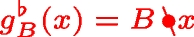 (Brunsch et al. 2012).
Since the functioning of P-TPNs is here reported only to present P-time event graphs, we will not delve into the nuances of weak and strong semantics for P-TPNs. For a thorough description of different types of semantics, we invite the reader to consult (Boyer and Roux 2008).
The concept of time tags is analogous to that of lag times defined as in Baccelli et al. (1992).
Strictly speaking, \(x_i\) is the function that associates to sequence \(w_1w_2\cdots w_k\) the time of the kth occurrence of event i (in mode \(w_k\)). For notational simplicity, however, we prefer to write x(k) in place of \(x(w_1w_2\cdots w_k)\), relying on the fact that the meaning is clear from the context.
In concurrent systems theory, one would say that \(u w_k w_{k+1} v\) and \(u w_{k+1} w_k v\) represent the same trace (Mazurkiewicz 1987).
Note that the trajectory is 1-periodic for the P-TEG.
The problem is written in the max-plus algebra for simplicity. To get the standard linear programming formulation, we refer to Sect. 2.3.2 and recall that \(\lambda _1\otimes \lambda _2\) coincides with \(\lambda _1 + \lambda _2\).
Recall that discrete-time switched linear systems follow \(x(k+1) = A^1_{w_k} \cdot x(k)\), where \(\cdot \) indicates the standard matrix–vector multiplication.
In this section, \(u_{hk}\) and \(v_{hk}\) denote the kth mode in subschedules \(u_h\) and \(v_h\), respectively.
 (Baccelli et al.
  (Brunsch et al.
 References
Abate A, Cimatti A, Micheli A, Mufid MS (2020) Computation of the transient in max-plus linear systems via SMT-solving. In: Bertrand N, Jansen N (eds). Formal modeling and analysis of timed systems. Springer International Publishing. pp 161–177
Alsaba M, Lahaye S, Boimond JL (2006) On just in time control of switching max-plus linear systems. In: ICINCO-SPSMC, pp 79–84
Amari S, Demongodin I, Loiseau JJ, Martinez C (2012) Max-plus control design for temporal constraints meeting in timed event graphs. IEEE Trans Autom Control 57(2):462–467. https://doi.org/10.1109/TAC.2011.2164735
Animobono D, Scaradozzi D, Zattoni E, Perdon AM, Conte G (2023) The model matching problem for max-plus linear systems: a geometric approach. IEEE Trans Autom Control 68(6):3581–3587. https://doi.org/10.1109/TAC.2022.3191362
Åström KJ, Wittenmark B (2013) Computer-controlled systems: theory and design. Courier Corporation
Baccelli F, Cohen G, Olsder GJ, Quadrat JP (1992) Synchronization and linearity: an algebra for discrete event systems. John Wiley & Sons Ltd
Becha T, Hamri H, Kara R, Collart-Dutilleul S (2017) Model predictive control of an electroplating line without stopping the production. Int J Adv Manuf Technol 91:4095–4105
Blyth TS, Janowitz MF (eds) (1972) Residuation theory, vol 102 of international series of monographs on pure and applied mathematics. Pergamon. https://www.sciencedirect.com/science/article/pii/B9780080164083500012
Bonhomme P (2013) Towards a new schedulability technique of real-time systems modeled by P-time Petri nets. Int J Adv Manuf Technol 67:759–769
Boyer M, Roux OH (2008) On the compared expressiveness of arc, place and transition time Petri nets. Fundam Informaticae 88(3):225–249
Brunsch T, Hardouin L, Maia CA, Raisch J (2012) Duality and interval analysis over idempotent semirings. Linear Algebra Appl 437(10):2436–2454
Butkovič P (2010) Max-linear systems: theory and algorithms. Springer Science & Business Media
Calvez S, Aygalinc P, Khansa W (1997) P-time Petri nets for manufacturing systems with staying time constraints. IFAC Proc 30(6):1487–1492
Cuninghame-Green RA (1979) Minimax algebra, vol 166. Springer Science & Business Media
Declerck P (2016) Compromise approach for predictive control of timed event graphs with specifications defined by P-time event graphs. Discrete Event Dyn Syst 26:611–632
Declerck P (2021) Critical subsystems in time interval models. Discrete Event Dyn Syst 31(1):25–35
Declerck P, Guezzi A, Boimond JL (2007) Cycle time of P-time event graphs. In: ICINCO-ICSO, pp 489–496
Fröhlich R, Steneberg SC (2011) Transient multiple hoist scheduling of consecutive cyclic schedules. In: 2011 IEEE international conference on automation science and engineering, pp 357–362
Gaubert S (1995) Resource optimization and (min,+) spectral theory. IEEE Trans Autom Control 40(11):1931–1934
Gaubert S (1995) Performance evaluation of (max,+) automata. IEEE Trans Autom Control 40(12):2014–2025. https://doi.org/10.1109/9.478227
Gaubert S, Mairesse J (1999) Modeling and analysis of timed Petri nets using heaps of pieces. IEEE Trans Autom Control 44(4):683–697
Gonçalves VM, Maia CA, Hardouin L, (2017) On max-plus linear dynamical system theory: the regulation problem. Automatica 75:202–209. https://doi.org/10.1016/j.automatica.2016.09.019
Hardouin L, Cottenceau B, Shang Y, Raisch J (2018) Control and state estimation for max-plus linear systems. Foundations Trends® Syst Control 6(1):1–116
Hecker FT, Stanke M, Becker T, Hitzmann B (2014) Application of a modified GA, ACO and a random search procedure to solve the production scheduling of a case study bakery. Expert Syst Appl 41(13):5882–5891
Hougardy S (2010) The Floyd-Warshall algorithm on graphs with negative cycles. Inf Process Lett 110(8):279–281. https://doi.org/10.1016/j.ipl.2010.02.001
Jungers R (2009) The joint spectral radius: theory and applications, vol 385. Springer Science & Business Media
Karp RM (1978) A characterization of the minimum cycle mean in a digraph. Discrete Math 23(3):309–311. https://doi.org/10.1016/0012-365X(78)90011-0
Kats V, Levner E (2002) Cyclic scheduling in a robotic production line. J Scheduling 5(1):23–41
Kats V, Lei L, Levner E (2008) Minimizing the cycle time of multiple-product processing networks with a fixed operation sequence, setups, and time-window constraints. Eur J Oper Res 187(3):1196–1211. https://doi.org/10.1016/j.ejor.2006.07.030
Katz RD (2007) Max-Plus \((A, B)\)-Invariant spaces and control of timed discrete-event systems. IEEE Trans Autom Control 52(2):229–241. https://doi.org/10.1109/TAC.2006.890478
Khansa W, Denat JP, Collart-Dutilleul S (1996) P-time Petri nets for manufacturing systems. Int Workshop Discrete Event Syst, WODES 96:94–102
Kim JH, Lee TE, Lee HY, Park DB (2003) Scheduling analysis of time-constrained dual-armed cluster tools. IEEE Trans Semicond Manuf 16(3):521–534
Komenda J, Lahaye S, Boimond JL (2009) Supervisory control of (max,+) automata: a behavioral approach. Discrete Event Dyn Syst 19:525–549
Komenda J, Lai A, Godoy Soto J, Lahaye S, Boimond J (2020) Modeling of safe time Petri nets by interval weighted automata. IFAC-Papers OnLine. 15th IFAC Workshop on Discrete Event Systems (WODES) 53(4):187–192. https://doi.org/10.1016/j.ifacol.2021.04.018
Lee JH, Lee TE (2012) Scheduling transient periods of single-armed cluster tools. In: 2012 IEEE international conference on robotics and automation, pp 5062–5067
Lee TE, Park SH, Jung C (2014) Steady state analysis of timed event graphs with time window constraints. Discrete Appl Math 167:202–216
Levner E, Kats V, De Pablo DAL, Cheng TE (2010) Complexity of cyclic scheduling problems: a state-of-the-art survey. Comput Ind Eng 59(2):352–361
Maia CA, Hardouin L, Santos-Mendes R, Loiseau JJ (2011) A super-eigenvector approach to control constrained max-plus linear systems. In: 2011 50th IEEE conference on decision and control and European control conference. IEEE, pp 1136–1141
Maia CA, Andrade C, Hardouin L (2011) On the control of max-plus linear system subject to state restriction. Automatica 47(5):988–992
Manier MA, Bloch C (2003) A classification for hoist scheduling problems. Int J Flex Manuf Syst 15:37–55
Mayer E, Raisch J (2004) Time-optimal scheduling for high throughput screening processes using cyclic discrete event models. Math Comput Simul 66(2–3):181–191
Mazurkiewicz A (1987) Trace theory. In: Petri Nets: applications and relationships to other models of concurrency: advances in Petri Nets 1986, part II proceedings of an advanced course bad Honnef, 8–19, September 1986. Springer, pp 278–324
Nowak T, Charron-Bost B (2014) An overview of transience bounds in max-plus algebra. Trop Idempotent Math Appl 616:277–289
Solomon MM, Desrosiers J (1988) Survey paper-time window constrained routing and scheduling problems. Transp Sci 22(1):1–13
Špaček P, Komenda J (2010) Modeling of interval P-time Petri nets using dioid algebra. IFAC Proc 43(12):312–317
Špaček P, Komenda J (2017) Analysis of cycle time in interval P-time event graphs in dioid algebras. IFAC-PapersOnLine 50(1):13461–13467
Špaček P, Manier MA, Moudni AE (1999) Control of an electroplating line in the max and min algebras. Int J Syst Sci 30(7):759–778
Tavakolipour H, Shakeri F (2018) On tropical eigenvalues of tridiagonal Toeplitz matrices. Linear Algebra Appl 539:198–218
van den Boom TJJ, De Schutter B (2006) Modelling and control of discrete event systems using switching max-plus-linear systems. Control Eng Pract 14(10):1199–1211. https://doi.org/10.1016/j.conengprac.2006.02.006
Watanabe S, Fukuda A, Shigitani H, Iwasaki M (2018) Min-plus eigenvalue of tridiagonal matrices in terms of the ultradiscrete Toda equation. J Phys A: Math Theor 51(44):444001
Zorzenon D, Komenda J, Raisch J (2022) Periodic trajectories in P-time event graphs and the non-positive circuit weight problem. IEEE Control Syst Lett 6:686–691. https://doi.org/10.1109/LCSYS.2021.3085521
Zorzenon D, Komenda J, Raisch J (2022) The non-positive circuit weight problem in parametric graphs: a solution based on dioid theory. Discrete Appl Math 315:56–70
Zorzenon D, Komenda J, Raisch J (2020) Bounded consistency of P-time event graphs. In: 2020 59th IEEE conference on decision and control (CDC), pp 79–85
Zorzenon D, Komenda J, Raisch J (2022) Switched max-plus linear-dual inequalities: application in scheduling of multi-product processing networks. IFAC-PapersOnLine 55(28):196–203. 16th IFAC Workshop on Discrete Event Systems WODES 2022. https://doi.org/10.1016/j.ifacol.2022.10.343
Zorzenon D, Zaiets N, Raisch J (2023) Switched max-plus linear-dual inequalities for makespan minimization: the case study of an industrial bakery shop. IFAC-PapersOnLine 56(2):8628–8634. https://doi.org/10.1016/j.ifacol.2023.10.038
Acknowledgements
We would like to thank Angelos Koumpis for implementing in C MEX a cache-aware max-plus matrix multiplication, which helped achieving the computational time shown in Fig. 13. This work was funded by the Deutsche Forschungsgemeinschaft (DFG, German Research Foundation), Projektnummer RA 516/14-1. Partially supported by RVO 67985840, by the GACR grant 19-06175J, and by Deutsche Forschungsgemeinschaft (DFG, German Research Foundation) under Germany’s Excellence Strategy – EXC 2002/1 "Science of Intelligence" – project number 390523135.
Funding
Open Access funding enabled and organized by Projekt DEAL.
Author information
Authors and Affiliations
Corresponding author
Ethics declarations
Conflict of interest
The authors have no conflict of interest to declare that are relevant to this article.
Additional information
Publisher's Note
Springer Nature remains neutral with regard to jurisdictional claims in published maps and institutional affiliations.
Appendices
Appendix 1 Proof of Proposition 5
Let us consider SLDIs \(\mathcal {S}\) under schedule \(w = v^{+\infty }\), where \(v = v_1v_2\ldots v_V\): for all \(k\in \mathbb {N}\),
By defining
and using Proposition 2, it is possible to rewrite the SLDIs above as the following LDIs: for all \(k\in \mathbb {N}\),
where
Hence, since SLDIs under periodic schedule \(v^{+\infty }\) are equivalent to the above LDIs, according to Theorem 3 they are boundedly consistent if and only if they admit, for some \(\lambda \in \mathbb {R}\), a trajectory of the form
observe that such a trajectory is v-periodic as, in terms of dater x, it satisfies the following property:
To find the set \(\Lambda _{{}_{\text {SLDI}}}^{v}(\mathcal {S})\) of admissible periods for the SLDIs under schedule \(v^{+\infty }\), we proceed as in Sect. 2.4, obtaining:
Therefore, the set \(\Lambda _{{}_{\text {SLDI}}}^{v}(\mathcal {S})\) coincides with all the \(\lambda \)’s such that the precedence graph \(\mathcal {G}(\lambda P_v \oplus \lambda ^{-1} I_v \oplus C_v )\) does not contain circuits with positive weight, where
\(P_h = B_{v_h}^{1\sharp }\), \(I_h = A_{v_h}^1\), and \(C_h = A_{v_h}^0\oplus B_{v_h}^{0\sharp }\) for all \(h\in [\![1,V]\!]\).
Appendix 2 Proof of Theorem 6
In this section, we prove Theorem 6. All symbols used in the following propositions are as in Proposition 5 and Theorem 6. To prove the theorem, we first need a number of technical propositions and lemmas, which provide closed formulas for the computation of elements of the Kleene star of particular sparse matrices. We start from recalling some properties of the Kleene star operation in the max-plus algebra.
Proposition 9
Baccelli et al. (1992) Given two matrices \(a,b\in {\mathbb {R}}_{ \text{ max }}^{n\times n}\), the following properties hold:
Some of the following intermediate results have already been concisely proven in Zorzenon et al. (2022); here we provide a more detailed proof for the first of them.
Lemma 10
Zorzenon et al. (2022) Let \(a\in {\mathbb {R}}_{ \text{ max }}^{n_1\times n_1}\), \(b\in {\mathbb {R}}_{ \text{ max }}^{n_1\times n_2}\), \(c\in {\mathbb {R}}_{ \text{ max }}^{n_2\times n_1}\), and \(d\in {\mathbb {R}}_{ \text{ max }}^{n_2\times n_2}\). Then
Proof
The lemma is proven by applying the formulas from the latter proposition to Algorithm 2 from Hardouin et al. (2018), which can be used for the computation of the Kleene star.
Let \(M^* = \begin{bmatrix}a &{} b\\ c &{} d\end{bmatrix}^* = \begin{bmatrix}\mathcal {M}^{11} &{} \mathcal {M}^{12}\\ \mathcal {M}^{21} &{} \mathcal {M}^{22}\end{bmatrix}\), where each \(\mathcal {M}^{ij}\) is a matrix partitioning \(M^*\) such that \(\mathcal {M}^{11}\in {\mathbb {R}}_{ \text{ max }}^{n_1\times n_1}\); applying Algorithm 2 of Hardouin et al. (2018), we easily get

where \(a^+ = a a^*\) and, consequently, \(a^* = a^+ \oplus E_\otimes \). The formula for matrix \(\mathcal {M}^{12}\) can be obtained in a similar way starting from
which comes from Algorithm 2 of Hardouin et al. (2018). Formulas for \(\mathcal {M}^{21}\) and \(\mathcal {M}^{22}\) are directly derived from reasoning about the symmetry of the Kleene star operation. \(\square \)
Let us now divide matrix \(\lambda P_v\oplus \lambda ^{-1}I_v\oplus C_v\) into four blocks, such that the top-left block is \(C_{1}\in {\mathbb {R}}_{ \text{ max }}^{n\times n}\). We will first focus on formulas to compute specific elements of the Kleene star of the bottom-right block of \(\lambda P_v\oplus \lambda ^{-1}I_v \oplus C_v\), which we will denote by M. We use the following notation:
where each \(\mathcal {M}^{ij}\) is an \(n\times n\) matrix. Note that matrix M is a block tridiagonal matrix, i.e., a matrix whose blocks are all \(\mathcal {E}\) except for those in the main diagonal and in the first diagonals above and below the main diagonal. We refer to Tavakolipour and Shakeri (2018); Watanabe et al. (2018) for some work related to tridiagonal matrices in the tropical (i.e., either max-plus or min-plus) algebra.
Lemma 11
Zorzenon et al. (2022) \(\mathcal {M}^{22} = C_2^* (\mathbb {C}_2^{P})^* C_2^*\).
Lemma 12
\(\mathcal {M}^{VV} = C_{V}^* (\mathbb {C}_{V-1}^{I})^* C_{V}^*\).
Proof
The proof is done by induction on V. For \(V = 3\), the formula can be obtained directly from Lemma 10:
Suppose now that the formula holds for \(V-1\) with \(V \ge 4\); we prove that it holds also for V. By partitioning matrix M in four blocks, such that the bottom-right block coincides with \(C_V\), from Lemma 10 we get
finally, we can use the induction hypothesis to simplify the latter expression into
\(\square \)
Remark 1
More in general, one can prove that, for all \(i\in [\![2,V]\!]\),
considering \(\mathbb {C}_V^P = \mathbb {C}_{1}^I = \mathcal {E}\).
Lemma 13
\(\mathcal {M}^{2V} = (\mathbb {C}^P_2)^* \mathbb {P}_2 (\mathbb {C}^P_3)^* \mathbb {P}_3 \cdots (\mathbb {C}^P_{V-1})^* \mathbb {P}_{V-1}\).
Proof
The proof is done by induction on V. For \(V = 3\), the formula can be obtained directly from Lemma 10:
Suppose now that the formula holds for \(V-1\) with \(V \ge 4\); we prove that it holds also for V. By partitioning matrix M in four blocks, such that the upper-left block coincides with \(C_2\), from Lemma 10 we get that \(\mathcal {M}^{2V}\) is equal to the rightmost block of matrix
Expanding the expression using the induction hypothesis and Lemma 11, we get

which is the desired formula. \(\square \)
Remark 2
With similar techniques, one can prove that, for all \(V\ge 4\) and for all \(i\in [\![3,V-1]\!]\),
Lemma 14
\(\mathcal {M}^{V2} = (\mathbb {C}_{V-1}^{I})^* \mathbb {I}_{V-1} (\mathbb {C}_{V-2}^{I})^* \mathbb {I}_{V-2} \cdots (\mathbb {C}_{2}^{I})^* \mathbb {I}_{2}\).
Proof
The proof is done by induction on V. For \(V = 3\), the formula can be obtained directly from Lemma 10:
Suppose now that the formula holds for \(V-1\) with \(V \ge 4\); we prove that it holds also for V. By partitioning matrix M in four blocks, such that the bottom-right block coincides with \(C_{V}\), from Lemma 10 we get that \(\mathcal {M}^{V2}\) is equal to the leftmost block of matrix
Expanding the expression using the induction hypothesis, Lemma 12, Eqs. 23, and 24, we can get the desired formula with computations analogous to those in the proof of Lemma 13. \(\square \)
Remark 3
With similar techniques, one can prove that, for all \(V\ge 4\) and for all \(i\in [\![3,V-1]\!]\),
In the next proposition, we focus on the top-left \(n\times n\) block of matrix \((\lambda P_v \oplus \lambda ^{-1} I_v \oplus C_v)^*\); we denote this block by \(N\in \mathbb {R}bar^{n\times n}\).
Proposition 15
\(N = C_1^*(\lambda \mathbb {M}^P \oplus \lambda ^{-1} \mathbb {M}^I \oplus \mathbb {M}^C)^*C_1^*\).
Proof
Partitioning matrix \(\lambda P_v\oplus \lambda ^{-1} I_v \oplus C_v\) into four blocks, such that the top-left block is \(C_1\), Lemma 10 gives us
where the latter step can be obtained from Lemmas 11–14, Eqs. 23, and 24. Finally, the commutativity of \(\oplus \) concludes the proof. \(\square \)

Lumped-node representation of \(\mathcal {G}(\lambda P_v \oplus \lambda ^{-1} I_v \oplus C_v)\) when \(V=5\)
After the technical propositions and lemmas above, we are finally ready to introduce the graphical part of the proof. First of all, it is useful to visualize the structure of \(\mathcal {G}(\lambda P_v \oplus \lambda ^{-1} I_v \oplus C_v)\); the lumped-node representation of Fig. 15 illustrates it in the case \(V = 5\). In this simplified representation, \(\overline{k}\) indicates the set of nodes \([\![(k-1)n+1,kn]\!]\) for any \(k\in [\![1,5]\!]\), and the matrix, say Y, associated to an arc from \(\overline{k}_1\) to \(\overline{k}_2\) indicates that an arc in \(\mathcal {G}(\lambda P_v \oplus \lambda ^{-1} I_v \oplus C_v)\) from node \((k_1-1)n+j\) to node \((k_2-1)n+i\) exists iff \(Y_{ij}\ne -\infty \), and that its weight is equal to \(Y_{ij}\), for all \(i,j\in [\![1,n]\!]\).
Recall that, for a square matrix M such that \(M^* = \begin{bmatrix}\mathcal {M}^{11}&{} \mathcal {M}^{12}\\ \mathcal {M}^{21} &{} \mathcal {M}^{22}\end{bmatrix}\), where \(\mathcal {M}^{ii}\) has dimension \(n_i\times n_i\), \(\mathcal {G}(M)\) does not contain circuits with positive weight visiting any node \(j\in [\![1,n_1]\!]\) (respectively, \(j\in [\![n_1+1,n_2]\!]\)) iff \(\mathcal {G}(\mathcal {M}^{11}) \in \Gamma \) (respectively, \(\mathcal {G}(\mathcal {M}^{22})\in \Gamma \)). We partition the set of circuits of \(\mathcal {G}(\lambda P_v \oplus \lambda ^{-1} I_v \oplus C_v)\) in V subsets as follows: (1) circuits visiting at least one node in \(\overline{1}\), (2) circuits that do not visit any node in \(\overline{1}\), but that visit at least one node in \(\overline{2}\), (3) circuits that do not visit any node in \(\overline{1}\) or \(\overline{2}\), but that visit at least one node in \(\overline{3}\), ..., (V) circuits that do not visit any node in \(\overline{1},\overline{2},\ldots ,\overline{V-1}\), but that visit at least one node in \(\overline{V}\). From Proposition 15, the maximal weights of circuits in the first subset correspond to elements in the diagonal of \(N = C_1^*(\lambda \mathbb {M}^P \oplus \lambda ^{-1} \mathbb {M}^I \oplus \mathbb {M}^C)^*C_1^*\); thus these are non-positive iff \(\mathcal {G}(C_1)\in \Gamma \) and \(\lambda \in \Lambda _{\text {NCP}}({\lambda \mathbb {M}^P\oplus \lambda ^{-1}\mathbb {M}^I\oplus \mathbb {M}^C})\). Let \(k\in [\![2,V-1]\!]\). From Lemma 11, the maximal weights of circuits in the kth subset correspond to elements in the diagonal of \(C_k^*(\mathbb {C}^P_k)^* C_k^*\); thus, these are non-positive iff \(\mathcal {G}(C_k)\in \Gamma \) and \(\mathcal {G}(\mathbb {C}^P_k)\in \Gamma \). As for circuits in the Vth subset, their maximal weights come from the diagonal elements of \(C_{V}^*\), which are finite iff \(\mathcal {G}(C_{V})\in \Gamma \).
Appendix 3 Proof of Proposition 7
Consider SLDIs (6) under intermittently periodic schedule \(w = u_0 v_1^{m_1} u_1 v_2^{m_2} u_2 \cdots v_q^{m_q} u_q\), where \(U_q > 0\) (the case in which \(U_q=0\) is analogous but must be considered separately): for all \(k\in [\![1,U_0]\!]\),Footnote 17
for all \(h\in [\![1,q]\!]\), \(j\in [\![0,m_h-1]\!]\), \(k\in [\![1,V_h]\!]\),
for all \(h\in [\![1,q]\!]\), \(k\in [\![1,U_h]\!]\),
and for all \(h\in [\![1,q]\!]\), \(k\in [\![1,U_h]\!]\) with \((h,k)\ne (q,U_q)\),
To search intermittently periodic trajectories, we substitute Eqs. 13 in 26, obtaining: for all \(h\in [\![1,q]\!]\), \(j\in [\![0,m_h-1]\!]\), \(k\in [\![1,V_h]\!]\),

for all \(h\in [\![1,q]\!]\), \(j\in [\![0,m_h-1]\!]\), \(k\in [\![1,V_h-1]\!]\),

for all \(h\in [\![1,q]\!]\), \(j\in [\![0,m_h-2]\!]\) (\(k = V_h\)),

and, for all \(h\in [\![1,q]\!]\) (\(j = m_h-1\), \(k = V_h\)),
To cancel out the \(\lambda _h^{m_h-1}\)’s from Eq. 32, we perform a change of variables. Let \(\xi :[\![1,U_0 + \left( \sum _{h=1}^{q}V_{h}+U_h\right) ]\!]\rightarrow \mathbb {R}^n\) be defined by: for all \(h\in [\![0,q-1]\!]\), \(k\in [\![\left( \sum _{j=1}^{h}U_{j-1}+V_j\right) +1,\sum _{j=1}^{h+1}U_{j-1}+V_j]\!]\),
and for all \(k\in [\![\left( \sum _{j=1}^{q}U_{j-1}+V_j\right) +1,\left( \sum _{j=1}^{q}U_{j-1}+V_j\right) + U_q]\!]\),
By substituting \(\xi \) into inequalities Eqs. 25, 27–32 and simplifying whenever possible the terms in \(\lambda _j\), we obtain that the above inequalities admit a solution in x and \(\lambda _1,\ldots ,\lambda _q\) if and only if the following inequalities admit a solution in \(\xi \) and \(\lambda _1,\ldots ,\lambda _q\): for all \(h\in [\![0,q]\!]\), \(k\in [\![1,U_h]\!]\),
for all \(h\in [\![0,q]\!]\), \(k\in [\![1,U_h]\!]\), \((h,k)\ne (q,U_q)\),
for all \(h\in [\![1,q]\!]\), \(k\in [\![1,V_h]\!]\),
and for all \(h\in [\![1,q]\!]\) (\(k=V_h\)),
The final step in the proof is to rewrite the inequalities (33-36) in terms of the extended vector
and use Proposition 2 to get the max-plus-linear inequality
where \(A(\lambda _1,\ldots ,\lambda _q)\) is a matrix with \((U_0 + \left( \sum _{h=1}^q V_{h}+U_h\right) )n\) rows and columns. Since only the first power of \(\lambda _1,\ldots ,\lambda _q\) shows up in (33-36), matrix \(A(\lambda _1,\ldots ,\lambda _q)\) has the desired form: \(A(\lambda _1,\ldots ,\lambda _q) = \bigoplus _{h=1}^q (\lambda _h P_h\oplus \lambda _h^{-1}I_h)\oplus C\). Therefore, because of Proposition 1, Eq. 37 translates into an MPIC-NCP.
Appendix 4 Proof of Theorem 8

Lumped-node representation of \(\mathcal {G}(A(\lambda _1,\lambda _2))\) from Eq. 16
For notational simplicity, we show how to prove the theorem for the matrix in Eq. 16; the extension to the general case is simple but cumbersome.

Lumped-node representation of \(\mathcal {G}(\overline{A}(\lambda _1,\lambda _2))\) from Eq. 38
First of all, it is useful to draw the parametric precedence graph \(\mathcal {G}(A(\lambda _1,\lambda _2))\) using the lumped-node representation (which was presented in Appendix 2); the graph is shown in Fig. 16. We recall that the objective is to describe in a more compact way the set \(\Lambda _{{}_{\text {NCP}}}(A(\lambda _1,\lambda _2))\) of all parameters \((\lambda _1,\lambda _2)\) for which \(\mathcal {G}(A(\lambda _1,\lambda _2))\) does not contain circuits with positive weight. Before illustrating the proof, it is convenient to relabel the nodes of \(\mathcal {G}(A(\lambda _1,\lambda _2))\) as in Fig. 17; the graph in Fig. 17 therefore corresponds to the precedence graph \(\mathcal {G}(\overline{A}(\lambda _1,\lambda _2))\), where \(\overline{A}\) is obtained permuting rows and columns of \(A(\lambda _1,\lambda _2)\) as follows:

Clearly, \(\mathcal {G}(A(\lambda _1,\lambda _2))\in \Gamma \) if and only if \(\mathcal {G}(\overline{A}(\lambda _1,\lambda _2))\in \Gamma \). We partition matrix \(\overline{A}(\lambda _1,\lambda _2)\) in four blocks, as shown in Eq. 38, and we use the notation
where a and \(\mathcal {M}^{11}\) are matrices of dimension \(10\times 10\) (in general, \(qn\times qn\)). Note that only blocks b and c depend on \(\lambda _1\) and \(\lambda _2\), whereas a and d are numerical matrices.
Then, we partition the set of circuits in \(\mathcal {G}(\overline{A}(\lambda _1,\lambda _2))\) in two subsets:
-
1.
the set of all circuits that do not pass through any node in \(\overline{1}\cup \overline{2}\),
-
2.
the set containing all remaining circuits.
It is easy to see that there are no circuits with positive weight among those in the first subset if and only if \(\mathcal {G}(d)\in \Gamma \); due to the block tridiagonal structure of matrix d, verifying whether \(\mathcal {G}(d)\) contains circuits with positive weight can be done in linear time in the length of \(u_0,\ldots ,u_q\), \(v_1,\ldots ,v_q\) (i.e., the lengths of subschedules \(\textsf{i}\), \(\mathsf {\MakeLowercase {P}}_1\mathsf {\MakeLowercase {P}}_1\mathsf {\MakeLowercase {P}}_3\mathsf {\MakeLowercase {P}}_2\mathsf {\MakeLowercase {P}}_4\), and \(\mathsf {\MakeLowercase {P}}_1\mathsf {\MakeLowercase {P}}_3\mathsf {\MakeLowercase {P}}_2\mathsf {\MakeLowercase {P}}_4\)) using the methods seen in Appendix 2 (or, equivalently, in Zorzenon et al. 2022, Theorem 3).
As for the second subset of circuits, they all visit at least one node in \(\overline{1}\cup \overline{2}\); therefore, their weight is non-positive if and only if \(\mathcal {G}(\mathcal {M}^{11})\in \Gamma \). We can compute \(\mathcal {M}^{11}\) using Lemma 10:
Therefore, \(\mathcal {G}(\mathcal {M}^{11})\in \Gamma \) if and only if
-
1.
\(\mathcal {G}(a)\in \Gamma \),
-
2.
\(\mathcal {G}(a^* bd^* ca^*)\in \Gamma \).
Since \(a = \begin{bmatrix} C_{\mathsf {\MakeLowercase {P}}_1} &{} \mathcal {E}\\ \mathcal {E} &{} C_{\mathsf {\MakeLowercase {P}}_2} \end{bmatrix}\), the first condition is equivalent to having \(\mathcal {G}(C_{\mathsf {\MakeLowercase {P}}_1})\in \Gamma \) and \(\mathcal {G}(C_{\mathsf {\MakeLowercase {P}}_2})\in \Gamma \) (more generally, one has to check the non-positiveness of the circuits in q precedence graphs, each of which contains n nodes).
To check the second condition, we must compute \(a^* bd^* ca^*\). The main challenge here is to find a closed formula for
which can be obtained by using Remarks 1, 2, and 3; the computation takes linear time complexity in the length of subschedules \(u_0,\ldots ,u_q\), \(v_0,\ldots ,v_q\). The resulting matrix \(a^* bd^* ca^*\), of the form \(\lambda _1 P_1 \oplus \lambda _1^{-1} I_1 \oplus \lambda _2 P_2 \oplus \lambda _2^{-1} I_2 \oplus C\) (in general \(\bigoplus _{i=1}^q \lambda _i P_i \oplus \lambda _i^{-1} I_i \oplus C\)), has a number of rows and columns equal to 10 (in general qn). In conclusion, we reduced an MPIC-NCP on a graph with 75 nodes (in general, \((U_0+\sum _{i=1}^q V_i + U_i)n\) nodes) to another MPIC-NCP on a graph with only 10 nodes (in general, pn nodes).
Rights and permissions
Open Access This article is licensed under a Creative Commons Attribution 4.0 International License, which permits use, sharing, adaptation, distribution and reproduction in any medium or format, as long as you give appropriate credit to the original author(s) and the source, provide a link to the Creative Commons licence, and indicate if changes were made. The images or other third party material in this article are included in the article’s Creative Commons licence, unless indicated otherwise in a credit line to the material. If material is not included in the article’s Creative Commons licence and your intended use is not permitted by statutory regulation or exceeds the permitted use, you will need to obtain permission directly from the copyright holder. To view a copy of this licence, visit http://creativecommons.org/licenses/by/4.0/.
About this article

Cite this article
Zorzenon, D., Komenda, J. & Raisch, J. Switched max-plus linear-dual inequalities: cycle time analysis and applications. Discrete Event Dyn Syst 34, 199–250 (2024). https://doi.org/10.1007/s10626-023-00389-5
Received:
Accepted:
Published:
Issue Date:
DOI: https://doi.org/10.1007/s10626-023-00389-5