
Abstract
Presently there is growing interest in dynamic stochastic general equilibrium (DSGE) models with more parameters, endogenous variables, exogenous shocks, and observable variables than the Smets and Wouters (Am Econ Rev 97(3):586–606, 2007) model, and the incorporation of non-Gaussian distribution and time-varying volatility. A primary goal of this paper is to introduce a user-friendly MATLAB toolkit designed to reliably estimate such high-dimensional models. It simulates the posterior distribution by the tailored random block Metropolis-Hastings (TaRB-MH) algorithm of Chib and Ramamurthy (J Econom 155(1):19–38, 2010), calculates the marginal likelihood by the method of Chib (J Am Stat Assoc 90:1313–1312, 1995) and Chib and Jeliazkov (J Am Stat Assoc 96(453):270–281, 2001), and includes various post-estimation tools that are important for policy analysis, for example, functions for generating point and density forecasts. We also introduce two novel features, i.e., tailoring-at-random-frequency and parallel computing, to boost the overall computational efficiency. Another goal is to provide pointers on the prior, estimation, and comparison of these DSGE models. To demonstrate the performance of our toolkit, we apply it to estimate an extended version of the new Keynesian model of Leeper et al (Am Econom Rev 107(8):2409–2454, 2017) that has 51 parameters, 21 endogenous variables, 8 exogenous shocks, 8 observable variables, and 1494 non-Gaussian and nonlinear latent variables.


Code Availability
The toolkit is publicly available at https://github.com/econdojo/dsge-svt.
Notes
The toolkit is publicly available at https://github.com/econdojo/dsge-svt. The results reported in this paper can be replicated by running the program demo.m.
It is straightforward to introduce, as in Cúrdia et al. (2014), an independent Student-t distribution with different degrees of freedom for each shock innovation. For exhibition ease, we do not consider this generalization.
Because some parameters are held fixed under each regime, effectively, \(\theta \) has 49 elements and \(\theta ^S\) has 25 elements.
In the Leeper et al. (2017) setting with Gaussian shocks and constant volatility, this step suggests that the original prior for the standard deviation parameters should be adjusted. Alternatively, one could also adjust other components of the prior for \(\theta ^S\).
The same optimization procedure is applied to obtain a starting value \(\theta ^{S,(0)}\) for the chain. This procedure is repeated multiple times, each of which is initialized at a high density point out of a large number of prior parameter draws. The optimization results will be stored in the MATLAB data file chaininit.mat, which is saved to the subfolder user/ltw17.
It is worth noting that the total runtime for generating 11,000 draws is about 30 hours for \(\omega =0.5\) and is about 43 hours for \(\omega =1.0\). These numbers were measured based on a computer with Intel (R) i5-6500 CPU with 16 GB RAM. With an average inefficiency factor of 14.46 for \(\omega =0.5\) and 15.66 for \(\omega =1.0\), these numbers translate into 25.36 and 16.34 i.i.d.-equivalent draws per hour, respectively. This comparison exemplifies that the tailoring-at-random-frequency feature can effectively improve the computational efficiency of the TaRB-MH algorithm.
Fig. 4 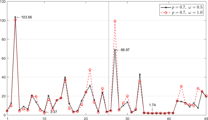
Inefficiency factor of each parameter. Notes: The horizontal axis indicates parameter indices. The vertical line separates the structural (indexed by 1–25) and volatility (indexed by 26–49) parameters
The DGPs for the structural parameters correspond to their full sample (1955:Q1–2014:Q2) regime-M estimates reported in Leeper et al. (2017).
For instance, the modified harmonic mean (MHM) estimator of Gelfand and Dey (1994), used, for example, in Justiniano and Primiceri (2008) and Cúrdia et al. (2014) in medium-scale DSGE models with Student-t shocks and stochastic volatility, always favors a model specification with stronger latent features, e.g., shocks with fatter tails or volatilities with more persistence. This extreme result emerges even when the true model exhibits weak evidence of these features, such as those considered in Sect. 5.3.
In contrast, Justiniano and Primiceri (2008, p. 636) and Herbst and Schorfheide (2016, p. 97) estimate the posterior ordinate in a single block, with the random-walk M-H, both detrimental to getting reliable and efficient marginal likelihood estimates, as already documented in Chib and Jeliazkov (2001).
All computations performed in this section are executed on the High Performance Computing Cluster maintained by Saint Louis University (https://slu.zendesk.com/hc).
This density function, when it is evaluated at the realized value of \(y_{T+1:T+h}|y_{1:T}\), is called a predictive likelihood. It is oftentimes used for comparing different models [see, e.g., Chib and Greenberg (1995a)].
Define the parameter \(0<\psi <1\) such that \(\frac{\Psi ''(1)}{\Psi '(1)}\equiv \frac{\psi }{1-\psi }\).
\(S(\cdot )\) satisfies \(S'(e^{\gamma })=0\) and \(S''(e^{\gamma })\equiv s>0\).
See the Online Appendix of Leeper et al. (2017) for details on data construction.

References
Born, B., & Pfeifer, J. (2014). Policy risk and the business cycle. Journal of Monetary Economics, 68, 68–85.
Champagne, J., & Kurmann, A. (2013). The great increase in relative wage volatility in the United States. Journal of Monetary Economics, 60(2), 166–183.
Chan, J. C., & Grant, A. L. (2015). Pitfalls of estimating the marginal likelihood using the modified harmonic mean. Economics Letters, 131, 29–33.
Chen, R., & Liu, J. S. (2000). Mixture Kalman filters. Journal of the Royal Statistical Society: Series B (Statistical Methodology), 62(3), 493–508.
Chib, S. (1995). Marginal likelihood from the Gibbs output. Journal of the American Statistical Association, 90, 1313–1321.
Chib, S., & Ergashev, B. (2009). Analysis of multifactor affine yield curve models. Journal of the American Statistical Association, 104(488), 1324–1337.
Chib, S., & Greenberg, E. (1995a). Hierarchical analysis of SUR models with extensions to correlated serial errors and time-varying parameter models. Journal of Econometrics, 68(2), 339–360.
Chib, S., & Greenberg, E. (1995b). Understanding the metropolis-hastings algorithm. The American Statistician, 49(4), 327–335.
Chib, S., & Jeliazkov, I. (2001). Marginal likelihood from the metropolis-hastings output. Journal of the American Statistical Association, 96(453), 270–281.
Chib, S., Nardari, F., & Shephard, N. (2002). Markov chain Monte Carlo methods for stochastic volatility models. Journal of Econometrics, 108(2), 281–316.
Chib, S., & Ramamurthy, S. (2010). Tailored randomized block MCMC methods with application to DSGE models. Journal of Econometrics, 155(1), 19–38.
Chib, S., & Ramamurthy, S. (2014). DSGE models with student-t errors. Econometric Reviews, 33(1–4), 152–171.
Chib, S., & Zeng, X. (2020). Which Factors are risk factors in asset pricing? A model scan framework. Journal of Business & Economic Statistics, 38(4), 771–783.
Chiu, C.-W.J., Mumtaz, H., & Pinter, G. (2017). Forecasting with VAR models: Fat tails and stochastic volatility. International Journal of Forecasting, 33(4), 1124–1143.
Cúrdia, V., Del Negro, M., & Greenwald, D. L. (2014). Rare shocks, great recessions. Journal of Applied Econometrics, 29(7), 1031–1052.
Dave, C., & Malik, S. (2017). A tale of fat tails. European Economic Review, 100, 293–317.
Diebold, F. X., Schorfheide, F., & Shin, M. (2017). Real-time forecast evaluation of DSGE models with stochastic volatility. Journal of Econometrics, 201(2), 322–332.
Durbin, J., & Koopman, S. J. (2002). A simple and efficient simulation smoother for state space time series analysis. Biometrika, 89(3), 603–615.
Franta, M. (2017). Rare shocks vs. non-linearities: What drives extreme events in the economy? Some empirical evidence. Journal of Economic Dynamics & Control, 75, 136–157.
Gelfand, A. E., & Dey, D. K. (1994). Bayesian model choice: Asymptotics and exact calculations. Journal of the Royal Statistical Society Series B (Methodological), 56(3), 501–514.
Geweke, J. F. (2005). Contemporary Bayesian Econometrics and Statistics. Wiley.
Herbst, E. P., & Schorfheide, F. (2016). Bayesian Estimation of DSGE Models. Princeton University Press.
Justiniano, A., & Primiceri, G. E. (2008). The time-varying volatility of macroeconomic fluctuations. American Economic Review, 98(3), 604–41.
Kapetanios, G., Masolo, R. M., Petrova, K., & Waldron, M. (2019). A time-varying parameter structural model of the UK economy. Journal of Economic Dynamics & Control, 106, 103705.
Kim, S., Shephard, N., & Chib, S. (1998). Stochastic volatility: Likelihood inference and comparison with ARCH models. The Review of Economic Studies, 65(3), 361–393.
Kim, Y. M., & Kang, K. H. (2019). Likelihood inference for dynamic linear models with Markov switching parameters: On the efficiency of the Kim filter. Econometric Reviews, 38(10), 1109–1130.
Kulish, M., Morley, J., & Robinson, T. (2017). Estimating DSGE models with zero interest rate policy. Journal of Monetary Economics, 88, 35–49.
Lazarus, E., Lewis, D. J., Stock, J. H., & Watson, M. W. (2018). HAR inference: Recommendations for practice. Journal of Business & Economic Statistics, 36(4), 541–559.
Leeper, E. M., Traum, N., & Walker, T. B. (2017). Clearing up the fiscal multiplier morass. American Economic Review, 107(8), 2409–54.
Liu, X. (2019). On tail fatness of macroeconomic dynamics. Journal of Macroeconomics, 62, 103154.
Mele, A. (2020). Does school desegregation promote diverse interactions? An equilibrium model of segregation within schools. American Economic Journal-Economic Policy, 12(2), 228–257.
Rathke, A., Straumann, T., & Woitek, U. (2017). Overvalued: Swedish monteary policy in the 1930s. International Economic Review, 58(4), 1355–1369.
Sims, C. A. (2002). Solving linear rational expectations models. Computational Economics, 20(1), 1–20.
Sims, C. A., Waggoner, D. F., & Zha, T. (2008). Methods for inference in large multiple-equation Markov-switching models. Journal of Econometrics 146(2), 255–274. Nelson: Honoring the research contributions of Charles R.
Smets, F., & Wouters, R. (2007). Shocks and frictions in US business cycles: A Bayesian DSGE approach. American Economic Review, 97(3), 586–606.
Funding
F. Tan acknowledges the financial support from the Chaifetz School of Business summer research grant.
Author information
Authors and Affiliations
Corresponding author
Ethics declarations
Conflicts of interest
The authors declare that they have no conflict of interest.
Additional information
Publisher's Note
Springer Nature remains neutral with regard to jurisdictional claims in published maps and institutional affiliations.
The views expressed in this paper are solely those of the authors and do not necessarily reflect the views of the Federal Reserve Bank of Philadelphia or the Federal Reserve System.
Appendices
Appendix A: Leeper-Traum-Walker Model
1.1 Linearized System
Unless otherwise noted, we let \({\hat{x}}_t\equiv \ln x_t-\ln x\) denote the log-deviation of a generic variable \(x_t\) from its steady state x. We also divide a non-stationary variable \(X_t\) by the level of technology \(A_t\) and express the detrended variable as \(x_t=X_t/A_t\).
1.1.1 Firms
The production sector consists of firms that produce intermediate and final goods. A perfectly competitive final goods producer uses intermediate goods supplied by a continuum of intermediate goods producers indexed by i on the interval [0, 1] to produce the final goods. The production technology \(Y_t\le \left( {\int ^1_0}Y_t(i)^{1/(1+\eta ^p_t)}di\right) ^{1+\eta ^p_t}\) is constant-return-to-scale, where \(\eta ^p_t\) is an exogenous price markup shock, \(Y_t\) is the aggregate demand of final goods, and \(Y_t(i)\) is the intermediate goods produced by firm i.
Each intermediate goods producer follows a production technology \(Y_t(i)=K_t(i)^{\alpha }\left( A_{t}L^d_t(i)\right) ^{1-\alpha }-A_t \Omega \), where \(K_t(i)\) and \(L^d_t(i)\) are the capital and the amount of ‘packed’ labor input rented by firm i at time t, and \(0<\alpha <1\) is the income share of capital. \(A_t\) is the labor-augmenting neutral technology shock and its growth rate \(u^a_t\equiv \text {ln}(A_t/A_{t-1})\) equals \(\gamma >0\) when \(A_t\) evolves along the balanced growth path. The parameter \(\Omega >0\) represents the fixed cost of production.
Intermediate goods producers maximize their profits in two stages. First, they take the input prices, i.e., nominal wage \(W_t\) and nominal rental rate of capital \(R^k_t\), as given and rent \(L^d_t(i)\) and \(K_t(i)\) in perfectly competitive factor markets. Second, they choose the prices that maximize their discounted real profits. Here we introduce the Calvo-pricing mechanism for nominal price rigidities. Specifically, a fraction \(0<\omega _p<1\) of firms cannot change their prices each period. All other firms can only partially index their prices by the rule \(P_t(i)=P_{t-1}(i)\left( \pi _{t-1}^{\chi _p}\pi ^{1-\chi _p}\right) \), where \(P_{t-1}(i)\) is indexed by the geometrically weighted average of past inflation \(\pi _{t-1}\) and steady state inflation \(\pi \). The weight \(0<\chi _p<1\) controls the degree of partial indexation.
The production sector can be summarized by four log-linearized equilibrium equations in terms of six parameters \((\alpha ,\Omega ,\beta ,\omega _p,\chi _p,\eta ^p)\), seven endogenous variables \(({\hat{y}}_t,{\hat{k}}_t,{\hat{L}}_t,{\hat{r}}_t^k,{\hat{w}}_t,{\widehat{mc}}_t,{\hat{\pi }}_t)\), and one exogenous shock \({\hat{u}}_t^p\):
where \(\kappa _p\equiv [(1-\beta \omega _p)(1-\omega _p)]/[\omega _p(1+\beta \chi _p)]\), \({\hat{\eta }}^p_t\equiv \ln (1+\eta ^p_t)-\ln (1+\eta ^p)\), \({\hat{\eta }}^p_t\) is normalized to \({\hat{u}}^p_t\equiv \kappa _p{\hat{\eta }}^p_t\), and \({\mathbb {E}}_t\) represents mathematical expectation given information available at time t.
1.1.2 Households
The economy is populated by a continuum of households indexed by j on the interval [0, 1]. Each optimizing household j derives utility from composite consumption \(C_t^*(j)\), relative to a habit stock defined in terms of lagged aggregate composite consumption \(hC_{t-1}^*\) where \(0<h<1\). The composite consumption consists of private \(C_t(j)\) and public \(G_t\) consumption goods, i.e., \(C_t^{*}(j){\equiv }C_t(j)+\alpha _{G}G_t\), where \(\alpha _G\) governs the degree of substitutability of the consumption goods. Each household j also supplies a continuum of differentiated labor services \(L_t(j,l)\) where \(l\in [0,1]\). Households maximize their expected lifetime utility \({\mathbb {E}}_0 \overset{\infty }{\underset{t=0}{\sum }} \beta ^t u^b_t \left[ \text {ln}(C_t^*(j)-hC_{t-1}^*)-L_t(j)^{1+\xi }/(1+\xi )\right] \), where \(0<\beta <1\) is the discount rate, \(\xi >0\) is the inverse of Frisch labor supply elasticity, and \(u^b_t\) is an exogenous preference shock.
Households have access to one-period nominal private bonds \(B_{s,t}\) that pay one unit of currency at time \(t+1\), sell at price \(R_t^{-1}\) at time t, and are in zero net supply. They also have access to a portfolio of long-term nominal government bonds \(B_t\), which sell at the price \(P^B_t\) at time t. Maturity of these zero-coupon bonds decays at the constant rte \(0<\rho <1\) to yield the average duration \((1-\rho \beta )^{-1}\). Households receive bond earnings, labor and capital rental income, lump-sum transfers from the government \(Z_t\), and profits from firms \(\Pi _t\). They spend income on consumption, investment \(I_t\), and bonds. The nominal flow budget constraint for household j is given by
where \(W_t(l)\) is the nominal wage charged by the household for type l labor service. Consumption and labor income are, in nominal terms, subject to a sales tax \(\tau ^C>0\) and a labor income tax \(\tau ^L>0\), respectively.
Effective capital K(j), which is subject to a rental income tax \(\tau ^K>0\), is related to physical capital \({\bar{K}}(j)\) via \(K_t(j)=v_t(j){\bar{K}}_{t-1}(j)\), where \(v_t(j)\) is the utilization rate of capital chosen by households and incurs a nominal cost of \(\Psi (v_t)\) per unit of physical capital.Footnote 13 Physical capital is accumulated by households according to \({\bar{K}}_{t}(j)=(1-\delta ){\bar{K}}_{t-1}(j)+u^i_t\left( 1-S\left( \frac{I_t(j)}{I_{t-1}(j)}\right) \right) I_t(j)\), where \(0<\delta <1\) is the depreciation rate, \(S(\cdot )I_t\) is an investment adjustment cost and \(u_t^i\) is an exogenous investment-specific efficiency shock.Footnote 14
There are perfectly competitive labor packers that hire a continuum of differentiated labor inputs \(L_t(l)\), pack them to produce an aggregate labor service and then sell it to intermediate goods producers. The labor packer uses the Dixit-Stiglitz aggregator for labor aggregation \(L^d_{t}=\left( {\int ^1_0}L_t(l)^{1/(1+\eta ^w_t)}dl\right) ^{1+\eta ^w_t}\), where \(L^d_{t}\) is the aggregate labor service demanded by intermediate goods producers, \(L_t(l)\) is the lth type labor service supplied by all the households and demanded by the labor packer, and \(\eta ^w_t\) is an exogenous wage markup shock.
For the optimal wage setting problem, we adopt the Calvo-pricing mechanism for nominal wage rigidities. Specifically, of all the types of labor services within each household, a fraction \(0<\omega _w<1\) of wages cannot be changed each period. The wages for all other types of labor services follow a partial indexation rule \(W_t(l)=W_{t-1}(l)\left( \pi _{t-1}e^{u^a_{t-1}}\right) ^{\chi _w}\left( \pi e^{\gamma }\right) ^{1-\chi _w}\), where \(W_{t-1}(l)\) is indexed by the geometrically weighted average of the growth rates of nominal wage in the past period and in the steady state, respectively. The weight \(0<\chi _w<1\) controls the degree of partial indexation.
The household sector can be summarized by ten log-linearized equilibrium equations in terms of seventeen parameters \((h,\gamma ,\alpha _G,\rho ,\tau ^C,\tau ^K,\tau ^L,\psi ,\beta ,\gamma ,s,\delta ,\xi ,\omega _w,\chi _w,\rho _a,\eta ^w)\), fifteen endogenous variables \(({\hat{\lambda }}_t,{\hat{c}}_t^*,{\hat{c}}_t,{\hat{g}}_t,{\hat{R}}_t,{\hat{\pi }}_t,{\hat{P}}_t^B,{\hat{r}}_t^k,{\hat{v}}_t,{\hat{q}}_t,{\hat{i}}_t,{\hat{k}}_t,\hat{{\bar{k}}}_t,{\hat{w}}_t,{\hat{L}}_t)\), and four exogenous shocks \(({\hat{u}}_t^a,{\hat{u}}_t^b,{\hat{u}}_t^i,{\hat{u}}_t^w)\):
where \(\kappa _w\equiv [(1-\beta \omega _w)(1-\omega _w)]/[\omega _w(1+\beta )(1+(1/\eta ^w+1)\xi )]\), \({\hat{\eta }}^w_t\equiv \ln (1+\eta ^w_t)-\ln (1+\eta ^w)\), \({\hat{\eta }}^w_t\) is normalized to \({\hat{u}}^w_t\equiv \kappa _w{\hat{\eta }}^w_t\), \(\hat{{\tilde{u}}}^i_t\) is normalized to \({\hat{u}}^i_t\equiv \frac{1}{(1+\beta )s e^{2\gamma }}\hat{{\tilde{u}}}^i_t\), and \(\lambda _t\) is the Lagrange multiplier associated with the household’s budget constraint. We set the capital, labor, and consumption tax rates to their constant steady states so that \({\hat{\tau }}^K_t={\hat{\tau }}^L_t={\hat{\tau }}^C_t=0\).
1.1.3 Monetary and Fiscal Policy
The central bank implements monetary policy according to a Taylor-type interest rate rule. The government collects revenues from capital, labor, and consumption taxes, and sells nominal bond portfolios to finance its interest payments and expenditures. The fiscal choices must satisfy the government budget constraint \(P^B_tB_t+\tau ^KR^K_tK_t+\tau ^LW_tL_t+\tau ^CP_tC_t=(1+\rho P^B_t)B_{t-1}+P_tG_t+P_tZ_t\), where we have assumed the lump sum transfers are equal across households, i.e., \(\int _{0}^{1}Z_t(j)dj=Z_t\), and fiscal instruments follow the simple rules specified below.
The government sector can be summarized by seven log-linearized equilibrium equations in terms of thirteen parameters \((\tau ^C,\tau ^K,\tau ^L,\beta ,\gamma ,\rho ,\rho _r,\rho _g,\rho _z,\phi _{\pi },\phi _y,\gamma _g,\gamma _z)\), sixteen endogenous variables \(({\hat{b}}_t,{\hat{r}}_t^k,{\hat{k}}_t,{\hat{w}}_t,{\hat{L}}_t,{\hat{c}}_t,{\hat{\pi }}_t,{\hat{P}}_t^B,{\hat{g}}_t,{\hat{z}}_t,{\hat{y}}_t,{\hat{i}}_t,{\hat{v}}_t,{\hat{R}}_t,{\hat{s}}_t^b,{\hat{s}}_t)\), and four exogenous shocks \(({\hat{u}}^a_t,{\hat{u}}^m_t,{\hat{u}}^g_{t},{\hat{u}}^z_{t})\):
where \(s^b_{t-1}\equiv \frac{P^B_{t-1}B_{t-1}}{P_{t-1}Y_{t-1}}\) denotes the market value of the debt-to-GDP ratio, \(s=\tau ^K r^k k + \tau ^L w L + \tau ^C c - g - z\), \(0<\rho _r,\rho _g,\rho _z<1\) measure policy smoothness, \(\phi _\pi ,\phi _y>0\) and \(\gamma _g,\gamma _z\) are policy parameters, and \(({\hat{u}}^m_t,{\hat{u}}^g_{t},{\hat{u}}^z_{t})\) are exogenous policy shocks.
1.1.4 Exogenous Processes
All exogenous shocks follow autoregressive processes
where \(\rho _{es}\in (0,1)\) and the innovations \(\epsilon _t^s\) are serially uncorrelated and independent of each other at all leads and lags.
1.2 Original System
Since the economy features a stochastic trend induced by the permanent technology shock \(A_t\), some variables are not stationary. To induce stationarity, we therefore detrend these variables as: \(y_t\equiv \frac{Y_t}{A_t}\), \(c_t^*\equiv \frac{C_t^*}{A_t}\), \(c_t\equiv \frac{C_t}{A_t}\), \(k_t\equiv \frac{K_t}{A_t}\), \({\bar{k}}_t\equiv \frac{{\bar{K}}_t}{A_t}\), \(i_t\equiv \frac{I_t}{A_t}\), \(g_t\equiv \frac{G_t}{A_t}\), \(z_t\equiv \frac{Z_t}{A_t}\), \(b_t\equiv \frac{P^B_{t}B_t}{P_{t}A_t}\), \(w_t\equiv \frac{W_t}{P_{t}A_t}\), \(\lambda _t\equiv \varLambda _{t}A_t\). The model’s equilibrium system in terms of the detrended variables can be summarized as follows.
Production function:
Capital-labor ratio:
Real marginal cost:
Intermediate goods producer’s optimal price:
Evolution of aggregate price index:
Optimal consumption:
Composite consumption:
Consumption Euler equation:
Bond pricing relation:
Optimal capital utilization:
Optimal physical capital:
where \(q_t\) is the real price of capital in terms of consumption goods (i.e., Tobin’s Q).
Optimal investment:
Effective capital:
Law of motion for capital:
Optimal wage:
where
Evolution of aggregate wage index:
Government budget constraint:
Aggregate resource constraint:
1.3 Steady States
To solve for the steady states, we calibrate \(\beta =0.99\), \(\alpha =0.33\), \(\delta =0.025\), the average maturity of government bond portfolio \(AD=20\), \(\eta ^w=\eta ^p=0.14\), \(g/y=0.11\), \(b/y=1.47\), \(\tau ^C=0.023\), \(\tau ^K=0.218\), and \(\tau ^L=0.186\). By assumption, \(v=1\), \(\psi (v)=0\), and \(S(e^\gamma )=S'(e^\gamma )=0\). The remaining steady states can be solved as follows.
From AD:
From (A.30):
From (A.31):
From \({\tilde{u}}^i=1\) and (A.34):
From (A.33):
From (A.32):
From (A.26):
From (A.25):
From (A.24):
From \(\Delta ^p=1\), the final goods producer’s zero profit condition, and (A.23):
From (A.51):
From (A.35):
From (A.36):
From (A.41):
From (A.40):
From (A.29):
from which all level variables can be calculated from the steady state ratios given above.
1.4 Taking Model to Data
Define the private sector’s one-step-ahead endogenous forecast errors as
The model consists of 36 log-linearized equilibrium equations and can be cast into the rational expectations system
where I denotes the identity matrix, \(P=\text {diag}\left( \rho _{ea},\rho _{eb},\rho _{ei},\rho _{ep},\rho _{ew},\rho _{em},\rho _{eg},\rho _{ez}\right) \),
are the endogenous variables,
are the exogenous shocks,
are the conditional expectations of the last seven elements of \(x_{t+1}^{e}\) ,
are the shock innovations, and
are the forecast errors.
Here the first row of (A.60) stacks the 21 structural equations (A.1)– (A.21), the second row stacks the 8 shock processes (A.22), and the third row stacks the 7 definitional equations (A.59). The unknown parameters \(\theta \) consist of the structural parameters
and the volatility parameters
Conditional on \(\theta ^S\) and independent of the volatility processes, the above structural system can be solved by the procedure of Sims (2002) to deliver a linear solution of the form
which is then estimated over a vector \(y_t\) of 8 observable variables stacked in \(y_{1:T}=[y_1,\ldots ,y_T]'\), including log differences (denoted dl) of consumption, investment, real wage, government spending, and government debt; log (denoted l) hours worked, inflation, and nominal interest rate.Footnote 15 The observable variables are linked to the model variables \(x_t\) via the following measurement equations:
Let \(\lambda _{1:T}=[\lambda _1,\ldots ,\lambda _T]'\) contain all non-Gaussian latent states and \(h_{1:T}=[h_1',\ldots ,h_T']'\) contain all nonlinear latent states. In our empirical application (\(T=166\)), \(\lambda _{1:T}\) and \(h_{1:T}\) have a total of 1,494 elements. In conjunction with the shock volatility specifications (2.2) and (2.3), equations (A.61) and (A.62) form a state space representation of the DSGE model whose conditional likelihood function \(f(y_{1:T}|\theta ,\lambda _{1:T},h_{1:T})\) can be evaluated with the Kalman filter.
1.5 Tables and Figures
-
Table 5 lists the marginal prior distributions and the true values for the high-dimensional DSGE model under regime-M.
-
Table 6 summarizes the posterior parameter estimates for the model of best fit.
-
Table 7 reproduces the subsample posterior parameter estimates reported in Leeper et al. (2017), which are used to generate the simulated data sets in Sect. 5.3.
-
Figures 8 and 9 display the autocorrelation function for each model parameter.
-
Figures 10 and 11 compare the model’s estimated parameters and volatilities with their true values, respectively.

Autocorrelation function of each structural parameter. Notes: Red horizontal lines correspond to an autocorrelation of 0.1

Autocorrelation function of each volatility parameter. Notes: See Fig. 8

Marginal prior and posterior distributions of each structural parameter. Notes: Each panel compares the prior (red dashed line) with the posterior (shaded area). Vertical lines denote the true parameter values. The kernel smoothed posterior densities are estimated using 10, 000 TaRB-MH draws

Stochastic volatility of each shock innovation. Notes: Each panel compares the model’s estimated log-variances with their true values (red solid line). Blue dashed lines denote median estimates, while shaded areas delineate \(90\%\) highest posterior density bands
Appendix B: Small-Scale DSGE Model
A log-linear approximation to the model’s equilibrium conditions around the steady state can be summarized as follows:
Here \(\tau >0\) is the coefficient of relative risk aversion, \(0<\beta <1\) is the discount factor, \(\kappa >0\) is the slope of the new Keynesian Phillips curve, \(\psi _1>0\) and \(\psi _2>0\) are the policy rate responsive coefficients, and \(0\le \rho _R,\rho _{z},\rho _g<1\). Moreover, \(c_t\) is the detrended consumption, \(\pi _t\) is the inflation between periods \(t-1\) and t, \(R_t\) is the nominal interest rate, \(z_t\) is an exogenous shock to the labor-augmenting technology that grows on average at the rate \(\gamma \), and \(g_t\) is an exogenous government spending shock. Finally, the shock innovations \(\epsilon _t=[\epsilon _{R,t},\epsilon _{z,t},\epsilon _{g,t}]'\) follow a multivariate Student-t distribution, i.e., \(\epsilon _t\sim t_{\nu }(0,\Sigma _t)\), where \(\Sigma _t=\text {diag}\left( e^{h_t}\right) \) and each element of \(h_t=[h_t^R,h_t^z,h_t^g]'\) follows a stationary process
The model is estimated over three observable variables, including log difference of consumption, log inflation, and log nominal interest rate. The observable variables are linked to the model variables via the following measurement equations,
where \((\gamma ^{(Q)},\pi ^{(Q)},r^{(Q)})\) are connected to the model’s steady states via \(\gamma =1+\gamma ^{(Q)}/100\), \(\beta =1/(1+r^{(Q)}/100)\), and \(\pi =1+\pi ^{(Q)}/100\). Table 8 lists the marginal prior distributions for the small-scale DSGE model parameters.
Appendix C: Practical Guide
The subfolder user/ltw17 contains the following files for the Leeper-Traum-Walker model, which are extensively annotated and can be modified, as needed, for alternative model specifications:
-
user_parvar.m—defines the parameters, priors, variables, shock innovations, forecast errors, and observable variables.
-
user_mod.m—defines the model and measurement equations.
-
user_ssp.m—defines the steady state, implied, and/or fixed parameters.
-
user_svp.m—defines the stochastic volatility parameters.
-
data.txt—prepared in matrix form where each row corresponds to the observations for a given period.
Our MATLAB toolkit is readily deployed. Once the user supplies the above model and data files, the posterior distribution, marginal likelihood, and predictive distributions (and other quantities) are computed via the single function, tarb.m, as will be illustrated below. A printed summary of the results will be recorded in the MATLAB diary file mylog.out, which is saved to the subfolder user/ltw17.
-
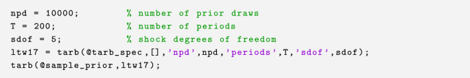
1.
The prior sampling is implemented through the following block of code. The sampling results will be stored in the MATLAB data file tarb_prior.mat, which is saved to the subfolder user/ltw17.
-
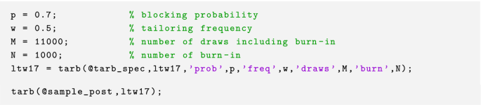
2.
The posterior sampling is implemented in the following block of code. The estimation results will be stored in the MATLAB data file tarb_full.mat, which is saved to the subfolder user/ltw17.
-
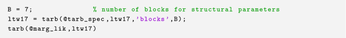
3.
The marginal likelihood estimation is implemented in the following block of code. The estimation results will be stored in the MATLAB data file tarb_reduce.mat, which is saved to the subfolder user/ltw17.
-
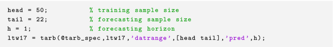
4.
Sampling the predictive distribution is specified in the following block of code.


Rights and permissions
About this article

Cite this article
Chib, S., Shin, M. & Tan, F. DSGE-SVt: An Econometric Toolkit for High-Dimensional DSGE Models with SV and t Errors. Comput Econ 61, 69–111 (2023). https://doi.org/10.1007/s10614-021-10200-y
Accepted:
Published:
Issue Date:
DOI: https://doi.org/10.1007/s10614-021-10200-y
Keywords
- DSGE models
- Bayesian inference
- Marginal likelihood
- Tailored proposal densities
- Random blocks
- Student-t shocks
- Stochastic volatility