A practical probabilistic earthquake hazard analysis tool: case study Marmara region

Abstract

Earthquakes have a damaging impact on the economic welfare and resilience of communities, particularly in developing countries. Seismic hazard assessment is the first step towards performing prevention, preparedness, and response or recovery actions to reduce seismic risk. This paper presents a computation tool for predicting the seismic hazard at the macro level as a part of a comprehensive multi-hazard framework on earthquake risk assessment. The probabilistic seismic hazard analysis (PSHA) procedure is based on the Monte-Carlo approach, and particular attention is paid to the definition of source zones assigned in the study area. Both Poisson and time dependent (renewal) models are adopted to quantify the effect of temporal dependencies between seismic events, while near-field rupture directivity effects are also taken into account. Marmara region in Turkey is selected as a case study area to perform a new seismic hazard analysis and verify the accuracy of the proposed tool. The results show good agreement with results from the recent SHARE project and the latest Turkish Earthquake Design code hazard maps. This confirms that the proposed PSHA method can be an attractive alternative to the direct integration based methods due to its practicality and powerful handling of uncertainties.

1 Introduction

Seismic risk is determined by combining the likelihood of seismic events over a pre-defined timeframe at a specific site or area/region and the consequences of this event on assets in the area. Hence, seismic hazard, vulnerability and value of exposed infrastructure are the main components of earthquake risk assessment (Silva et al. 2015). Whilst the occurrence of earthquakes cannot be predicted accurately, our current understanding of global tectonics and seismology allows us to make reasonable estimates of seismic hazard in most regions of the world. However, detailed seismic risk estimation for a site/area is still a complex task as it requires huge amounts of data such as seismo-tectonic structure, seismicity, soil conditions, building stock and population of the considered area.

The seismic hazard at a site can be quantified by undertaking deterministic or probabilistic seismic hazard analysis (PSHA) (Erdik 2017). In the deterministic approach, a particular earthquake scenario, called controlling earthquake, is used to estimate hazard at a site. On the other hand, PSHA can be used to quantify the probability of exceedance of various ground motion levels at a site/region for different return periods of earthquakes. Contrary to the deterministic approach, the probabilistic approach can take into account all potential earthquake sources with the inclusion of uncertainties arising from earthquake size, location and occurrence time.

Conventional PSHA calculations (e.g. Cornell 1968) are carried out using the total probability theorem, for which the contribution of all possible seismic events along with their associated probability of occurrences are combined. Alternatively, stochastic modelling approaches using Monte-Carlo (MC) simulation method can be used to generate synthetic earthquake catalogues by randomizing key parameters (in a controlled way) obtained from past seismicity, tectonic settings and geological data to represent the future seismic behaviour of a region. Unlike the conventional probabilistic seismic hazard analysis initially proposed by Cornell (1968), the MC method is more flexible in treating uncertainty as most parameters can be presented as distribution functions.

Due to its advantages, the MC-based PSHA has been utilised in several seismic hazard assessment studies. For example, Musson (1999) proposed a relatively straightforward PSHA procedure based on MC simulations and used hazard analysis results for the Island of Spetses in Greece, to identify the design earthquake representing the most likely combination of distance and magnitude that would produce the calculated hazard ground motion at the site/area of interest. This approach is simpler than the approach proposed by McGuire (1995) for conventional PSHA, where a disaggregation procedure is used to determine the contribution made to the overall hazard by each magnitude-distance bin. In a follow-up study, Musson (2000) performed a sensitivity analysis to check the effect of the number of simulations used in the MC procedure on the hazard curve using the UK as a study area. This study demonstrated that if the number of simulations is sufficiently large, the results of the MC approach come close to the results of the conventional method. More recently, Musson and Winter (2012) proposed a statistical procedure by using MC simulations to reduce errors associated with the subjective decisions used for the definition of areal source zones.

Previous research has confirmed that time-dependent (renewal) models are also easier to apply in the MC approach to predict the probability of exceedance of various ground motion levels for particular return periods in comparison to the direct integration based method (Musson 2000). Nevertheless, to improve the computational efficiency and practicality of the developed tool in the present paper, an alternative method of converting conditional time-dependent probabilities into effective Poisson probabilities is utilised. Future earthquakes of a certain magnitude occurring periodically on the fault segments can be predicted more accurately using the time-dependent model, given that it is enough data about faults to assume them characteristic (Cramer et al. 2000; Akinci et al. 2009; Console et al. 2013). On the other hand, the Poisson model which treats all events independent from each other, is a better choice when seismicity and tectonic data are relatively limited.

Pulse-like ground motions can have devastating impact on tall structures with long fundamental periods of vibration (Malhotra 1999). For areas close to faults, near-fault directivity becomes an important feature to include in a PSHA study. In the work presented by Akkar and Cheng (2015) this effect was included in MC-based PSHA together with the multi-scale random fields (MSRFs) approach. The results of their study indicated that the application of MSRFs to this method can considerably increase the complexity and computational cost of the MC simulations, and therefore, an alternative and simpler approach for considering near-fault directivity effects in MC method is needed. Furthermore, there are limited PSHA studies and hazard assessment frameworks that account for pulse-like ground motions at the regional scale.

There are seismic risk and hazard assessment frameworks available to the public for performing seismic hazard analysis at the regional level. However, the seismic hazard models used in these tools are mainly based on predefined data sets and designed to be applicable only in specific areas. Therefore, these tools cannot be easily adopted to regions/areas where the large amount of required data regarding seismicity, tectonics, and geotechnics of the region are not readily available. On the other hand, GEM (Global Earthquake Model) developed open-source earthquake risk assessment software the OpenQuake (www.globalquakemodel.org), which has greatly improved the earthquake hazard and risk assessment standards (Erdik 2017). Although the OpenQuake is a very comprehensive software, it still lacks some flexibility in certain areas, such as time-dependent PSHA and consideration of the near-fault directivity. Time-dependent PSHA module in OpenQuake requires manual input from a user regarding sets of fault ruptures and their corresponding probabilities of occurrence over a specified time span. Whereas, the time-dependent PSHA procedure employed in this paper calculates the annual rates for the desired exposure period automatically using the input information related to the characteristics of fault segments based on Brownian passage-time (BPT) and log-normal models. While only those two models are coded and can be used automatically, the developed PSHA tool is also capable of accepting manual input from the user. The near-fault directivity procedure employed in the OpenQuake software can only utilise the GMPE developed by Chiou and Youngs (2014). Therefore, this will not give flexibility to use other GMPEs for the PSHA calculations for different regions. Whereas, near-fault directivity procedure developed by Shahi and Baker (2011) is incorporated in the developed tool as it can be applicable to any other conventional GMPE. Even though only pulse occurrence model developed by Shahi and Baker (2011) is available in the developed computational tool, this model allows the use of a wide range of GMPEs, and therefore, could be more practical, especially when multiple GMPEs are utilised for analysis (e.g. logic tree).

There are also commercial hazard assessment tools available that are usually expensive and rely on detailed information that is costly to obtain (Bommer et al. 2006), particularly for developing countries. These tools are normally available as “black boxes”, and therefore, modifications to incorporate different or uncommon seismic parameters cannot be easily implemented. The assumptions and uncertainties used in these commercial tools cannot always be changed or are not revealed to the user. Therefore, the influence of underlying assumptions on the analysis results is not completely clear to the user (Krinitzsky 2003; Bommer et al. 2006; Musson and Winter 2012). These issues highlight a need to develop a flexible and comprehensive earthquake hazard assessment tool.

This study aims to develop a practical yet comprehensive PSHA tool based on MC simulations to perform regional seismic hazard assessment. The developed procedure utilises both Poisson and time-dependent models, as well as near-field directivity. The developed tool will be incorporated in the earthquake risk assessment (ERA) framework specifically developed for areas, for which generally limited information related to seismic risk parameters exist.

The Marmara region (Turkey), which is capable of producing an earthquake with $M > 7$ in the near future, is chosen as a case study area to validate the developed hazard assessment tool of the framework. For the case study area, catalogue homogenisation, completeness and declustering analyses are performed, while derived background zones are verified via a statistical test developed by Musson and Winter (2012). A set of hazard maps are derived for Marmara using Poisson or time-dependent models, and incorporating the near-field forward rupture directivity effect for higher periods of spectral acceleration (SA). In addition, the design earthquake for the city centre of Istanbul is identified. Although this work is applied to an area with readily available data, the presented tool can be practical and easily modified to an area with less earthquake-related data available. The main steps of the proposed tool are described in the following sections of the article.

2 Catalogue refinement

Earthquake catalogues are needed in the PSHA method to quantify the seismicity of the area, determine seismic source zones and calculate associated seismic parameters. The first step towards performing PSHA is taken by merging existing historic and instrumental catalogues through (1) homogenisation, (2) declustering and (3) completeness analyses.

• 1. Homogenisation Different magnitude scales are used to record earthquakes in catalogues. Hence, magnitude conversion equations are required to homogenise earthquakes for PSHA. Equations specifically developed for a region of interest can reduce errors associated with magnitude conversion.

• 2. Declustering There are a number of techniques to decluster earthquake catalogues (e.g. Gardner and Knopoff 1974; Reasenberg 1985; Knopoff 2000; Aldama-Bustos 2009), which in general employ fixed time and space windows to find clustered earthquake events. The method proposed by Knopoff (2000) provides window parameters for events in the magnitude range of M = 4.2 to M = 6.0. Aldama-Bustos (2009) modified the Knopoff (2000) procedure by extrapolating spatial and temporal windows for events with M > 6.0 by following the tendency of the time and space windows from Gardner and Knopoff (1974).

• 3. Completeness The earthquake recurrence (Gutenberg-Richter) relationship requires a complete catalogue to define the seismicity of the earthquake source zone. For each magnitude level, the catalogue completeness period may start from a different point in time. For small magnitudes, catalogue completeness starts from recent dates, while for large magnitudes, completeness starts from earlier dates in time. Catalogue completeness periods for different magnitude levels are normally computed following the procedure proposed by Stepp (1972).

3 PSHA using MC simulations

In both conventional and MC-based PSHA studies, two different types of seismic source models can be used to represent seismicity of an area: area source zone model, and area source zone model combined with fault source zone model. In the former, seismicity is homogenised over source zones, where a future earthquake can occur randomly in space. In the latter model, the hazard resulting from active faults with a characteristic magnitude is concentrated in fault source zones (FSZs), while seismic events without identified faults are assumed to occur randomly in areal background source zones (BSZs). In this paper, the latter model is adopted as it more suitable to the study region having well-defined faults.

3.1 Background source zones (BSZs)

Based on geological, seismological and spatial distribution of earthquakes, the study area is divided into a number of areal BSZs. Earthquakes associated with each BSZ are used to determine the Gutenberg-Richter recurrence parameters (a and b values). Once source zone geometry and recurrence parameters are defined for each BSZ, then synthetic catalogues (occurrence, magnitude and location of event in a particular year) are produced by following the procedure proposed by Crowley and Bommer (2006):

• 1. Minimum and maximum magnitudes are assigned to each BSZ. There are different approaches to determine maximum magnitude $M_{max}$. One subjective approach is to add 0.5 units to the maximum observed magnitude. Other methods include using relations proposed by Wells and Coppersmith (1994), or using the statistical procedure by Kijko (2004). The minimum magnitude $M_{min}$ is usually taken between 4.0 and 5.5, so as to define minimum threshold magnitude level capable of causing damage to structures. It should be noted that, for practical purposes, some damage is experienced if the PGA exceeds 0.05 g.

• 2. The Gutenberg-Richter relationship is rearranged to calculate $N_{min}$ and $N_{max}$, which represent annual number of earthquakes exceeding $M_{min}$ and $M_{max}$, respectively:

  $$ N_{min} = 10^{{a - bM_{min} }} $$

  (1)
  $$ N_{max} = 10^{{a - bM_{max} }} $$

  (2)

• 3. A random real number, $P_{rndB}$ is sampled from a uniform distribution between 0 and 1 for each year in the catalogue.

• 4. Probabilities of annual occurrence $P_{min}$ and $P_{max}$ for an earthquake event exceeding $M_{min}$ and $M_{max}$ are obtained as follows:

  $$ P_{min} = 1 - exp^{{ - N_{min} }} $$

  (3)
  $$ P_{max} = 1 - exp^{{ - N_{max} }} $$

  (4)

• 5. The assigned random number $P_{rndB}$ is compared with $P_{min}$ and $P_{max}$ to decide if a seismic event is occurring in that year of synthetic catalogue. If $P_{rndB}$ is less than $P_{min}$ and greater than $P_{max}$ ($P_{min} > P_{rndB} > P_{max}$), then an earthquake event is generated in that year. If this condition is not satisfied, no seismic event occurs in that year.

• 6. The magnitude of the occurring event is calculated using $P_{rndB}$ by rearranging the terms in the Poisson distribution and recurrence equations:

  $$ N_{rndB} = - \ln (1 - P_{rndB} ) $$

  (5)
  $$ M = \frac{{a - \log \left( {N_{rndB} } \right)}}{b} $$

  (6)

• 7. A synthetic event can take place at any location within the boundary of a BSZ. A random location is assigned for an earthquake event within the boundary of an associated BSZ. Figure 1 shows how intensity spreads from an event occurring within BSZs.

  Fig. 1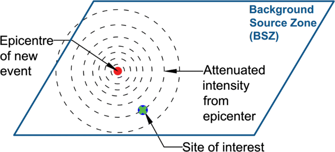

  

  Generated random event occurring within BSZs and spreading from epicentre in circles

• 8. Steps 1 to 7 are repeated for each year of synthetic catalogue until all years of synthetic catalogue are simulated.

The procedure described above assumes that maximum one earthquake event can be generated per catalogue year in a synthetic catalogue. However, Eqs. 3–4 take into account events occurring more than once in a year. This means that the occurrence of any multiple events is distributed along the whole length of a synthetic catalogue. An analysis was performed to assess the effect of this assumption on the total number of generated events and their magnitude distribution in a synthetic catalogue. The Poisson distribution probabilities of events occurring once, twice, three times and so on in a year were calculated separately to find the number of events and their associated magnitudes. The comparison of the synthetic catalogues generated using both methods showed no significant difference.

3.2 Fault source zones (FSZs)

The procedure to generate a synthetic catalogue for fault segments is slightly different from that for BSZs: instead of using the recurrence relationship, the characteristic magnitude and associated annual occurrence rate are used to generate the events, as summarised below:

• 1. A random number, $P_{rndF}$ is sampled from a uniform distribution between 0 and 1 for each year of the catalogue.

• 2. The assigned random number is compared with the annual probability of occurrence of characteristic magnitude,$P_{char}$, on that fault segment to decide if a seismic event is occurring in that year of synthetic catalogue. If $P_{rndF}$ is less than $P_{char}$ ($P_{rndF} < P_{char}$), an earthquake with characteristic magnitude $M_{char}$ is generated in that year, otherwise no seismic event occurs. Empirical relationships proposed by Wells and Coppersmith (1994) and Youngs and Coppersmith (1985) can be used to calculate $M_{char}$ and the associated recurrence intervals, respectively, by using fault geometry and slip rates.

• 3. For an earthquake event occurring on an active fault, the epicentre of each new event is assumed as random within a segment boundary. In this case, the epicentral fault line (EFL) representing the rupture length is defined parallel to the general direction of the active fault in that segment, as illustrated in Fig. 2.

  Fig. 2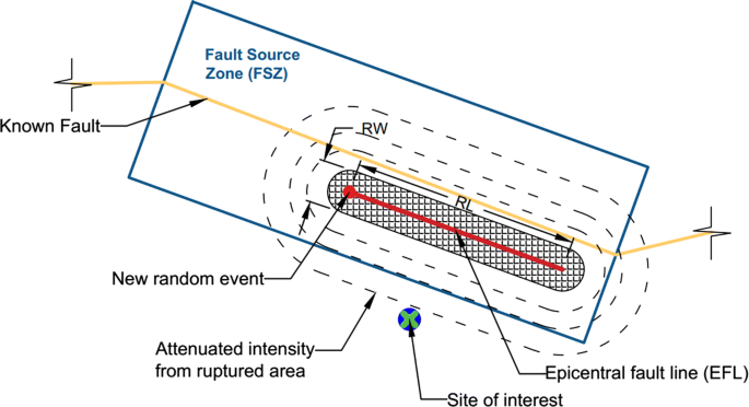

  

  Generated random event occurring at fault segment and spreading from obtained fault line

• 4. The geometry of the EFL can be estimated using magnitude relationships proposed by Wells and Coppersmith (1994):

  $$ \log \left( {SRL} \right) = - 3.22 + 0.69M_{w} $$

  (7)
  $$ \log \left( {RLD} \right) = - 2.44 + 0.59M_{w} { } $$

  (8)
  $$ \log \left( {RW} \right) = - 1.01 + 0.32M_{w} $$

  (9)

  where SRL and RLD are the surface and subsurface fault rupture length in kilometres (km), respectively; RW is the downdip fault rupture width in kilometres (km); and $M_{w}$ is the moment magnitude. The rupture length, RL, is assumed to be the maximum value of SLR and RLD. The fault segmentation model considers that a segmentation boundary exists, but it does not necessarily stop all the ruptures. The length of the rupture is calculated from Wells and Coppersmith (1994) equation and randomized with a given standard deviation. If the calculated length of the rupture is greater than the length of a segment, it will extend to another segment; hence, multi-segment rapture is considered in a way.

For a BSZ or FSZ, the total number of years of simulated earthquakes is equal to the catalogue length times the number of simulations. However, it should be noted that it is only the total number of simulated years that matters for analysis rather than the catalogue length or number of simulations individually (Musson 2012). Therefore, a catalogue with sufficient number of simulated years is necessary to capture rare events. In MC-based PSHA calculations, the period length of a synthetic catalogue is usually taken as 50 or 100 years.

3.3 Verification of background source zones

Delimitation of BSZs is not always a straightforward process, as expert opinion and subjective judgement influence this process. For example, the areal source model of the Anatolian region proposed by Erdik et al. (1999) is based on tectonic information, whereas the areal source model of Northern Europe used in the GSHAP project (Grunthal and Group 1999) follow the past seismicity pattern of the region. Moreover, seismic source models for the same study region employed by different researchers can also show variations. For instance, seismic source zones for Persian Gulf (also known as Arabian Gulf) defined by Peiris et al. (2006), Musson et al. (2006), Abdalla and Al-Homoud (2004), and Aldama-Bustos et al. (2009) all differ in size and shape.

To avoid subjectivity, an objective method for assessing BSZ is necessary. The methodology described by Musson and Winter (2012) can be used to verify source zone models by assessing them in a statistical manner via the chi-square ($X^{2}$) test. In this test, the study area under consideration is divided into equally sized grids and the number of past events from the existing earthquake catalogue is counted for each cell of the grid. If the number of events in the cell is less than a minimum threshold (determined based on cell size and number of events in the catalogue), then the cell is disregarded in the test. The next step is to assess the validity of the source model by comparing the number of real events that occurred in the past with the events predicted in the synthetic catalogue using the $X^{2}$ value:

$$ X^{2} = \mathop \sum \limits_{i = 1}^{n} \frac{{\left( {O_{i} - E_{i} } \right)^{2} }}{{E_{i} }} $$

(10)

where n is total number of cells used in the test: $O_{i}$ is the number of observed (events in the synthetic catalogue) events from MC simulation; and $E_{i}$ is the number of expected (original catalogue) events obtained from earthquake catalogue in the cell i.

The degrees of freedom ($DF$) are defined as:

$$ {\text{ DF}} = {\text{n}} - 1 $$

(11)

The $X^{2}$ and $DF$ values obtained from Eqs. 10 and 11 are checked in the $X^{2}$ distribution table to find the significance level (or probability of a larger value of $X^{2}$) of null hypothesis to be rejected. The source model can be considered to offer a viable depiction of seismicity pattern if the significance level is large enough to not reject the null hypothesis. Conventionally, a significance level of 0.05 is used as a boundary between significant and non-significant results. It should be noted that if the test is applied in a sensible way (e.g. source zones are not under-generalised) it can help to indicate a problem if the zones are too big or are in the wrong place. While Musson and Winter (2012) adopted method does not completely eliminate subjectivity, it can reduce the effects of subjectivity in the delineation of the BSZs.

3.4 Ground-motion prediction equations

Ground-motion prediction equations (GMPEs) estimate ground motion intensity (e.g. PGA, PGV or SA values at certain periods) at a site of interest and generally take the following form:

$$ \ln \left( {IM} \right) = \overline{{\ln \left( {IM} \right)}} \left( {M,R,\theta } \right) + \sigma \left( {M,R,\theta } \right) \cdot \varepsilon $$

(12)

where $\ln \left( {IM} \right)$ represents the natural logarithm of a ground motion intensity measure, which is considered to be a normally distributed random variable (Erdik 2017); $\ln \left( {IM} \right)$, $\sigma$ and $\varepsilon$ are the mean, standard deviation [consists of within-event (φ) and between-event (τ) standard deviations (SDs)] and standard normal variable, respectively; $M$ is earthquake magnitude; R is source-site distance; and $\theta$ represents the effect of style-of-faulting, soil conditions and similar parameters. The variability in $\ln \left( {IM} \right)$ is achieved by adding the product of $\sigma$ and $\varepsilon$ to the mean value, where $\varepsilon$ is a standard normal variable. To include ground motion variability in MC based PSHA within-event (φ) and between-event (τ) SDs should be considered. For each earthquake generated in the synthetic catalogue, a random number sampled from the standard normal probability distribution is multiplied by within-event (φ) SD. Another draw from the standard normal probability distribution for each site of interest is multiplied by between-event (τ) SD. Obtained values are added to the $\ln \left( {IM} \right)$ to find estimated ground motion value at each site of interest.

Different alternatives exist to calculate the value of R. Figure 3 shows the different distance metrics used in ground motion prediction equations (GMPEs) available in the literature. These include distance to hypocentre, $R_{hyp}$; the shortest distance from a site to the fault rupture, $R_{rup}$; distance to epicentre, $R_{epi}$; and the shortest horizontal distance to the point on the surface projection of the fault rupture (‘Joyner–Boore distance’) $R_{JB}$ (Joyner and Boore 1981).

Fig. 3

Fault geometry and projection on to the surface with distance metrics used in GMPEs

If the selected GMPEs were a function of $R_{hyp}$ and $R_{rup}$, integration over depth would be required in the conventional PSHA method (Bommer and Scherbaum 2008). However, in the MC-based PSHA method, there is an easy and practical way to include depth related uncertainty into hazard calculations, as depth can be entered as a distribution function during the generation of synthetic catalogues (Musson 2000).

3.5 Hazard calculation for the desired probability of exceedance level

Once synthetic catalogues for both BSZs and FSZs are generated, the probability of exceedance of ground shaking intensities (PGA, PGV or SA) can be calculated at a site of interest. For each year of a synthetic catalogue, all earthquakes occurring in that year across all source zones are used to identify the largest ground shaking intensity at the site. In other words, the worst-case scenario from all seismic sources affecting the site of interest is stored as an annual maximum outcome. This step is repeated for all simulations. The results of each simulation are combined into a single list. The probability of exceedance of ground shaking intensities can be found by sorting annual outcomes in descending order and by selecting the $N$th value in the sorted list. For the desired probability of exceedance ($PoE$), $N$ can be calculated using the following equation:

$$ N = \left( {\frac{1}{PoE} \times {\text{ Catalogue length}} \times {\text{Number of simulations}}} \right) + 1 $$

(13)

The flowchart for predicting seismic hazard at a site of interest using MC PSHA method is shown in Fig. 4.

Fig. 4

Procedure for predicting seismic hazard at a site of interest using MC-based PSHA

3.6 Near-fault directivity

Pulselike ground motions caused by near-fault forward directivity effects can have devastating consequences on structures located nearby the ruptured fault. If the rupture propagation direction and the slip direction on the fault are all aligned with the site of interest, and if the speed of the rupture propagation is similar to that of the shear wave velocity, forward rupture directivity effects can lead to the development of a single pulse of large amplitude (Somerville et al. 1997; Archuleta and Hartzell 1981; Akkar et al. 2018; Somerville 2003). It should be noted that traditional GMPEs are based on data coming from both pulselike and non-pulselike ground shaking records. Hence, they are expected to underestimate spectral acceleration for pulselike motions (Shahi and Baker 2011).

Several approaches were developed to take into account forward directivity effects on spectral acceleration values (e.g. Somerville 2003; Shahi and Baker 2011; Spudich et al. 2013). In this work, the probabilistic approach developed by Shahi and Baker (2011) is chosen for implementation, due to its effectiveness as verified through comparison with other method by Akkar et al. (2018) and its relative ease of application within MC PSHA method. In this approach, the probability of observing a pulse at ${\upalpha }$, $P\left( {\upalpha } \right)$, is calculated in accordance with Eqs. (14)–(16) using the product of a probability derived from site-to-source geometry, and the probability of observing the pulse in the orientation of interest:

$$ P\left({\upalpha } \right) = P\left( {{\upalpha }{\text{|pulse}}} \right) \times P\left( {{\text{pulse|}}r,s} \right) $$

(14)

$$ P\left( {{\upalpha }|pulse} \right) = \min \left[ {0.67;0.67 - 0.0041\left( {77.5 - {\upalpha }} \right)} \right] $$

(15)

$$ P\left( {{\text{pulse|}}r,s} \right) = \frac{1}{{1 + e^{{\left( {0.642 + 0.167r - 0.075s} \right)}} }} $$

(16)

where ${\upalpha }$ is orientation of interest measured in degrees, and r and s are site-to-source geometric parameters measured in km, as schematically shown in Fig. 5. It is important to note that Eq. (16) is valid for strike-slip faults only.

Fig. 5

Plan view explaining the parameters needed to fit in Eq. 16 for strike-slip faults

The directivity effect is experienced mostly in the fault-normal component of the ground motion, and therefore, the highest probability of observing pulse is when the orientation of interest is perpendicular to the strike (${\upalpha }$  = 90°) and the lowest when the orientation is parallel to the strike (${\upalpha }$ = 0).

Once $P\left( {\upalpha } \right)$ is calculated, occurrence of pulselike ground motion at the site of interest needs to be determined. For each year of a synthetic catalogue with an earthquake occurrence, a random number between 0 and 1 from a uniform distribution is generated. If the random number is less than $P\left( {\upalpha } \right)$ obtained from Eq. (16), a pulselike event occurs in that year, else it does not. For events that are producing pulselike ground motions, the mean period of the pulse $\mu_{{\ln T_{p} }}$ and its standard deviation $\sigma_{{\ln T_{p} }}$ are calculated as:

$$ \mu_{{\ln T_{p} }} = - 5.73 + 0.99M $$

(17)

$$ \sigma_{{\ln T_{p} }} = 0.56 $$

(18)

where $T_{p}$ is the period of the pulse; and $M$ is the earthquake magnitude.

Amplification and de-amplification factors to modify GMPEs to account for pulselike and non-pulselike behaviour are given in Shahi and Baker (2011), as well as equations of observing pulse in case of strike-normal type of faulting.

3.7 Time-dependent (renewal) analysis

The Poisson model is generally applicable to low seismicity regions or regions without major faults, as it considers earthquakes as independent events in time. Paleoseismic studies and historical seismicity observations have shown that earthquakes with similar characteristic magnitudes (same size) and similar time intervals between events tend to occur on known fault segments (Schwartz and Coppersmith 1984). It is also suggested, that for the faults with an adequate information on return period of $M_{char}$, a time-dependent model may be better at estimation of the short-term hazard assessment than a Poisson model (Akinci et al. 2009). In the renewal model, if the time interval that passed from the previous event is known for a fault segment, the conditional probability of a future characteristic event rupturing in that segment in the next $\Delta T$ years, $P_{cond} \left( {T,\Delta T} \right)$, can be calculated as follows:

$$ P_{cond} \left( {T,\Delta T} \right) = \frac{{\mathop \smallint \nolimits_{T}^{T + \Delta T} f\left( t \right)dt}}{{\mathop \smallint \nolimits_{T}^{\infty } f\left( t \right)dt}} $$

(20)

where $f\left( t \right)$ is the probability density function (PDF) for earthquake recurrence time interval; $T$ is the time passed since the last characteristic event occurred on the fault segment; and $\Delta T$ is the exposure period, taken as 50 years for typical buildings. $P_{cond} \left( {T,\Delta T} \right)$ is conditional, as it changes with time elapsed since the last earthquake. $f\left( t \right)$ can be represented with Gaussian, log-normal, Weibull, Gamma and Brownian Passage Time (BPT) models. Among these, the BPT model (which is similar to the log-normal distribution) is deemed to represent adequately the earthquake distribution (Ellsworth et al. 1999). The PDF for the BPT distribution can be calculated as:

$$ PDF\left( {t,\mu ,\alpha_{p} } \right) = \left( {\frac{\mu }{{2\pi \alpha_{p}^{2} t^{3} }}} \right)^{\frac{1}{2}} {\exp}\left( { - \frac{{\left( {t - \mu } \right)^{2} }}{{2\alpha_{p}^{2} \mu t}}} \right)^{\frac{1}{2}} { } $$

(21)

where $\mu$ is mean return period; and $\alpha_{p}$ is the aperiodicity (an equivalent to the coefficient of variation). Small values of $\alpha_{p}$ mean that the characteristic earthquakes are highly periodical. As $\alpha_{p}$ increases the conditional probability of the future characteristic event, $P_{cond} \left( {T,\Delta T} \right)$, it becomes similar to Poisson probabilities (Erdik et al. 2004). Many studies suggested a standard value of 0.5 for $\alpha_{p}$ (Cramer et al. 2000 and Erdik et al. 2004). Figure 6a, b show the PDF and $P_{cond} \left( {T,\Delta T} \right)$ for BPT model for a mean return period of $\mu$ = 300 years and exposure period of $\Delta T$ = 50 years. The figures show that the conditional probability of having a new event in the next 50 years, $P_{cond} \left( {T,50} \right)$, does not significantly increase after an approximate elapsed time of 400 years since the last event.

Fig. 6

a PDF and b conditional probability for BPT distribution with a mean return period of 300 years and α = 0.5

Once conditional probabilities for a specific exposure period are calculated from Eq. (19), they can be converted to the effective Poisson annual probabilities, $R_{eff}$ using the following equation (WGCEP94 1995):

$$ R_{eff} = - \ln \left( {1 - { }P_{cond} \left( {T,\Delta T} \right)} \right)/\Delta T $$

(21)

3.8 Uncertainty in PSHA

There are two types of uncertainties that exist in earthquake hazard analysis: aleatory and epistemic uncertainties. Aleatory uncertainty represents the natural randomness in a process, while epistemic uncertainty is the lack of knowledge introduced in a model that tries to represent an actual behaviour. The aleatory variability arises from the randomness of the earthquake generation process, and is usually taken into account with a probability distribution. Epistemic uncertainty on the other hand arises from the lack of knowledge about the true single value of a variable. Parameters that define a probability density function (e.g. mean and standard deviation of a normal distribution) have in fact one true value, which we don't know.

In PSHA analysis, the standard deviation of GMPEs can be used to deal with aleatory uncertainty. Epistemic uncertainty can be addressed with a logic tree, in which weights are applied to the branches to reflect confidence in given options (Bommer et al. 2005; Scherbaum et al. 2005). Figure 7 shows an example of a logic tree that utilises several GMPEs.

Fig. 7

An example of the logic tree for ground motion prediction equations

It should be noted that logic trees can be used to include different hypotheses in PSHA. For example, they are often used for altering recurrence rates of faults, geometry of seismic source zones, and characteristic magnitudes. The use of a MC-based approach in PSHA can reduce the number of parameters employed in the logic trees because many of the mentioned parameters are already randomized during the synthetic catalogue generation process.

The previous sections provided an overview of the components of the utilised MC-based PSHA. To demonstrate the method, the following section uses a case study region to verify the effectiveness of the developed computational tool.

4 The case study: Marmara region, Turkey

To demonstrate developed PSHA tool, Marmara region (Turkey) is selected as a case study area. This region is located in one of the most seismically active zones in the world. It houses one-third of Turkey’s population and is a major industrial hub for the country. Both 1999 Kocaeli and Duzce earthquakes occurred in this region and caused enormous economic losses, extensive structural damage to structures and a high fatality rate. An event of similar magnitude to these earthquakes is expected to hit Istanbul in the near future. For example, Murru et al. (2016) predict the probability of having an earthquake with M ≥ 7.0 in Istanbul to be at around 50% in the next 30 years. This earthquake is expected to be more severe and damaging compared to those of Kocaeli and Duzce as Istanbul is very densely populated and a large proportion of structures are substandard (Bal et al. 2008).

4.1 Tectonic setting of Marmara region

The North Anatolian Fault (NAF) lies across northern Turkey (see NAFZ in Fig. 8) for more than 1,500 km starting from Karliova in the east and extending to the Gulf of Saros in the west. The NAF is a right-lateral strike-slip transform fault system, along which the Anatolian plate is pushed westwards by the collision between the Arabian and Eurasian plates. The western portion of the NAF zone dominates the tectonic regime of the Marmara Sea area: the NAF zone continues as a single fault line east of 31.5°E, whereas to the west it splays into a complex fault system that has created multiple strong seismic events over the last century (see Fig. 9). Three main branches can be identified including the northern NAF (NNAF), central NAF (CNAF) and southern NAF (SNAF) branches. The NNAF is the most active branch with slip rates of 14–24 mm/year, while CNAF and SNAF branches move only 2–8 mm/year (Murru et al. 2016). The NNAF branch enters the eastern part of the Marmara Sea at the Gulf of Izmit, then bends to the north shelf of the sea, and eventually joins NE-SW striking the Ganos fault onshore. Here, the branch extends until entering the Aegean Sea through the Gulf of Saros (Kurt et al. 2000; McNeill et al. 2004). Unlike NNAF, the CNAF and SNAF branches span to the south of the Marmara Sea. CNAF goes underwater through the Marmara Sea by entering at Gemlik Bay and emerging on land briefly. At 27.8°E, the CNAF branch turns toward south-west to join the faults in the North Aegean region.

Fig. 8

Tectonic setting of Turkey. EAFZ—East Anatolian Fault Zone, NAFZ—North Anatolian Fault Zone, NEAFZ—North East Anatolian Fault Zone, DSFZ—Dead Sea Fault Zone (Faults data is taken from https://www.efehr.org)

Fig. 9

Faults system in Marmara region with epicentral location of major earthquakes occurred in twentieth century (Faults data is taken from https://www.efehr.org)

The high-resolution bathymetric survey in the Marmara Sea provided indication of a continuous strike-slip faulting system going through the northern part of the Marmara Sea. It also provided a better understanding of the behaviour of the faults with seismic gap and linked the 1999 Kocaeli earthquake fault with the 1912 Sarkoy-Murefte earthquake fault (Erdik et al. 2004).

4.2 Seismicity of the Marmara Region

As the capital of both Byzantine and Ottoman empires, Istanbul has been populated for millennia and therefore there is evidence of historical seismicity. Furthermore, the effect of past earthquakes can be tracked by observing damage and repairs on historical structures, which can serve as an indicator of previous seismic events. During the twentieth century, Marmara has experienced relatively high seismicity with several M > 7.0 earthquakes occurring on the NAF. Table 1 summarises the magnitudes and dates of major historical events of $M_{s} \ge 7$ since 1500 CE. The table shows a recent series of strong earthquakes, which ruptured along the NAF, starting further east with the M_w = 7.8 Erzincan earthquake (1939) and propagating towards the west into the Marmara region. The Kocaeli (1999) and Duzce (1999) earthquakes were the last events associated with the westward propagation at the NAF (Alpar and Yaltirak 2002).

Table 1 List of $M_{s} \ge 7$ earthquakes in Marmara Region from 1500 CE to present.

It is well-established that there is a potential seismic gap in the region of the Marmara Sea to the south of Istanbul (Bohnhoff et al. 2013). The fault in this area has not ruptured for at least 200 years, although there is evidence of large historical events taking place around this seismic gap (e.g. the 1766 Istanbul earthquake). The length of the gap is around 150 km and it has a potential of generating an earthquake with M > 7.0 similar to previous earthquakes at this location (Hubert-Ferrari et al. 2000). An earthquake of that magnitude and proximity to Istanbul would have devastating consequences and, therefore, it is crucial to understand the potential hazard associated with this seismic gap to develop appropriate seismic mitigation and prevention strategies.

4.3 Homogenisation, clustering and completeness of the earthquake catalogue

In this study, the instrumental earthquake catalogue developed by Turkey’s Disaster and Emergency Management Presidency (AFAD) (https://deprem.afad.gov.tr/) is utilised for the case study area. This catalogue consists of seismic events with $M$ ≥ 4 that occurred between 1900 and 2018 in the Marmara region. Most of the earthquake data are reported in terms of surface-wave magnitude scale, $M_{s}$, for the first half of twentieth century, while more magnitude scales are used for more recent events. Historical events that occurred in the region are included in the catalogue using data from Ambraseys and Jackson (2000). A catalogue homogenisation was necessary to convert $M_{s}$, $M_{L}$ and $m_{b}$ magnitude scales into moment magnitude, $M_{w}$, and this was done using conversion equations specifically developed for Turkey by Kadirioğlu and Kartal (2016).

After homogenisation, the data need to be declustered for the removal of dependent events (fore- and after-shocks).

Table 2 lists the number of mainshocks and dependent events according to each method in the refined earthquake catalogue. It can be seen from this table that Gardner and Knopoff (1974) approach removes 50.88% of events in catalogue due to the fact that the time and space windows are larger compared to those obtained with the modified Knopoff (2000) method. Consequently, the former method leads to smaller earthquake occurrence rates. Therefore, this work uses the modified Knopoff (2000) method for subsequent analysis to stay on the conservative side.

Table 2 Summary of dependent events removed for final catalogue using different algorithms

After homogenization and declustering, the number of event below $M_{w}$ < 4.1 was found to be considerably low. Therefore, for the catalogue obtained for the study area the minimum completeness magnitude was set to $M_{w}$ = 4.1. Figure 10a–d shows the results of completeness analysis performed for the case study area following procedure described by Aldama-Bustos (2009). In this figure, black dashed vertical lines show the start of the completeness period, and red horizontal lines show the estimated mean occurrence rate for the completeness period. The results in Fig. 10a–d indicate that the declustered catalogue may be regarded as being complete above $M_{w}$ = 4.1 from 1963 onwards, $M_{w}$ = 5.0 from 1900 onwards, $M_{w}$ = 6.0 from 1840 and $M_{w}$ = 7.0 from 1660. Levels of completeness are adopted for other magnitudes and periods following the chosen algorithm.

Fig. 10

Instrumental earthquake catalogue completeness analysis showing mean annual occurrence rate of events for a M_w ≥ 4.2, b M_w ≥ 5.0, c M_w ≥ 6.0, and d M_w ≥ 7.0

It should be noted that catalogue homogenization, completeness analysis and declustering presented are incorporated into the code and automated. Nevertheless, user intervention and judgement are always required for a rigorous treatment of the catalogue issues such as determination of completeness date.

4.4 Source zones

The seismicity of the Marmara region is represented with the fault segmentation and background seismicity model. Table 3 provides information on the seismicity parameters for each of the BSZs used in this study (such as a and b parameters of the Gutenberg–Richter relationship, and the minimum and maximum earthquake magnitudes$, M_{min}$ and $M_{max}$, associated with each source zone). $M_{max}$ is based on the maximum observed magnitude in the source zone from historical data. BSZs are delineated by the user, but by utilising $X^{2}$ test validation zones are altered until satisfactory result is obtained. Figure 11 shows the derived BSZs for the Marmara region. A source zone number is assigned to each BSZ, as shown in the figure. The maximum likelihood estimation procedure developed by Weichert (1980) is integrated into the code to estimate the b parameter of the Gutenberg-Richter relationship by accounting for different years of completeness period for each magnitude range. The location of synthetic earthquakes within BSZs and FSZs are randomized with a uniform distribution to treat aleatory uncertainty. Also, the code developed allows the user to treat earthquakes in BSZs as points or ruptures. For the case study example, earthquakes occurring within BSZs are assumed as point sources for a computational efficiency. In general, this does not make a big difference, except for a few zones where the $M_{max}$ is high.

Table 3 Seismicity parameters for BSZs used in this study

Fig. 11

source model used in the PSHA presented in this study. Zone numbers and corresponding parameters are listed in Table 3

Background

The validity of the source model is verified via the $X^{2}$ test, as explained in Sect. 3.3. Figure 12a shows the locations of the instrumental historical earthquake events in the Marmara region, whereas Fig. 12b illustrates the earthquake locations from one of the synthetic catalogues. By counting and comparing the cell counts in each BSZ from instrumental and synthetic catalogues, $X^{2}$ values are calculated using Eq. (10). Cells with less than 15 events are excluded from the analysis (e.g. brown coloured cell in Fig. 12a). The process is repeated for each of the 1000 simulated catalogues and the $X^{2}$ statistic is calculated to be 5.24, thus proving the hypothesis that there was no significant difference between the synthetic catalogue and the recorded events.

Fig. 12

Distribution of a historical events and b events in one of the simulated catalogues occurred in the Marmara region

Aggregate testing (Musson and Winter 2012) can be utilised to compare activity rates obtained from original and synthetic catalogues for each BSZ. Mean magnitude and total number of events are then calculated for each synthetic catalogue generated in the MC process. The data obtained from all synthetic catalogues are then grouped into magnitude-total number of seismic event bins. The number of catalogues coinciding to each mean magnitude and number of event ranges result in a surface plot, where the peak value shows the most repeating value for the number of event vs mean magnitude. The pair of mean magnitude and number of events calculated from the original catalogue provides a point for a comparison with this distribution. If the point is relatively close to the peak of distribution, the model can be considered to adequately represent the activity rate of the background zone. As an example, Fig. 13 shows the result of analysis for one of the BSZ (# 3) showing 100 years’ seismicity. One can see from this figure that the synthetic catalogues result in a modal value of 63 events and mean magnitude of 4.63, whereas historical outcome produces 63 events with a mean magnitude of 4.53. Relatively close values imply that the activity rates assigned to the considered BSZ are consistent with the past earthquake data.

Fig. 13

Frequency plot showing 100 years’ seismicity generated for one of a BSZs produces by the model. The arrow indicates the point of values obtained from original catalogue in that BSZ

The segmentation model proposed by Erdik et al. (2004) (see Fig. 14), which assumes that the total accumulated energy along well-defined fault segments of the region is released through characteristic earthquakes is adopted for this region. The developed code is capable of calculating return period from slip rates and $M_{char}$ for each fault segment if available, which are computed through empirical relations (Wells and Coppersmith 1994), but for the case study area $M_{char}$ values and Poissonian rates were adopted from Erdik et al. (2004) with a manual input. The basic parameters associated with the faults segments are shown in Table 4. The table also lists calculated annual rates of time-dependent method described in the Sect. 3.7.

Fig. 14

The fault segmentation model proposed by Erdik et al. (2004) for the Marmara region

Table 4 Poisson and time-dependent annual rates for the fault segmentation model

To take into account aleatory uncertainty, the mean of the $M_{char}$ value is randomized with a uniform distribution by sampling value between − 0.25 and 0.25 and adding it to the mean of the $M_{char}$.

4.5 Ground motion prediction equations (GMPEs) used for the study area

In this study, the GMPEs proposed by Akkar et al. (2014) and Boore et al. (2014) are employed to calculate the earthquake hazard in terms PGA and SAs. To treat epistemic uncertainty, a logic tree is used, allocating weights of 0.7 and 0.3 to each branch for the GMPEs of Akkar et al. (2014) and Boore et al. (2014), respectively. Higher weight is given to Akkar et al. (2014) equation because such model contains a large proportion of recordings from Turkey. Moreover, in this GMPE, the majority of recordings for strike-slip mechanism events with M > 7 are taken from earthquakes which occurred in the Marmara region. The GMPE proposed by Boore et al. (2014) is one of the few GMPEs that satisfy the requirements for use in PSHA specified by Bommer et al. (2010). In this GMPE, inter-event and intra-event variabilities are calculated for different magnitude ranges based on period, distance or soil conditions. It also employs a correction factor for various seismic active regions around the world including Turkey.

5 Results

The procedures presented in this paper are implemented for the region using a Matlab code. Hazard maps considering these models for PGA and SA at T = 0.2 s and T = 1.0 s for a Probability of Exceedance (POE) of 10% (i.e. a return period of 475 years) and 2% in 50 years (return periods of 2475 years) are generated for the region. Design earthquakes are also derived for a specific location in the Marmara region.

5.1 Hazard maps

Figures 15 and 16 show PGA hazard maps derived using Poisson and time-dependent models, respectively. Both maps are for a return period of 475 years. It is shown that there is a noticeable difference between the PGA values obtained using the Poisson and time-dependent models, even though nearly two decades have passed since the 1999 Kocaeli earthquake. The annual rates calculated for the time-dependent model for the fault segments (1 to 4 from Table 4) relatively close to Izmit area are about a third of those used in the Poisson model. As a result of this, lower hazard levels are obtained in the time-dependent model for the eastern part of the Marmara region. On the other hand, hazard levels are slightly higher in the western part of the Marmara region, due to the fact that no fault ruptures occurred since the eighteenth century. Both models predict PGA levels between 0.30 g and 0.45 g for a 475 year return period for Istanbul’s metropolitan area, which creates a high risk for this densely populated city. The hazard level for Istanbul area is considerably higher in the time-dependent model than that obtained using the Poisson model. This is because some unruptured NAF segments (seismic gap) in the Marmara Sea have a higher probability of generating characteristic events with M > 7. In both figures, the highest PGAs are predicted in the southern part of Istanbul, where the Bosporus meets with the Marmara Sea. The expected seismic hazard gradually reduces towards the north of the city. Predicted hazard levels for PGA corresponding to a return period of 2475 years are given in Figs. 17 and 18 using the Poisson and time-dependent models, respectively. It can be seen that the maximum PGA levels for rock conditions using the Poisson and time-dependent models are as high as 0.80 g for 475 years return period and 1.36 g for 2475 years return period across the case study area.

Fig. 15

Seismic hazard map of Marmara region for PGA (g) considering 10% probability of exceedance in 50 years (the Poisson model)

Fig. 16

Seismic hazard map of Marmara region for PGA (g) considering 10% probability of exceedance in 50 years (Time-dependent model)

Fig. 17

Seismic hazard map of Marmara region for PGA (g) considering 2% probability of exceedance in 50 years (the Poisson model)

Fig. 18

Seismic hazard map of Marmara region for PGA (g) considering 2% probability of exceedance in 50 years (Time-dependent model)

Hazard maps for SA at T = 0.2 s with return periods of 475 and 2475 years for the Poisson model are compared in Figs. 19 and 20, respectively. The maximum values of SA at T = 0.2 s is found to be as high as 1.67 g and 2.61 g for 475 and 2475 years of return periods, respectively. Figures 21 and 22 show the hazard maps for SA at T = 1.0 s with return periods of 475 and 2475 years, respectively, calculated using the Poisson model. In this case, the maximum values of SA at T = 1.0 s are found to be as high as 0.50 g and 0.92 g for 475 and 2475 years of return periods, respectively.

Fig. 19

Seismic hazard map of Marmara region for SA (g) T = 0.2 s considering 10% probability of exceedance in 50 years (the Poisson model)

Fig. 20

Seismic hazard map of Marmara region for SA (g) T = 0.2 s considering 2% probability of exceedance in 50 years (the Poisson model)

Fig. 21

Seismic hazard map of Marmara region for SA (g) T = 1.0 s considering 10% probability of exceedance in 50 years (the Poisson model)

Fig. 22

Seismic hazard map of Marmara region for SA (g) T = 1.0 s considering 2% probability of exceedance in 50 years (the Poisson model)

Seismic hazard maps with and without consideration of near-field effect are also compared in Figs. 23 and 24, respectively, for T = 2.0 s and POE 2% in 50 years. It is found that near-field directivity increases SA values around active faults (e.g. Izmit area) by approximately SA of 10–20%.

Fig. 23

Seismic hazard map of Marmara region for SA (g) T = 2.0 s considering 2% probability of exceedance in 50 years employing the Poisson model including near-field directivity effects

Fig. 24

Seismic hazard map of Marmara region for SA (g) T = 2.0 s considering 2% probability of exceedance in 50 years (the Poisson model)

The results in Table 5 indicate that the directivity effect can have influence the predicted PSHA results by up to 20%, as can be observed for Izmit. For the areas at some distance from the fault, the directivity effect has no effect (e.g. Bursa). Particularly, this may have impact on the structures with long periods.

Table 5 Comparison of SA(2 s) results for 475 years return period with and without directivity effect for major cities of Marmara region

The results of the study were validated via comparison with the other PSHA studies for the study area, mainly to confirm they are not an outlier. This also provides some indication how realistic the results are in the presented study, given that a different approach has been used for PSHA. The hazard maps are compared with those developed by the recent SHARE project (Woessner et al. 2015), by Kalkan et al. (2008), and by Turkey’s AFAD (2018). It should be noted that AFAD’s map is included in the latest version of the Turkish Earthquake Design code Sesetyan et al. (2018). Table 6 compares the estimated PGA levels for a return period of 475 years obtained for major cities in the Marmara region. The differences between PGA (g) values obtained from this study and SHARE project (EFEHR 2018) is also shown as a colour map in Fig. 25. It can be concluded that, despite some differences, there is a good overall agreement between the results of this study with those reported in SHARE project for a return period of 475 years.

Table 6 Comparison of PGA results with those from other studies for 475 years return period, major cities of Marmara region

Fig. 25

Comparison of results of this study with SHARE project, shown as difference in PGA values for 475 years return period

5.2 Identification of design earthquakes

One of the main uses of the proposed MC-based PSHA tool is that it can be used to identify design earthquakes at sites of interest. To achieve this, all earthquake events that produce the target hazard value according to a probability of exceedance (with a plus/minus tolerance level) are extracted from the synthetic catalogues. Then, a 3D surface graph is created for a range of magnitude and distance combinations, and with a third dimension showing the number of occurrences of events. The peaks in the graph identify potential design earthquakes in terms of magnitude and distance. As an example, for a location in central Istanbul, the PGA value of 0.35 g with a return period of 475 years is assumed. Figure 26 shows that this PGA value at the site is most likely to be produced by a modal earthquake of M_w = 7.25 at a distance of 10 km. This information can be used as input data for the assessment of secondary hazards (e.g. landslides or liquefaction), or to help select appropriate time-history earthquake records for earthquake structural analysis.

Fig. 26

Design earthquakes in terms of distance and magnitude for a design PGA = 0.35 g (± 0.01 g) for a location in Istanbul, with POE of 10% in 50 years and calculated using a Poisson model

The framework as a whole can be applicable to regions where fault data exist. On the other hand, in the areas of low seismicity, where there are no active faults, BSZs procedure alone described in the paper can be still used to perform PSHA.

6 Conclusions

This article proposes a practical MC-based PSHA tool for which synthetic earthquake catalogues are created by using readily available information on the seismo-tectonic structure, seismicity and geology of a region. Fault segmentation and background seismicity models are used to represent seismicity. The proposed background zones are verified via the $X^{2}$ test with associated seismicity parameters to check if the seismic zones can replicate the (instrumental) past seismicity. Both Poisson and time-dependent (renewal) seismic hazard models are adopted and near-field rupture directivity effects are accounted for in the model. To demonstrate the proposed computational tool, the Marmara region in Turkey is used as a case study area. The results show that the generated hazard maps compare well with results from recent PSHA studies (AFAD and SHARE). The hazard results are used to identify the design earthquake for central Istanbul. The developed tool will be incorporated into a multi-hazard seismic risk assessment framework, which will provide decision-makers, government, insurance industry and practitioners with practical risk evaluation methodologies to reduce earthquake-related losses and promote sustainable development of earthquake prone areas in the world. By using the proposed tool, designers can assess the expected seismic hazard by taking into account the time-dependent renewal characteristics of the seismic sources. Moreover, the likely impact of near-field directivity effects on the probable seismic actions can be considered directly. The decision makers can utilize the proposed tool for developing strategies by assessing the risk with a greater level of resolution. They can effectively differentiate in between the risks associated with different subregions within their area of interest, by modelling the directivity effects associated with the probable rupture scenarios.

References

Abdalla JA, Al-Homoud AS (2004) Seismic hazard assessment of United Arab Emirates and its surroundings. J Earthq Eng 8:817–837
AFAD (2018) Republic of Turkey prime ministry disaster and emergency management authority. On internet at https://tdth.afad.gov.tr/. Accessed 27 Nov 2018.
Akinci A, Galadini F, Pantosti D, Petersen M, Malagnini L, Perkins D (2009) Effect of time dependence on probabilistic seismic-hazard maps and deaggregation for the Central Apennines. Italy. Bull Seismol Soc Am 99(2A):585–610
Akkar S, Cheng Y (2015) Application of a Monte-Carlo simulation approach for the probabilistic assessment of seismic hazard for geographically distributed portfolio. Earthq Eng Struct Dyn 45(4):525–541
Akkar S, Sandikkaya M, Bommer J (2014) Empirical ground- motion models for point- and extended- source crustal earthquake scenarios in Europe and the Middle East. Off Publ Eur Assoc Earthq Eng 12:359–387
Akkar S, Moghimi S, Arici Y (2018) A study on major seismological and fault-site parameters affecting near-fault directivity ground-motion demands for strike-slip faulting for their possible inclusion in seismic design codes. Soil Dyn Earthq Eng 104:88–105
Aldama-Bustos G (2009) An exploratory study of parameter sensitivity, representation of results and extensions of PSHA: case study-United Arab Emirates. PhD Dissertation, Imperial College London
Aldama-Bustos G, Bommer J, Fenton C, Stafford P (2009) Probabilistic seismic hazard analysis for rock sites in the cities of Abu Dhabi, Dubai and Ra's Al Khaymah, United Arab Emirates. Georisk 3:1–29
Alpar B, Yaltirak C (2002) Characteristic features of the North Anatolian Fault in the eastern Marmara region and its tectonic evolution. Mar Geol 190:329–350
Ambraseys NN, Jackson J (2000) Seismicity of the Sea of Marmara (Turkey) since 1500. Geophys J Int 141(3):F1–F6
Archuleta RJ, Hartzell SH (1981) Effects of fault finiteness on near-source ground motion. Bull Seismol Soc Am 71:939–957
Bal IE, Crowley H, Pinho R, Gülay FG (2008) Detailed assessment of structural characteristics of Turkish RC building stock for loss assessment models. Soil Dyn Earthq Eng 28:914–932
Bohnhoff M, Bulut F, Dresen G, Malin PE, Eken T, Aktar M (2013) An earthquake gap south of Istanbul. Nat Commun 4:1999
Bommer JJ, Spence R, Pinho R (2006) Earthquake loss estimation models: time to open the black boxes. In: First European conference on earthquake engineering and seismology, Geneva 3–8 September, 2006.
Bommer JJ, Scherbaum F (2008) The use and misuse of logic trees in probabilistic seismic hazard analysis. Earthq Spectra 24:997–1009
Bommer JJ, Scherbaum F, Bungum H, Cotton F, Sabetta F, Abrahamson NA (2005) On the use of logic trees for ground-motion prediction equations in seismic-hazard analysis. Bull Seismol Soc Am 95:377–389
Bommer JJ, Douglas J, Scherbaum F, Cotton F, Bungum H, FäH D (2010) On the selection of ground-motion prediction equations for seismic hazard analysis. Seismol Res Lett 81:783–793
Boore DM, Stewart JP, Seyhan E, Atkinson GM (2014) NGA-West2 equations for predicting PGA, PGV, and 5% damped PSA for shallow crustal earthquakes. Earthq Spectra 30:1057–1085
Chiou BS, Youngs RR (2014) Update of the Chiou and Youngs NGA model for the average horizontal component of peak ground motion and response spectra. Earthq Spectra 30:1117–1153
Console R, Falcone G, Karakostas V, Murru M, Papadimitriou E, Rhoades D (2013) Renewal models and coseismic stress transfer in the Corinth Gulf, Greece, fault system. J Geophys Res Solid Earth 118:3655–3673
Cornell CA (1968) Engineering seismic risk analysis. Bull Seismol Soc Am 58:1583–1606
Cramer CH, Petersen MD, Cao T, Toppozada TR, Reichle M (2000) A time-dependent probabilistic seismic-hazard model for California. Bull Seismol Soc Am 90:1–21
Crowley H, Bommer JJ (2006) Modelling seismic hazard in earthquake loss models with spatially distributed exposure. Off Publ Eur Assoc Earthq Eng 4:275–275
EFEHR (2018) European facilities for earthquake hazard and risk. On internet at https://www.efehr.org/. Accessed 21 Sept 2018
Ellsworth WL, Matthews MV, Nadeau RM, Nishenko SP, Reasenberg PA, Simpson RW (1999) A physically-based earthquake recurrence model for estimation of long-term earthquake probabilities. US Geol Surv Open File Rept 99(522):23
Erdik M (2017) Earthquake risk assessment. Bull Earthq Eng 15:5055–5092
Erdik M, Biro YA, Onur T, Sesetyan K, Birgoren G (1999) Assessment of earthquake hazard in Turkey and neighboring. Ann Geophys 42:1125–1138
Erdik M, Demircioglu M, Sesetyan K, Durukal E, Siyahi B (2004) Earthquake hazard in Marmara Region, Turkey. Soil Dyn Earthq Eng 24:605–631
Gardner J, Knopoff L (1974) Is the sequence of earthquakes in Southern California, with aftershocks removed, Poissonian? Bull Seismol Soc Am 64:1363–1367
Grünthal G, GSHAP Region 3 Working Group (1999) Seismic hazard assessment for Central, North and Northwest Europe: GSHAP Region 3. Ann Geophys 42:999–1011
Hubert-Ferrari A, Barka A, Jacques E, Nalbant SS, Meyer B, Armijo R, Tapponnier P, King GC (2000) Seismic hazard in the Marmara Sea region following the 17 August 1999 Izmit earthquake. Nature 404:269
Joyner WB, Boore DM (1981) Peak horizontal acceleration and velocity from strong-motion records including records from the 1979 Imperial Valley, California, earthquake. Bull Seismol Soc Am 71:2011–2038
Kadirioğlu FT, Kartal RF (2016) The new empirical magnitude conversion relations using an improved earthquake catalogue for Turkey and its near vicinity (1900–2012). Turk J Earth Sci 25:300–310
Kalkan E, Gülkan P, Öztürk NY, Çelebi M (2008) Seismic hazard in the istanbul metropolitan area: a preliminary re-evaluation. J Earthq Eng 12:151–164
Kijko A (2004) Estimation of the maximum earthquake magnitude, Mmax. Pure Appl Geophys 161:1655–1681
Knopoff L (2000) The magnitude distribution of declustered earthquakes in Southern California. Proc Natl Acad Sci 97:11880–11884
Krinitzsky EL (2003) How to combine deterministic and probabilistic methods for assessing earthquake hazards. Eng Geol 70:157–163
Kurt H, Demirbaǧ E, Kuşçu İ (2000) Active submarine tectonism and formation of the Gulf of Saros, Northeast Aegean Sea, inferred from multi-channel seismic reflection data. Mar Geol 165:13–26
Malhotra PK (1999) Response of buildings to near-field pulse-like ground motions. Earthq Eng Struct Dyn 28:1309–1326
Mcguire RK (1995) Probabilistic seismic hazard analysis and design earthquakes: closing the loop. Bull Seismol Soc Am 85:1275–1284
Mcneill LC, Mille A, Minshull TA, Bull JM, Kenyon NH, Ivanov M (2004) Extension of the North Anatolian fault into the North Aegean trough: evidence for transtension, strain partitioning, and analogues for Sea of Marmara basin models. Tectonics. https://doi.org/10.1029/2002TC001490
Murru M, Akinci A, Falcone G, Pucci S, Console R, Parsons T (2016) M≥ 7 earthquake rupture forecast and time-dependent probability for the Sea of Marmara region, Turkey. J Geophys Res Solid Earth 121:2679–2707
Musson RMW (1999) Determination of design earthquakes in seismic hazard analysis through Monte-Carlo simulation. J Earthq Eng 3:463–474
Musson RMW (2000) The use of Monte Carlo simulations for seismic hazard assessment in the UK. Ann Geofis 43:1–9
Musson RMW (2012) PSHA validated by quasi observational means. Seismol Res Lett 83:130–134
Musson RMW, Northmore K, Sargeant S, Phillips E, Boon D, Long D, Mccue K, Ambraseys NN (2006) The geology and geophysics of the United Arab Emirates. Geol Hazards 4:237
Musson RMW, Winter P (2012) Objective assessment of source models for seismic hazard studies: with a worked example from UK data. Bull Earthq Eng 10:367–378
Peiris N, Free M, Lubkowski Z, Hussein A (2006) Seismic hazard and seismic design requirements for the Arabian Gulf region. In: First European conference on earthquake engineering and seismology, Geneva 3–8 September, 2006.
Reasenberg P (1985) Second-order moment of central California seismicity, 1969–1982. J Geophys Res Solid Earth 90:5479–5495
Scherbaum F, Bommer JJ, Bungum H, Cotton F, Abrahamson NA (2005) Composite ground-motion models and logic trees: methodology, sensitivities, and uncertainties. Bull Seismol Soc Am 95:1575–1593
Schwartz DP, Coppersmith KJ (1984) Fault behavior and characteristic earthquakes—examples from the Wasatch and San-Andreas fault zones. J Geophys Res 89:5681–5698
Sesetyan K, Demircioglu MB, Duman TY, Çan T, Tekin S, Azak TE, Fercan ÖZ (2018) A probabilistic seismic hazard assessment for the Turkish territory—part I: the area source model. Bull Earthq Eng 16:3367–3397
Shahi SK, Baker JW (2011) An empirically calibrated framework for including the effects of near-fault directivity in probabilistic seismic hazard analysis. Bull Seismol Soc Am 101:742–755
Silva V, Crowley H, Varum H, Pinho R (2015) Seismic risk assessment for mainland Portugal. Bull Earthq Eng 13:429–457
Somerville PG (2003) Magnitude scaling of the near fault rupture directivity pulse. Phys Earth Planet Inter 137:201–212
Somerville PG, Smith NF, Graves RW, Abrahamson NA (1997) Modification of empirical strong ground motion attenuation relations to include the amplitude and duration effects of rupture directivity. Seismol Res Lett 68:199–222
Spudich P, Bayless JR, Baker JW, Chiou BS, Rowshandel B, Shahi SK, Somerville PG (2013) Final report of the NGA-West2 directivity working group. Pacific Earthquake Engineering Research Center, PEER 2013/09. University of California, Berkeley, 2013.
Stepp J (1972) Analysis of completeness of the earthquake sample in the Puget Sound area and its effect on statistical estimates of earthquake hazard. Proceedings of the international conference on microzonation for safer construction: research and application, Seattle, USA 2:897–909
Weichert DH (1980) Estimation of the earthquake recurrence parameters for unequal observation periods for different magnitudes. Bull Seismol Soc Am 70:1337–1346
Wells DL, Coppersmith KJ (1994) New empirical relationships among magnitude, rupture length, rupture width, rupture area, and surface displacement. Bull Seismol Soc Am 84:974–1002
WGCEP94, (1995) Seismic hazards in Southern California: probable earthquakes, 1994 to 2024. Bull Seismol Seismol Soc Am 85:379–439
Woessner J, Laurentiu D, Giardini D, Crowley H, Cotton F, Grünthal G, Valensise G, Arvidsson R, Basili R, Demircioglu MB, Hiemer S, Meletti C, Musson RMW, Rovida AN, Sesetyan K, Stucchi M, Consortium TS (2015) The 2013 European Seismic Hazard Model: key components and results. Bull Earthq Eng 13:3553–3596
Youngs RR, Coppersmith KJ (1985) Implications of fault slip rates and earthquake recurrence models to probabilistic seismic hazard estimates. Bull Seismol Soc Am 75:939–964
Acknowledgements
The research leading to these results has received funding from the RCUK-TUBITAK Research Partnerships Newton Fund Awards under grant agreement EP/P010016/1. The authors also acknowledge the support provided by the British Council Newton Fund through project No. 216425146. We are also grateful to Prof. Yasin Fahjan from Gebze Technical University for providing insightful and constructive comments on the manuscript.
Author information
Authors and Affiliations
Corresponding author
Additional information
Publisher's Note
Springer Nature remains neutral with regard to jurisdictional claims in published maps and institutional affiliations.
Rights and permissions
Open Access This article is licensed under a Creative Commons Attribution 4.0 International License, which permits use, sharing, adaptation, distribution and reproduction in any medium or format, as long as you give appropriate credit to the original author(s) and the source, provide a link to the Creative Commons licence, and indicate if changes were made. The images or other third party material in this article are included in the article's Creative Commons licence, unless indicated otherwise in a credit line to the material. If material is not included in the article's Creative Commons licence and your intended use is not permitted by statutory regulation or exceeds the permitted use, you will need to obtain permission directly from the copyright holder. To view a copy of this licence, visit http://creativecommons.org/licenses/by/4.0/.
About this article
Cite this article
Sianko, I., Ozdemir, Z., Khoshkholghi, S. et al. A practical probabilistic earthquake hazard analysis tool: case study Marmara region. Bull Earthquake Eng 18, 2523–2555 (2020). https://doi.org/10.1007/s10518-020-00793-4
Received:
Accepted:
Published:
Issue Date:
DOI: https://doi.org/10.1007/s10518-020-00793-4