Analytical and numerical seismic assessment of heritage masonry towers

Abstract

The new Italian building code, published in 2018 [MIT in NTC 2018: D.M. del Ministero delle Infrastrutture e dei trasporti del 17/01/2018. Aggiornamento delle Norme Tecniche per le Costruzioni (in Italian), 2018], explicitly refers to the Italian “Guidelines for the assessment and mitigation of the seismic risk of the cultural heritage” [PCM in DPCM 2011: Direttiva del Presidente del Consiglio dei Ministri per valutazione e riduzione del rischio sismico del patrimonio culturale con riferimento alle norme tecniche per le costruzioni, G.U. n. 47 (in Italian), 2011] as a reliable source of guidance that can be employed for the vulnerability assessment of heritage buildings under seismic loads. According to these guidelines, three evaluation levels are introduced to analyse and assess the seismic capacity of historic masonry structures, namely: (1) simplified global static analyses; (2) kinematic analyses based on local collapse mechanisms, (3) detailed global analyses. Because of the complexity and the large variety of existing masonry typologies, which makes it particularly problematic to adopt a unique procedure for all existing structures, the guidelines provide different simplified analysis approaches for different structural configurations, e.g. churches, palaces, towers. Among the existing typologies of masonry structures there considered, this work aims to deepen validity, effectiveness and scope of application of the Italian guidelines with respect to heritage masonry towers. The three evaluation levels proposed by the guidelines are here compared by discussing the seismic risk assessment of a representative masonry tower: the Cugnanesi tower located in San Gimignano (Italy). The results show that global failure modes due to local stress concentrations cannot be identified if only simplified static and kinematic analyses are performed. Detailed global analyses are in fact generally needed for a reliable prediction of the seismic performance of such structures.

1 Introduction

The seismic performance assessment of monumental buildings plays a key role in the maintenance and safety of the architectural heritage, allowing to design and programme appropriate preservation strategies. Recent seismic events in Central Italy (Abruzzo, L’Aquila 2009, Emilia Romagna 2012, Lazio, Umbria and Marche 2016) once again demonstrated the high vulnerability of heritage structures: churches, palaces and towers. The damage caused by earthquakes on these buildings leads to important losses of the architectural heritage of the regions, resulting in a loss of revenue from cultural tourism, with serious consequences for the local community social and economic recovery. From a social point of view, the preservation of cultural heritage contributes to consolidating a collective memory and a European identity (Delanty and Jones 2002). On the other hand, in contexts where tourism represents a major industry, accessibility to architectural heritage significantly contributes to the community’s economy and development (Bowitz and Ibenholt 2009; Fioravanti and Mecca 2011). For these reasons, the safety and functionality of historic buildings and infrastructure strongly affect the quality of life of people (Brandonisio et al. 2013). This is particularly pronounced in South Europe, where a great part of the territory is characterized by high density of historic and monumental buildings exposed to high level of seismic hazard (D’Ayala et al. 2015).

The reference Italian document for the preservation of cultural heritage are the “Guidelines for the assessment and mitigation of the seismic risk of the cultural heritage” (PCM 2011). The aim of these guidelines is to provide a framework for the structural analysis and retrofitting tailored to the specific features and needs of heritage structures. The reference European standard for the assessment of structures for earthquake resistance is the Eurocode 8 Part 3 (CEN 2005), which advocates the adoption of a performance-based seismic assessment approach. However, structural interventions on historic structures should also comply with recognised conservation principles. A widely accepted set of conservation criteria is included in the ICOMOS/ISCARSAH Recommendations for the analysis and Restoration of Structures of Architectural Heritage (ICOMOS/Iscarsah 2005), and in the Annex on Heritage Structures of ISO/FDIS 13822 (ISO 2010). Such principles include the concepts of: (1) minimal intervention, (2) compatibility and reversibility of repair, (3) structural authenticity, (4) structural reliability, and (5) strengthening compatibility, durability, reversibility and monitorability—see D’Ayala (2014) for a comprehensive discussion of these concepts. Nevertheless, such criteria do not have the same legal value of a seismic standard. Hence, they should be regarded as guidelines to preserve the architectural and cultural value of heritage structures. The Italian Guidelines (PCM 2011) (referred to as IG in the rest of the manuscript) incorporate this principles within the performance-based approach outlined by the Italian building code issued in 2008 (MIT 2008) for the implementation of the Eurocode at national level. The latest version of the Italian building code (MIT 2018) confirms this approach and recommends the use of the IG, thereby encouraging the adoption of the above-mentioned conservation principles.

The analysis method proposed by the Italian guidelines (PCM 2011) develops within three different evaluation levels, herein denoted as Evaluation Level 1 (EL1), Evaluation Level 2 (EL2) and Evaluation Level 3 (EL3). These evaluation levels are characterized by increasing degrees of complexity. The first level of analysis, EL1, requires evaluating the collapse acceleration of the structure by means of simplified models based on a limited number of geometrical and mechanical parameters and mainly qualitative visual inspections. The second level, EL2, is based on a kinematic approach with the objective of verifying the possible activation of collapse mechanisms involving one or more portions of the structure defined as macro-elements. The identification of proper macro-elements is based on the knowledge level of the structural details of the building such as construction technique, connections between the loadbearing elements and any existing crack pattern. Finally, the last evaluation level, EL3, consists of a global analysis of the whole building under seismic loading by means of proper numerical methods, such as the finite element techniques.

Among the different typologies of historic structures, masonry towers are recognized to be one of the most vulnerable with regard to seismic events (Milani et al. 2012; Casolo et al. 2013). This is because, due to their geometry, they usually present high compressive vertical stresses induced by gravity loads, often close to the compressive strength of the material. In addition, in case of seismic events, their slenderness may lead to significant flexural loads and lateral drift, which, together with the self-weight load, could cause local damage or global collapses. A notable recent example of masonry tower behaviour under seismic loading is represented by the collapse of the Clock Tower in Finale Emilia after the May 2012 Emilia Romagna earthquake sequence (Acito et al. 2014). An equally strikingly example is the survival of the Civic Tower in Amatrice to three main shocks of the Central Italy 2016 sequence, until it finally suffered collapse of the upper portion in the event of January 2017 (Stewart et al. 2016; D’Ayala et al. 2017; Poiani et al. 2018; D’Ayala 2019).

Due to these reasons, over the last decade there has been an increasing interest in developing and validating tools and techniques aimed to assess the structural behaviour of masonry towers under seismic loads. Existing studies investigating the global behaviour of masonry towers range from simplified linear static analyses (Bartoli et al. 2006; Sarhosis et al. 2018), modal analyses (Valente and Milani 2016a), nonlinear static push over analyses (D’Ambrisi et al. 2012; Casolo et al. 2013; Valente and Milani 2016a, b; Milani et al. 2017; Sarhosis et al. 2018) and fully nonlinear dynamic analyses (D’Ambrisi et al. 2012; Milani et al. 2012; Casolo et al. 2013; Valente and Milani 2016b). In addition, a number of studies have focussed on studying the out-of-plane failure mechanisms for this specific structural typology, to verify their ability in attaining a global behaviour (Bartoli et al. 2016; Ceroni et al. 2009). To undertake such analyses the characterisation of the mechanical properties of the materials is needed. A number of studies have employed either in situ non-destructive or semi-destructive tests (e.g. flat-jack tests, dynamic tests, sonic pulse velocity tests, etc.) or laboratory tests on cored samples of historic material (Bartoli et al. 2013; Gentile and Saisi 2007; Ivorra et al. 2009; Pieraccini et al. 2014; Russo et al. 2010). In addition, as masonry tower are a widely common structural typology, the IG (PCM 2011) devote a specific chapter to the assessment of their seismic risk. This chapter reflects the current state-of-the-art and provides a general framework to be employed for seismic performance assessment of masonry towers.

The aim of the present paper is hence to deepen the understanding of the validity and scope of the IG, and this goal is accomplished by discussing the lessons learned through the analysis of an illustrative case study: the Cugnanesi tower. The tower is located in San Gimignano (Italy), a small medieval town halfway between Florence and Siena, famous for its well-preserved historic towers which define its skyline, whose historic centre is a UNESCO World Heritage Site (UNESCO 2018). Because of the historic and cultural significance of the various medieval towers located in San Gimignano, a multidisciplinary research project, named RiSEM (Italian acronym for “Seismic Risk of Historic Buildings”), was funded by Tuscany Regional Government (Regione Toscana) with the aim of developing new investigation techniques for the seismic performance assessment of heritage buildings. The whole project was developed by a consortium which included two Italian Universities (University of Florence and University of Siena) through four Departments from different scientific areas (Bartoli and Betti 2018). Given its complex setting, with surrounding buildings, the Cugnanesi tower represents a comprehensive reference case for the critical discussion of the framework set up by the IG. Indeed, even if the scientific literature has produced robust approaches for the systematic seismic assessment of masonry towers, the proper evaluation of the effects of the interaction between the tower and its connected lower structures, when the tower is not an isolated structure, is still an open question (Bartoli et al. 2019).

The present work is articulated in four main parts. In Sect. 2, a presentation of seismicity of San Gimignano and of the available geometrical, mechanical and dynamic data of the Cugnanesi tower is given. Sections 3, 4 and 5 assess the seismic performance of the tower following the evaluation levels EL1, EL2 and EL3 defined by the IG, respectively. First, the effects of the interaction between tower and adjacent buildings is analysed by performing EL1 analyses. Then, a wide range of local collapse mechanisms are explored to offer guidance on the most likely failure modes (EL2). Finally, the paper investigates the effects of adjacent buildings, soil, and multileaf walls modelling methods on the global seismic performance predicted numerically (EL3). The results obtained within the three evaluation levels are critically discussed and interpreted to understand the validity and scope of application of the IG to historic towers.

2 Data collection and elaboration

2.1 Seismic hazard

The Italian recommendation O.P.C.M. n. 3274 (PCM 2003) classifies Italy into four seismic zones, characterized by different seismic hazard levels. Zones 1–4 correspond to high, medium-high, medium-low, and low seismic hazard respectively. According to this zonation, San Gimignano falls is zone 3, thereby being subjected to medium-low seismic hazard. This zone is characterised by a Peak Ground Acceleration (PGA) in the range between 0.05 and 0.15 g for a 10% probability of exceedance in 50 years (return period of 475 years). A more refined method to define the seismic hazard of a given site was introduced in the Italian standard NTC 08 (MIT 2008) and confirmed by the NTC 2018 (MIT 2018). This standard provides the parameters that describe the seismic hazard for a finite number of specific sites, referred to as nodes, in terms of: (i) maximum expected Peak Ground horizontal Acceleration (a_g); (2) maximum spectral amplification factor for reaching the plateau (F₀); and (3) cut-off period for beginning the constant velocity part of the spectrum (T*_C). The spectral shape (i.e. the elastic response spectrum on rigid ground with horizontal topographic surface) is hence defined through the triplet [a_g, F₀, T*_C] and is provided with respect to 9 return periods T_R,SL between 30 and 2475 years, each of them characterized by a probability P_VR of exceedance in the reference period V_R. An interpolation method is defined that allows the seismic hazard parameters of any given site to be computed as a function of their values at the nearest nodes. According to this approach, a PGA a_g = 0.141 g, a F₀ = 2.48 and a T*_C = 0.276 s were obtained for San Gimignano for a return period of 475 years.

2.2 Geometric survey

Within the activities of the RiSEM project, a survey of all the towers of San Gimignano was performed combining direct surveys (Giorgi and Matracchi 2017) with topographic and laser scanning technique (Tucci and Bonora 2017). The survey allowed to obtain detailed plans, sections and elevations maps for the Cugnanesi tower, among others. The tower, located in the heart of the city, is connected to adjacent masonry buildings on its North side (see Fig. 1) and has a total height of 42.8 m (see Fig. 2). The foundation of the Cugnanesi tower is a compact plinth having a square 7.6 × 7.6 m section and a height of about 5.4 m, outwardly faced by dressed stones. On the lateral surface of the base, to the North side, a little hole has been dug in correspondence to an adjacent commercial activity (Fig. 2). The hole allowed to visually detect that the inner part of the plinth is composed of well compacted conglomerate made of lime mortar and medium and small size stones. Above the base block, four lateral load-bearing walls develop, whose thickness gradually decreases from about 2.4 m at the base to 1.9 m at the top of the tower. A visual analysis of the tiny cavities of the walls reveals their multi-leaf structure. Specifically, the walls are composed of: (1) an internal core of heterogeneous stone blocks tied by quality mortar components; (2) two external limestone masonry layers. However, it was not possible to investigate the thickness of the layers of the multi-leaf walls. Along the inner cavity of the tower there are seven light timber floors, whose influence on the global structural behaviour is considered negligible. The top floor of the tower is made of a concrete slab supported by a masonry barrel vault. It is worth noting that all the tower structural elements appear to be in a good state of conservation: no crack pattern has been visually detected on the structure.

Fig. 1

North-East aerial view of the Cugnanesi tower

Fig. 2

Lateral views and vertical sections of the Cugnanesi tower

2.3 Mechanical parameters

Given the heritage value of the tower, semi-destructive tests on its materials, such as flat-jack test or extraction of cored samples, are not allowed. Hence the mechanical properties used for the simplified static analyses are chosen according to the Italian Recommendations (MIT 2009). This choice is aligned to the main goals of the RiSEM project, which aims to develop, and validate, investigation techniques not involving direct contact with masonry structures. In particular, two reference multi-leaf masonry types were selected: Uncut Stone Masonry (USM) with thick and low-quality inner core and Dressed Rectangular Stone masonry (DRS), corresponding to the worse and best performing materials specified in MIT (2009). Those two masonry types, similar to those visually detected in situ through a morphological analysis, were assumed as lower and upper bounds for the masonry elastic and strength parameters, to be employed in the analyses.

As a limited level of knowledge of the structure is reached, NTC-08 (MIT 2008) recommends that the minimum value of the range for the strength parameters (average compressive strength f_m and average shear strength τ₀) provided in (MIT 2009) be adopted. Moreover the mean value of the range for the average elastic modulus E provided in (MIT 2009) is adopted. A correction factor equal to 0.80 is applied to the mechanical parameters of the USM material model, in order to account for the reduction of the global performances of the multi-leaf walls in the case of thick inner core. The resulting mechanical characteristics of both USM and DRS materials are listed in Table 1. These are used for the EL1 assessment procedures.

Table 1 Assumed mechanical properties of masonry

For the non-linear static numerical analyses of EL3, the elastic properties of masonry (E and G) are derived from a tailored assessment based on a dynamic identification, while the values of non-linear parameters of the numerical models are chosen in light of a critical study of values experimentally obtained by other authors for similar masonry types (Bartoli et al. 2013, 2019). This choice is dictated by the fact that the visual investigation of the masonry, together with the comparison with the parameters experimentally determined for the nearby Torre Grossa (Bartoli et al. 2013), suggested the use of strength parameters values higher than the ones proposed by MIT (2009). A detailed description of the adopted material models and procedures for determining the mechanical parameters is provided in the next sections.

2.4 Dynamic identification

The dynamic properties of the tower are determined by ambient vibration testing (Gentile and Saisi 2007; Clementi et al. 2017) performed through the interferometric radar technique (Atzeni et al. 2010; Fratini et al. 2011; Pieraccini et al. 2017). The operating principle of the radar sensors is to exploit the phase information of the electromagnetic waves echoed by the detected targets to obtain the local displacement. If the sampling time is short enough to follow the movements of a structure, the vibration of the latter is detected as a phase rotation of the received radar signal. The instrument is equipped with two transmit-receive horn antennas and operates at microwave frequencies, according to the continuous-wave step-frequency (CWSF) technique (Pieraccini et al. 2006).

Suitable processing of the acquired data provides a mono-dimensional range image of the scenario of interest: the motion of a target, producing a displacement along the radar-target axis, causes a proportional phase shift of the backscattered wave (Pieraccini et al. 2006). The phase shift of the waves reflected before and after the target motion allows to obtain a mono-dimensional map of the displacements in the line of view.

The portable interferometric sensor used was installed on a tripod and powered by a battery pack. It radiates signals at 16.75 GHz center frequency with approximately 400 MHz bandwidth, thus providing 0.37-m range resolution, and is controlled via a USB port on a common notebook. Design specifications on signal accuracy and stability make the instrument suitable for measuring displacements with a minimum accuracy of 0.1 mm. The use of high-speed electronics enabled an acquisition rate of up to 100 images per second. The results obtained for the Cugnanesi tower, in terms of main mode shapes and frequencies, are reported in Table 2 (Pieraccini 2017).

Table 2 Experimental operational frequencies of the Cugnanesi tower

3 Seismic risk assessment by EL1 approach

The seismic risk assessment performed by using the first evaluation level EL1, as proposed by the IG (PCM 2011), allows analysing the global seismic performance of the structure by means of a simplified approach involving a limited knowledge of the geometrical and mechanical parameters. This type of analysis represents a useful tool for the seismic performance assessments at a territorial level (Novelli et al. 2015). This is because it allows to: (1) expeditiously evaluate performance among different structures and establish ranking; (2) identify the need for subsequent in-depth investigations with a refined approach; (3) plan actions to mitigate seismic risk at territorial-scale.

Based on this simplified approach, the tower is modelled as a simple masonry cantilever beam subject to its self-weight and to a system of horizontal static forces whose magnitude grows linearly with the height (representing the distribution of lateral acceleration associated to the approximated first bending mode shape). The collapse is assumed to occur when the compressive stresses reach the compressive strength of the material, according to a rocking-flexural failure mode (Acito et al. 2014; Bartoli et al. 2016). It is hence implicitly assumed that shear failure modes will not occur before the compression failure. This assumption is realistic in tall towers where the shear strength is increased by the gravity loads. According to the simplified approach proposed by the IG (PCM 2011), the acting bending moment $M_{di}$ (the seismic demand) is evaluated by assuming a linear distribution of horizontal static forces along the height of the tower (Fig. 3). The resultant seismic shear force F_h, for each horizontal direction in which the structure is analysed, is calculated as a function of (1) the fundamental period of vibration of the building in the direction considered and (2) the ordinate of the elastic response spectrum, which in turn depends on the considered seismic return period T_R. The fundamental period T₁ of the tower, hence, plays a pivotal role.

Fig. 3

Model A, Model AB, Model B and Model C

Given the changes in the wall fabric and thickness along the height of the Cugnanesi tower, this is modelled as a continuous beam composed by a series of superposed elements having uniform cross section along their length. To define the location of the interface between two adjacent uniform elements, the following critical levels were identified:

• The lower and upper threshold of the openings.

• The top level of the adjacent buildings.

• Abrupt changes in the horizontal section of the tower.

Hence, taking into account the tower geometry, the structure is discretised in 12 uniform blocks, whose horizontal sections are represented in Fig. 4.

Fig. 4

Blocks of the model (heights reported in meters)

In addition, the interaction between the tower and the adjacent buildings is approached by analysing cantilever models restrained at different heights (as illustrated in Fig. 3):

• Model A (H = 42.80 m): the tower is analysed as an isolated construction, i.e. without considering the presence of the neighbouring buildings—it is implicitly assumed that the constraint offered by the adjacent building is ineffective.

• Model B (H = 27.80 m) assumes the tower as effectively constrained by the adjacent buildings, therefore considering as cantilevering beam the portion of it that emerges from the surrounding buildings, with reference to the height of the west wall of the adjacent building.

• Model C (H = 26.10 m), similarly to the previous model, assumes that the tower is effectively constrained by the adjacent buildings, but only the portion of tower which develops above the North wall of the adjacent building is modelled.

• Model AB (H = 40.55 m) is obtained by enforcing that its resulting fundamental period coincides with the one experimentally measured. This period is computed as a function of the height, using empirical formulae, and hence the specific height considered.

A seismic risk assessment is carried out for each of the above models, and for different load directions (see Figs. 3, 5), with the objective of establishing the upper and lower bounds of response, constraining the actual seismic behaviour of the tower, and assessing the most vulnerable configuration. The seismic safety of the structure is evaluated by comparing at the base of each uniform block the acting bending moment (seismic demand) and the resisting one (seismic capacity). In order to perform this safety check the fundamental period of the structure needs to be established to determine the demand.

Fig. 5

South-East aerial view of Cugnanesi with analysis directions reference labels

A certain number of empirical formulas are proposed in the literature to estimate the fundamental period of historic masonry towers in operational condition, mainly as a function of their height. These include: correlations for ordinary masonry buildings reported in the Italian (MIT 2008) and Spanish (MDF 2009) seismic codes; a correlation for masonry bell-towers suggested by Faccio et al. (2011); and a formula for masonry towers proposed by Rainieri and Fabbrocino (2011). Rainieri and Fabbrocino (2011) compared the predictive performance of their above-mentioned correlation against a database of dynamic identification of 30 Italian historical masonry towers. Specifically, they show that their expression provides the most accurate prediction for this specific structural typology. Hence, the fundamental operational period of the models A, B and C of the Cugnanesi tower are here assessed through the empirical expression proposed by Rainieri and Fabbrocino (2011):

$$T_{1} = 0.013H^{1.138}$$

(1)

where H is the height of the tower. Equation (1) is also used in its inverse formulation to determine the height of the equivalent model AB, by inputting the operational vibration period evaluated with the dynamic identification (T_1,SLE = 0.763 s). As shown in Table 3, an ideal height of 40.55 m is obtained for the equivalent model AB.

Table 3 Assessed operational and SLV periods, height of the constrain, equivalent cantilever height, and response spectrum ordinate corresponding to failure of the base section (for a seismic action directed toward North and material DRS) of the models A, AB, B and C

As suggested by NTC-08 (MIT 2008) in case of Life Safety limit state analysis, the operational fundamental period is multiplied by a factor of 1.4 to take into account softening phenomena due to the increasing damage levels induced by the seismic loads. Table 3 summarises the calculated elastic and Life Safety Limit State fundamental periods [the Life Safety Limit State is herein referred to as SLV, acronym of “Stato Limite di salvaguardia della Vita umana”, as per definition in NTC-08 (MIT 2008)]. Table 3 shows the variability of the Safety Limit State response spectrum ordinates for the fundamental periods of the models A, AB, B and C (for a seismic action directed toward North and material DRS). Specifically it can be seen that for a Safety Limit State fundamental period T_1,SLV in the range 1.134 s to 0.659 s, the obtained Safety Limit State response spectrum ordinate S_e,SLV,i (T₁) ranges between 2.40 and 4.03 m/s².

The ultimate resisting bending moment $M_{ui}$ at the base of the i-th block, under the hypothesis that the compressive stress does not exceed 0.85·f_d (with f_d denoting the design compressive strength) is computed as follows:

$$M_{ui} = \frac{{\sigma_{0i} A_{i} }}{2}\left( {b_{i} - \frac{{\sigma_{0i} A_{i} }}{{0.85a_{i} f_{d} }}} \right)$$

(2)

where a_i e b_i denote the transversal and longitudinal dimensions of the i-th block with respect to the seismic load direction, respectively; A_i is the cross sectional area (cleared of openings), σ_0i = W_i/A_i is the average compressive stress due to the gravity loads, and W_i is the weight of the portion of the tower above the cross section of interest.

To account for all the uncertainties affecting the model of the analysed structure in terms of geometry, constructive details and material properties, MIT (2009) recommends reducing the obtained M_ui by an appropriate confidence factor F_C. As a function of the accuracy of the geometric survey of the structure, of the number of in-situ checks of constructive details and material properties, three different knowledge levels KL1, KL 2 and KL 3 are defined by MIT (2009), corresponding to different values of F_C. In the present case, where the lowest KL1 is met, a confidence factor F_C = 1.35 is assumed.

The distribution of M_di (demand), M_ui (capacity) and M_ui/F_C (reduced capacity) along the height of each model for the most critical scenario (USM material model and seismic load applied in the North direction) is shown in Fig. 6. The ultimate bending moment capacity M_ui is always greater than the moment demand M_di. However, in some sections the moment demand exceeds the reduced bending moment capacity M_ui/F_C. Figure 6 also shows that the most vulnerable models are, predictably, the ones having a greater free height. In particular, the sections which fail first, for growing seismic forces, are the ones located at the base of the tower, i.e. Sects. 1 and 2. This is because their moment of inertia is significantly affected by the presence of opening and holes in the masonry walls, therefore making them geometrically weaker than the others (see the cross section of blocks 1 and 3 in Fig. 4).

Fig. 6

Distribution of M_di, M_ud and M_ud /F_C along the height of each model (masonry type USM and North direction). The horizontal dotted lines highlight the sections with the lowest margin of safety, located at the base of the tower and at a height of 4.26 m respectively

To compare the seismic performance of the different models it is useful to quantify the safety level of the structure in term of safety index I_S,SLV and acceleration factor f_a,SLV. These two indexes are computed by considering the return period T_SLV of the seismic action corresponding to SLV. T_SLV is here determined as the return period that determines a spectral ordinate S_e (T₁) such that the weakest cross section of the structure would meet the SLV threshold. S_e (T₁) is computed as shown in Eq. (3):

$$S_{e,SLV,i} \left( {T_{1} } \right) = \frac{{qgM_{ui} \mathop \sum \nolimits_{k = 1}^{n} z_{k} W_{k} }}{{0.85W\left( {\mathop \sum \nolimits_{k = i}^{n} z_{k}^{2} W_{k} - z_{i*} \mathop \sum \nolimits_{k = 1}^{n} z_{k} W_{k} } \right)F_{C} }}$$

(3)

where F_C is the confidence factor, introduced to reduce the ultimate bending moment capacity M_ui to account for the limited knowledge on the basis of which the calculation are carried out (MIT 2009).

One of the key objectives of the IG (PCM 2011) with the introduction of the EL1 approach is to set-up a framework for the identification of the seismic vulnerability at a territorial scale. In this context, the concept of seismic safety index, defined as the ratio between the return period of the collapse seismic action and the return period of the expected seismic action for the SLV, is introduced. This index is hence introduced as a mean to establish rankings to mitigate large scale seismic risk by considering seismic vulnerability, exposure and nominal life of different structures.

Table 4 shows the spectral accelerations obtained for the model A, considering the DRS material model. In this scenario, the minimum response spectrum ordinate corresponding to a section failure is S_e,SLV,MIN (T₁) = 0.244 g. For this value, in case of North-bound seismic action, the base section of Model A reaches the Life Safety limit state. Once the ordinate of the elastic response spectrum, corresponding to the Life Safety limit state is obtained, the return period of the life safety seismic action T_SLV can be computed by means of an iterative method. Such a numerical procedure is based on a linear interpolation that employs the data reported in the Appendix of the Italian building code (MIT 2008)—where for each point of the topographic network the values of the triplet [a_g, F₀, T*_C] are reported for increasing return periods from 30 to 2475 years.

Table 4 Response spectrum ordinate corresponding to Life Safety limit state SLV for each section of the model A (Material DRS) and each direction of the seismic action

The seismic safety index $I_{S,SLV}$ is evaluated as follows:

$$I_{S,SLV} = \frac{{T_{SLV} }}{{T_{R,SLV} }}$$

(4)

where T_R,SLV = 475 years, return period for which the SLV should be satisfied. The values obtained for the seismic safety index are listed in Table 5.

Table 5 EL1—results in terms of: acceleration capacity ($\alpha_{SLV}$), return period (T_SLV) of the action corresponding to the life safety limit state, seismic safety index (I_S,SLV) and acceleration factor (f_a,SLV)

In addition, the PGA a_SLV relative to the Life Safety limit state can be obtained as a function of the response spectrum ordinate S_e,SLV for each model, by inverting the elastic response spectrum formulas, as follows:

$$a_{SLV} = \left\{ {\begin{array}{*{20}l} {\frac{{S_{e,SLV} }}{{SF_{0} }}} \hfill &\quad {T_{B} \le T_{1 } \le T_{C} } \hfill \\ {\frac{{S_{e,SLV} }}{{SF_{0} }} \frac{{T_{1} }}{{T_{C} }}} \hfill &\quad {T_{C} \le T_{1 } \le T_{D} } \hfill \\ \end{array} } \right.$$

(5)

This allows in turn to compute the second safety index, the acceleration factor f_a,SLV:

$$f_{a,SLV} = \frac{{a_{SLV} }}{{a_{g,SLV} }}$$

(6)

where $a_{g,SLV}$ = 0.141 g is the reference ground acceleration for a return period of 475 years, corresponding to the Life Safety limit state. The acceleration factor f_a,SLV has the advantage of giving a quantitative measure of the ratio between seismic capacity and demand.

Table 5 shows that, in case of DRS material, all models exhibit seismic safety index and acceleration factor greater than 1. On the other hand, in case of material USM, factors slightly lower than 1 were obtained for models A and AB. This is because, by employing the USM material (Table 1), conservative hypothesis on the material properties are made. Indeed, a visual examination of the structure and the analysis of the material properties experimentally obtained by other authors for similar towers, suggest that the mechanical properties proposed by MIT (2009) are significantly worse than the actual properties of the masonry under investigation. This could be explained by the fact the properties suggested by the IG refer to materials of ordinary buildings, which generally present worse mechanical properties than the materials used for non-ordinary, high-rise masonry structures such as historic masonry towers.

4 Seismic risk assessment by EL2 approach

The evaluation level EL2 proposed by the IG consists of the assessment by kinematic analysis of seismic performance in relation to the activation of local collapse mechanisms, i.e. failure modes involving macro-elements (structurally independent parts of the building (PCM 2011). In this approach, a number of plausible collapse mechanisms are considered. The structure is modelled as a series of rigid macro-elements having unlimited compressive strength, whose interfaces are characterized by the absence of tensile strength. These assumptions lead to the development of kinematic chains whereby hinges form among the rigid blocks. The horizontal acceleration $\alpha_{0}$ needed to activate each mechanism is evaluated by applying the upper bound theorem of kinematic analysis and the horizontal acceleration at collapse of the structure is associated with the failure mechanisms exhibiting the lowest collapse multiplier.

In the assessment of masonry towers, a major advantage of the EL2 over the EL1 approach is the ability to account for a variety of collapse modes other than flexural failure at the base of the tower (Milani 2019). However, kinematic analyses must be interpreted with caution due their intrinsic limitations (Chiozzi et al. 2018). First, the assumption of no-tension material with unlimited compression strength represents a strong simplification of the actual behaviour of masonry. Indeed, the collapse load of a structure can be influenced by peculiar characteristics of the material, such as orthotropic behaviour, limited compressive strength and shear-normal stress interaction (Clementi et al. 2019), which are not captured by a no-tension rigid material model. Furthermore, real geometry and loading conditions often need to be approximated to define reasonably simple kinematic models. In this case, the assessment is directly influenced by the assumptions made in the modelling phase. Finally, the study of an arbitrary set of pre-defined collapse mechanism can generally lead to inaccurate estimations of the load carrying capacity of a structure. If the mechanism associated with the lowest collapse multiplier is overlooked, an upper bound of the actual collapse load can be obtained and the load carrying capacity of the structure can be overestimated. On the other hand, if significant interlocking exists between perpendicular walls, the assumption of no-tension behaviour at the corners might lead to unrealistic mechanisms and, consequently, over conservative results. Hence, appropriate mechanisms should be selected based on the knowledge of the structure.

Due to the uncertainties on structural interaction between the Cugnanesi tower and the adjacent buildings and efficiency of the connection between perpendicular walls, a wide range of potential failure mechanisms were here considered corresponding to different assumptions (Fig. 7). This strategy allows to obtain and to rank them in terms of seismic performance, on the basis of the acceleration factor f_a,SLV and seismic vulnerability index I_s,SLV obtained for each.

Fig. 7

Considered failure mechanisms

As shown in Fig. 7, four main types of out-of-plane mechanisms are considered following schemes, assumption and nomenclature introduced by D’Ayala and Speranza (2003):

• Type A: simple overturning as a rigid body. These failure mechanisms consist in the overturning of single façades or portions of them. The assumption is made of ineffective connections of the overturning walls to the perpendicular ones.

• Type B: combined overturning as a rigid body. These failure mechanisms involve the overturning of the façades as well as portion of perpendicular walls. In this case, effective connections between perpendicular walls are assumed. In addition, three different hypotheses on the inclination of the fracture surface, corresponding to different shear strength parameters of the masonry, were chosen: 15°, 22.5° and 30° angles, corresponding to increasing friction coefficient.

• Type C: overturning of the corner sections. These failure mechanisms involve the overturning of the top corners of the structure. Similarly to the previous one, this mechanism is associated with an efficient connection between perpendicular walls. The same three different hypotheses on the inclination of the fracture surface made for the composite overturning mechanisms were considered.

• Type D: vertical flexural mechanism. This failure mechanism activates when the walls are fixed at the base and at the top of the building, so that a simple out-of-plane overturning of the façade is prevented. This generates an arch or beam behaviour with a horizontal hinge forming along the height of the wall.

According to MIT (2009), in the context of kinematic analysis the SLV checks are carried out by comparing, for each mechanism, the activating acceleration α₀*, which represents the capacity of the structure, with the maximum expected acceleration for the structure α_exp,SLV, which represents the demand:

$$\alpha_{0}^{*} \ge a_{exp,SLV}$$

(7)

If the overturning portion lies directly on the foundation (see Fig. 8a) α_exp,SLV is evaluated as follows:

$$a_{exp,SLV} = \frac{{a_{g,SLV} S}}{q}$$

(8)

where

• $a_{g,SLV}$ is the reference peak ground acceleration for a return period of 475 years, corresponding to the Life Safety limit state.

• $S$ is a correction factor that accounts for soil type and topographic conditions, calculated according to NTC 2008.

• $q$ is the reduction factor equal to 2 according to MIT (2009), accounting for the ability of the system to dissipate energy.

Fig. 8

Schematic representation of a the whole façade seating at the base level and b a portion of the façade overturning at a height z above the base

If, on the other hand, the overturning portion is located above the foundation (see Fig. 8b), the following expression is considered to account for the potential amplifications in acceleration due to the response of the structure:

$$a_{exp,SLV} = max \left\{ {\begin{array}{*{20}l} {\frac{{a_{g,SLV} S}}{q} } \\ {\frac{{S_{e,SLV} \left( {T_{1} } \right)\psi \left( z \right)\gamma }}{q} } \\ \end{array} } \right.$$

(9)

where

• $S_{e,SLV} \left( {T_{1} } \right)$ is the elastic spectrum ordinate corresponding to SLV, evaluated for the fundamental period T₁ of the structure.

• z is the height of the block base with respect to the foundation.

• $\psi \left( z \right) = \frac{z}{H}$ represents the linear distribution of acceleration with height, which approximates the first mode of vibration of the building.

• $\gamma = \frac{3N}{2N + 1}$ represents the modal participation coefficient, where N is the number of levels of the structure. It is worth noting that this simplified formula is meant for structures that can be modelled with lamped masses located at the level of the floor structures connected by beam elements. Thus, the formula is valid for building structures whose floor masses are significantly greater than the mass of the vertical structures. Since in the case of the Cugnanesi tower the vertical structure is much more massive than the floors, a coefficient N = 1 has been assumed. This leads to a modal participation coefficient $\gamma$ = 1 and hence to the assumption that all the mass can be considered as activated by the first mode. In other words, it is assumed that the first mode is the only one that affects $a_{exp,SLV}$ significantly. This is coherent with the type of mechanisms studied.

To evaluate the capacity acceleration α₀*, for each mechanism, the acceleration α₀, defined as the horizontal acceleration that activates the analysed failure mode, was evaluated. To obtain such multiplier, a work balance equation is used, expressed in terms of virtual works, according to the limit analysis upper bound theorem:

$$\begin{array}{*{20}c} {W_{E, S } + W_{E, G} = W_{I} } \\ \Downarrow \\ {\alpha_{0} \left( {\mathop \sum \limits_{i = 1}^{n} m_{b,i} \delta_{x,i} + \mathop \sum \limits_{i = n + 1}^{n + m} m_{f,i} \delta_{x,i} } \right) + g\mathop \sum \limits_{i = 1}^{n} m_{b,i} \delta_{y,i} = 0} \\ \end{array}$$

(10)

where

• $W_{E, S }$ is the external work done by seismic forces;

• $W_{E, G}$ is the external work done by gravity forces;

• $W_{I}$ is the work done by internal forces. In the case of rigid bodies, such component is null as no elastic or post-elastic deformation takes place.

• $\alpha_{0}$ is the horizontal acceleration which activates the analysed failure mode.

• n is the number of different blocks of the kinematic chain;

• m is the number of internal floors;

• m_b,i is the mass of the generic block;

• m_f,i is the mass of the generic floor;

• δ_x,i is the virtual horizontal displacement of the point of application of the i-th seismic force (see Fig. 9);

  Fig. 9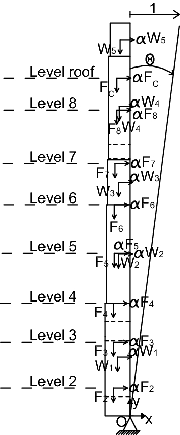

  

  Kinematic model for the mechanism A1: simple overturning of the entire South wall

• δ_y.i is the virtual vertical displacement of the point of application of the i-th weight-force.

Finally, the acceleration α₀ can be used to compute the specific mechanism acceleration capacity α₀* as follows:

$$a_{0}^{*} = \frac{{\alpha_{0} \mathop \sum \nolimits_{i = 1}^{n + m} m_{i} }}{{M^{*} F_{C} }} = \frac{{\alpha_{0} }}{{e^{*} F_{C} }}$$

(11)

where

• m_i is the mass of the generic block or floor;

• F_C is the confidence factor. The value of F_C used for the EL1 (F_C = 1.35) is also applied here as the same level of knowledge is used.

• $e^{*} = M^{*} /\mathop \sum \nolimits_{i = 1}^{n} m_{i}$ is the participating mass ratio of the considered mechanism.

• M* is the participating mass for the considered mechanism, obtained as a function of the horizontal virtual displacements as follows:

$$M^{*} = \frac{{\left( {\mathop \sum \nolimits_{i = 1}^{n + m} m_{i} \delta_{x,i} } \right)^{2} }}{{\mathop \sum \nolimits_{i = 1}^{n + m} m_{i} \delta_{x,i}^{2} }}$$

(12)

Compliance with SLV is verified for each mechanism if the acceleration factor:

$$f_{a,SLV} = \frac{{a_{0}^{*} }}{{a_{exp,SLV} }} > 1$$

(13)

According to Eq. (4), the seismic safety index I_S evaluated as the ratio between the return period of the life-safety seismic action, $T_{SLV}$, and the return period for which the SLV action should be satisfied $T_{R,SLV}$. In the context of kinematic analyses $T_{SLV}$ is obtained as the return period of the seismic action that leads to an acceleration factor $f_{a,SLV}$ = 1. The results are collated in Table 6 and summarized in Fig. 10.

Table 6 EL2—results in terms of: loads multiplier (α₀), return period of the collapse seismic action (T_SLV), nominal life (V_N), seismic safety index (I_S,SLV) and acceleration factor (f_a,SLV)

Fig. 10

Acceleration factors obtained for each mechanism

Overall, it can be concluded that:

• The simple overturning mechanisms (Type A) are generally the most dangerous, while the vertical flexural mechanism (Type D) is the least dangerous. Combined overturning mechanisms (type B) and overturning of the corner sections (Type C) present intermediate seismic vulnerabilities.

• In the case of overturning mechanisms, the higher is the location of the horizontal cylindrical hinge, the higher is the acceleration capacity α₀* of the mechanisms. Table 6 shows that the only mechanism activated for the expected ultimate limit state acceleration is the mechanism A1, which represent the simple overturning of the entire South wall. For this failure mode, the ratio between acceleration capacity and acceleration demand is $f_{a,SLV}$ = 0.45. Since the geometries of the East, West and South facades are substantially the same, the most likely out-of-plane failure mechanisms are the simple overturning of these three walls.

• However, these results must be interpreted with caution. This is because the assumption of completely ineffective connections between perpendicular walls, which determines simple overturning mechanisms (Type A), might represents a conservative hypothesis in the case of the Cugnanesi tower. In fact, the thickness of the walls, together with a visual inspection of the connections, and the lack of vertical cracks in these positions, suggests that the connection between vertical walls is quite robust. Hence, combined overturning mechanisms (Type B) and overturning of the corner sections (Type C) might represents more realistic failure modes and, consequently, provide more reliable seismic risk assessments.

5 Seismic risk assessment by EL3 approach

The evaluation level EL3 requires the assessment of the structure global seismic behaviour by means of global numerical models (PCM 2011). This assessment is here developed by performing non-linear static pushover analyses by means of non-linear Finite Element (FE) models of the Cugnanesi tower.

First, two linear elastic FE models of the tower having dynamic properties corresponding to the experimentally estimated ones were built. The two models capture the global elastic behaviour of the tower by modelling its multi-leaf walls as homogenous and layered solids respectively. The models were built and calibrated through a series of parametric analyses described in detail in Sect. 5.1.

Then, two non-linear models were considered by assigning an elastic-plastic material behaviour to the most representative configuration identified upon dynamic characterization (Sect. 5.2). The non-linear models were employed to perform pushover analyses with the aim to assess: (1) the sensitivity of the solution to the multi-leaf walls modelling strategy; (2) the global seismic performances of the structure. The purpose of this study is to show the implication in terms of effort and information needed to perform a reliable analysis at level EL3, compared with the two previous approaches.

5.1 Dynamic characterization

In order to tune FE models of the tower having dynamic properties corresponding to the experimentally measured ones, a series of linear parametric FE analyses have been carried out by the commercially available code Autodesk Simulation Multiphysics (Autodesk 2013). The masonry walls were discretised by eight-node isoparametric solid elements. The aims of these analyses were:

• To define a convenient mesh size for the FE model of the tower.

• To evaluate the sensitivity of the numerical dynamic behaviour of the structure with respect to the adjacent buildings modelling strategy.

• To analyse the influence of the soil–structure interaction on the dynamic behaviour of the entire system.

• To assess the elastic modulus of the tower and adjacent constructions.

• To explicitly model the multi-leaf walls as composed of various layers of different materials.

The assumed parameters are: (1) geometry of the tower; and (2) elastic properties of the soil, while the parameters calibrated by means of the iterative process of identification are: (1) elastic properties of the confining adjacent walls—lateral constraints; and (2) elastic properties of the tower.

5.1.1 Interaction between tower and adjacent buildings

With the aim of evaluating the sensitivity of the dynamic behaviour of the structure with respect to the adjacent buildings modelling strategy, three different numerical models were defined (Fig. 11):

• Model A: no adjacent building is modelled; hence, the tower is modelled as structurally independent. This model is analogous to Model A used for EL1, were the tower was assumed isolated (see Sect. 3).

• Model B: the adjacent buildings are modelled as infinitely rigid in their plane; the in-plane translational degrees of freedom of the nodes located on the contact surface between the tower and the walls of the adjacent building are fixed. This assumption is analogous to that of effectively constraining adjacent buildings made in Models B and C of EL1 (see Sect. 3).

• Model C: the adjacent buildings are explicitly modelled; their elastic properties are chosen according to the DRS material characteristics. Hence, the dynamic properties of this model are expected to lie between those of Models A and B defined above.

Fig. 11

Aerial view of the Cugnanesi (a) and axonometric view of models A (b), B (c) and C (d)

Based on a set of preliminary mesh sensitivity studies, a maximum elements size of 0.8 m is assumed for both tower and adjacent walls. For all the models the base is supposed fixed, and the elastic parameters of the tower are assumed according to the DRS material (see Table 1).

Among these three models, model C was assumed to be the one which better reproduces the real confining effect due to the adjacent buildings. The results, expressed in terms of modal frequencies, are reported in Fig. 12. Since the main frequency of the three models A, B and C ranges between 0.81 and 1.10 Hz, it is possible to conclude that the modelling strategy of the adjacent walls significantly influences the solution. It is also worth noting that the main frequencies of the three models are lower than the main frequency obtained through dynamic identification (Fig. 12). Even Model B, despite its limit-case assumption of infinitely rigid adjacent walls, predicts considerably lower frequencies than the experimental measurements. This confirms that the actual stiffness of the masonry is greater than that obtained with the material model DRS, which is the stiffest masonry type defined by MIT (2009) (E = 2800 MPa). For this reason, the elastic modulus of the FE model is changed to match the natural period (Sect. 5.1.3). Prior to calibrating the elastic modulus of the tower, an elastic model of the soil is introduced based on the results of a borehole performed near the tower (Madiai et al. 2017). The reason for introducing an elastic model of the soil prior to calibration of the tower elastic modulus is the relatively large amount of information available on the elastic properties of the soil (Madiai et al. 2017). In this way, the elastic properties of the soil are known, while the elastic modulus of the tower is varied to match the experimentally measured dynamic properties of the tower, including the effect of non-infinitely rigid soil and foundations.

Fig. 12

Comparison between experimentally and numerically estimated frequencies

5.1.2 Soil–structure interaction

To analyse the influence of the soil–structure interaction on the dynamic behaviour of the entire system, model C with explicitly modelled soil is used (see Fig. 13b). To contain the number of elements to be used to model the soil, the profiles elastic parameters based on the results of a borehole performed close to the tower (Madiai et al. 2017) are discretized. This allows to model the soil as series of three-meters-deep-layers having uniform elastic properties and lying on top of each other (see Fig. 14). A volume of soil having depth of about 45 m and horizontal width of about 55 m is modelled, these dimensions being comparable to the major dimension of the structure. The bottom and the lateral surfaces of the mass of soil are modelled as fixed. The comparison between the results obtained with and without soil reveals that the soil modelling strategy significantly influences the dynamic behaviour of the model. Indeed, a fundamental frequency of 0.97 Hz is obtained when the base of the model is assumed fixed, while a fundamental frequency of 0.93 Hz is computed if the soil is modelled explicitly (see Fig. 13).

Fig. 13

Comparison between frequencies obtained with and without soil model

Fig. 14

Profiles of E_DISCR and G_DISCR computed as the average values of E and G for each three-meters-deep layer

5.1.3 Elastic modulus of tower and adjacent walls

A set of different models are defined, obtained starting from Model C, by only modifying the stiffness of the tower, with the simplified assumption of a single equivalent homogeneous elastic material through the thickness, disregarding the multi-leaves structure of the wall. A reference elastic modulus of E = 2800 MPa is considered, corresponding to the stiffness of the DRS material defined by the MIT2009. This value was then varied in the range from 2800 to 9000 MPa, while maintaining constant the value of the Poisson’s ratio υ = 0.2. As shown by Fig. 15, the model which best fits the experimental first frequencies is the one with E = 8000 MPa for the masonry. Therefore, this value was adopted for the following analyses.

Fig. 15

First mode frequency versus tower masonry stiffness

The calibrated elastic parameters of soil and tower were then used to calibrate the equivalent elastic modulus of the adjacent walls. Figure 16 shows the value of the ratio between the first two natural frequencies as a function of the elastic modulus of the tower. Although the ratio between the first two frequencies is very close to the one obtained from experimental frequencies it is slightly underestimated by the numerical models. Therefore, a new series of parametric analyses, focused on estimating effective values for the elastic modulus of the adjacent walls, is performed. Since it was observed that the first frequency mainly depends on the East–West adjacent wall stiffness while the second frequency mainly depends on the North–South wall stiffness, the stiffness of the N–S adjacent wall is tuned by looking for the elastic modulus capable of producing a frequency $f_{1y}$ of 1.46 Hz (Fig. 17). Similarly, once fixed the elastic modulus of the N–S adjacent wall, E_NS = 3200 MPa, a sensitivity study is performed to find the elastic modulus of the East–West adjacent wall, E_EW = 2600 MPa, which causes a natural frequency $f_{1x}$ 1.31 Hz (Fig. 18).

Fig. 16

f₂/f₁ ratio versus tower masonry stiffness

Fig. 17

First modes frequencies versus N–S wall stiffness

Fig. 18

First modes frequencies versus E–W wall stiffness

5.1.4 Multi-leaf walls modelling method

In a multi-leaf wall, the relative thickness and mechanical properties of the single layers directly affect the stress distribution and ultimate capacity of the overall structure. Hence, accurate modelling of their layered structure is generally needed for reliable structural assessment. A FE model of the tower capable of describing the multilayer configuration of the walls was also calibrated, to investigate the influence of the walls modelling strategy on the results of global ultimate state seismic analysis. The geometry of the multi-leaf structure of the walls was evaluated assuming the external stone layers and the internal filling material having the same elastic properties experimentally determined for the “Torre Grossa” tower (Bartoli et al. 2013) (Table 7), a nearby tower in San Gimignano which presents constructive and materials characteristics similar to the tower here analysed. A sensitivity analysis was conducted to determine the influence of the relative thickness of the layers on the dynamic response of the tower (see Fig. 19). The elastic properties of external and internal layers were kept constant. The multi-leaf walls were modelled as a continuum, that is, perfect bond was assumed between the layers. As shown from Fig. 20, Model 1 presents frequencies similar to the ones of Model 2, while Model 3 presents frequencies similar to the ones of Model 4. In other words, the dynamic behaviour of the tower does not significantly depend on the thickness of the internal stone layer but it mainly depends on the thickness of the external stone layer. Indeed, since the first two modal shapes are flexural, the stiffness of the tower mainly depends on the bending stiffness of its horizontal sections, which in turn is not significantly influenced by the thickness of the internal stone layer, but primarily depends on the thickness of the external stone layer. Since Model 4 is the one which best fit the experimental results, a thickness of 0.5 m was adopted for both internal and external stone layers.

Table 7 Materials elastic properties

Fig. 19

Schematic representation of the different walls models

Fig. 20

First modes frequencies versus tower masonry structure

5.2 Pushover analyses

Once all relevant parameter in the elastic numerical model had been calibrated to optimise agreement with the dynamic identification natural frequencies values, a series of pushover analyses were performed to assess the global seismic performances of the structure and to evaluate the sensitivity of the solution with respect to the multi-leaf walls modelling strategy. Such analyses were carried out by using Ansys v.15 (Swanson Analysis Systems 2014).

The post elastic response of the masonry material was simulated by an elastic-perfectly plastic constitutive law with a Drucker–Prager failure criterion. In addition, to account for the masonry brittle tensile behaviour the Willam–Warnke failure cut-off surface was also considered (Betti et al. 2008, 2016). Figure 21 shows a schematic representation of the adopted criteria on the principal plane $\sigma_{1}$–$\sigma_{2}$. The combination of the Drucker–Prager plasticity model with the Willam–Warnke failure criterion allows for an elastic-brittle material behaviour in case of biaxial tensile stresses (segments 4–5 and 5–6 in Fig. 21) or biaxial tensile-compressive stresses with a relatively low compression level (segments 3–4 and 6–7). On the contrary, the material behaves as elastic-plastic in the case of biaxial tensile-compressive stresses with a relatively high compression level (segments 2–3 and 7–8 in Fig. 21) or biaxial compressive stresses (segments 1–2 and 8–9). Overall, the material behaves as an isotropic medium with plastic deformation, cracking and crushing capabilities. Both models have been extensively used in the scientific literature to model the post-elastic behaviour of masonry (Cerioni et al. 1995; Betti et al. 2015a, b). Due to the lack of experimental data on the materials, the DP and WW material parameters are selected in order to obtain the compressive and tensile strength experimentally measured for the nearby tower Torre Grossa (Bartoli et al. 2013). All material parameters are summarised in Table 8. For the elastic material parameters, the values calibrated within the dynamic identification reported in the previous section are adopted.

Fig. 21

Adopted material model: Drucker–Prager yield surface with Willam–Warnke cut-off in tension

Table 8 Selected elastic, DP and WW parameters ($E_{eq}$ = elastic modulus of the equivalent homogeneous walls, $E_{ext}$ = elastic modulus of the external layers of the multi-leaf walls, $E_{int}$ = elastic modulus of the core layer of the multi-leaf walls, $\varPhi$ = internal friction angle; δ = dilatancy angle; c = cohesion; f_wc = masonry compressive strength; f_wt = masonry tensile strength; β_c = shear transfer coefficient for closed cracks; β_t = shear transfer coefficient for open cracks)

The soil is modelled as a series of elastic layers, as described in Sect. 5.1. The uncertainties about the interaction with the adjacent buildings are taken into consideration by defining two limit models of the structural system: an Isolated Model (IM) (see Fig. 22a), to predict the behaviour of the tower in the case of collapse of the adjacent walls, analysed in North, South, West and East directions; a Complete Model (CM) where both the tower and the adjacent walls are modelled (see Fig. 22b) to study the constrained offered by the adjacent walls. The hypothesis is that the constraint is only effective when the connection is in compression, hence only the seismic directions North and West have been considered for this model as shown in Fig. 22b. Moreover, the effect of the adopted multi-leaf wall modelling strategy on the results of pushover analyses is also evaluated by considering an equivalent homogenized model, and the multi-leaf walls configuration of Model 4 (see Fig. 19d).

Fig. 22

Analysed seismic direction for a Isolated Model (IM) and b Complete Model (CM)

The pushover analyses are solved through a Newton–Raphson force-control numerical scheme (Swanson Analysis Systems 2014). The force-control scheme allows only the ascending branch of the pushover curve to be captured. Hence, the analyses stop at the limit point where extensive material damage leads to a null tangent matrix, thereby preventing numerical convergence.

The capacity curves obtained for these models with respect to different seismic load directions are reported in Fig. 23. The figure shows that the choice of the walls layers modelling method has negligible influence on the performance of the structure, with the two models showing similar yielding points and post elastic behaviour. In light of this, the non-linear analyses aimed at assessing the global seismic behaviour of the structures are performed by using the equivalent smeared models.

Fig. 23

Capacity curves for different wall layers modelling methods and seismic action in the a North-direction, b East-direction, c West-direction, d South-direction

The capacity curves obtained for each different analyses are reported in Fig. 24. As expected, the Complete Model (CM) shows greater global stiffness and strength than the isolated one, and a slightly lower displacement capacity for westbound and northbound seismic actions. The Isolated Model (IM) exhibits relatively high displacement capacities in all the analysed directions, except for southbound seismic action. All the models exhibit a flexural failure mechanism. The premature collapse of the Isolated Model (IM) subjected to southbound seismic action is due to the development of high tensile vertical stresses in the North wall of the tower at a height of about 8.50 m from the ground level (see Fig. 25a), where both the South and the West walls present openings (see block 5 in Fig. 4). Neither the simplified mechanical analyses (EL1) nor the mechanism approach (EL2) allowed this failure mode to be captured. Indeed, the simplified mechanical analyses according to EL1 predicted the base section of the tower to fail first. Similarly, this failure mode was not captured through mechanism analyses (EL2). In the case in Complete Model (CM), flexural failure occurs because of extensive damage of the sections around the upper bound of the lateral walls. As an example, Fig. 25b shows that in the case of Complete Model and westbound seismic action the highest tensile stresses develop in the East wall at a height of about 16.00 m. This is in line the adoption of the simplified mechanical models A and B considered within the EL1 (see Sect. 3), where the portion of the tower that emerges from the surrounding buildings was considered as a cantilever beam.

Fig. 24

Capacity curves obtained for the push over analysis of the isolated and constrained model

Fig. 25

Maximum principal stresses contour diagrams: a Isolated Model (IM) subjected to southbound seismic action and b Complete Model (CM) subjected to westbound seismic action. Deformed shapes corresponding to a scale factor of 50

The results of the pushover analyses were then used to perform seismic safety check according to the N2 method, proposed by Fajfar and Gašperšič (1996), extended to applications to historic buildings (D’Ayala and Ansal 2012; D’Ayala et al. 2015; Giordano et al. 2019). The process consists of obtaining the appropriate inelastic response, i.e. the performance point (defined as point of intersection of an idealized bilinear SDOF capacity curve with the inelastic demand spectrum) for the given seismic action.

First, each pushover curve was reduced to the response of an equivalent nonlinear SDOF system. The forces $F^{ *}$ and the displacements $d^{ *}$ of the equivalent SDOF system were obtained as:

$$F^{ *} = \frac{V}{\varGamma }$$

(14)

$$d^{ *} = \frac{u}{\varGamma }$$

(15)

where $V$ and $u$ are the forces and displacements of the MDOF FE model respectively, and $\varGamma$ is the modal participation factor (Fajfar and Gašperšič 1996). Then, the idealized bilinear SDOF capacity curve is obtained with the stiffness $k^{ *}$ of the elastic-plastic SDOF is determined as:

$$k^{ *} = \frac{{0.6 F_{bu}^{ *} }}{{u\left( {0.6 {\text{F}}_{bu}^{ *} } \right)}}$$

(16)

computed at 60% of $F_{bu}^{ *}$, where $F_{bu}^{ *}$ is the ultimate base shear of the nonlinear SDOF capacity curve (MIT 2009). The yield force of the idealised SDOF capacity curve is determined following the equal energy assumption.

Figures 26 and 27 show the SLV performance points for all the analysed conditions. For each condition, the displacement demand $d_{SLV}$ defined by the performance point is compared with the corresponding SLV capacity displacement $d_{u,SLV}$, obtained as (MIT 2019):

$$d_{u,SLV} = 0.75 d_{u,col}$$

(17)

where $d_{u,col}$ is the collapse capacity displacement, identified by the rightmost point of the SDOF capacity curve. For each case, the return period $T_{SLV}$ of the SLV seismic action is obtained as the return period that causes the demand displacement to equal the capacity displacement:

$$d_{SLV} = d_{u,SLV}$$

(18)

Fig. 26

Isolated models: elastic demand spectrum, SDOF elastic-plastic capacity curves and corresponding inelastic demand spectra (for T_R = 475y). The SLV performance points are represented by circles

Fig. 27

Complete models: elastic demand spectrum, SDOF elastic-plastic capacity curves and corresponding inelastic demand spectra (for T_R = 475y). The SLV performance points are represented by circles

As an example, Fig. 28 illustrates the SDOF capacity curve of the isolated model subjected to seismic action directed towards South, the elastic and inelastic demand spectra corresponding to $T_{R}$ = 475 years and $T_{SLV} =$ 680 years, the corresponding SLV performance point, and the Collapse and SLV damage thresholds. The figure shows that, for this particular scenario, the SLV performance point check is satisfied: the capacity displacement is greater than the corresponding displacement demand.

Fig. 28

Isolated model subjected to seismic action directed towards South: capacity curve, elastic and inelastic demand spectra for T_R = 475y and T_R = 680 y, collapse and SLV damage thresholds, and SLV performance point

For each considered condition, seismic safety index $I_{S,SLV}$ and acceleration factor $f_{a,SLV}$ are computed using Eqs. (4) and (6). In the context of the evaluation level EL3, $I_{S,SLV}$ and $f_{a,SLV}$ are obtained by assuming a confidence factor F_C = 1, corresponding to a knowledge level KL3. This is because the numerical models adopted within the EL3 are built in light of accurate geometrical surveys, in-situ checks of constructive details and material properties, and non-destructive interferometric radar measurements to assess the dynamic properties of the tower.

Table 9 summarizes the results obtained for all the analysed conditions in terms of period $T^{*}$ of the idealised SDOF bilinear curve, return period $T_{SLV}$ of the SLV seismic action, collapse capacity displacement $d_{u,col}$, SLV capacity displacement $d_{u,SLV}$, SLV demand displacement $d_{SLV}$, seismic safety index $I_{S,SLV}$ and acceleration factor $f_{a,SLV}$. The table shows that the performance point checks are satisfied for all the considered scenarios. Overall, the performed Capacity Spectrum Method (CSM) checks and the obtained safety indexes reveal that the tower has good safety margins against ultimate limit state seismic events.

Table 9 EL3—results in terms of: period of the idealised SDOF bilinear curve (T*), return period of the collapse seismic action (T_SLV), collapse capacity displacement (d_u,col), SLV capacity displacement (d_u,SLV), SLV demand displacement (d_SLV), seismic safety index (I_S,SLV) and acceleration factor (f_a,SLV)

A cross-interpretation of the three evaluation levels EL1, EL2 and EL3 indicates that over conservative assessments are obtained with both EL1 and EL2 approaches, where a relatively low knowledge level of the structure (KL1) was assumed. A comparison between EL1 and EL3 (see Tables 5 and 9 respectively) shows that significantly lower safety margins are computed through EL1 analyses. That is, EL1 approach leads to conservative assessments. This is partly because the material strength suggested by the Italian Recommendations employed for EL1 analyses is substantially lower than the actual strength of the tower. Indeed, these recommendations are meant for ordinary masonry structures, such as modest height buildings, while masonry towers, such as the Cugnanesi, should be considered as monumental and highly engineered buildings for their time. If the compressive strength considered in EL3 ($f_{m}$ = 8 MPa) were used in EL1, more comparable results would be obtained. Specifically, $f_{a,SLV}$ = 1.44 and $I_{S}$ = 3.47 would be obtained in EL1 for Model A subjected to seismic action directed toward North. Part of the difference between the predictions obtained by EL1 and EL3 can also be attributed to the fact that within EL1 the assumption of relatively low knowledge level of the structure (KL1) results in a confidence factors F_C = 1.35, while the assumption of relatively high knowledge level of the structure (KL3) within EL3 leads to a confidence factor F_C = 1.

Significantly conservative results are also obtained if only mechanism analyses (EL2) are carried out for individual façades (Model A, see Table 6). As with EL1 analyses, the safety margins computed within EL2 are influenced by the assumption of low knowledge level of the structure (KL1) that results in a confidence factors F_C = 1.35. Furthermore, relatively low safety indices are obtained due to the assumption of zero tensile strength at the interfaces between different rigid blocks. Indeed, such assumption may lead to significantly conservative assessments in the case of structures with good masonry quality and mechanism involving relatively large contact surfaces between the assumed blocks. This is because the fracture energy required to generate a given contact surface grows with the quality of the material and with the area of the surface itself. It is worth noting that when efficient connections between perpendicular walls are considered (mechanisms type B and C), seismic safety indices comparable to those obtained within EL3 are computed.

6 Concluding remarks

The paper discusses the seismic assessment methods proposed by the Italian Guidelines (PCM 2011) for the assessment and mitigation of the seismic risk of cultural heritage buildings. As a reference case, the illustrative medieval Cugnanesi tower located in San Gimignano (Italy) is investigated.

The following conclusions can be drawn from the present study:

• The seismic safety indexes (acceleration factor and seismic safety index) obtained with the analysis at the territorial scale (EL1) are confirmed by the results obtained with the EL3 approach.

• The EL3 safety indexes are always greater than those obtained with the EL1, showing a general coherence between the two approaches. It is however worth noting that these two approaches are not alternative to each other but belong to two different levels of evaluation and therefore more conservative results were actually expected for the latter with respect to the former evaluation method.

• Among the collapse mechanisms analysed within the evaluation level EL2, the most critical ones are the overturning failure modes of the individual facades. Therefore, the effectiveness of connections between orthogonal walls should always be carefully considered when assessing slender masonry towers.

• The presence of surrounding buildings, here assessed by analysing two limit cases (isolated model, IM and complete model, CM), strongly affects the dynamic behaviour, and therefore the seismic performances, of the examined tower. Thus, it is essential to assess the constraining effect provided by the adjacent buildings when performing EL3 assessment of confined masonry towers.

• If the soil is modelled explicitly by means of a series of elastic layer on top of each other, a more flexible FE model is obtained than the one with fixed base. Hence, it is generally crucial to gather as much information as possible on the mechanical parameters of the soil and to model it explicitly. This is an important aspect that significantly affects the nonlinear behaviour of historic towers, which must be taken into account when time-history analyses are performed, even if it is expected that the presence of lateral restraints attenuates the effect of the soil–structure interaction.

• For the examined tower, the adopted distribution of elastic properties across the horizontal section of multi-leaf walls of masonry does not significantly affect the results of global pushover analyses (EL3). This legitimates the use of models having equivalent homogenized elastic stiffness in the case of lack of detailed structural surveys.

• Different failure modes were predicted by the three evaluation levels EL1, EL2 and EL3. Thus, it is generally necessary to develop all the approaches to have a comprehensive understanding of the possible seismic performance of masonry towers. The paper suggests that comparing different approaches for the analysis of historic towers in conjunction with parametric analyses is mandatory in order to cover the unavoidable unknowns that always affect the construction and the analysis approaches.

• Over conservative assessments were obtained with both EL1 and EL2 approaches. This is partly due to the level of knowledge of the structure. In this study, a low knowledge level (KL1) was assumed for EL1 and EL2 analyses. By contrast, an accurate knowledge level (KL3) was assumed for EL3, where detailed information on geometry, materials, and structural details were used. Accordingly, a confidence factor F_C = 1.35 was assumed for EL1 and EL2 analyses, whereas F_C = 1 was used within EL3.

• The relatively low safety margins computed through EL1 analyses are also due to the afore-mentioned underestimation of material strength obtained through the Italian recommendations. If the material strength considered in EL3 were used in EL1, more comparable results would be obtained.

• The relatively low safety margins computed through EL1 analyses can also be attributed to the assumption of the assumption of zero tensile strength at the interfaces between different rigid blocks. Indeed, such assumption may lead to significantly conservative assessments in the case of structures with good quality masonry and extensive interfaces between the assumed blocks. This is the case for the mechanisms of overturning of the facades of the studied tower. Hence, the analyst should judge which type of mechanisms is the most appropriate for the given structural conditions.

References

Acito M, Bocciarelli M, Chesi C, Milani G (2014) Collapse of the clock tower in Finale Emilia after the May 2012 Emilia Romagna earthquake sequence: numerical insight. Eng Struct 72:70–91
Atzeni C, Bicci A, Dei D et al (2010) Remote survey of the leaning tower of Pisa by interferometric sensing. IEEE Geosci Remote Sens Lett 7:185–189
Autodesk (2013) Autodesk simulation multuphysics—simulation mechanical, v.2013. User’s guide: https://knowledge.autodesk.com/support/simulation-mechanical
Bartoli G, Betti M (2018) Seismic risk of monumental buildings: outcomes of the research project RiSEM. J Perform Constr Facil. https://doi.org/10.1061/(ASCE)CF.1943-5509.0001193
Bartoli G, Betti M, Spinelli P, Tordini B (2006) An “innovative” procedure for assessing the seismic capacity of historical tall buildings: the “ Torre Grossa ” masonry tower. Proc V Int Conf Struct Anal Hist Constr SAHC 2006 929–937
Bartoli G, Betti M, Giordano S (2013) In situ static and dynamic investigations on the “Torre Grossa” masonry tower. Eng Struct 52:718–733
Bartoli G, Betti M, Vignoli A (2016) A numerical study on seismic risk assessment of historic masonry towers: a case study in San Gimignano. Bull Earthq Eng 14:1475–1518
Bartoli G, Betti M, Galano L, Zini G (2019) Numerical insights on the seismic risk of confined masonry towers. Eng Struct 180:713–727. https://doi.org/10.1016/J.ENGSTRUCT.2018.10.001
Betti M, Galano L, Vignoli A (2016) Finite element modelling for seismic assessment of historic masonry buildings. In: D'Amico S (eds) Earthquakes and their impact on society. Springer Natural Hazards. Springer, Cham. https://doi.org/10.1007/978-3-319-21753-6_14
Betti M, Galano L, Petracchi M, Vignoli A (2015a) Diagonal cracking shear strength of unreinforced masonry panels: a correction proposal of the b shape factor. Bull Earthq Eng 13:3151–3186. https://doi.org/10.1007/s10518-015-9756-8
Betti M, Galano L, Vignoli A (2015b) Time-history seismic analysis of Masonry buildings: a comparison between two non-linear modelling approaches. Buildings 5:597–621. https://doi.org/10.3390/buildings5020597
Betti M, Galano L, Vignoli A (2016) Finite element modelling for seismic assessment of historic masonry buildings. In: Earthquakes and their impact on society. Springer, Berlin, pp 377–415
Bowitz E, Ibenholt K (2009) Economic impacts of cultural heritage–research and perspectives. J Cult Herit 10:1–8
Brandonisio G, Lucibello G, Mele E, De Luca A (2013) Damage and performance evaluation of masonry churches in the 2009 L’Aquila earthquake. Eng Fail Anal 34:693–714
Casolo S, Milani G, Uva G, Alessandri C (2013) Comparative seismic vulnerability analysis on ten masonry towers in the coastal Po Valley in Italy. Eng Struct 49:465–490
CEN (2005) BS EN 1998-1:2004+A1:2013. Eurocode 8: design of structures for earthquake resistance—part 1: general rules, seismic actions and rules for buildings. Eur Stand
Cerioni R, Brighenti R, Donida G (1995) Use of incompatible displacement modes in a finite element model to analyze the dynamic behavior of unreinforced masonry panels. Comput Struct 57:47–57. https://doi.org/10.1016/0045-7949(94)00590-Y
Ceroni F, Pecce M, Manfredi G (2009) Seismic assessment of the bell tower of Santa Maria Del Carmine: problems and solutions. J Earthq Eng 14:30–56
Chiozzi A, Grillanda N, Milani G, Tralli A (2018) UB-ALMANAC: an adaptive limit analysis NURBS-based program for the automatic assessment of partial failure mechanisms in masonry churches. Eng Fail Anal 85:201–220. https://doi.org/10.1016/J.ENGFAILANAL.2017.11.013
Clementi F, Pierdicca A, Formisano A et al (2017) Numerical model upgrading of a historical masonry building damaged during the 2016 Italian earthquakes: the case study of the Podestà palace in Montelupone (Italy). J Civ Struct Heal Monit 7:703–717. https://doi.org/10.1007/s13349-017-0253-4
Clementi F, Ferrante A, Giordano E et al (2019) Damage assessment of ancient masonry churches stroked by the Central Italy earthquakes of 2016 by the non-smooth contact dynamics method. Bull Earthq Eng. https://doi.org/10.1007/s10518-019-00613-4
D’Ambrisi A, Mariani V, Mezzi M (2012) Seismic assessment of a historical masonry tower with nonlinear static and dynamic analyses tuned on ambient vibration tests. Eng Struct 36:210–219
D’Ayala D (2014) Conservation principles and performance based strengthening of heritage buildings in post-event reconstruction. In: Ansal A (eds) Perspectives on European earthquake engineering and seismology. vol 34. Geotechnical, Geological and Earthquake Engineering, Springer, Cham. https://doi.org/10.1007/978-3-319-07118-3_15
D’Ayala D (ed) (2019) The MW 6.2 Amatrice, Italy earthquake of 24 August 2016, a field report by EEFIT. https://www.istructe.org/IStructE/media/Public/Resources/report-eefit-mission-italy-20190501.pdf
D’Ayala D, Ansal A (2012) Non linear push over assessment of heritage buildings in Istanbul to define seismic risk. Bull Earthq Eng 10:285–306. https://doi.org/10.1007/s10518-011-9311-1
D’Ayala D, Speranza E (2003) Definition of collapse mechanisms and seismic vulnerability of historic masonry buildings. Earthq Spectra 19:479–509. https://doi.org/10.1193/1.1599896
D’Ayala D, Meslem A, Vamvatsikos D, Porter K, Rossetto T, Silva V (2015) Guidelines for analytical vulnerability assessment of low/mid-rise buildings, vulnerability global component project. https://doi.org/10.13117/GEM.VULN-MOD.TR2014.12
D’Ayala D, Alexander D, De Luca F et al (2017) Earthquake Engineering Field Investigation Team (UK)—Data and discussion on the 2016 Central Italy Mission. In: 16th World conference on earthquake engineering (16WCEE). 16th World Conference on Earthquake Engineering (16WCEE)
Delanty G, Jones PR (2002) European identity and architecture. Eur J Soc Theory 5:453–466
Faccio P, Podestà S, Saetta A (2011) Venezia, Campanile della Chiesa di Sant’Antonin, Esempio 5, in Linee Guida per la valutazione e riduzione del rischio sismico del patrimonio culturale allineate alle nuove Norme tecniche per le costruzioni (D.M. 14/01/2008), Circolare 26/2010 (in Italian)
Fajfar P, Gašperšič P (1996) The N2 method for the seismic damage analysis of RC buildings. Earthq Eng Struct Dyn 25:31–46
Fioravanti M, Mecca S (2011) The safeguard of cultural heritage: a challenge from the past for the europe of tomorrow: COST strategic workshop, July 11th–13th, 2011, Florence. Firenze University Press, Italy
Fratini M, Pieraccini M, Atzeni C et al (2011) Assessment of vibration reduction on the Baptistery of San Giovanni in Florence (Italy) after vehicular traffic block. J Cult Herit 12:323–328
Gentile C, Saisi A (2007) Ambient vibration testing of historic masonry towers for structural identification and damage assessment. Constr Build Mater 21:1311–1321
Giordano E, Clementi F, Nespeca A, Lenci S (2019) Damage assessment by numerical modeling of Sant’Agostino’s Sanctuary in offida during the central Italy 2016–2017 seismic sequence. Front Built Environ 4:87
Giorgi L, Matracchi P (2017) Architectural evolution: modifications, alterations, and restorations through centuries. J Perform Constr Facil 31:4017046. https://doi.org/10.1061/(ASCE)CF.1943-5509.0001014
ICOMOS/Iscarsah (2005) Recommendations for the analysis, conservation and structural restoration of architectural heritage. www.icomos.org
ISO (2010) ISO 13822: 2010. Bases for design of structures: assessment of existing structures
Ivorra S, Pallarés FJ, Adam JM (2009) Experimental and numerical results from the seismic study of a masonry bell tower. Adv Struct Eng 12:287–293
Madiai C, Renzi S, Vannucchi G (2017) Geotechnical aspects in seismic soil–structure interaction of San Gimignano towers: probabilistic approach. J Perform Constr Facil 31:4017059. https://doi.org/10.1061/(ASCE)CF.1943-5509.0001041
MDF (2009) NCSE-02: Norma de Construcción Sismorresistente: Parte General y Edificación—Ministerio de Fomento, Gobierno de España (in Spanish)
Milani G (2019) Vulnerability evaluation of historical masonry structures: Italian churches and towers. In: Aguilar R, Torrealva D, Moreira S et al (eds) Structural analysis of historical constructions. Springer International Publishing, Cham, pp 19–32
Milani G, Casolo S, Naliato A, Tralli A (2012) Seismic assessment of a medieval masonry tower in Northern Italy by limit, nonlinear static, and full dynamic analyses. Int J Archit Herit 6:489–524
Milani G, Shehu R, Valente M (2017) Role of inclination in the seismic vulnerability of bell towers: FE models and simplified approaches. Bull Earthq Eng 15:1707–1737. https://doi.org/10.1007/s10518-016-0043-0
MIT (2008) NTC 2008: D.M. del Ministero delle Infrastrutture e dei Trasporti del 14/01/2008. Nuove Norme Tecniche per le Costruzioni. G.U. n. 29 del 04.02.2008, S.O. n. 30 (in Italian)
MIT (2009) Circolare n. 617 del 2 febbraio 2009 del Ministero delle Infrastrutture e dei Trasporti. Istruzioni per l’applicazione delle Nuove Norme Tecniche delle Costruzioni di cui al Decreto Ministeriale 14gennaio 2008 (in Italian)
MIT (2018) NTC 2018: D.M. del Ministero delle Infrastrutture e dei trasporti del 17/01/2018. Aggiornamento delle Norme Tecniche per le Costruzioni (in Italian)
MIT (2019) Circolare n. 7 del 21 gennaio 2019 del Ministero delle Infrastrutture e dei Trasporti. Istruzioni per l’applicazione dell’«Aggiornamento delle “Norme tecniche per le costruzioni”» di cui al decreto ministeriale 17 gennaio 2018 (in Italian)
Novelli VI, D’Ayala D, Makhloufi N et al (2015) A procedure for the identification of the seismic vulnerability at territorial scale. Application to the Casbah of Algiers. Bull Earthq Eng 13:177–202. https://doi.org/10.1007/s10518-014-9666-1
PCM (2003) OPCM 3274: Ordinanza del Presidente del Consiglio dei Ministri 20 marzo 2003. Criteri per l’individuazione delle zone sismiche—Individuazione, formazione e aggiornamento degli elenchi nelle medesime zone. G.U. n 105 (in Italian)
PCM (2011) DPCM 2011: Direttiva del Presidente del Consiglio dei Ministri per valutazione e riduzione del rischio sismico del patrimonio culturale con riferimento alle norme tecniche per le costruzioni, G.U. n. 47 (in Italian)
Pieraccini M (2017) Extensive measurement campaign using interferometric radar. J Perform Constr Facil 31:4016113. https://doi.org/10.1061/(ASCE)CF.1943-5509.0000987
Pieraccini M, Fratini M, Parrini F, Atzeni C (2006) Dynamic monitoring of bridges using a high-speed coherent radar. IEEE Trans Geosci Remote Sens 44:3284–3288
Pieraccini M, Dei D, Betti M et al (2014) Dynamic identification of historic masonry towers through an expeditious and no-contact approach: application to the “Torre del Mangia” in Siena (Italy). J Cult Herit 15:275–282
Pieraccini M, Betti M, Forcellini D et al (2017) Radar detection of pedestrian-induced vibrations on Michelangelo’s David. PLoS ONE 12:e0174480
Poiani M, Gazzani V, Clementi F et al (2018) Iconic crumbling of the clock tower in Amatrice after 2016 central Italy seismic sequence: advanced numerical insight. Procedia Struct Integr 11:314–321. https://doi.org/10.1016/j.prostr.2018.11.041
Rainieri C, Fabbrocino G (2011) Il periodo elastico delle torri in muratura: correlazioni empiriche per la previsione. In: XIV Congresso Nazionale L’Ingegneria Sismica in Italia, Bari, pp 18–22
Russo G, Bergamo O, Damiani L, Lugato D (2010) Experimental analysis of the “Saint Andrea” Masonry Bell Tower in Venice. A new method for the determination of “Tower Global Young’s Modulus E”. Eng Struct 32:353–360
Sarhosis V, Milani G, Formisano A, Fabbrocino F (2018) Evaluation of different approaches for the estimation of the seismic vulnerability of masonry towers. Bull Earthq Eng 16:1511–1545. https://doi.org/10.1007/s10518-017-0258-8
Stewart J, Lanzo G, Aversa S et al (2016) Engineering reconnaissance of the 24 August 2016 Central Italy Earthquake. Version 2
Swanson Analysis Systems (2014) Ansys 15.0.7. User’s manual: https://www.sharcnet.ca/Software/Ansys/15.0.7/en-us/help/wb_sim/ds_Home.html
Tucci G, Bonora V (2017) Towers in San Gimignano: metric Survey Approach. J Perform Constr Facil. https://doi.org/10.1061/(ASCE)CF.1943-5509.0001085
UNESCO (2018) UNESCO World heritage centre: http://whc.unesco.org/en/list/. Accessed 10 Oct 2018
Valente M, Milani G (2016a) Seismic assessment of historical masonry towers by means of simplified approaches and standard FEM. Constr Build Mater 108:74–104
Valente M, Milani G (2016b) Non-linear dynamic and static analyses on eight historical masonry towers in the North-East of Italy. Eng Struct 114:241–270. https://doi.org/10.1016/J.ENGSTRUCT.2016.02.004
Acknowledgements
The authors kindly acknowledge the Tuscany Regional Administration that financially supported the research (theme PAR FAS 2007–2013—CIPE n°166/2007—line 1.1.a.3: Science and Technology for the preservation and enhancement of cultural heritage).
Author information
Authors and Affiliations
Corresponding author
Additional information
Publisher's Note
Springer Nature remains neutral with regard to jurisdictional claims in published maps and institutional affiliations.
Rights and permissions
Open Access This article is distributed under the terms of the Creative Commons Attribution 4.0 International License (http://creativecommons.org/licenses/by/4.0/), which permits unrestricted use, distribution, and reproduction in any medium, provided you give appropriate credit to the original author(s) and the source, provide a link to the Creative Commons license, and indicate if changes were made.
About this article
Cite this article
Torelli, G., D’Ayala, D., Betti, M. et al. Analytical and numerical seismic assessment of heritage masonry towers. Bull Earthquake Eng 18, 969–1008 (2020). https://doi.org/10.1007/s10518-019-00732-y
Received:
Accepted:
Published:
Issue Date:
DOI: https://doi.org/10.1007/s10518-019-00732-y