A cross-technology benchmark for incremental graph queries

Abstract

To cope with the increased complexity of systems, models are used to capture what is considered the essence of a system. Such models are typically represented as a graph, which is queried to gain insight into the modelled system. Often, the results of these queries need to be adjusted according to updated requirements and are therefore a subject of maintenance activities. It is thus necessary to support writing model queries with adequate languages. However, in order to stay meaningful, the analysis results need to be refreshed as soon as the underlying models change. Therefore, a good execution speed is mandatory in order to cope with frequent model changes. In this paper, we propose a benchmark to assess model query technologies in the presence of model change sequences in the domain of social media. We present solutions to this benchmark in a variety of 11 different tools and compare them with respect to explicitness of incrementalization, asymptotic complexity and performance.

1 Introduction

Models are a highly valuable asset in any engineering process as they capture the knowledge of a system in a formal abstraction. This abstraction allows to reason on properties in order to obtain insights on the underlying physical system through analysis.

These insights need to be refreshed as soon as the models of the system change in order to stay meaningful. However, for large systems it is often not viable to recalculate the entire model analysis for every change. Rather, it is desirable to propagate these changes to the analysis results incrementally, i.e. only recalculate those parts of the analysis results that are affected by a given change.

Requirements regarding these insights often change over time. This makes it very important to express such analyses in a maintainable and understandable form. Recently, multiple model query technologies [8, 9, 18, 46, 65] have been proposed to aid this problem by deriving an incremental change propagation from a declarative specification. Further, of course one could also use existing and established non-incremental query technology, particularly if some parts of the analysis are more complex and may not be supported by tools that target incremental change propagation. Finally, it is also an option to translate the model into dedicated analysis methods to reuse query technology not based on models. Given this plethora of options, it is difficult to estimate the differences and find the trade-offs between these approaches in terms of understandability, conciseness, efficiency and others. Does the tool fit into my technology space? Is it useful to rely on the incrementalization of a tool or is it better—at least performance-wise—to implement change propagation explicitly? How long does it take to recover from an application crash? How much development effort will be necessary to implement change propagation? How does it scale? Can I speed it up by adding more CPU cores? Is the tool extensible or can it happen that my analysis is not supported at some point?¹

To aid this comparison and assess how current modelling technologies are capable of offering a concise and understandable language for model analysis, yet still offer a good performance in the presence of frequent model changes, we propose the “Social Media” benchmark. In this benchmark, two queries should be formulated that analyse a model of a social media network. In social networks, new $\textsf {Post}$s , $\textsf {Comment}$s and likes arrive at a very high frequency and thus cause analyses of the entire network to invalidate quickly. In our benchmark, the analyses shall find the most influential posts and comments, according to selected criteria. While the first query is rather simple in the sense that it can easily be solved with standard query operators, the second query is more complex as graph algorithms are used that are not directly supported by query technologies.

Graph queries are difficult from an incrementalization point of view [31] as they capture a rich family of algorithms and they are often described in an imperative pseudo-code that usually utilizes state. Using a generic incrementalization system, this often spans a state space that is too large for an incrementalization to be efficient. To aid this situation, dynamic algorithms are known for a number of graph problems that offer strategies to propagate graph changes efficiently, often with a radically different approach than how with the computation was performed in the batch (or initial) scenario. However, there is no comparison yet how and how efficient such dynamic algorithms can be included into incremental query technologies.

We collected 11 implementations of this benchmark that cover most of the possible approaches mentioned above and have mostly been created by authors or active developers of the respective tools. Therefore, we claim that we can compare the tools through the solutions for this benchmark. The tools cover a wide area of model query technology and database management systems; thus, the analysis of the solutions using those tools allows us to reason on the previously mentioned questions.

The benchmark was originally proposed at the Transformation Tool Contest (TTC) 2018 as live contest [51]. At the TTC, several solutions have been submitted [12, 17, 34, 49, 78]. After the TTC, we invited further researchers working in incremental query technology to provide solutions in their favourite tools. In this paper, we present all of these solutions and compare them with respect to their features, complexity of change propagation and overall performance.

The remainder of this paper is structured as follows: Sect. 2 presents the benchmark and the queries that it consists of. Section 3 explains the solutions. Section 4 compares the solutions with respect to the declarativeness of the query language, the used data model, the explicitness of the incrementalization, the durability, support for parallelism and the asymptotic complexity of change propagations. Section 5 presents experimental performance results and their analysis. Section 6 discusses related work, and Sect. 7 concludes the paper.

Fig. 1

Metamodel (graph schema) of the social network model

2 The social media benchmark

In this section, we present the benchmark which we use to compare existing incrementalization approaches. First, Sect. 2.1 explains the metamodel that we use to model a social network graph, and then, Sect. 2.2 presents the two queries used in the benchmark. We describe the change sequences in Sect. 2.3 and the phases of the benchmark in Sect. 2.4.

2.1 Metamodel and change sequences

In this benchmark, we use the data from the 2016 DEBS Grand Challenge,² adapted from the LDBC Social Network Benchmark [5, 30] and the SIGMOD 2014 Programming Contest [27]. For this version of the benchmark, we created an Ecore metamodel to describe the social network, translated the series of events in the original data sources to models and change sequences and manually tuned the obtained change sequences.³

The metamodel of the social network is depicted in Fig. 1. The social network consists of $\textsf {User}$s, $\textsf {Post}$s and $\textsf {Comment}$s. $\textsf {User}$s may have $\textsf {friends}$, which is a unidirectional edge (i.e. it behaves as a symmetric relationship). $\textsf {Submission}$s form a tree with a $\textsf {Post}$ in its root and $\textsf {Comment}$s as the rest of its nodes. $\textsf {User}$s may like $\textsf {Comment}$s ($\textsf {likes}$ edge).

2.2 Queries

In the scope of the proposed benchmark, we focus on two model queries. The first query (Q1) is rather easy and is expected to be directly supported by the tools. It shall return the most controversial $\textsf {Post}$s in the social media network. The second query (Q2) is more sophisticated, and we expected it not to be directly supported by tools and force the solutions into case-specific extensions. It shall return the most influential $\textsf {Comment}$s. The results of both queries are concatenated to strings in order to use them for automated correctness checks.

2.2.1 Query 1: Most controversial posts

We consider a $\textsf {Post}$ as controversial, if it starts a debate through its $\textsf {Comment}$s. For this, we assign a score of 10 for each $\textsf {Comment}$ that belongs to a $\textsf {Post}$. Hereby, we consider a $\textsf {Comment}$ belonging to a $\textsf {Post}$, if it is a reply to either (1) the $\textsf {Post}$ itself or (2) another $\textsf {Comment}$ that already belongs to the $\textsf {Post}$. In addition, we also value if $\textsf {User}$s liked $\textsf {Comment}$s, so we additionally assign a score of 1 for each $\textsf {User}$ that has liked a $\textsf {Comment}$ ($\textsf {User}$s are counted per $\textsf {Comment}$ liked, i.e. a $\textsf {User}$ can contribute multiple times to the overall score). In short, the score of a $\textsf {Post}$ is calculated by taking all $\textsf {Comment}$s which are in the $\textsf {Submission}$ tree rooted in the $\textsf {Post}$, and scoring each of them as the 10 plus the number of $\textsf {User}$s that liked the $\textsf {Comment}$, then summing up these scores.

The goal of the query is to find the three $\textsf {Post}$s with the highest score. Ties are broken by timestamps, i.e. more recent $\textsf {Post}$s should take precedence over older $\textsf {Post}$s. The result string of this query is a concatenation of the $\textsf {Post}$s ids, separated by the character | (Fig. 2).

Fig. 2

Graph pattern for Q1

2.2.2 Query 2: Most influential comments

In this query, we aim to find $\textsf {Comment}$s that are liked by groups of $\textsf {User}$s. We identify groups through the friendship relation. Hereby, $\textsf {User}$s that liked a specific $\textsf {Comment}$ form an induced subgraph where two $\textsf {User}$s are connected if they are friends (but still, only $\textsf {User}$s who have liked the $\textsf {Comment}$ are considered). The goal of the second query is to find connected components in that graph. We assign a score to each $\textsf {Comment}$ which is the sum of its squared component sizes.

Similarly to the previous query, we aim to find the three $\textsf {Comment}$s with the highest score. Ties are broken by timestamps, i.e. more recent $\textsf {Comment}$s should take precedence over older $\textsf {Comment}$s. The result string is again a concatenation of the $\textsf {Comment}$ IDs, separated by the character | (Fig. 3).

Fig. 3

Graph pattern for Q2

Fig. 4

Metamodel of model changes (simplified)

Fig. 5

Example model: initial and updated state with expected query results. The undirected $\textsf {friends}$ edges are denoted with dashed lines

2.3 Change sequences

To measure the incremental performance of solutions, the benchmark uses generated change sequences. The changes are available in the form of models. An excerpt of the change metamodel is depicted in Fig. 4. There are classes for each elementary change operation that distinguish between the type of a feature, whether it is an attribute, association or composition change. Subclasses further specify the kind of operation, i.e. whether elements are added, removed or changed. In these concrete classes, the added, deleted or assigned items are included.⁴ The change metamodel also supports change transactions where a source change implies some other changes, for example, setting opposite references.

The elementary changes can be categorized into the following five change types:

• A new $\textsf {User}$ is added

• A new $\textsf {Post}$ is added

• A new $\textsf {Comment}$ is added as a reply to an existing $\textsf {Submission}$

• A $\textsf {Comment}$ is liked

• Two existing $\textsf {User}$s become friends

The changes are always additive, i.e. nodes or edges are never deleted. During the contest, these change sequences were made available in NMF and EMF. However, solutions are also allowed to transform the change models into their own, internal change representation. In such case, the transformation of the change representation is excluded from the time measurements.

An example of an update consisting of five elementary changes is depicted in Fig. 5.

2.4 Benchmark phases

The benchmark consists of the following execution phases:

• 1. Initialization: Setup modelling framework.

• 2. Loading: Load initial models.

• 3. Initial evaluation: Compute selected query for initial model.

• 4. Updates: Change sequences are applied to the model. Each change sequence consists of several elementary change operations. After each change sequence, the query result must be consistent with the changed source models, either by entirely creating the view from scratch (batch evaluation) or by propagating changes to the view result (incremental evaluation).

Solutions are mainly competing on their update performance, but are also expected to keep the times of the loading and initial evaluation at a reasonable level.

3 Solutions

In this section, we present the solutions developed for the Social Media benchmark from Sect. 2. We present the following solutions:

• Modelling tools and graph databases running in a managed runtime (JVM⁵ or CLR⁶):

  • A solution using the plain .NET query API and NMF to represent the models in memory (Sect. 3.2) and a solution using the incrementalization system of NMF (Sect. 3.3).

  • Multiple solutions using the model management system Hawk (Sect. 3.4).

  • A solution using the incremental reference attribute grammar tool JastAdd (Sect. 3.5).

  • A solution using the model transformation language YAMTL (Sect. 3.6), with a batch variant and two incremental variants (implicit/explicit incrementality).

  • A batch solution using the ATL model transformation language with the EMFTVM batch execution engine (Sect. 3.7).

  • A solution written in Xtend (Sect. 3.8).

  • Two incremental solutions based on AOF (Sect. 3.9): (1) the AOF solution with Xtend surface language, (2) the ATL Incremental solution with ATL surface language.

  • Batch and incremental solutions using the Neo4j graph DBMS (Sects. 3.10–3.11).

• Tools using relational or matrix-based representations, running on native runtimes:

  • Batch and incremental solutions using the PostgreSQL relational DBMS (Sects. 3.12–3.13).

  • Batch and incremental solutions formulated in linear algebra using the GraphBLAS API and the SuiteSparse:GraphBLAS library (Sects. 3.14–3.15), implemented in C++.

  • A solution using the Differential Dataflow programming model implemented in Rust (Sect. 3.16).

In broad terms, there have been recurrent approaches for solving the two queries. To help reduce the length of the solution descriptions, a first subsection will provide a broad categorization of the approaches followed by the various solutions for each query. This will be followed by a subsection for each solution: it will start with a description of the used tool, followed by detailed explanations on how they implemented the queries. Given that most solutions have been developed by the tool authors or expert developers, we assume that the solutions represent the best or close to optimal solution possible for each tool.

Solutions created during the contest were described in the proceedings of the event [35]. Preliminary version of the Neo4j and GraphBLAS solutions was discussed in [29] and [28], respectively.

3.1 Common solution approaches

Further examination of the various solutions showed that several common patterns were recurrent through the approaches chosen to solve the two queries. In this section, we will provide a broad classification that will be used in the solution descriptions, in order to allow them to focus on their technology-specific aspects.

3.1.1 Query 1: Most controversial posts

The solutions for this query can largely be characterized across two dimensions: whether they were incremental in their maintenance of the scores, and how they maintained the set of the top three elements. Table 1 summarizes this classification.

Regarding the first dimension, we acknowledge similarly to Giese and Wagner [36] that there can be different degrees of incrementality in a transformation.⁷ Specifically, we consider these three variants:

• Non-incremental or batch solutions, which re-compute the scores from scratch after each change.

• Partially incremental solutions, which re-compute scores of $\textsf {Post}$s impacted by changes from scratch.

• Fully incremental solutions that update the scores of the $\textsf {Post}$s impacted by changes as needed, without recomputing them from scratch (for instance, a new like would simply increase the previous score by 1).

Table 1 Classification of approaches for Q1, ordered by solution name and support for incrementality

In regard to the second dimension, four broad variants were found:

• Full sorting solutions, which use a standard sorting algorithm (typically the one in the standard libraries for the chosen language) to sort the elements by score, incurring a cost of $O(n \, \log \, n)$.

• Incremental sorting solutions, which use a dedicated data structure to maintain the elements sorted as they appear and as their individual scores change (e.g. a balanced search tree).

• Offline top-x solutions, which keep in memory the full list of scores and do a single pass over the elements, maintaining only the top-x elements in an auxiliary list. This has a reduced cost of O(n).

• Online top-x solutions, which only keep in memory the $\textsf {Post}$s with the top-x scores at any time. This effectively has the same sorting cost of O(n), but reduces the amount of memory needed.

Note that the online top-x is only feasible due to the fact that the possible changes mentioned in Sect. 2.3 never remove likes or delete comments: this means that scores are monotonically increasing. This optimization will typically be one that a generic “top-x” incremental operator would not do, as the sorting key could go down as well as up in value in the general case.

Table 2 Classification of approaches for Q2, sorted by tool and incrementality

3.1.2 Query 2: Most influential comments

The solutions can be characterized across three dimensions: whether they maintained the set of connected components in the graph incrementally, the approach used to compute the set of connected components, and how they sorted the scored results. The general classification is summarized in Table 2.

For the first dimension of incrementality, this is generally easier than in the previous solution, as it is simply whether after each change, they update the set of connected components, or re-compute it. For the second dimension, five broad approaches were followed:

• The most popular approach was to reuse Tarjan’s algorithm for computing the set of connected components in a graph [84], which has a worst-case performance of $O(|V| + |E|)$.

• The next most popular approach was a naive recomputation of the component that each node belonged to after each change, by using breadth-first or depth-first traversals from that node.

• Some solutions took advantage of the fact that the changes never remove links, using a simpler union-find data structure and using the union operation whenever a new edge was added. In a way, this is similar to how some solutions of query 1 used this “monotonically growing” graph to simplify the way to maintain the top-x elements.

• There were a few individual solutions that used specialized algorithms, such as FastSV [88], or label propagation.

The third dimension is the approach followed to compute the top scoring results, which uses the same four broad variants as in Sect. 3.1.1.

3.2 Reference solution: C# query syntax

As reference, we use a solution using NMF [45, 50] for the model representation and the standard .NET collection operators through the C# query syntax. During the TTC and throughout the remainder of this paper, this solution is used as a reference in terms of performance and understandability as it represents a solution if one just uses what mainstream programming languages (in this case C#) can provide without a dedicated incremental model query technology.

3.2.1 Tool description

The query syntax and the underlying collection operators are features built into the C# programming language and actively used by millions of developers.

3.2.2 Query 1

The reference solution for Q1 is depicted in Listing 1. It is a full sorting batch implementation. Lines 3–4 of this listing compute the score of a given $\textsf {Post}$ by summing up the scores for the $\textsf {Comment}$s of a given $\textsf {Post}$. To get all $\textsf {Comment}$s of a $\textsf {Post}$, the solution simply uses the Descendants operation available to any NMF model element and combines it with a simple type filter. This implicitly utilizes the composition hierarchy to obtain a collection of all elements contained somewhere in the given $\textsf {Post}$. Line 5 simply states that the collection of $\textsf {Post}$s should be ordered by the score and the timestamp, before Line 6 specifies that we are only interested in the first three entries.

3.2.3 Query 2

The reference solution for Q2 is depicted in Listing 2, a full sorting batch implementation using Tarjan’s algorithm. It is very similar to Listing 1 in its overall structure except for the slightly more complex score calculation due to the required computation of connected components. For this, we are using the class Layering, an implementation of Tarjan’s algorithm [84]. This implementation requires specifying the underlying graph through its nodes (for each $\textsf {Comment}$, this is the set of $\textsf {User}$s that have liked the $\textsf {Comment}$) and a function obtaining incident nodes of a given node (in this case the friends of a given $\textsf {User}$ that have also liked the $\textsf {Comment}$). The result of the scoring computation is then again ordered and the IDs of the first three elements are returned.

3.3 NMF incremental

3.3.1 Tool description

NMF Expressions [46, 52] is an incrementalization system that uses the feature of the C# language to compile lambda expressions into models of the code, instead of machine code. These models are then used to derive a dynamic dependency graph (DDG) from a given expression and observe changes. These changes originate from elementary update notifications and are propagated through the dependency graph.

Based on the underlying formalization as a categorial functor, NMF Expressions is able to include custom incrementalizations of functions and includes a library of such manually incrementalized operators, including most of the Standard Query Operators (SQO).⁸

3.3.2 Query 1

While NMF Expressions includes an incrementalization of most SQOs, the Take method used in the reference solution for Q1 is not supported, same as any other query operators of the SQO that deal with indices. The reason for this is that it is costly to find out the index of an element in, for example, a filtered, unsorted list given the index in the source collection. This always requires a linear scan; meanwhile, the SQO implementations generally try to propagate changes in constant or near constant time (logarithmic effort for updating sorted lists). Therefore, the fact that Take is not supported is simply because it cannot be implemented efficiently, at least not in the general case.

However, we identified top-x queries, i.e. analyses that sort elements for a given criteria and then report on a small number of elements with the best scores, as a rather common pattern. Therefore, we added dedicated support for this kind of analysis operators into NMF. This operator is called TopX. It is essentially a combination of an incremental sort (using balanced binary search trees) and a simple poll for the first x elements upon any change of the balanced binary search tree, assuming that x is small (in comparison with the size of the search tree). The computation of the scores is, however, using the incrementalization system and fully incremental.

The solution to Q1 is shown in Listing 3. We simply calculate the top-3 $\textsf {Post}$s where the score of a $\textsf {Post}$ is calculated as a tuple of the score and the timestamp in order to break ties. The result of the lambda expression in Line 2 is an array of tuples of the $\textsf {Post}$s and their scores (actual score and timestamp). Lines 3 to 6 determine how this tuple is created: we iterate over all $\textsf {Comment}$s in a $\textsf {Post}$ and, for each, sum up 10 plus the number of $\textsf {User}$s that have liked the $\textsf {Comment}$.

Lines 1 and 7 surround this lambda expression with a call to NMF Expressions to obtain an incrementalization of this analysis. With that call, we tell NMF Expressions to create a DDG for us. The return value of this function is the root node of this DDG. This node implements a generic interface INotifyValue that provides the current analysis result as well as an event to notify clients when the analysis result changes. In the benchmark solution, we do not make use of this event but repeatedly query the current value of the DDG node. This call is fast, because each node in the DDG always references its current value.

3.3.3 Query 2

The solution for Q2 is very similar to the solution of Q1, except for the fact that for each $\textsf {Comment}$, it involves finding connected components in a graph spanned by $\textsf {User}$s that liked the $\textsf {Comment}$ and their friendship relations. There is no incremental implementation for finding connected components available that is built into NMF.

From an algorithmic point of view, the incrementalization of the connected components will be rather simple: we cache the current set of connected components and re-compute whenever an edge is added to the graph between two nodes of different components. This incremental algorithm can be isolated into a class ConnectedComponents that is theoretically reusable in different contexts.

With this algorithmics class, we can solve Q2 as in Listing 4. Similar to Q1, the solution is an incremental solution with incrementally maintained full sort and an incremental version of Tarjan’s algorithm. In Lines 1 and 2, we create a function that, given a $\textsf {Comment}$ and a $\textsf {User}$, creates the collection of $\textsf {User}$s who (1) are friends with the given $\textsf {User}$ and (2) like the $\textsf {Comment}$. Because we do not care about changes of the incident function, the function to get the connected $\textsf {User}$s is used as compiled code, using the Func class. This is slightly more efficient than the format of lambda expressions that NMF Expressions can use for the incrementalization. However, NMF Expressions currently has some problems to integrate compiled lambda expressions, so we need to specify this function separately, outside the scope of NMF Expressions.

In Lines 4 and 12, we frame the actual analysis with NMF Expressions, allowing it to create the DDG for the inner analysis that is in Lines 5 to 11. In particular, we first iterate all elements in the social network model and filter for $\textsf {Comment}$s in Line 5. From these, we pick the topmost elements according to the tuple of scores and timestamps, similar to the solution of Q1. To calculate the score of a $\textsf {Post}$, we simply run the analysis of connected components where the incident nodes of a given $\textsf {User}$ are the subset of his friends that also liked that $\textsf {Comment}$ (Lines 7 to 9). Given these connected components, we calculate the sum of the squared sizes (Line 10) and break ties using the timestamps (Line 11).

3.3.4 Transactions and parallelism

NMF Expressions has some support for transactions and parallelism. The support for transactions means that a DDG node is only processed if all of its dependencies have been processed. Because each transaction may invalidate a different set of DDG nodes, this implies that changes in the DDG need to be processed in a two-pass fashion: in the first pass, the set of potentially affected DDG nodes is calculated, while in the second pass, the changes are actually propagated. Because the transactional behaviour guarantees that each DDG node is only updated at most once in each transaction, the overhead of two passes may be saved. However, whether or not this is the case largely depends on the analysis and the change sequence.

Q1 cannot profit from transactions at all, because whether the changes to any DDG node come at once or one after another does not matter. For Q2, this is slightly different because we are recalculating the connected components in multiple cases. If a change sequence contained multiple events that would cause to re-compute the connected components for a $\textsf {Comment}$, this calculation is only needed once if the changes are propagated in a transaction.

The transactional support in NMF Expressions is very easy for a developer to use: all that needs to be done is to put the changes inside a transaction. Because in the scope of the benchmark, these changes come in a dedicated change sequence object, we just need to wrap the application of such a change sequence in a transaction as done in Listing 5.

Lastly, NMF Expressions also allows to propagate the changes within such a transaction in parallel. This is done by changing the execution engine implementation as depicted in Listing 6.

The parallel change propagation then allows changes within a transaction to be propagated in parallel on different threads, synchronizing at each DDG node.

3.4 Hawk

3.4.1 Tool description

Eclipse Hawk is a tool to manage models that have been fragmented (e.g. for versioning purposes) by incrementally indexing the various connected fragments into a common graph database [8]. Hawk can watch over a local folder or a version control system and update the graph whenever the model files change. For this case study, Hawk was configured with the ability to index EMF models, maintain a graph database using one of three backends (Neo4j, SQLite, or Greycat [42]) and run queries in a dialect of the Epsilon Object Language (EOL) [61]. Greycat implements a graph-oriented data model on top of existing key-value stores, such as LevelDB or RocksDB. For the present work, LevelDB was chosen as the underlying key-value store.

Further, Hawk provides the concept of “derived attributes”, which extend a type with pre-computed expressions which are updated incrementally as the graph changes. These attributes are also indexed for fast lookup.

3.4.2 Query 1

Several versions of the first query were implemented. For the sake of clarity, we will call these “batch”, “incremental update” (IU) and “incremental update and query” (IUQ). As mentioned in Table 1, all Hawk variants have partial incrementality. Batch and IU use full result sorting, and IUQ uses an “online top-x” approach.

The batch mode is the most direct use of Hawk. In this version, the tool is told to watch a folder that contains the initial version of the model. An EOL script replays the change sequences on the model, and Hawk updates the graph based on the new versions of the model. The $\textsf {Post}$ type is extended with the score derived attribute, which is updated incrementally by Hawk. The definition of score is as follows, using self as the $\textsf {Post}$ being extended:

With this derived attribute, it is simple to implement the main query itself. However, in order to sort the $\textsf {Post}$s with the Java Collections sort method, a native Java class implementing the Comparator interface is needed:

The incremental update mode uses an alternative graph update class, ChangeSequenceAwareUpdater. This speeds up the process by directly applying the change sequence on the graph, without touching the original model file. The query itself remains the same as the one in the batch mode, using the same derived attribute.

Finally, the incremental update and query mode reuses the same custom updater, while changing the way the query is run. A graph change listener is attached to Hawk: on each new model version, only the updated $\textsf {Post}$s are re-scored before selecting the new top-3 elements. The re-scoring is done by invoking the expression in Listing 7 on each $\textsf {Post}$ that has been updated.

3.4.3 Query 2

The second query goes through the same three versions: batch, incremental update and incremental update and query. The actual query is noticeably more complex, since it essentially requires implementing Tarjan’s strongly connected components algorithm [84] in about 37 lines of EOL. As indicated in Table 2, Tarjan is re-run after each change, and IUQ uses an “online top-x” sorting approach instead of doing a full sort.

In this case, the $\textsf {Comment}$ class is extended with a score derived attribute. A high-level view of the query shows how it loops over the $\textsf {User}$s that liked the $\textsf {Comment}$, detecting connected components in each of them and computing the score of the $\textsf {Comment}$ as the sum of the squares of the sizes of each component:

The queries for the batch and incremental update mode are the same, with a collection of all the IDs, scores and timestamps, and sorting to get the top-3 elements:

The incremental update and query mode works the same as in the previous query. A graph change listener detects the $\textsf {Comment}$s that should be re-scored, and the new scores are merged with the old ones to keep the top-3 elements up to date.

3.5 JastAdd

3.5.1 Tool description

Attribute Grammars [60] can be used to describe the structure of context-free data along with their static semantics. Reference Attribute Grammars (RAGs) [43] extend this paradigm such that attributes are allowed to return other nodes of the abstract syntax tree (AST) as a result of their computation.

The tool JastAdd  [44] is based on Reference Attribute Grammars and offers non-terminal attributes [86] and circular attributes [62], used to represent a part of the model and to compute parts of the second query, respectively. In JastAdd, a grammar specified in BNF with inheritance and attributes specified written in Java are woven together to generate plain Java code. It contains a Java class for every non-terminal specified within the grammar, uses the code of the attributes inside its methods and has additional boilerplate code, e.g. to handle caching.

JastAdd does not work with EMF models directly, but requires users to transform the input metamodel into an AST representation using a dedicated syntax [67].

Listing 11 shows the grammar representing the metamodel of Fig. 1. All identifiable nodes inherit from ModelElement giving them a unique number. Also, the root node SocialNetwork is identifiable to later be able to insert new $\textsf {User}$s and $\textsf {Post}$s. The two non-containment references $\textsf {friends}$ and $\textsf {submissions}$ are replaced by explicit unidirectional relations, whereas the $\textsf {likes}$ and $\textsf {likedBy}$ edges are modelled using an explicit bidirectional relation (Line 9 in Listing 11).

3.5.2 Query 1

To solve the first query, all $\textsf {Comment}$s referring to a $\textsf {Post}$ are computed, and afterwards, the score of this $\textsf {Post}$ can be calculated with the following attribute:

After gathering all scores, a simple iteration over all $\textsf {Post}$s and keeping the top-3 is performed to get the final result.

3.5.3 Query 2

For the second query, two variants are evaluated, showing two different approaches within the JastAdd solution. Those variants differ in the way how the $\textsf {User}$s liking the same $\textsf {Comment}$ are calculated. For the first variant, a circular attribute User.getCommentLikerFriends (shown below) is used.

This attribute will start with the set containing the $\textsf {User}$ it should compute the friends for. Then, if another friend likes the $\textsf {Comment}$, it adds this friend and calls itself recursively. The recursion always terminates as the number of $\textsf {User}$s is finite and the circular attribute is only invoked again if the returned set has changed.

The second variant follows the approach described in [66] highlighting reuse of application-independent analysis. In fact, the algorithm for computing an SCC presented in that work was reused without modification for solving the subproblem of query 2 to compute $\textsf {User}$s liking the same $\textsf {Comment}$. To integrate it, a mapping from $\textsf {User}$ to Component was established, while the friend relationship served as a basis to connect those components.

To compute the score of a $\textsf {Comment}$ using the second variant, the squared size of every set of components is summed:

To get the final result, the same iteration as for the first query is used (not shown here).

3.6 YAMTL

3.6.1 Tool description

YAMTL [16] is a model transformation language for EMF models, with support for incremental execution [18], designed as an internal DSL of Xtend. The solution to the Social Media benchmark uses query rules that only consist of input patterns, whose filters define the queries, and uses the YAMTL pattern matcher for evaluating them. Queries are defined using Xtend and the Java Collections Framework. The YAMTL solutions implement the online top-x approach, keeping the best three candidates at all times, with the operation .

Three variants of the solutions have been implemented: batch (YAMTL-B), implicitly incremental (YAMTL-II) and explicitly incremental (YAMTL-EI). YAMTL-B disables dependency tracking enabling a faster initial transformation but subsequent updates compute queries from scratch. YAMTL-II detects which matches need to be re-computed according to updates to the input model, without requiring additional logic in the queries. For each impacted match, the filter expression is re-evaluated from scratch, and the solution is therefore partially incremental. YAMTL-EI exposes model updates affecting an impacted match so that these can be processed explicitly in the filter expression, and the solution is therefore fully incremental. The additional logic that handles incremental updates explicitly in YAMTL-EI has been highlighted in grey. YAMTL-B and YAMTL-II solutions can be obtained by deleting this code. Enabling incremental evaluation and explicit handling of updates is done via configuration parameters.

3.6.2 Query 1

Q1 is implemented as a query rule, whose input pattern is formed by an element that will match $\textsf {Post}$s that contain $\textsf {Comment}$s as indicated in the filter. In particular, the EMF method fetches all contained $\textsf {Comment}$s within the matched $\textsf {Post}$. The implementation of the query is shown in Listing 12.

The expression returns the objects that are added under the $\textsf {Post}$ object being matched. For each such added object that is a $\textsf {Comment}$, the score is computed. The solution to Q2 shows how this case could be handled.

3.6.3 Query 2

The computation of connected components has been implemented using Sedgewick and Wayne’s weighted quick union-find with path compression algorithm [80].⁹ The query, including logic handling updates explicitly, is shown in Listing 13. The instantiation of the class computes the connected components of the graph whose nodes are the set of $\textsf {User}$s who liked the $\textsf {Comment}$, i.e. . $\textsf {Comment}$ scores are stored so that they can be subject to updates.

The expression returns the collection of features for the $\textsf {Comment}$ being matched, which have been updated so that they can be handled explicitly. The original union find algorithm has been extended to enable incremental updates of the computed components when a $\textsf {Comment}$ is liked by a $\textsf {User}$ ( ) and when a new friendship is declared ( ). When there are less than three $\textsf {Comment}$s with a score different from zero, $\textsf {Comment}$s from are used to complete the list.

3.7 ATL

3.7.1 Tool description

ATL [55] is one of the most common model transformation languages. The solution to the Social Media benchmark only uses ATL queries, i.e. the ATL constructs that allow users to define expressions in the ATL flavour of OCL. ATL queries can call helper OCL functions and libraries and are evaluated over the source model(s) by the ATL virtual machine, that is optimized for model operations.

The vanilla ATL that was used to implement the benchmark does not have support for incremental execution. Classical engines that execute ATL incrementally [56, 63] do not support the incremental evaluation of OCL expressions. Changes on the source model trigger the recomputation only of the impacted OCL expressions, but the whole expressions are re-computed. In Sect. 3.9, we describe a solution that achieves incremental OCL expression evaluation for ATL code, by compiling it towards AOF.

The solution is a pure ATL query and executed on the most recent ATL virtual machine (EMFTVM). Since ATL queries are OCL expressions, this solution includes a complete encoding of the case study as declarative and functional OCL code.

3.7.2 Query 1

The full code for Q1 is presented in Listing 14. The recursive allComments helper gathers the set of $\textsf {Comment}$ for a given $\textsf {Post}$, and a score for the $\textsf {Post}$ is computed by the given formula (Line 11) considering the number of $\textsf {Comment}$s and likes to these $\textsf {Comment}$s. The main query topPosts sorts the set of $\textsf {Post}$s by score (and timestamp) and picks the top-3 $\textsf {Post}$s.

3.7.3 Query 2

The code for Q2 is shown in Listing 15. In particular, the allComponents helper implements a one-pass algorithm for the detection of all the connected components. The algorithm iterates on the liker $\textsf {User}$s: if the liker has not been visited, then compute a new component by the allFriends helper. The allFriends helper (whose implementation is not shown in the listing) is just a standard depth-first traversal, limited to the subgraph s. Finally, a score is computed for each $\textsf {Comment}$ (Line 5), and the top-3 $\textsf {Comment}$s are identified similarly to Q1 (Lines 1–2).

3.8 Xtend

3.8.1 Tool description

Xtend¹⁰ [13] is a modern Java dialect suited for rapid prototyping thanks to its flexibility and expressiveness. Like ATL, the vanilla Xtend does not support incremental execution.

3.8.2 Query 1

We have written a first batch implementation of Q1 and Q2 in pure Xtend using the Eclipse Modeling Framework (EMF) plugin to perform loading and navigation into models. In a second step, we optimize this solution using Java 8 Streams to parallelize some operations on collections. The Xtend code used for the implementation of Q1 (Listing 16) shows that this mechanism is used two times: (1) to process all $\textsf {Post}$s in parallel and (2) to compute the sum of all likes received by $\textsf {Comment}$s of a $\textsf {Post}$ in the method. For better performance, we have also implemented a specific stream operation, called , to avoid sorting the whole list of $\textsf {Post}$s while only the top-3 $\textsf {Post}$s can be considered.

3.8.3 Query 2

The code of Q2 (Listing 17) is similar to the implementation of Q1 except for the method. Indeed, the second query requires to find connected groups of $\textsf {User}$s through the friend relationship. For this purpose, the method uses a connected components algorithm based on Tarjan’s algorithm [84].

3.9 AOF and ATL incremental

3.9.1 Tool description

Active operations [9] are OCL-like operations equipped with incremental propagation algorithms. They may thus be used to incrementally evaluate OCL expressions [19, Section 5] such as the one found in ATL-like model transformations. It is therefore possible to use active operations to write incremental queries and transformations.

The AOF implementation [53] of active operations supports EMF models and is based on the Observer design pattern, although alternative execution strategies [22] have been explored. It is implemented in Java and can be used from Java, Xtend, or ATL code. Each mutable value is wrapped in an observable box, which is either a collection, or a singleton value.

Though AOF provides enough basic active operations to implement the case study, creating specific operations sometimes helps [54] achieve a better performance. For this case study, we developed four new operations:

• 1. returns a sorted copy of its source collection using one or more criteria using balanced binary trees.

• 2. returns the n first elements of a collection.

• 3. retrieves all model elements contained in a given source element, filtering them by type.

• 4. implements an incremental connected component algorithm.

From these, is more specific to some graph-related transformations, and the others are relatively generic.

We present two variants of this solution:

• 1. The AOF solution is written in Xtend, as shown in Listings 18 and 19.

• 2. The ATL Incremental solution is written in ATL and leverages the ATOL [23] compiler that translates it to Java code that makes use of AOF. It is basically a transliteration of the Xtend code from Listings 18 and 19 into ATL syntax, The main advantage of this variant w.r.t. the AOF variant is that it makes it possible to use the declarative ATL syntax.

3.9.2 Query 1

The implementation of Q1 in AOF is depicted in Listing 18. The actual computation is stored in a hash table such that it does not have to be computed repeatedly. Within the score calculation, we use a method that iterates through the containment hierarchy in conjunction with a type filter, similar to the NMF solution. To calculate the score based on likes, we use the lifting mechanism of OCL that implicitly lifts the property likedBy to collections.

The ATL Incremental implementation of Q1 is shown in [23, Listing 6]. It is very similar to the code from Listing 14, with the most notable difference being that the ATOL compiler does not support the keyword.

3.9.3 Query 2

The solution for Q2 is depicted in Listing 19. Again, the actual score calculation is moved to a helper method. The score calculation itself is then making use of the layering operation.

3.10 Neo4j Batch

3.10.1 Tool description

Neo4j is a graph database management system using the property graph data model. Such graphs consist of labelled entities, i.e. nodes and edges, which can be described with properties encoded as key-value pairs. Neo4j uses the Cypher query language [33] which offers both read and update constructs [37]. While the main focus of Neo4j is to run graph queries in an online transaction processing (OLTP) setup, it also supports graph analytical algorithms with the Graph Data Science library¹¹ [71].

3.10.2 Query 1

Q1 c Cypher query in Listing 20. The Cypher language uses node labels (e.g. $\textsf {Post}$, $\textsf {Comment}$, $\textsf {User}$), edge types (e.g. $\textsf {COMMENTED}$, $\textsf {LIKES}$) to express graph patterns. The query matches every node with label $\textsf {Post}$, then all its $\textsf {Comment}$s via a series of $\textsf {COMMENTED}$ edges, then the $\textsf {User}$s via direct $\textsf {LIKES}$ edges. The clause denotes an optional pattern, where variables are set to $\textsf {NULL}$ values if there is no match. The clause is used to group and aggregate. The results are grouped by the $\textsf {id}$ and $\textsf {timestamp}$ properties of the $\textsf {Post}$s, aggregated, and then, the top-3 scores are returned. The aggregation counts the likes using the number of $\textsf {User}$s (a $\textsf {User}$ can like multiple $\textsf {Comment}$s) and counts the number of $\textsf {Comment}$s ( is used to remove duplicate $\textsf {Comment}$s).

3.10.3 Query 2

Listing 21 shows the batch solution for Q2 using the variant of the union-find algorithm [68] implemented in the Neo4j Graph Data Science library. The procedure

is used to find connected components of the subgraph given by Cypher queries matching the nodes and the edges. For each $\textsf {Comment}$ with likes, the first Cypher query in Lines 3-7 selects $\textsf {User}$s who like the $\textsf {Comment}$, and the second query selects all FRIEND edges as pairs of $\textsf {User}$s. The library loads each subgraph into an in-memory projected subgraph before running the computations. The procedure returns the ID of the component containing the $\textsf {User}$ node. Lines 10–13 calculate the squared sum of the component sizes and select the top-3 scores. On Lines 15–18, the query enumerates the top-3 $\textsf {Comment}$s without likes and the of the two sets are returned. For a detailed comparison of strategies to compute Q2, we refer the reader to [29].

3.11 Neo4j incremental

3.11.1 Tool description

The incremental solution for Neo4j uses node properties and new nodes to materialize the result of previous iterations. For every batch of updates these elements are refreshed, then the top-3 scores are collected. While Q1 can be computed efficiently with only Cypher constructs, the solution for Q2 uses the fixed-point calculation, dynamic node manipulation and reachability procedures of Neo4j’s APOC stored procedure library.¹²

3.11.2 Query 1

To incrementally evaluate Q1, we initially compute the score for each $\textsf {Post}$ as in the Neo4j Batch solution but, instead of returning it, we store it in the $\textsf {score}$ property as shown in Listing 22. Based on this property, the current top-3 scores can be computed using Listing 25. The $\textsf {score}$ property is indexed to improve lookup times. After new elements of an update are inserted, the $\textsf {score}$ property of new $\textsf {Post}$s is initialized to zero, Listings 23-24 maintain the property for new $\textsf {Comment}$ nodes and $\textsf {LIKES}$ edges, and then, Listing 25 is used to get the top-3 elements.

3.11.3 Query 2

The incremental Neo4j solution for Q2 materializes the components of the subgraph for each $\textsf {Comment}$ $comm$ by converting the edges to a $\textsf {Component}$ node and inserting two edges:

• ,

• ,

where the $\textsf {Component}$ node connects all $\textsf {User}$s who know each other directly or via friends who also liked the $\textsf {Comment}$ $comm$. The conversion is executed for each component one by one using the fixed-point query execution mechanism of APOC. To achieve this, first the solution marks the nodes of each subgraph with dynamically named labels (Listing 41) and finds reachable nodes using the APOC library (Listing 42). The incremental evaluation is performed by merging the components then maintaining their sizes and the resulting scores (Listings 43–44).

Fig. 6

ER diagram of the database schema

3.12 PostgreSQL Batch

3.12.1 Tool description

To study the usability and performance of relational database management systems (RDBMSs), we implemented a batch solution in PostgreSQL. Figure 6 shows the database schema capturing the social network model. Instances of each node type (e.g. $\textsf {Comment}$) and the edge type with many-to-many cardinality ($\textsf {friends}$) are stored in relations (tables) with the following schemas:

• $\textit{comments}(\textsf {id}, \textsf {ts}, \textsf {content}, \textsf {submitterid}, \textsf {parentid})$

• $\textit{posts}(\textsf {id}, \textsf {ts}, \textsf {content}, \textsf {submitterid})$

• $\textit{likes}(\textsf {userid}, \textsf {commentid})$

• $\textit{users}(\textsf {id}, \textsf {name})$

• $\textit{friends}(\textsf {user1id}, \textsf {user2id})$

Each relation representing a node has a primary key. Many-to-many edges are represented in association tables with two foreign keys. Many-to-one edges are stored as a foreign key in the table representing the node at the endpoint of the edge with a cardinality of “one”. Additionally, indexes were defined on the foreign keys. This supports the SQL optimizer in choosing arbitrary join orders.

Evaluating both Q1 and Q2 require checking transitive reachability between nodes, a common recursive query which cannot be expressed in first-order logic or relational algebra [4]. However, it is possible to express such queries using a relational database by

• 1. either defining additional data structures and running a sequence of SQL queries in a loop until reaching a fixed point [26] or

• 2. or using SQL:1999’s construct, which allows the formulation of recursive queries.

In this solution, we use as it is widely available in modern SQL implementations [89].

3.12.2 Query 1

To evaluate Q1, for each $\textsf {Comment}$, we need to first find the root $\textsf {Post}$ of the $\textsf {Comment}$-chain, which is computed as the transitive closure of the $\textsf {Comment}$–parentid–$\textsf {Comment}$/$\textsf {Post}$ edge type.

Having the transitive closure enables us to match the corresponding $\langle \textsf {Post}, \textsf {Comment}, \textsf {User} \rangle$ triples, where the $\textsf {Comment}$ is a response rooted in the $\textsf {Post}$ and the $\textsf {User}$ is someone who liked the $\textsf {Comment}$. We use two left outer joins to ensure that $\textsf {Post}$s without $\textsf {Comment}$s and $\textsf {Comment}$s without likes are kept with $\textsf {NULL}$s. This is followed by an aggregation computing the score and finalized with a top-3 selection as shown in Listing 26.

3.12.3 Query 2

To evaluate Q2, we need to determine the connected components of the induced subgraphs on the $\textsf {User}$–friends–$\textsf {User}$ edge type, which is computed using the transitive closure on the graph.

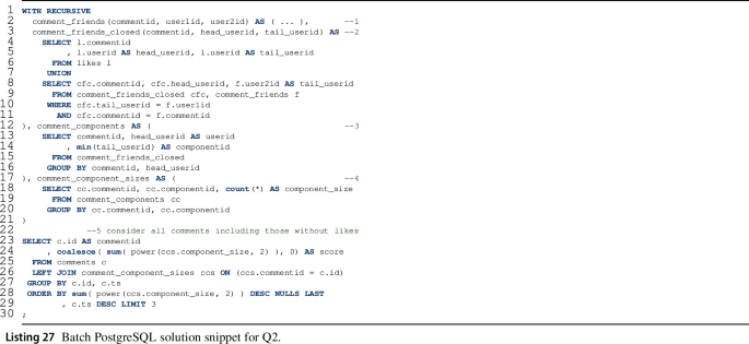
The outline of our Q2 implementation is shown in Listing 27. (The full query is given in Listing 30.) The implementation defines interim views using four subqueries and computes the result with the final (5th) query:

• 1. comment_friends(commentid, user1id, user2id): for a given $\textsf {Comment}$, pairs of $\textsf {User}$s who liked it and are friends.

• 2. comment_friends_closed(commentid, head_userid, tail_userid): the transitive closure of cf relations, i.e. for a given $\textsf {Comment}$, all pairs of $\textsf {User}$s who are reachable from each other through $\textsf {friends}$ edges.

• 3. connected_components(commentid, userid, componentid): for a given $\textsf {Comment}$, the $\textsf {User}$s who belong to a given component of the friendship graph.

• 4. comment_component_sizes(commentid, componentid, component_size): for a given $\textsf {Comment}$, the component IDs and their size.

• 5. Finally, the resulting relation contains the top-3 $\textsf {Comment}$s with the highest scores.

3.13 PostgreSQL incremental

To improve performance for repeated query executions, we have extended the PostgreSQL Batch solution (Sect. 3.12) with support for incremental updates. This section discusses the changes introduced in the schema and presents the queries that maintain the results upon changes.

3.13.1 Tool description

For the incremental solution, we have extended the database schema as shown in Fig. 7. Compared to the batch schema, this has three auxiliary relations and an extra attribute: (1) $\textit{q1}\_\textit{scoring}$ for maintaining the scores and timestamps of the $\textsf {Post}$s as defined in Q1, along with (2) $\textit{cf}$ and (3) $\textit{cfc}$ with the same semantics as in the Batch solution of Q2. The attribute (4) $\textit{comments.postid}$ is where Q1 maintains the root $\textsf {Post}$ reference for each $\textsf {Comment}$, which is then used in Q1. Additionally, we have employed a horizontal partitioning strategy [1] on each table. The partitioning uses an attribute status consisting of a single character “B” or “D”. During a particular update phase, rows that were already in the database are stored in the “B” (before) partition, while rows that have just been inserted are temporarily stored in the “D” (diff) partition. At the end of each update phase, rows from the diff partition migrate to the before partition. For both queries, we implemented algebraic incremental view maintenance with delta queries derived using the rules given in [38] and [81, Appendix E].

Fig. 7

ER diagram of the database schema, extended for incremental processing with 3 tables, 1 attribute to hold the root $\textsf {Post}$ reference of the $\textsf {Comment}$s and 5 status attributes added to the existing tables (highlighted in yellow boxes with dashed borders)

3.13.2 Query 1

The incremental solution for Q1 consists of three steps, each affecting the $\textit{q1}\_\textit{scoring}$ auxiliary relation, i.e. an initial step, then, for each update of the graph, a sequence of interim result maintenance and final result retrieval queries.

• 1. The initial step consists of two substeps:

  • (a) We compute the root $\textsf {Post}$ reference for all $\textsf {Comment}$s (Listing 31) and materialize in attribute $\textit{comments.postid}$.

  • (b) We compute the score for all $\textsf {Post}$s (Listing 32)—similarly to the batch solution of Q1 except that we materialize each $\textsf {Post}$ in relation $\textit{q1}\_\textit{scoring}$ with its timestamp and score.

• 2. The interim result maintenance is again split into two substeps:

  • (a) In preparation, we compute the root $\textsf {Post}$ reference for all new $\textsf {Comment}$s (Listing 33) and materialize in attribute $\textit{comments.postid}$.

  • (b) $\textsf {Post}$s ’ score maintenance (Listing 34) is implemented using three subqueries, each computing the increment in score for certain types of changes:

    • The $\textit{diff}\_\textit{posts}$ subquery calculates the score of the new $\textsf {Post}$s. The $\textsf {Comment}$s and likes of the new $\textsf {Post}$s must also be new, so the diff partition of all 3 relations are joined together. A left outer join is applied to include each new $\textsf {Post}$ regardless of whether it has received any $\textsf {Comment}$s and/or likes yet.

    • The $\textit{diff}\_\textit{comments}$ subquery calculates the extra score for old $\textsf {Post}$s gained by new $\textsf {Comment}$s and the likes for them. This is expressed as the inner join of the before partition of $\textsf {Post}$s and diff partition of $\textsf {Comment}$s. Then, a left outer join of the diff partition of likes is applied, as only new likes can refer to new $\textsf {Comment}$s, and we need to calculate scores of all new $\textsf {Comment}$s regardless of whether it received any likes.

    • The $\textit{diff}\_\textit{likes}$ subquery computes extra score for old $\textsf {Post}$s based for the new likes of their old $\textsf {Comment}$s. This is expressed as the inner join of the before partition of $\textsf {Post}$s and $\textsf {Comment}$s, and the diff partition of likes.

    In each subquery, one operand of the inner join is the diff partition of either the $\textit{posts}$, $\textit{comments}$ or $\textit{likes}$ relations. Their usually small record count can be exploited by the SQL query optimizer to speed up joins. Using the calculations above, $\textit{q1}\_\textit{scoring}$ is updated by increasing the scores of old $\textsf {Post}$s and inserting new $\textsf {Post}$s along with their scores.

    The relational algebraic formula for this interim result maintenance query is given in Fig. 13 and proved in Fig. 14.

• 3. The retrieval step is a simple top-3 query on $\textit{q1}\_\textit{scoring}$ (Listing 35).

3.13.3 Query 2

Similarly to Q1, the incremental solution for Q2 again consists of three steps, i.e. an initial step, then, for each update of the graph, an alternating sequence of interim result maintenance and final result retrieval queries. Both the initial and the maintenance steps are further divided into two queries affecting the $\textit{cf}$ and $\textit{cfc}$ interim relations.

• 1. During the initial step, we first compute the before partition of the $\textit{cf}$ relation (Listing 36), then its closure in the $\textit{cfc}$ relation (Listing 38). The queries to perform this are analogous to the corresponding subqueries of the PostgreSQL Batch solution for Q2 (Listing 27).

• 2. The maintenance step consists of two substeps:

  

  • (a) Updating the $\textit{cf}$ relation with a union of new $\textit{comment}\_{} \textit{friends}$ edges induced (Listing 37). Considering the $\textit{friends.user1id}$ as the left side on the join, and $\textit{friends.user2id}$ as its right side, a new edge is included by either:

    • i. the new likes on the left side of all friendships with all likes on the right side,

    • ii. the old likes on the left side of new friendships and all likes on the right side, and

    • iii. old likes on the left side of old friendships and new likes on the right side.

  • (b) Updating the transitive closure is done in three successive subqueries (denoted as

    

    in Listing 39):

    • i Each new like on a particular $\textsf {Comment}$ is a new zero-length path in the closure.

    • ii Instead of performing the computation on the $cf$ graph, we use new edges ($\textit{comment}\_\textit{friends}\_{} \textit{diff}$) to reach a fixed point in fewer steps.

    • iii The optimization in the previous step omitted the edges in the existing transitive closure, and hence, we add these to the result as a final step.

• 3. The retrieval step, similarly to the PostgreSQL Batch solution for Q2, computes the component sizes, and then, the scores for all $\textsf {Comment}$s are computed to retrieve the top-3 scored $\textsf {Comment}$s (Listing 40).

3.14 GraphBLAS Batch

Table 3 Notation of the GraphBLAS operations and methods used in this paper (based on [25])

3.14.1 Tool description

GraphBLAS is a recently proposed standard built on the theoretical framework of matrix operations on semirings [57], which allows concise and portable formulation of graph algorithms [58]. The goal of GraphBLAS is to create a layer of abstraction between the graph algorithms and the graph analytics framework, separating the concerns of the algorithm developers from those of the framework developers and hardware designers. The GraphBLAS standard defines a C API [20] that can be implemented on a variety of hardware components including GPUs.

Data format An untyped graph can be represented as an adjacency matrix $\mathbf {A} \in \mathbb {N}^{| V | \times | V |}$, where rows and columns both represent nodes of the graph and element $A_{ij}$ represents the number of edges from node i to node j. If the number of edges is not important, the adjacency matrix is defined over Boolean values, i.e. $\mathbf {A} \in \mathbb {B}^{| V | \times | V |}$, with $A_{ij} = 1$ if there is an edge from node i to node j and $A_{ij} = 0$ otherwise. Bipartite graphs can be represented with a non-square adjacency matrix $\mathbf {A} \in \mathbb {N}^{|V_1| \times |V_2|}$, where $V_1$ and $V_2$ are the sets of vertices in the two partitions. Typed graphs such as the ones used in this paper can be represented as using a bipartite adjacency matrix for each edge type, where $V_1$ represent the source nodes and $V_2$ represents the target nodes, e.g. $\mathbf {Likes} \in \mathbb {B}^{| users | \times | comments |}$. The graphs used in practical applications such as social networks are sparse. The adjacency matrices representing these graphs are also sparse, i.e. most elements in their adjacency matrix are zero values. These sparse matrices can be represented efficiently using matrix compression techniques such as CSR (Compressed Sparse Row).

A graph can also be stored as an incidence matrix $\mathbf {B} \in \mathbb {B}^{| V | \times | E |}$, where rows and columns represent nodes and edges (resp.). For undirected graphs, each column contains two 1 values in the positions of the source and the target nodes of the edge, and other elements are 0. Incidence matrices are sparse for all graphs with more than a few nodes.

Notation We follow the notation conventions of GraphBLAS as presented in [25]. Table 3 contains the list of GraphBLAS operations and methods used in this paper. Matrices are typeset in bold and start with an uppercase letter, e.g. $\mathbf {Friends}$. Vectors are typeset in bold and start with a lowercase letter, e.g. $\mathbf {scores}$. Additionally, sets are typeset in italic and start with a lowercase letter, e.g. $posts$.

Implementation For this solution, we used SuiteSparse:GraphBLAS  [25], a parallel GraphBLAS implementation and LAGraph  [64], a library of GraphBLAS algorithms. We also implemented an incremental solution in GraphBLAS, described in Sect. 3.15.

Fig. 8

Execution of the GraphBLAS algorithms on the example graph (Fig. 5): the Initial evaluation step (used by both the batch and incremental solutions) and the Update and re-evaluation step (used by the incremental solution). Recall that the update in the example inserts the following relevant entities (highlighted with grey background): a $\textsf {friends}$ edge between $\textsf {User}$s u1 and u4, a $\textsf {likes}$ edge from $\textsf {User}$ u2 to $\textsf {Comment}$ c2, a $\textsf {Comment}$ node c4 with a root $\textsf {Post}$ of p1 and an incoming $\textsf {likes}$ edge from $\textsf {User}$ u4

3.14.2 Query 1

Q1  (Algorithm 1) computes the score for each $\textsf {Post}$, then selects the top-3 $\textsf {Post}$s. We use an auxiliary $\mathbf {RootPost}$ $^\mathsf{T}$ adjacency matrix to denote the $\textsf {Post}$ a $\textsf {Comment}$ belongs to (possibly through a series of $\textsf {Comment}$s). The algorithm receives direct $\textsf {Comment}$s on $\textsf {Post}$s  ($\mathbf {CommentedP}$ $^\mathsf{T}$) and $\textsf {Comment}$s on other $\textsf {Comment}$s  ($\mathbf {CommentedC}$ $^\mathsf{T}$) separately. Starting from the former (Line 7), BFS is used to find child $\textsf {Comment}$s level by level and collect them to the $\textsf {Post}$ they belong to until there are no more left (Lines 8-10). In Line 12, the row-wise summation of $\mathbf {RootPost}$ $^\mathsf{T}$ matrix produces the number of (direct and indirect) $\textsf {Comment}$s per $\textsf {Post}$, and then, an ’apply’ operation multiplies the vector elements by 10. Line 14 sums up the number of likes the $\textsf {Post}$ has via its $\textsf {Comment}$s. For each $\textsf {Post}$, the $\mathbf {RootPost}$ $^\mathsf{T}$ adjacency matrix selects the elements of the $\mathbf {likesCount}$ vector corresponding to the $\textsf {Comment}$s of the $\textsf {Post}$ and then sums up the values. The score for each $\textsf {Post}$ is the element-wise sum of the two vectors (Line 15). Figure 8a shows an example calculation.

3.14.3 Query 2

A batch evaluation example of Q2  (Algorithm 2) is depicted in the upper part of Fig. 8b. Q2 computes the score for each $\textsf {Comment}$ and then selects the top-3 $\textsf {Comment}$s. To collect the $\textsf {User}$s of each subgraph, in Lines 8 and 10, extracts the elements of the $\mathbf {Likes}$ $^\mathsf{T}$ matrix as $( c, u, 1 )$ tuples and collects them into sets of $\textsf {User}$ IDs (u) per $\textsf {Comment}$  (c). To produce the subgraph for each $\textsf {Comment}$, extracts a submatrix based on the $\textsf {User}$s selected (Line 11). finds connected components in the induced subgraph using the FastSV algorithm [88] of the LAGraph library (Line 12). This produces a vector containing the component ID for each $\textsf {User}$. yields the squared sum of component sizes, i.e. the score for each $\textsf {Comment}$  (Line 14).

3.15 GraphBLAS incremental

3.15.1 Tool description

To incrementalize the GraphBLAS Batch solution (Sect. 3.14), we have reworked the solution to compute changes to the results upon updates instead of running a full re-evaluation.

Approach The incremental version performs a full batch evaluation for the first run and computes the scores. Then, for each update only those parts of the model are re-evaluated which might be affected by the update. Finally, the previous top-3 scores and the new ones are compared to maintain the result. Incremental computation of Q1 uses fine-grained maintenance as it stores the scores of each $\textsf {Post}$ and updates them when new $\textsf {Comment}$ nodes and $\textsf {likes}$ edges appear. The granularity of the incremental version of Q2 is coarser, as it collects the $\textsf {Comment}$s whose scores can change and re-evaluates them.

Notation The updated variables are denoted with prime, e.g. the updated version of vector $\mathbf {scores}$ is $\mathbf {scores'}$, which contains the scores for the new nodes and the updated scores for the existing ones. The changes can be stored as increment matrices/vectors, denoted with a superscript plus symbol ($\mathbf {^+}$) and are applied with the $\oplus$ operation to the original values, e.g. ${ \mathbf {scores'} = \mathbf {scores} \oplus \mathbf {scores^+} }$. Another option is to store the changed values, denoted with ${\Delta }$, and apply them by overwriting the existing values: the new vector is initialized with the original one: ${ \mathbf {scores'} = \mathbf {scores} }$, then the new values overwrite the existing ones via a mask, which preserves the unaffected values from modification: ${ \mathbf {scores'} \langle \!\langle {\Delta }\mathbf {scores} \rangle \!\rangle = {\Delta }\mathbf {scores} }$.

3.15.2 Query 1

To incrementally evaluate Q1, Algorithm 3 updates the scores as follows. Lines 9 and 10 compute the increment of the score induced by new $\textsf {Comment}$s. In Line 11, the number of likes the $\textsf {Comment}$s newly received is summed up per $\textsf {Post}$. The two types of increments are summed up in Line 12. For subsequent evaluations, the scores are updated using the increment vector (Line 13). To find the top-3 scores, only the previous maximum values and the $\textsf {Post}$s with updated scores are considered. Line 14 yields the updated score values by assigning the $\mathbf {scores'}$ vector via the $\mathbf {scores^+}$ increment vector as a mask, which allows changes in the result only if the mask has an element at the corresponding position. Figure 8a shows an example calculation. Using the output of this algorithm, merging the previous top-3 scores and the new ones yields the new result.¹³

3.15.3 Query 2

The incremental evaluation of Q2 is depicted in the lower part of Fig. 8b. Algorithm 4 returns the $\textsf {Comment}$s with new scores (${\Delta }\mathbf {scores}$) by re-evaluating the $\textsf {Comment}$s which the updates might impact on. Merging the previous top-3 scores and the new ones yields the new result. (New scores overwrite existing ones.) The first phase of the algorithm (Steps  – , Lines 14–20) collects the $\textsf {Comment}$s which might be affected by the updates (affected comments, $acSet$ set), and then, the second phase (Steps  – , Line 21) computes the new scores of these $\textsf {Comment}$s using the batch algorithm described in Algorithm 2.

A $\textsf {Comment}$ might be affected by an update if (1) it is a new $\textsf {Comment}$, or (2) the $\textsf {Comment}$ receives a new incoming $\textsf {likes}$ edge from a $\textsf {User}$, resulting in a new component or the expansion of an existing one, or (3) two $\textsf {User}$s who like the $\textsf {Comment}$ become friends, which merges the components the $\textsf {User}$s belong to (if they previously belonged to different components). Case (3) is covered by Lines 14-18, where Steps  – compute the $\textsf {Comment}$s which might be affected by new $\textsf {friends}$ edges. $\mathbf {NewFriends}$ incidence matrix represents each new friendship by a column having two 1-/valued elements for the two $\textsf {User}$s. For each new friendship (i.e. pair of $\textsf {User}$s), computes how many $\textsf {User}$ of the pair likes each $\textsf {Comment}$  ($0, 1, \text {or } 2$). During the matrix–matrix multiplication, each column of new friendships selects two columns of $\mathbf {Likes'}$ $^\mathsf{T}$ matrix and sums them up into $\mathbf {AC}$ matrix (Line 15). In Line 16, keeps only 2-/valued elements, i.e. where both $\textsf {User}$s of a friendship liked the $\textsf {Comment}$, so both of them are present in the subgraph and the new friendship might merge components. Then, produces a row-wise sum using the logical or operator $\vee$ (Line 17). extracts $( c, 1 )$ tuples from the result vector and collects the $\textsf {Comment}$ IDs from these tuples, then collects all the $\textsf {Comment}$s which might be affected by the update (Line 19). Cases (1) and (2) are covered by Line 20, which produces the union of all the three cases. The next steps re-evaluate the scores of these $\textsf {Comment}$s  (Line 21).

3.16 Differential dataflow

3.16.1 Tool description

Dataflow-based computational models were proposed to perform complex analytics on high-volume data sets: the timely dataflow [69, 70] model targets batch processing, while its extension, differential dataflow [65], targets incremental processing.

We created two differential dataflow-based solutions:

.NET-based implementation Naiad¹⁴ is a data processing prototype system developed at Microsoft Research¹⁵ between 2011 and 2014. Naiad supports both the timely and differential dataflow computational models. The Naiad implementation was written in C#.

Rust-based implementation The computational models of Naiad have been implemented in the Rust programming language¹⁶ [59] as two separate projects: Timely Dataflow¹⁷ and Differential Dataflow.¹⁸

For the sake of brevity, we only discuss the Rust-based implementation here—the one using Naiad is available online but has been omitted from this paper.

Data representation To represent the graph, the Differential Dataflow solution uses unordered collections containing tuples with the following semantics:

• comms: (id, ts, content, creator, parent)

• posts: (id, ts, content, creator)

• knows: (user1, user2)

• likes: (user, comment)

3.16.2 Query 1

The implementation of Q1 (shown in Listing 28) uses the comms, posts, and likes collections. In Line 8, we extract the $\textsf {Comment}$s and their direct parent objects, which can either be a $\textsf {Post}$ or another $\textsf {Comment}$. In Lines 19–13, we determine the direct replies for each $\textsf {Post}$. Next, in Lines 14–25, we collect all transitive replies for each $\textsf {Post}$ using the iterate operator, which executes the specified function until a stable result set is reached. In Lines 26–31, we collect the number of $\textsf {likes}$ for each $\textsf {Comment}$, each having a cardinality of 1 (corresponding to their contribution to the overall score). Then, in Line 32, we collect each $\textsf {Comment}$ that belongs to the $\textsf {Post}$ with a cardinality of 10 (as they are worth 10 points). Next, in Lines 33–38, we concatenate the collections containing the likes and the reply $\textsf {Comment}$s and count their total cardinality. Finally, in Lines 39–41, we add the timestamps of each $\textsf {Post}$ and get the top-3 values.

3.16.3 Query 2

The implementation of Q2 (shown in Listing 29) uses the comms, knows and likes collections. First, in Lines 8–25, we use iterative label propagation to find connected components. Initially, we add the labels based on the likes edges and then propagate them across the knows edges. When the propagation reaches its fixed point, we will have a list of (user, label, comment) tuples, where each tuple shows that the given $\textsf {User}$ is part of the connected component of the given $\textsf {Comment}$, and the smallest $\textsf {User}$ id in this connected is the label. Then, in Lines 26–35, we aggregate the labels to get the size of each connected component and get the final score by summing the squared component sizes. Finally, we add the timestamps of each $\textsf {Comment}$ and get the top-3 values.

4 Classification

In this section, we compare the solutions according to our predefined classification criteria, evaluating general tool properties as well as case-specific applications of them. Aligned with the research questions, we used the following classification criteria:

• Declarative query language To aid the development of the solutions using the respective tools, it is helpful for the tool to adhere to a standard declarative query language.

• Data model For a usage integrated into a modelling tool set, ideally model query tools should be able to use models created and maintained in a modelling environment as they are, without adapters.

• Explicitness of incrementalization Ideally, tools are able to incrementalize the query in an implicit manner, i.e. the developer only has to specify the query, but not how changes are propagated or how the query is broken down into chunks. This criterion does not apply to batch solutions, i.e. ones that recalculate the query from scratch after each model change.

• Persistence To enable a failsafe operation, it is a desirable property for an analysis tool to continue the analysis even if the process is unexpectedly shut down. For this, data structures to save intermediate results have to be persisted, which is why we call this category query persistence. Further, in order to process models beyond the size of the main memory, it is desirable to persist the models in a database such that solutions do not have to have all model elements in memory. We refer to this as model persistence.

• Parallelism As modern CPUs have multiple cores, it is desirable for a query technology to be able to make use of these resources by running parts of the query or its incremental change propagation in parallel.

• Asymptotic complexity to propagate changes We present an estimated asymptotic complexity of the steps required to propagate changes. For this, we consider the necessary steps to propagate changes to both queries for all of the five possible changes (Sect. 2.3). The derived complexity values are specific to the particular scenario of the Social Media benchmark and thus should not be interpreted as a generic characterization of the tools.

In the following sections, we discuss the criteria for each of the solutions individually and summarize the results afterwards in Table 4, except for the asymptotic complexities that are depicted in Tables 5 and 6.

Table 4 Comparison of the tools used in the paper

Table 5 Asymptotic complexities to propagate a model update for Q1 in selected solutions

Table 6 Asymptotic complexities to propagate a model update for Q2 in selected solutions

4.1 Declarative query language

NMF makes use of the SQO (Standard Query Operators), which is a common standard on the .NET platform. Similarly, the Xtend solution uses the standard collection operators of Java. ATL uses (a slightly adapted version of) OCL. The SQL and Neo4j solutions use the standard query languages of these databases: SQL:1999 and Cypher.

EOL used by Hawk is standard in Epsilon, but the community of Epsilon is much smaller than the community of relational databases, .NET or Neo4j.

AOF and YAMTL have their tool-specific query languages which are declarative (both solutions can be executed incrementally from the query specification) but not yet standards.

JastAdd uses its own language to specify synthesized and inherited attributes with tool-specific extensions like circular rules.

4.2 Data model

Given that the benchmark was originally presented at the TTC, it is not surprising that most solutions can operate directly on EMF models.

NMF uses its own metamodel NMeta but includes a transformation from Ecore and uses the same serialization format [45].

For JastAdd, it is necessary to reformulate the metamodel as grammar.

The solutions for Differential Dataflow, Neo4j, GraphBLAS and PostgreSQL do not operate on models directly but require dedicated adapters to feed the data from models into their input formats (CSV files).

4.3 Explicitness of incrementalization

The NMF reference solution, the ATL solution, the Xtend solution and the batch versions of SQL, Neo4j and GraphBLAS solutions are not incremental.

The incrementalization in the incremental NMF solution and in the AOF solution is implicit: the framework deducts a dependency graph from a model of the code that is available at runtime. This dependency graph is at the level of individual operations, so that only those operations really affected by a change need to be re-computed. However, these frameworks require data structures that explicitly support incrementalization. Both NMF and AOF already contain support for a wide range of common operations and allow $\textsf {User}$s to add new algorithms and data structures when needed, such as for calculating the connected components in Q2.

In the Hawk solutions, there are two aspects to incrementalization: the way that the persistent graph is updated and the way that the query is run. The batch solution uses derived attributes to cache the scores of $\textsf {Comment}$s and $\textsf {Post}$s, which are implicitly updated incrementally if the nodes used to compute them change: however, the queries run in batch mode, and every change in the social network requires a full re-serialization to disk before the indexing process can update the graph. The incremental update solution uses the same approach for querying, but it does not re-serialize the social network model: instead, it applies the change sequences directly to the internal graph used for querying. The incremental update and query solution uses an explicitly incrementalized version of the query, using graph listeners to trigger the rescoring of $\textsf {Comment}$s and $\textsf {Post}$s, and uses the same approach to directly update the underlying graph database from the NMF change sequences.

JastAdd and YAMTL support a completely implicit incrementalization by tracking all read operations to the model from which a dependency graph is set up. If the result of a rule depends on a read operation that is invalidated due to model changes, this attribute instance (JastAdd) or rule instance (YAMTL) is executed again. Therefore, the granularity of the incrementalization is given by the granularity of the attributes/rules.¹⁹

In the incremental versions of the SQL, Neo4j and GraphBLAS solutions, the incrementality is achieved explicitly. That is, these solutions all keep the scores of $\textsf {Post}$s or $\textsf {Comment}$s through a table, additional nodes or vectors, respectively. Then, the solutions use explicit algorithms developed for the respective tool to update the scores in case of model updates.

In case of the SQL solution, this effort to explicitly reengineer existing queries for incremental change propagation is guided [38, 81]. Such guidance can help the developer incrementalize a given query and could be automated when sufficient tooling becomes available.

The Differential Dataflow solution works similar to NMF and AOF. However, the notion of time during the calculation of the query allows this tools to support temporary state, in particular the iterate call in Listing 29. This temporary state allows to support also more complex cases such as computing connected components in Q2 using only built-in algorithms and data structures [70].

In total, we have nine non-incremental solutions. PostgreSQL, Neo4j, YAMTL-EI and GraphBLAS are explicitly incrementalized, so developers have to approach the problem conceptually differently than in the batch solution. Hawk provides slight implicit incrementalization capabilities, but much of the solution must be provided by the developer in order to get the solution incremental; therefore, we categorized it as an explicit incremental tool. In NMF, JastAdd, AOF, YAMTL-II, Incremental ATL Incremental and Differential Dataflow, the incrementalization happens entirely implicitly, though partially with restrictions. Namely, JastAdd and YAMTL require the developer to adapt to their programming model, whereas NMF and AOF restrict the used operations to those that are supported in the framework, even if this set is extensible. Differential Dataflow does not have such restrictions.

4.4 Persistence

Most of the presented solutions keep the data only in memory without any features for fault-tolerance. This means that the solutions require a separate tooling to ensure a failsafe operation.

The exceptions to this are Hawk, Neo4j and PostgreSQL, which make use of database systems internally and are therefore durable, in the sense that models and intermediate query results for their incremental variants are available even if the application gets terminated unexpectedly.

For many of the other tools, model persistence could be achieved through persistence systems such as Eclipse CDO.²⁰ However, although the model sizes used in the scope of the benchmark went up to a few million model elements and connections, solutions were always able to handle the models in main memory. Therefore, the need for solutions with model persistence to hit the disk for an update led to performance penalties in comparison with other solutions.

The advantage that Hawk and the incremental versions of Neo4j and PostgreSQL take out of the persistence of the intermediate results is that after a restart, they do not require the performance penalty of an initial run again and can process updates straight away after a restart. The exception to that is the incremental update and query solution for Hawk, since this keeps an in-memory list of the top-3 elements.

4.5 Parallelism

Since GraphBLAS is based on matrix operations, it is well suited for parallel processing. Differential Dataflow also supports executing the query in parallel. The Xtend solution makes use of the Java streams feature to enable parallelism, but only on a task level, i.e. the solution runs different parts of the query in a pipeline.

NMF also has some built-in support for parallelism, but it is restricted only to the incremental change propagation. The initial query execution does not profit from the parallel execution.

The other solutions do not make use of parallelism.

4.6 Asymptotic complexity to propagate changes

Recall that in Sect. 2.3, the following change operations were presented: (1) a new $\textsf {User}$ is added, (2) a new $\textsf {Post}$ is added, (3) a new $\textsf {Comment}$ is added to an existing $\textsf {Post}$, (4) a $\textsf {Comment}$ is liked, and (5) two existing $\textsf {User}$s become friends.

In the remainder of this section, we denote the number of $\textsf {User}$s in a model with u, the number of $\textsf {Post}$s with p, the number of $\textsf {Comment}$s with c and the number of likes with l. A $\textsf {Post}$ may have up to n $\textsf {Comment}$s including transitive replies. The maximum hierarchy depth of $\textsf {Comment}$s is denoted by h. A group of $\textsf {User}$s that like the same $\textsf {Comment}$ and are connected through friendships has the maximum size f.

4.6.1 NMF Batch, Xtend, ATL

The NMF reference solution and the ATL solution are batch implementations where all changes result in a complete recalculation of the analysis. For Q1, calculating the scores of each $\textsf {Post}$ takes $\varTheta (p+c)$ time, plus $\varTheta (p \log p)$ for the sorting. This amounts to $\varTheta (p \log p + c)$. For Q2, Tarjan’s algorithm or a similar algorithm to obtain connected components is executed for each $\textsf {Comment}$. Tarjan’s algorithm has a linear complexity in both nodes and edges where there are at most $f^2$ edges, leading to a complexity of $O(c \cdot f^2)$. However, because $\textsf {User}$s only need to be considered for $\textsf {Comment}$s they have liked and every like corresponds to exactly one node in the induced graph for the liked $\textsf {Comment}$, this can be reduced to $O(l \cdot f)$. Together with $O(c \log c)$ for sorting the $\textsf {Comment}$s, this leads to $O(l \cdot f + c \log c)$ for Q2. For Xtend, the sorting step is avoided by a dedicated stream operator in both queries. Furthermore, the usage of streams in the Xtend solution theoretically allows to calculate the scores of the individual $\textsf {Comment}$s or $\textsf {Post}$s in parallel.

4.6.2 NMF incremental, AOF, ATL incremental, differential dataflow

In the incremental NMF solution as well as in the AOF, incremental ATL and Differential Dataflow solutions, the analysis is slightly more complex. Adding a new $\textsf {User}$ does not touch the dependency graph for Q1, and thus, the effort for change propagation is constant, same for the change that two $\textsf {User}$s become friends. When a new $\textsf {Post}$ is added, it does not have any $\textsf {Comment}$s, but has to be inserted in the binary search tree of $\textsf {Post}$s. This has an effort of $O(\log p)$. Adding a new $\textsf {Comment}$ will ripple through the Descendants or AllInstances operation and cause an effort of O(h), followed by $\varTheta (\log p)$ to update the position of the $\textsf {Post}$ in the binary search tree. When a $\textsf {Comment}$ is liked, this only causes constant effort to update the sum, but O(h) to find the corresponding $\textsf {Post}$ and $\varTheta (\log p)$ to update the position in the search tree.

For Q2, the insertion of a new $\textsf {User}$ does not touch the dependency graph because the new $\textsf {User}$ does not have friends and has not liked any $\textsf {Comment}$s yet. Similarly, the insertion of a $\textsf {Post}$ only causes constant effort to the change propagation. The insertion of a $\textsf {Comment}$ only requires to calculate connected components of an empty graph (the $\textsf {Comment}$ is not liked, yet) and inserting it into the binary search tree, which takes $O(\log c)$. Liking a $\textsf {Comment}$ requires to re-compute the connected components for this $\textsf {Comment}$ and updating the score in the search tree, which is $O(f^2 + \log c)$ since the connected components are computed from scratch. If two $\textsf {User}$s become friends, this potentially changes the subgraphs for all $\textsf {Comment}$s, which has a complexity of $O(l \cdot f + c \log c)$ just as if we were to recalculate the entire query, though in the average case, many new friendships will likely not affect all $\textsf {Comment}$s.

The parallel execution of NMF and Differential Dataflow does not change the complexity to perform a change, and it is rather used to propagate the changes within the transaction in parallel.

4.6.3 Hawk

In Hawk, the batch update process needs to check the entire model for changes, which clearly is $\varOmega (p+c+u \cdot f)$. For incremental updates, the time to perform the graph updates is constant. However, in both cases, the indices need to be re-computed. For Q1, this takes $\varTheta (n)$ time plus $O(p \log p)$ for sorting the $\textsf {Post}$s as soon as the score for a $\textsf {Post}$ needs to be re-computed, i.e. when adding or liking a $\textsf {Comment}$. The incremental query eliminates the sorting step, explicitly taking advantage of the monotony of the scores in this scenario.

For Q2, similarly to the incremental NMF and AOF solutions, the insertion of a $\textsf {User}$ or a $\textsf {Post}$ does not have any effect because they do not invalidate the score of any $\textsf {Comment}$. However, the solution still requires the sorting, which takes $O(c \log c)$, unless the solution is run in the incremental query mode (in which case the sorting is replaced by constant effort, using the monotony of the scores). If a $\textsf {Comment}$ is liked, the calculation of connected components is invalidated and recalculated for this $\textsf {Comment}$, which takes $O(f^2)$. A new friendship requires the score of all $\textsf {Comment}$s to be re-evaluated, which is complexity of $O(l \cdot f)$.

4.6.4 JastAdd

JastAdd tracks accesses to model elements when an attribute (score) of a model element is computed and uses this to invalidate these attributes upon a model change. However, the maximum always has to be computed. Adding a new $\textsf {User}$ or two $\textsf {User}$s becoming friends in Q1 (changes that do not affect any model feature used in computing the scores) has a complexity of $\varTheta (p)$. This complexity also dominates the score calculation for a new $\textsf {Post}$ (without $\textsf {Comment}$s). Adding or liking a $\textsf {Comment}$ will invalidate the score for the $\textsf {Post}$ and cause JastAdd to re-compute the score for this $\textsf {Post}$, which requires a complexity of O(n) in addition to the $\varTheta (p)$.

For Q2, finding the maximum takes $\varTheta (c)$ and for inserting a $\textsf {User}$ or $\textsf {Post}$, that is the overall complexity because the new $\textsf {User}$ or $\textsf {Post}$ is not being read in any score calculation. A new $\textsf {Comment}$ only requires to calculate the score for that $\textsf {Comment}$ in addition, which takes only constant effort. Liking a $\textsf {Comment}$ will invalidate the score for this $\textsf {Comment}$, which again takes $O(f^2)$ and a new friendship takes $O(l \cdot f)$ as this friendship may affect the score for many $\textsf {Comment}$s.

4.6.5 YAMTL

In the YAMTL solutions, only the three best candidates are retained and this simplifies the sorting step, which becomes constant. Discarding a candidate has constant time, and when the candidate is valid, it takes up to two comparisons to update the list.

In Q1, YAMTL-B calculates the scores by traversing all $\textsf {Post}$s and then all of their $\textsf {Comment}$s, $O(p+c)$. When adding $\textsf {Comment}$s or likes, YAMTL-II re-computes the score for each matched $\textsf {Post}$ affected by a change, traversing all of its contained $\textsf {Comment}$s, O(n). Instead, YAMTL-EI only processes the new $\textsf {Comment}$ that has been added to the $\textsf {Post}$ or that has been liked by another $\textsf {User}$ for each impacted $\textsf {Post}$, so the update is O(1) in those cases.

In Q2, for each $\textsf {Comment}$, Sedgewick and Wayne’s weighted quick union find with path compression initializes components in linear time, $O(l \cdot f)$, where the initial size of components is given by l. Find and union operations have an amortized cost that corresponds to the inverse of Ackermann’s function, $O(\alpha (l))$. YAMTL solutions match $\textsf {Comment}$s instead of $\textsf {Post}$s in Q2. For computing a $\textsf {Comment}$ score, YAMTL’s solution applies the union operation for any friend that has liked the $\textsf {Comment}$, so processing each $\textsf {Comment}$ involves $O(l \cdot f \cdot \alpha (l))$. In propagation mode, YAMTL-B initializes the data structures for the weighted quick union find with path compression for $\textsf {User}$s l in each $\textsf {Comment}$, and the cost is $O(l \cdot f \cdot \alpha (l) + c)$. YAMTL-II visits the $\textsf {Comment}$s affected by changes and initializes the connected components of friends from scratch, so the cost is $O(l \cdot f \cdot \alpha (l))$ when adding a like and when adding a friendship. YAMTL-EI is sensitive to finer changes, adding a like by a new $\textsf {User}$ triggers the update of connected components with the friends f of the new $\textsf {User}$, $O(f \cdot \alpha (l))$, whereas a new friendship only involves computing the union of two components, $O(\alpha (l)).$

4.6.6 PostgreSQL batch

Compared to solutions working on object models, an RDBMS has the problem that references to other models are not directly available as object references but usually lead to an indirect reference that must be resolved using an index. The choice of this index and also the exact query strategy is generally specific to the RDBMS and may differ from our estimation here. In the remainder, we assume search trees are used that resolve such a reference in log time. This allows to manage data beyond main memory limitations but is of course slower than following a direct reference.

For Q1, the root $\textsf {Post}$ reference for each $\textsf {Comment}$ is computed first in $\varOmega (c \cdot \log c)$, which stands for the cost of the first self-join of $\textsf {Comment}$s when computing the transitive closure. Then $\textsf {Post}$s are outer joined with their $\textsf {Comment}$s in $\varOmega (p \cdot \log c + p + c)$ steps to produce an interim result size proportional to $p + c$, which is then outer joined with their likes in $\varOmega (\left( p + c\right) \cdot \log l + p + c + l)$ and the count of likes has to be computed in $\varOmega (l)$ steps. In-memory solutions, by contrast, can easily read the count as it is usually directly available for array list implementations of collections. Thus, the batch implementation has a complexity of $\varOmega (c \cdot \log c + p \cdot \log c + \left( p + c\right) \cdot \log l + p + c + l)$, which can be further simplified to $\varOmega ( \left( p + c\right) \cdot \log cl + l)$.²¹

In Q2, we first compute the transitive closure of the friendship subgraphs²² in $\varOmega (l \cdot \log lfl + l + f + l)$, which stands for the cost of the first recursive step. The size of the transitive closure is $\varOmega (l)$, which is fed as input to the subsequent aggregations that can be done in linear time w.r.t. their input size. The result of the aggregations has again a size of $\varOmega (l)$, and as it exists only in memory, no index is available. Thus, the final join to $\textsf {Comment}$s is assumed to be done using hash join with a complexity of $\varOmega (c + l)$. Summing up the former gives the batch implementation a complexity of $\varOmega (l \cdot \log lfl + l + f + l + l + c + l)$, which can be simplified to $\varOmega (l \cdot \log lf + l)$.²³

4.6.7 PostgreSQL incremental

For Q1, any score update of a $\textsf {Post}$ in the incremental SQL solution yields a complexity of $\varTheta (\log p)$. However, adding a new $\textsf {User}$ or friendship does not cause a score update and has therefore constant effort. Apart from that, adding a $\textsf {Post}$ only requires to left join an empty table with constant effort and migrating the $\textsf {Post}$ to the new partition, which we assume is constant effort. Adding a $\textsf {Comment}$ requires to resolve its $\textsf {Post}$ with a complexity of $\varTheta (\log p + \log c)$, adding a like causes $\varTheta (\log p \cdot \log c)$. For Q2, the result-retrieval is non-trivial even in the presence of an index and has an effort of $\varOmega (l \cdot f)$. Adding a $\textsf {User}$, $\textsf {Post}$ or $\textsf {Comment}$ changes neither friends nor likes relations, which is why all join operations to update the comment_friends relation in stages 0 and 1 inner join an empty table and thus become constant in the maintenance phase. Computing stage 2 and inserting into the comment_friends relation require to process all $O(c^2 f^2)$ entries of stage 2. Liking a $\textsf {Comment}$ or a new friendships adds an overhead to the computation of stage 1 and stage 2 (possibly recursively), but we assume this effort to be dominated by $O(c^2 f^2)$.

4.6.8 Neo4j incremental

The Neo4j solution saves the score as a property on $\textsf {Post}$ and $\textsf {Comment}$ nodes and indexes these properties using B-trees.²⁴ For Q1, this implies that inserting a new $\textsf {Post}$ necessitates a cost of $O(\log p)$ (maintaining the index on the $\textsf {score}$ property). Adding a $\textsf {Comment}$ or a like can result in an increase of the score of the root $\textsf {Post}$, which costs O(h) for finding the $\textsf {Post}$ and $O(\log p)$ to update the score. For Q2, the incremental solution materializes each $\textsf {Comment}$ ’s connected components which need to be maintained upon inserting a new likes edge. The non-trivial operations are as follows. When a $\textsf {Comment}$ is initially inserted, it has a $\textsf {score}$ of 0. Maintaining the index on the $\textsf {score}$ property incurs a cost of $O(\log c)$. When a $\textsf {User}$  $\textsf {usr}$ adds a new like to $\textsf {Comment}$  $\textsf {cmt}$, the solution merges all connected components of $\textsf {cmt}$ containing friends of $\textsf {usr}$ with a cost of $O(u \cdot f)$. Additionally, maintaining the index on the $\textsf {score}$ property of the $\textsf {Comment}$s has $O(\log c)$ cost. Finally, adding a new $\textsf {friends}$ edge necessitates checking which components of which $\textsf {Comment}$s can be merged, incurring a cost of $O(c^2)$ and maintaining the index for cost $O(\log c)$.

Apart from this, since Neo4j indexes store identifiers of nodes in search trees and checks uniqueness constraints, adding a $\textsf {User}$ requires an effort of $\varTheta (\log u)$, adding a $\textsf {Post}$ $\varTheta (\log p)$ and adding a $\textsf {Comment}$ $\varTheta (\log c)$. Liking a $\textsf {Comment}$ requires at least $\varTheta (\log u + \log c)$ and $\textsf {User}$s becoming friends at least $\varTheta (\log u)$ cost.

Table 7 Model sizes for each scale factor: number of nodes and edges, number of changes

4.6.9 GraphBLAS

For GraphBLAS, stating algorithmic complexities for query calculation is difficult because the engine automatically chooses from a variety of algorithms for matrix multiplication given that the matrices are usually very sparse. For example, the adjacency matrix to calculate the $\textsf {Comment}$s of a root $\textsf {Post}$ in the Q1 batch version is sparse because $\textsf {Comment}$s only belong to one root $\textsf {Post}$. A naïve implementation of calculating this sum would therefore take an effort of $O(p \cdot c)$, but this analysis does not take into account the optimizations that GraphBLAS applies to this computation. Therefore, we do not provide results for asymptotic complexity for GraphBLAS.

4.6.10 Summary

The asymptotic complexities for Q1 are summarized in Table 5. The table is divided into solutions that are not incremental at all at the top (including non-incremental executions of tools that are able to implicitly incrementalize the query), those that are implicitly incremental and derive the algorithm to propagate incremental changes from a declarative specification in the middle, and explicitly incremental solutions at the bottom.

One can see in Table 5 that whereas the non-incremental tools have a linear complexity with respect to the number of $\textsf {Post}$s and $\textsf {Comment}$s, many incremental tools have a better asymptotic complexity and therefore should scale much better in presence of changes as they have constant or logarithmic update efforts. However, there is a notable difference between NMF and AOF, which take a rather fine-grained approach to incremental change propagation, compared to JastAdd, Hawk and YAMTL that rely on chunks in the form of (derived) attribute or rule calculations. While the latter can speed up recalculation to constant times in some cases, the former approaches can get down to logarithmic efforts even when $\textsf {Comment}$s are added or liked as they allow partial recalculation of the score of a $\textsf {Comment}$. These complexities also could be beaten by solutions where the incremental change propagation is explicitly specified by the developer, at least using the approaches studied.

The results for asymptotic complexities for Q2 are summarized in Table 6. The solutions are ordered in the same way as in Table 5. While for adding $\textsf {User}$s, $\textsf {Post}$s or $\textsf {Comment}$s, the results look very similar to Q1 with incremental approaches achieving a strictly better asymptotic complexity, the results for liking a $\textsf {Comment}$ or especially $\textsf {User}$s becoming friends are not as good. This is partially because the analysis of asymptotic complexities is not very detailed,²⁵ but it is also a consequence of the effect that these changes simply have a large impact on the computations that get invalidated. A new friendship changes the connected components in the induced subgraphs of the $\textsf {Comment}$s that both $\textsf {User}$s have liked.

5 Performance evaluation

In this section, we present the results of the performance measurements with respect to the time required to load the models, to run the initial query evaluation, and to propagate changes. We first present the benchmark setup and experiment design and then analyse the results. Finally, we discuss potential threats to validity.

5.1 Benchmark setup

5.1.1 Input models

We executed the benchmark on models of increasing sizes, denoted by scale factors (SFs) of power of 2. The number of elements per node/edge type in each SF is shown in Table 7. The largest model has 0.86M nodes and 2.25M edges. The number of changes varies between 45 and 132 model elements.

5.1.2 Benchmark framework

The benchmark framework is based on the one of the TTC 2017 Smart Grid case [48] and supports automated build and execution of solutions as well as a correctness check and visualization of the results using R. The correctness is checked by comparing the query result against a pre-computed reference both after the initial transformation and after each update. The source code and documentation of the benchmark as well as metamodels, solutions, input models and change sequences used for benchmarking are publicly available online.²⁶ The benchmark repository also contains instructions on how to run the benchmark in Docker containers and there are Docker images of all solutions available in Docker Hub.²⁷

5.1.3 Benchmark environment

We ran the solutions on a cloud virtual machine with 8 cores of an Intel^® Xeon^® Platinum 8167M CPU, a base clock speed of 2.0 GHz and a turbo clock speed of 2.4 GHz. Hyper-Threading was turned off. The machine was running the Ubuntu 20.04.2 LTS operating system. To help reproducibility, the experiments were executed in containers managed by Docker 20.10.6. The runtime environments for Java- and .NET-based solutions were OpenJDK 1.8.0 update 282, OpenJDK 11.0.10 and .NET Core 3.1.14. Each tool was measured 5 times, and the geometric mean of the results is used. The timeout value for each run was set to 10 minutes.

The modelling tools used XML-based representations (e.g. XMI files) to load the data and the change set sequences. For the rest of the tools (Neo4j, GraphBLAS, PostgreSQL and Differential Dataflow), both the initial model and the change sequences were loaded from CSV files.

Fig. 9

Execution times of solutions with batch evaluation

5.2 Analysis

We grouped execution times by query, tool family and phase. To save space, we do not show the exact results, but these can be obtained from the GitHub repository of the benchmark. From the phases listed in Sect. 2.4, we omitted the initialization phase and kept the other three, i.e. (1) loading the models, (2) the initial run and (3) the time to apply a set of changes and update the result accordingly. In the following, we compare the solutions across tool boundaries. For each family of solutions, we only include the results for the best variant. A comparison of the solution variants for NMF, Hawk, JastAdd and YAMTL can be found in the appendix.

5.2.1 Batch solutions

The results for all batch tools are depicted in Fig. 9. One can immediately see that most lines in all of these diagrams have approximately the same slope. This confirms that query execution times grow approximately linearly with the size of the models.

The results for the initial execution times and the times to update the graph are also very similar. This is clear, given that after changing the model, the batch solutions all evaluate the entire query again. Particularly for small models, there is an overhead attached with the first execution, which is why the execution times for updates are slightly smaller. This overhead differs between the tools and is constant, thus hard to perceive on a log scale.

For the update times, one can see clear distances between the graphs, especially for Q1 where plotted execution times appear almost parallel, indicating constant factors, i.e. the solutions have different execution speeds but very similar scalability characteristics. The GraphBLAS batch solution outperforms all other batch solutions by more than one order of magnitude. JastAdd and YAMTL that come next are still faster than NMF by a factor of 3 and faster than the remaining by at least an order of magnitude for Q1.

For Q2, many solutions had severe performance problems which is why they did not complete for larger model sizes. One can also see that in particular for the SQL solution and the JastAdd solution, the slope is steeper for the larger model sizes, indicating the chosen algorithm implementation does not scale equally well.

For Hawk, one can see how the choice of the underlying database implementation affects performance: the performance using SQLite is mostly better, which is clear given that the entire models for all sizes fit into main memory.

Fig. 10

Execution times of solutions with implicit incremental evaluation

Fig. 11

Execution times of solutions with explicit incremental evaluation

5.2.2 Implicit incremental solutions

For the implicitly incremental solutions, the results depicted in Fig. 10 look very different. While one can see a slope in the load times and in the initial query evaluations, the times to propagate a change sequence appear constant across model sizes for all solutions except JastAdd. These solutions require few milliseconds or less to propagate the changes even for the largest input model sizes.²⁸ For JastAdd, the execution times for an update have the same slope as for the initial execution, so the incremental change propagation cannot reduce the complexity but allows a constant speedup (or even slowdown, cf. Sect. A.2.3).

Fig. 12

Execution times of selected incremental solutions

Because the Differential Dataflow solution was the only solution in this category that is not using a modelling framework underneath but uses plain CSVs as inputs, it is faster in loading the models by multiple orders of magnitude. This is due to the fact that the parsers used in the modelling tools (EMF or NMF) both work with a much more diverse set of inputs than CSV and therefore have a much higher complexity. Furthermore, both modelling frameworks induce an overhead to the model elements.

With regard to the initial execution, one can see that the slope for AOF and the incremental ATL solution is smaller than for the others. Apparently, AOF has a bigger constant overhead that gets less important as models grow. In contrast, the NMF solution has an initial time that is more than an order of magnitude slower than the other solutions. Apart from this, one can observe that Differential Dataflow, JastAdd and YAMTL are the fastest in the initial run.

5.2.3 Explicit incremental solutions

Surprisingly, the results for the explicitly incremental tools depicted in Fig. 11 are worse than for the implicitly incremental tools in the sense that they all have a slope, i.e. the execution times to update the query results grow with growing model sizes. The only exception here is YAMTL, where the incrementalization itself is obtained implicitly but is manually and explicitly tuned. For GraphBLAS, this seems not critical for the model sizes benchmarked because the solution is faster than the others by multiple orders of magnitude and the time to propagate the changes is still below the tenth of a second. For all the other solutions, however, the scalability is much worse than for most of the implicit incremental tools: they run out of memory and have runtimes of multiple seconds.

This result is surprising because one would expect that the incrementality of solutions, i.e. to which extent the update times depend on the model sizes depend on the input size, would be better if the solutions are explicitly developed for this use case. However, the results imply the opposite. This is because the implicit incremental tools create very fine-grained dependency graphs that allow implicit incremental tools to keep the effort of propagating a change to a minimum, whereas the explicit solutions apply rather coarse-grained schemes and need to re-evaluate larger parts of the query.

For Hawk, the differences between the Neo4j and the SQLite backend are more severe than in the batch version. While Neo4j is slower, particularly in the Update phase, it is capable of processing the largest model, while the SQLite backend runs out of memory.

5.2.4 Selected incremental tools

To allow a better comparison between the implicitly and explicitly incremental solutions, we plotted a selected subset of the incremental tools in Fig. 12. The results show again large differences in the runtime for the initial query computation of about three orders of magnitude. The load times show the differences between solutions that operate on plain CSVs and those that use a modelling framework or have to set up a database.

The results for the change propagation just confirm what we found in the previous sections: while the explicitly incrementalized solutions have a slope, indicating that the time for updating the results grows with the size of the models, the implicitly incrementalized solutions essentially ignore the size of the models when propagating updates. Furthermore, while the times of the implicitly incremental tools are all within one order of magnitude, the times for the explicitly incremental tools differ significantly and are generally much worse, again with the exception of GraphBLAS.²⁹

5.3 Threats to validity

5.3.1 Internal threats to validity

Query Selection The queries used in the benchmark are artificial. They have been created by the first author in such a way that they would represent typical queries. The design goal of the second query in particular was to include some kind of graph algorithm in order to evaluate the flexibility of the tools on a concrete example. We chose the calculation of connected components because it is a well-studied algorithm and was applicable for the chosen scenario.

Technologies There is a difference of the used languages, runtimes and technologies because the solutions use different modelling approaches. Therefore, differences in response times may be due to the difference of the used framework instead of the difference in the used incremental tool. Clearing this effect from the measurements would necessitate re-implementing both the solutions and the underlying tools (in many cases large libraries or even database management systems) in another technology stack, an overhead which is not justified by this confounding effect. Further, users will likely choose a tool that actively supports the modelling approach they are using.

Tools versus solutions The paper claims to compare tools where we in fact compare solutions using these tools. However, the solutions have been created by the authors of the tools or at least experienced developers. Therefore, we think that it is realistic to assume that the solutions are optimal for the provided tool. However, this optimum may vary between solutions. A good example is the calculation of the top-3 elements from a collection with scores. Some tools realize this by taking the first elements of a sorted collection, because keeping the sorted collection speeds up the following calls and this way, the analysis is very readable. Others calculate the 3 maximal elements because the sorted collection would be discarded and is therefore not efficient.

Noise during measurements Due to repetition of measurements, we think that the influence of garbage collection and just-in-time compilation is much smaller than the observed differences between incremental and non-incremental tools. However, we ran our benchmarks on virtual machines in the cloud, where we could not control the resource isolation from other tenants.

Different input formats To account for the format of model change sequences, we reproduced the change format also in EMF and generally took the serialization, deserialization and conversion of model changes into the tools’ respective native formats out of the time measurements.

5.3.2 External threats to validity

Generalizability It is unclear to what degree the obtained results can be generalized for other applications, input model characteristics and change sequences. Further, it is unclear to what extent the solutions represent the tools, even though many solutions have been implemented by tool authors. The analysis of the algorithmic complexities shows that these complexities heavily depend on the query, the characteristics of the inputs and the change sequences and all of these will be different in other applications. However, we expect that observed difference between the orders of magnitude of the update times for incremental vs. non-incremental tools is (to some degree) representative to real-world use cases which run global graph queries on continuously changing graph models.

Limited types of changes Though the change sequence used in the various case studies has been generated, they depend on the selection of changes and their proportion. In particular, we only considered incremental changes, i.e. additions of $\textsf {Post}$s, $\textsf {Comment}$s or friendships. We did not consider decremental changes such as deleting $\textsf {Post}$s, $\textsf {Comment}$s or breaking friendships. Those potentially require additional change propagation rules that did not have to be considered in the scope of this paper. In the scope of a benchmark, it is important to exactly specify the possible changes to the inputs because the presence of decremental changes can have an impact on the choice of algorithms to implement the change propagation [46], so the possibility of decremental changes has an impact even if they do not actually occur.

6 Related work

In this section, we review related work. We begin by reviewing studies that compare existing tools of related fields in Sect. 6.1. In Sect. 6.2, we then review existing incremental tools that we have not so far taken into account for the comparison.

6.1 Comparative studies

The present paper is an outcome of TTC 2018, but this is not the first time that the TTC has considered incremental queries. The Train Benchmark [82] by Szárnyas et al. compared query technology based on an example metamodel and queries motivated by the railway domain. A separate TTC version of this benchmark also exists that focuses more on modelling tools [83]. Both versions of this benchmark have in common that they use homogeneous change sequences. This means that solutions generally only have to react to one kind of model changes that will always affect the query result. In the benchmark presented in this paper, we use heterogeneous change sequences independent of the query, as we think that this is more realistic. Furthermore, we added a query where pure querying technology is not sufficient.

Apart from the Train Benchmark, there have been a number of other TTC contests in the recent years that took incremental change propagation into account. The TTC 2016 live contest was about a meta-transformation to transform an abstract dataflow model into an executable model transformation, with the goal to achieve an incremental change propagation as well. However, no change sequences were provided and there was only one incremental solution.³⁰ Similarly, the TTC 2017 Smart Grids case [48] featured a query joining information from two models, if possible with incremental change propagation. However, only two solutions were submitted [47, 72] from which only one supported incremental change propagation. The 2017 Families to Persons case [6] focused more on bidirectional change propagation but also considers incremental change propagation (in both directions). In contrast to the present social media benchmark, input and output models are isomorphic in the Families to Persons case. A complete list of the TTC cases up to 2018 can be found in [81, p.112].

A related field to incremental computation is reactive programming, where the goal is to get notifications for changes. An overview of 15 languages for reactive programming was created by Bainomugisha et al.  [7]. Reactive programming approaches are built upon an important assumption, namely that signals do not change once they are processed. That is, they operate on a (potentially infinite) sequence of immutable data. This is a contrast to model analysis tools where the model usually has an approximately fixed size, but is mutable.

In the Social Media case, this difference boils down to the question whether one looks at the events that enter the system such as adding a new $\textsf {User}$, adding a friendship, etc., or whether the state of the system is looked at in its entirety. Model-driven tools make the system state explicit (in a model); meanwhile, reactive programming approaches make it rather implicit. We think that the question which of these is better highly depends on the application scenario.

6.2 Incrementality

Incrementality is a desirable property as it promises to save computational effort when analyses are computed repeatedly. Therefore, it has been a subject of research for decades [75], for example, with the search for incremental compilers [76]. Common to all of these approaches is that they take advantage of assumptions they make on the computation to perform at the cost of limited applicability.

The approach by Reps [77] for attribute grammars is among the first incrementalization systems, which specialized on a limited class of problems. This approach works by using a static dependency graph for attribute evaluations for which Reps has shown that an optimal-time re-evaluation strategy can be found by re-evaluating the attributes in a topologically sorted order of a static dependency graph. This approach rests on the assumption that the data processed by the attribute grammar are immutable. As Reps applies this technique for parse trees, this assumption is reasonable, but it does not hold for models in general. The JastAdd tool in our comparison uses this technology.

Pugh and Teitelbaum [73] then applied memoization to incremental computation. Memoization is applicable to any referential transparent function (such as getting references to the three topmost elements of Q1 or Q2 is) but rests on the assumption that the data structures it operates on are immutable—an assumption not met with models. Immutable data structures cannot represent cyclic data structures natively and therefore make it difficult to create analyses requiring them. In the Social Media benchmark, we have various cross-references between $\textsf {User}$s to represent their friends. Further, in general it is unclear which functions should be memoized to actually get a performance benefit.

Acar and others created Self-Adjusting Computation (SAC), a framework to support the development of incremental programs [2] using the then newly introduced DDGs. A good overview on SAC is provided by Acar [3]. The rough idea is to memoize the computation made for a given analysis. Closely related, Hammer and others introduced the idea of demanded computation graphs, implemented in Adapton [40, 41]. Demanded computation graphs make sure that a change propagation is only performed if the result is actually needed. Both for SAC and Adapton, the modelling technology currently is a big obstacle as they are implemented in programming languages that do not have good support for models.³¹ We therefore could not take these approaches into account.

A popular approach to specify queries, especially in graph transformation, is Graph Patterns. Bergmann et al. have created IncQuery, an incremental pattern matching system for Graph Patterns [10, 11]. This approach uses a Rete network [32], a static dependency graph, whose nodes are primitive filter conditions or joins of partial pattern matches. Each node represents a set of (partial) pattern matches. This approach can support mutable models because the notification API of models can be used to determine when matches must be revoked or new matches arise.

In relational databases research, incrementalization manifests in the topic of incremental view maintenance [14]. An overview on the research can be found in [24, 39, 79]. However, we are not aware of an open-source relational management system that implements any of these techniques.

Other approaches to incremental computation include entirely new programming models that allow an easy incrementalization or parallelization. An example of these approaches is revision-based computing [21].

7 Conclusion and future work

7.1 Conclusion

We have presented a simple benchmark for incremental graph queries and demonstrated how it can be implemented on 11 tools from different technological spaces (modelling tools, databases, graph analytical frameworks). The results allow us to reason on the questions raised in the introduction.

Does the tool fit into my technology space? A complete overview of the tools considered can be found in Table 4. Most solutions work directly with EMF models. NMF has its own modelling framework but claims compatibility of the serialized models [45]. The solutions in Differential Dataflow, GraphBLAS, Neo4j and PostgreSQL implement conversions from EMF to their native formats.

Is it useful to rely on the incrementalization of a tool or is it better [...] to implement change propagation explicitly? The analysis of asymptotic complexities in Sect. 4.6 has foreshadowed what could be confirmed by actual performance measurements on realistic graph instances in Sect. 5: in the present benchmark, several implicit incrementalization tools were able to keep up and even outperform not only solutions developed for batch execution but also solutions that have been developed explicitly to be incremental, sometimes by multiple orders of magnitude for propagating changes. Just by specifying the query in the format of those tools, developers can gain a performance improvement for incremental change propagation that seems very hard to beat otherwise and gain that essentially for free. Only the GraphBLAS solution without the performance penalty of a modelling framework was faster, but it required the developer to rephrase the problem with matrix multiplications and explicitly deal with incrementality. This is complex, error-prone and hence expensive to develop even for such simple queries. Further, it is in contrast to the implicit solutions, in particular when their front-end language matches common standards such as OCL, EOL, SQO or Java Collections queries.

The performance results demonstrate how the explicitly incrementalized solutions, which use dependency structures on a much coarser granularity, save only few intermediate results and are slower on average than the implicitly incrementalized solutions. This is because every type of change requires dedicated code to update intermediate results. The implicit tools create a much more fine-grained dependency graph that allows to reach better asymptotic complexities and better runtimes. The only exception here is YAMTL-EI, because it is essentially a tuned version of YAMTL-II and therefore uses the same granularity.

The results also show that the implicit incremental tools NMF, AOF, ATL, YAMTL-II and Differential Dataflow have similar performance characteristics (with Differential Dataflow in front due to not having the overhead of a modelling framework), so the choice which of them to use is largely a matter of the context where the problem needs to be tackled (modelling framework, programming language, etc.).

How long does it take to recover from an application crash? The implicit incrementalization tools we compared in the scope of this benchmark do not support query persistence (cf. Sect. 4.4) or currently cannot (yet?) catch up with dedicated solutions where the queries have been explicitly designed for change propagation, even when being slightly bent towards the specific problem (the incremental query version of Hawk). The explicitly incrementalized durable solutions in SQL and Neo4j are more difficult to understand but are performant, making it an interesting future research topic to generalize these kind of solutions and hide their complexity behind a high-level frontend language.

For relational databases, the lack of an out-of-the-box solution for incrementalization is particularly surprising, given the huge body of research in incremental view maintenance [24, 39]. Their advantage in the scope of this benchmark would have been clear as the incremental SQL solution is much harder to understand than its batch counterpart. However, these ideas did not yet make their way into the common or open-source database management systems.

How much development effort will be necessary to implement change propagation? Of course, the development effort to implement change propagation heavily depends on the tool and how experienced the developer is with the tool. Because the solutions in this benchmark have been developed by different authors, we did not even attempt to collect data about the development effort necessary. However, the discussion in Sect. 4.3 shows that the magnitude of development effort is quite different for the tools, in particular depending on whether the incrementalization happens implicitly or requires explicit implementation. While for JastAdd and YAMTL (in the implicitly incremental solution), no changes are necessary at all and tools like NMF or AOF only require to implement extensions (which can be shared among multiple projects, so that maybe one day comprehensive libraries exist), other tools such as in particular GraphBLAS, Neo4j and SQL require a completely different approach for supporting incremental change propagation.

How does it scale? The analysis of complexities and the performance results on actual hardware gives an impression of the scalability of the tools for the benchmark queries. As discussed in Sect. 5.3, this does not mean that the same scalability is reached on a different use case. Rather, the discussion in Sect. 4.6 unveils what is actually happening under the covers for a given change and this discussion could be adapted for other use cases as well. The actual performance results then show the implementation constant for the tools in comparison to each other, which likely hold also for other use cases. Thus, the results can be used to estimate the scalability also in other contexts.

Can I speed it up by adding more CPU cores? The parallelism support of the tools compared in this paper is discussed in Sect. 4.5. The results show that while the parallelism for GraphBLAS and Differential Dataflow does bring performance advantages, these are not present (yet?) for NMF or YAMTL.

Is the tool extensible [...]? When originally selecting the queries for the benchmark, we expected that the calculation of connected components could not be handled natively by any approach so that solutions had to prove the extensibility of the tools. However, although this strategy has worked for a number of tools, it has not worked for all of them as some tools (Differential Dataflow, JastAdd to some degree) could indeed handle also Q2 without an extension of the tool. For the database solutions, algorithms such as calculating connected components usually have to be developed from scratch, using relational algebra.

7.2 Future work

We have future plans to extend the Social Media benchmark, both by covering more tools and algorithms in our experiments as well as by making the benchmark more challenging. To cover more techniques, we plan to include modelling tools such as Viatra  [85], relational databases which support intra-query parallelism such as the DuckDB embeddable analytical database [74], and make use of recently developed connected components algorithms [15]. Finally, we plan to incorporate change sequences that include deletions [87] which is expected to make it more challenging to perform the incremental maintenance of the queries and the connected components algorithm.

Appendix

1.1 Detailed solution listings

• Listings 30–40 contain the code for the Batch and Incremental PostgreSQL solutions of Q2.

  

  

  

  

  

  

  

  

  

  

  

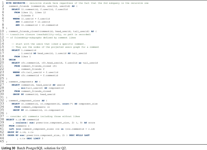
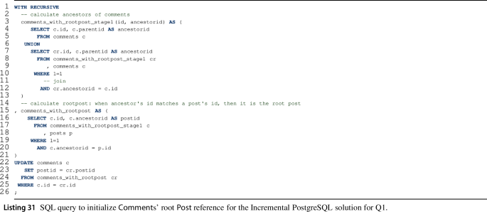
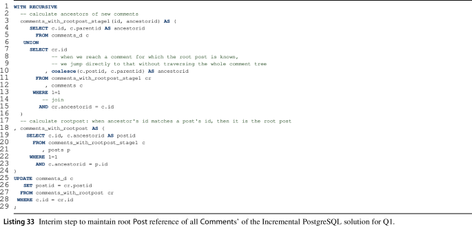
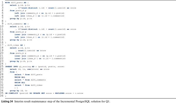
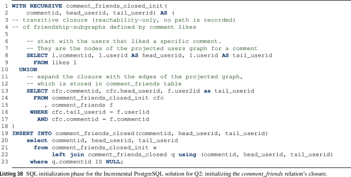
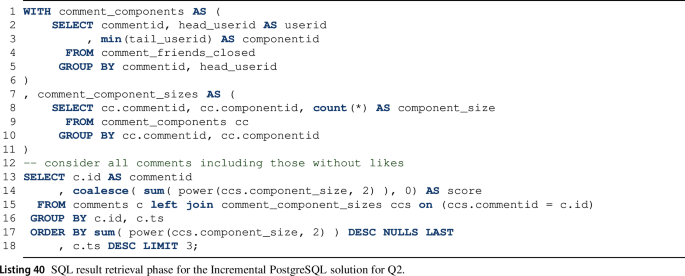
• Figure 14 contains the proof for the relational algebra formula for the join of relations with a positive delta (change set).

• Listings 41–42 contain the initial queries of the incremental Neo4j solution for Q2.

• Listings 43–44 contain the incremental maintenance queries of the Neo4j solution for Q2.

• Algorithm 5 shows a GraphBLAS algorithm to build the incidence matrix from an adjacency matrix.

Fig. 13

Relational algebra formula for join of relations with positive delta

Fig. 14

Proof for the relational algebra formula for join of relations with a positive delta (change set)

Fig. 15

Execution times of NMF solutions

Fig. 16

Execution times of Hawk solutions. Notation: IU: Incremental Update, IUQ: Incremental Update + Query

Fig. 17

Execution times of JastAdd solutions

Fig. 18

Execution times of YAMTL solutions

1.2 Comparison of solution variants

1.2.1 NMF

Figure 15 shows the results for the different variants of the NMF solution. The results show that the difference between the standard incremental mode and the transactional mode is marginal, i.e. the engine could not take advantage of propagating all changes at once instead of propagating each change separately. This is because the changes affect different parts of the dependency graph. However, executing these propagations in different threads also does not lead to speedups because there is usually one change propagation dominating the others. Instead, we see that the additional overhead of synchronization makes the parallel mode’s change propagation slightly slower in this case.

1.2.2 Hawk

Figure 16 shows the execution times of all different variants of the Hawk solution. Unfortunately, it appears that the initial load process did not complete within the timeout past model size 64 across the solutions: this is due to the use of monolithic single-file models in the benchmark framework, whereas Hawk is optimized towards models which have been fragmented into many files. The results show that the initial load is somewhat slower for the batch and incremental update (IU) solutions, as they need to calculate the derived attributes used to cache scores. These derived attributes allow the initial execution of the query to be much faster in the batch and IU modes than in the incremental update and query (IUQ) mode: the IUQ mode has to do a first full execution of the query. The updates are the slowest in the batch solution due to the need to both recalculate derived attributes and reserialize the changed social network model between updates. The IU mode has slightly faster updates, as it skips the reserialization and instead applies the changes directly to the graph used for querying. The IUQ mode speeds this up even further by replacing derived attributes with graph listeners, using them to detect changed comments and posts and re-score them.

1.2.3 JastAdd

Figure 17 shows the execution times of all different variants of the JastAdd solution. The results show that the approaches using bidirectional relations (Relast variants) are strictly better than their counterparts, both in terms of initial execution and time to propagate updates. As can be expected, the incremental variants are also slower than the batch variants in the initial query computation. However, because the JastAdd solution needs to sort the results also in the incremental case which dominates the complexity, the performance results for the incremental variants are not significantly faster than the batch variants. With unidirectional references as in the original metamodel, the change propagation in the incremental execution is even slower than the batch variant.

1.2.4 YAMTL

Figure 18 shows the execution times of all YAMTL solutions. They indicate that the performance improvements of the YAMTL-EI solutions over the purely implicit variant are rather small, except for Q2 where the time for an update propagation could be further reduced.

References

Abadi, D.: Data partitioning. In: Liu, L., Özsu, M.T. (eds.) Encyclopedia of Database Systems, 2nd edn. Springer, Berlin (2018). https://doi.org/10.1007/978-1-4614-8265-9_688
Acar, U.A.: Self-adjusting computation. Ph.D. thesis, Carnegie Mellon University, Pittsburgh, USA (2005)
Acar, U.A.: Self-adjusting computation (an overview). In: Proceedings of the 2009 ACM SIGPLAN Workshop on Partial Evaluation and Program Manipulation, pp. 1–6. ACM (2009)
Aho, A.V., Ullman, J.D.: The universality of data retrieval languages. In: POPL, pp. 110–120. ACM Press (1979). https://doi.org/10.1145/567752.567763
Angles, R., Antal, J.B., Averbuch, A., Boncz, P.A., Erling, O., Gubichev, A., Haprian, V., Kaufmann, M., Larriba-Pey, J., Martínez-Bazan, N., Marton, J., Paradies, M., Pham, M., Prat-Pérez, A., Spasic, M., Steer, B.A., Szárnyas, G., Waudby, J.: The LDBC social network benchmark. CoRR arXiv:2001.02299 (2020)
Anjorin, A., Buchmann, T., Westfechtel, B., Diskin, Z., Ko, H., Eramo, R., Hinkel, G., Samimi-Dehkordi, L., Zündorf, A.: Benchmarking bidirectional transformations: theory, implementation, application, and assessment. Softw. Syst. Model. 19(3), 647–691 (2020). https://doi.org/10.1007/s10270-019-00752-x
Bainomugisha, E., Carreton, A.L., Cutsem, Tv., Mostinckx, S., Meuter, Wd.: A survey on reactive programming. ACM Comput. Surv. 45(4), 521–5234 (2013). https://doi.org/10.1145/2501654.2501666
Barmpis, K., García-Domínguez, A., Bagnato, A., Abherve, A.: Monitoring model analytics over large repositories with Hawk and MEASURE. In: Model Management and Analytics for Large Scale Systems, pp. 87–123. Academic Press (2020). https://doi.org/10.1016/B978-0-12-816649-9.00014-4. http://www.sciencedirect.com/science/article/pii/B9780128166499000144
Beaudoux, O., Blouin, A., Barais, O., Jézéquel, J.: Active operations on collections. In: Model Driven Engineering Languages and Systems: 13th International Conference, MODELS 2010, Oslo, Norway, October 3-8, 2010, Proceedings, Part I. Lecture Notes in Computer Science, vol. 6394, pp. 91–105. Springer (2010)
Bergmann, G., Horváth, Á., Ráth, I., Varró, D.: A benchmark evaluation of incremental pattern matching in graph transformation. In: Ehrig, H., Heckel, R., Rozenberg, G., Taentzer, G. (eds.) Graph Transformations, 4th International Conference, ICGT 2008, Leicester, United Kingdom, September 7–13, 2008. Proceedings, Lecture Notes in Computer Science, vol. 5214, pp. 396–410. Springer (2008). https://doi.org/10.1007/978-3-540-87405-8_27
Bergmann, G., Horváth, Á., Ráth, I., Varró, D., Balogh, A., Balogh, Z., Ökrös, A.: Incremental evaluation of model queries over EMF models. In: Petriu, D.C., Rouquette, N., Haugen, Ø. (eds.) Model Driven Engineering Languages and Systems: 13th International Conference, MODELS 2010, Oslo, Norway, October 3–8, 2010, Proceedings, Part I, Lecture Notes in Computer Science, vol. 6394, pp. 76–90. Springer (2010). https://doi.org/10.1007/978-3-642-16145-2_6
Besnard, V., Jouault, F., Calvar, T.L., Tisi, M.: The TTC 2018 Social Media Case, by ATL and AOF. In: Garcia-Dominguez, A., Hinkel, G., Krikava, F. (eds.) Proceedings of the 11th Transformation Tool Contest, a part of the Software Technologies: Applications and Foundations (STAF 2018) federation of conferences, CEUR Workshop Proceedings. CEUR-WS.org (2018)
Bettini, L.: Implementing Domain-Specific Languages with Xtext and Xtend. Packt Publishing, Birmingham (2013)
Blakeley, J.A., Larson, P., Tompa, F.W.: Efficiently updating materialized views. In: SIGMOD, pp. 61–71. ACM Press (1986). https://doi.org/10.1145/16894.16861
Bögeholz, H., Brand, M., Todor, R.: In-database connected component analysis. In: ICDE, pp. 1525–1536. IEEE (2020). https://doi.org/10.1109/ICDE48307.2020.00135
Boronat, A.: Expressive and efficient model transformation with an internal DSL of Xtend. In: Proceedings of the 21th ACM/IEEE International Conference on MoDELS, pp. 78–88. ACM (2018)
Boronat, A.: YAMTL solution to the TTC 2018 social media case. In: Garcia-Dominguez, A., Hinkel, G., Krikava, F. (eds.) Proceedings of the 11th Transformation Tool Contest, a part of the Software Technologies: Applications and Foundations (STAF 2018) federation of conferences, CEUR Workshop Proceedings. CEUR-WS.org (2018)
Boronat, A.: Incremental execution of rule-based model transformation. Int. J. Softw. Tools Technol. Transf. (2020). https://doi.org/10.1007/s10009-020-00583-y
Brucker, A.D., Clark, T., Dania, C., Georg, G., Gogolla, M., Jouault, F., Teniente, E., Wolff, B.: Panel discussion: proposals for improving OCL. In: Proceedings of the 14th International Workshop on OCL and Textual Modelling, CEUR Workshop Proceedings, vol. 1285, pp. 83–99 (2014)
Buluç, A., Mattson, T., McMillan, S., Moreira, J.E., Yang, C.: Design of the GraphBLAS API for C. In: GABB at IPDPS, pp. 643–652. IEEE Computer Society (2017). https://doi.org/10.1109/IPDPSW.2017.117
Burckhardt, S., Leijen, D., Sadowski, C., Yi, J., Ball, T.: Two for the price of one: a model for parallel and incremental computation. SIGPLAN Not. 46(10), 427–444 (2011). https://doi.org/10.1145/2076021.2048101
Calvar, T.L., Chhel, F., Jouault, F., Saubion, F.: Using process algebra to statically analyze incremental propagation graphs. In: Hebig, R., Berger, T. (eds.) Proceedings of MODELS 2018 Workshops: ModComp, MRT, OCL, FlexMDE, EXE, COMMitMDE, MDETools, GEMOC, MORSE, MDE4IoT, MDEbug, MoDeVVa, ME, MULTI, HuFaMo, AMMoRe, PAINS co-located with ACM/IEEE 21st International Conference on Model Driven Engineering Languages and Systems (MODELS 2018), Copenhagen, Denmark, October, 14, 2018, CEUR Workshop Proceedings, vol. 2245, pp. 160–173. CEUR-WS.org (2018)
Calvar, T.L., Jouault, F., Chhel, F., Clavreul, M.: Efficient ATL incremental transformations. J. Object Technol. 18(3), 2:1-17 (2019). https://doi.org/10.5381/jot.2019.18.3.a2
Chirkova, R., Yang, J.: Materialized views. Found. Trends Databases 4(4), 295–405 (2012). https://doi.org/10.1561/1900000020
Davis, T.A.: Algorithm 1000: SuiteSparse:GraphBLAS: graph algorithms in the language of sparse linear algebra. ACM Trans. Math. Softw. 45(4), 44:1-44:25 (2019). https://doi.org/10.1145/3322125
Dong, G., Su, J.: Incremental maintenance of recursive views using relational calculus/SQL. SIGMOD Rec. 29(1), 44–51 (2000). https://doi.org/10.1145/344788.344808
Elekes, M., Antal, J.B., Szárnyas, G.: An analysis of the SIGMOD 2014 programming contest: complex queries on the LDBC social network graph. CoRR arXiv:2010.12243 (2020)
Elekes, M., Szárnyas, G.: An incremental GraphBLAS solution for the 2018 TTC Social Media case study. In: GrAPL at IPDPS, pp. 203–206. IEEE (2020). https://doi.org/10.1109/IPDPSW50202.2020.00045
Elekes, M., Szárnyas, G.: Incremental view maintenance in graph databases: a case study in Neo4j. In: Proceedings of the 27th PhD mini-symposium. Budapest University of Technology and Economics, Department of Measurement and Information Systems (2020). http://docs.inf.mit.bme.hu/paper-minisy20-elekes/elekes.pdf
Erling, O., Averbuch, A., Larriba-Pey, J., Chafi, H., Gubichev, A., Prat-Pérez, A., Pham, M., Boncz, P.A.: The LDBC social network benchmark: interactive workload. In: SIGMOD, pp. 619–630 (2015). https://doi.org/10.1145/2723372.2742786
Fan, W., Hu, C., Tian, C.: Incremental graph computations: doable and undoable. In: SIGMOD, pp. 155–169. ACM (2017). https://doi.org/10.1145/3035918.3035944
Forgy, C.L.: Rete: a fast algorithm for the many pattern/many object pattern match problem. Artif. Intell. 19(1), 17–37 (1982)
Francis, N., et al.: Cypher: an evolving query language for property graphs. In: SIGMOD, pp. 1433–1445. ACM (2018). https://doi.org/10.1145/3183713.3190657
Garcia-Dominguez, A.: Hawk solutions to the TTC 2018 Social Media Case. In: Garcia-Dominguez, A., Hinkel, G., Krikava, F. (eds.) Proceedings of the 11th Transformation Tool Contest, a part of the Software Technologies: Applications and Foundations (STAF 2018) Federation of Conferences, CEUR Workshop Proceedings. CEUR-WS.org (2018)
García-Domínguez, A., Hinkel, G., Krikava, F. (eds.): Proceedings of the 11th Transformation Tool Contest, Co-located with the 2018 Software Technologies: Applications and Foundations, TTC@STAF 2018, Toulouse, France, June 29, 2018, CEUR Workshop Proceedings, vol. 2310. CEUR-WS.org (2019). http://ceur-ws.org/Vol-2310
Giese, H., Wagner, R.: From model transformation to incremental bidirectional model synchronization. Softw. Syst. Model. 8(1), 21–43 (2009). https://doi.org/10.1007/s10270-008-0089-9
Green, A., et al.: Updating graph databases with Cypher. PVLDB (2019). https://doi.org/10.14778/3352063.3352139. http://www.vldb.org/pvldb/vol12/p2242-green.pdf
Griffin, T., Kumar, B.: Algebraic change propagation for semijoin and outerjoin queries. SIGMOD Rec. 27(3), 22–27 (1998). https://doi.org/10.1145/290593.290597
Gupta, A., Mumick, I.S., et al.: Maintenance of materialized views: problems, techniques, and applications. IEEE Data Eng. Bull. 18(2), 3–18 (1995)
Hammer, M.A., Dunfield, J., Headley, K., Labich, N., Foster, J.S., Hicks, M., Van Horn, D.: Incremental computation with names. In: Proceedings of the 2015 ACM SIGPLAN International Conference on Object-Oriented Programming, Systems, Languages, and Applications, pp. 748–766. ACM (2015)
Hammer, M.A., Phang, K.Y., Hicks, M., Foster, J.S.: Adapton: composable, demand-driven incremental computation. SIGPLAN Not. 49(6), 156–166 (2014). https://doi.org/10.1145/2666356.2594324
Hartmann, T., Fouquet, F., Jimenez, M., Rouvoy, R., Traon, Y.L.: Analyzing complex data in motion at scale with temporal graphs, pp. 596–601 (2017). https://doi.org/10.18293/SEKE2017-048. http://ksiresearchorg.ipage.com/seke/seke17paper/seke17paper_48.pdf
Hedin, G.: Reference attributed grammars. Informatica 24(3), 301 (2000)
Hedin, G., Magnusson, E.: JastAdd: an aspect-oriented compiler construction system. Sci. Comput. Program. 47, 37–58 (2003)
Hinkel, G.: NMF: A Modeling Framework for the .NET Platform. Technical report, Karlsruhe Institute of Technology, Karlsruhe (2016). http://nbn-resolving.org/urn:nbn:de:swb:90-537082
Hinkel, G.: Implicit incremental model analyses and transformations. Ph.D. thesis, Karlsruhe Institute of Technology (2017)
Hinkel, G.: An NMF solution to the Smart Grid case at the TTC 2017. In: García-Domínguez, A., Hinkel, G., Krikava, F. (eds.) Proceedings of the 10th Transformation Tool Contest (TTC 2017), Co-located with the 2017 Software Technologies: Applications and Foundations (STAF 2017), Marburg, Germany, July 21, 2017, CEUR Workshop Proceedings, vol. 2026, pp. 13–17. CEUR-WS.org (2017). http://ceur-ws.org/Vol-2026/paper5.pdf
Hinkel, G.: The TTC 2017 outage system case for incremental model views. In: Garcia-Dominguez, A., Hinkel, G., Krikava, F. (eds.) Proceedings of the 10th Transformation Tool Contest, a part of the Software Technologies: Applications and Foundations (STAF 2017) Federation of Conferences, CEUR Workshop Proceedings. CEUR-WS.org (2017)
Hinkel, G.: An NMF solution to the TTC 2018 Social Media Case. In: Garcia-Dominguez, A., Hinkel, G., Krikava, F. (eds.) Proceedings of the 11th Transformation Tool Contest, a part of the Software Technologies: Applications and Foundations (STAF 2018) Federation of Conferences, CEUR Workshop Proceedings. CEUR-WS.org (2018)
Hinkel, G.: NMF: a multi-platform modeling framework. In: Rensink, A., Cuadrado, J.S. (eds.) Theory and Practice of Model Transformations: 11th International Conference, ICMT 2018, Held as Part of STAF 2018, Toulouse, France, June 25–29, 2018. Proceedings. Springer (2018)
Hinkel, G.: The TTC 2018 social media case. In: Garcia-Dominguez, A., Hinkel, G., Krikava, F. (eds.) Proceedings of the 11th Transformation Tool Contest, a part of the Software Technologies: Applications and Foundations (STAF 2018) Federation of Conferences, CEUR Workshop Proceedings. CEUR-WS.org (2018)
Hinkel, G., Happe, L.: An NMF solution to the TTC train benchmark case. In: Rose, L., Horn, T., Krikava, F. (eds.) Proceedings of the 8th Transformation Tool Contest, a part of the Software Technologies: Applications and Foundations (STAF 2015) Federation of Conferences, CEUR Workshop Proceedings, vol. 1524, pp. 142–146. CEUR-WS.org (2015)
Jouault, F., Beaudoux, O.: On the use of active operations for incremental bidirectional evaluation of OCL. In: Proceedings of the 15th International Workshop on OCL and Textual Modeling, CEUR Workshop Proceedings, vol. 1512, pp. 35–45. Ottawa, Canada (2015)
Jouault, F., Beaudoux, O.: Efficient OCL-based incremental transformations. In: Proceedings of the 16th International Workshop in OCL and Textual Modeling, CEUR Workshop Proceedings, vol. 1756, pp. 121–136. Saint-Malo, France (2016)
Jouault, F., Kurtev, I.: Transforming models with ATL. In: Proceedings of the Model Transformations in Practice Workshop at MoDELS 2005, vol. Satellite, pp. 128–138. Springer (2005)
Jouault, F., Tisi, M.: Towards incremental execution of atl transformations. In: Tratt, L., Gogolla, M. (eds.) Theory and Practice of Model Transformations, pp. 123–137. Springer, Berlin (2010)
Kepner, J., Aaltonen, P., Bader, D.A., Buluç, A., Franchetti, F., Gilbert, J.R., Hutchison, D., Kumar, M., Lumsdaine, A., Meyerhenke, H., McMillan, S., Yang, C., Owens, J.D., Zalewski, M., Mattson, T.G., Moreira, J.E.: Mathematical foundations of the GraphBLAS. In: HPEC, pp. 1–9 (2016). https://doi.org/10.1109/HPEC.2016.7761646
Kepner, J., Gilbert, J.R. (eds.): Graph Algorithms in the Language of Linear Algebra, Software, Environments, Tools, vol. 22. SIAM (2011). https://doi.org/10.1137/1.9780898719918
Klabnik, S., Nichols, C.: The Rust Programming Language. No Starch Press, San Francisco (2018)
Knuth, D.E.: Semantics of context-free languages. Math. Syst. Theory 2(2), 127–145 (1968). https://doi.org/10.1007/BF01692511
Kolovos, D.S., Paige, R.F., Polack, F.: The epsilon object language (EOL). In: Model Driven Architecture: Foundations and Applications, Second European Conference, ECMDA-FA 2006, Bilbao, Spain, July 10–13, 2006, Proceedings, pp. 128–142 (2006). https://doi.org/10.1007/11787044_11
Magnusson, E., Hedin, G.: Circular reference attributed grammars: their evaluation and applications. Sci. Comput. Program. 68(1), 21–37 (2007)
Martínez, S., Tisi, M., Douence, R.: Reactive model transformation with atl. Sci. Compute. Program. 136, 1–16 (2017). https://doi.org/10.1016/j.scico.2016.08.006
Mattson, T., Davis, T.A., Kumar, M., Buluç, A., McMillan, S., Moreira, J.E., Yang, C.: LAGraph: a community effort to collect graph algorithms built on top of the GraphBLAS. In: GrAPL at IPDPS, pp. 276–284 (2019). https://doi.org/10.1109/IPDPSW.2019.00053
McSherry, F., Murray, D.G., Isaacs, R., Isard, M.: Differential dataflow. In: CIDR (2013). http://cidrdb.org/cidr2013/Papers/CIDR13_Paper111.pdf
Mey, J., Kühn, T., Schöne, R., Aßmann, U.: Reusing static analysis across different domain-specific languages using reference attribute grammars. Art Sci. Eng. Program. (2020). https://doi.org/10.22152/programming-journal.org/2020/4/15
Mey, J., Schöne, R., Hedin, G., Söderberg, E., Kühn, T., Fors, N., Öqvist, J., Aßman, U.: Continuous model validation using reference attribute grammars. In: Proceedings of the 11th International Conference on Software Language Engineering (2018)
Monge, A.E., Elkan, C.: An efficient domain-independent algorithm for detecting approximately duplicate database records. In: DMKD (1997)
Murray, D.G., McSherry, F., Isaacs, R., Isard, M., Barham, P., Abadi, M.: Naiad: a timely dataflow system. In: SIGOPS, pp. 439–455. ACM (2013). https://doi.org/10.1145/2517349.2522738
Murray, D.G., McSherry, F., Isard, M., Isaacs, R., Barham, P., Abadi, M.: Incremental, iterative data processing with timely dataflow. Commun. ACM 59(10), 75–83 (2016). https://doi.org/10.1145/2983551
Needham, M., Hodler, A.E.: Graph Algorithms: Practical Examples in Apache Spark and Neo4j. O’Reilly Media, Sebastopol (2019)
Peldszus, S., Bürger, J., Strüber, D.: Detecting and preventing power outages in a smart grid using emoflon. In: García-Domínguez, A., Hinkel, G., Krikava, F. (eds.) Proceedings of the 10th Transformation Tool Contest (TTC 2017), Co-located with the 2017 Software Technologies: Applications and Foundations (STAF 2017), Marburg, Germany, July 21, 2017, CEUR Workshop Proceedings, vol. 2026, pp. 19–23. CEUR-WS.org (2017). http://ceur-ws.org/Vol-2026/paper17.pdf
Pugh, W., Teitelbaum, T.: Incremental computation via function caching. In: Proceedings of the 16th ACM SIGPLAN-SIGACT symposium on Principles of programming languages, pp. 315–328. ACM (1989)
Raasveldt, M., Mühleisen, H.: DuckDB: an embeddable analytical database. In: SIGMOD, pp. 1981–1984. ACM (2019). https://doi.org/10.1145/3299869.3320212
Ramalingam, G., Reps, T.: A categorized bibliography on incremental computation. In: Proceedings of the 20th ACM SIGPLAN-SIGACT symposium on Principles of programming languages, pp. 502–510. ACM (1993)
Reiss, S.P.: An approach to incremental compilation. In: Proceedings of the 1984 SIGPLAN Symposium on Compiler Construction, SIGPLAN ’84, pp. 144–156. ACM, New York, NY, USA (1984). https://doi.org/10.1145/502874.502889
Reps, T.: Optimal-time incremental semantic analysis for syntax-directed editors. In: Proceedings of the 9th ACM SIGPLAN-SIGACT Symposium on Principles of Programming Languages, POPL ’82, pp. 169–176. ACM, New York, NY, USA (1982). https://doi.org/10.1145/582153.582172
Schöne, R., Mey, J.: A JastAdd-based solution to the TTC 2018 social media case. In: Garcia-Dominguez, A., Hinkel, G., Krikava, F. (eds.) Proceedings of the 11th Transformation Tool Contest, a part of the Software Technologies: Applications and Foundations (STAF 2018) federation of conferences, CEUR Workshop Proceedings. CEUR-WS.org (2018)
Sebaa, A., Tari, A.: Materialized view maintenance: issues, classification, and open challenges. Int. J. Coop. Inf. Syst. 28(1), 19300011–193000159 (2019). https://doi.org/10.1142/S0218843019300018
Sedgewick, R., Wayne, K.: Algorithms, 4th edn. Addison-Wesley, Boston (2011)
Szárnyas, G.: Query, analysis, and benchmarking techniques for evolving property graphs of software systems. Ph.D. dissertation, Budapest University of Technology and Economics (2019). http://hdl.handle.net/10890/13133
Szárnyas, G., Izsó, B., Ráth, I., Varró, D.: The train benchmark: cross-technology performance evaluation of continuous model queries. Softw. Syst. Model. (2017). https://doi.org/10.1007/s10270-016-0571-8
Szárnyas, G., Semeráth, O., Ráth, I., Varró, D.: The TTC 2015 train benchmark case for incremental model validation. In: TTC at STAF, pp. 129–141 (2015). http://ceur-ws.org/Vol-1524/paper2.pdf
Tarjan, R.: Depth-first search and linear graph algorithms. SIAM J. Comput. 1(2), 146–160 (1972)
Varró, D., Bergmann, G., Hegedüs, Á., Horváth, Á., Ráth, I., Ujhelyi, Z.: Road to a reactive and incremental model transformation platform: three generations of the VIATRA framework. Softw. Syst. Model. 15(3), 609–629 (2016). https://doi.org/10.1007/s10270-016-0530-4
Vogt, H.H., Swierstra, S.D., Kuiper, M.F.: Higher order attribute grammars. In: PLDI ’89. ACM, New York, NY, USA (1989). https://doi.org/10.1145/73141.74830
Waudby, J., Steer, B.A., Prat-Pérez, A., Szárnyas, G.: Supporting dynamic graphs and temporal entity deletions in the LDBC Social Network Benchmark’s data generator. In: GRADES-NDA at SIGMOD, pp. 8:1–8:8. ACM (2020). https://doi.org/10.1145/3398682.3399165
Zhang, Y., Azad, A., Hu, Z.: FastSV: a distributed-memory connected component algorithm with fast convergence. In: PPSC, pp. 46–57. SIAM (2020). https://doi.org/10.1137/1.9781611976137.5
Zhao, K., Yu, J.X.: All-in-one: graph processing in RDBMSs revisited. In: SIGMOD, pp. 1165–1180. ACM (2017). https://doi.org/10.1145/3035918.3035943
Acknowledgements
We would like to thank Frank McSherry for providing an initial implementation of the Differential Dataflow solution. René Schöne was supported by German Federal Ministry of Education and Research within the research project “OpenLicht”. Márton Elekes’s research was funded by the European Commission and the Hungarian Authorities (NKFIH) through the Arrowhead Tools project (EU Grant Agreement No. 826452, NKFIH Grant 2019-2.1.3-NEMZ ECSEL-2019-00003) and by the NRDI Fund based on the charter of bolster issued by the NRDI Office under the auspices of the Ministry for Innovation and Technology. Gábor Szárnyas was partially supported by the SQIREL-GRAPHS NWO project.
Funding
Open access funding provided by Budapest University of Technology and Economics.
Author information
Authors and Affiliations
Corresponding author
Additional information
Communicated by Alexander Egyed.
Publisher's Note
Springer Nature remains neutral with regard to jurisdictional claims in published maps and institutional affiliations.