Amplified tropical Pacific rainfall variability related to background SST warming

Abstract

Previous studies have found that under global warming, El Niño/Southern Oscillation (ENSO)-related rainfall variability will become enhanced over the tropical central-eastern Pacific and weakened over the western Pacific. The climatological sea surface temperature (SST) warming pattern exhibits a warming center in the equatorial eastern Pacific in projections. How this pattern contributes to projected changes in ENSO-driven rainfall variability has not been fully addressed. Here, we use “time-slice” experiments to investigate the response of interannual variability in tropical Pacific rainfall in boreal winter to a warming background SST and associated physical mechanisms. A high-resolution Atmosphere General Circulation Model is driven by the detrended observational SST (1979–2003) plus a warming pattern from the coupled model under the A1B emission scenario (2075–2099). The results show that precipitation interannual variability over the tropical central-eastern Pacific will be enhanced more than the surrounding regions under warming, which is mostly contributed by a faster increase in rainfall amount during the El Niño year relative to non-El Niño years. Based on a moisture budget analysis, both the dynamic and thermodynamic components in the vertical advection of climatological specific humidity contribute to the enhancement of El Niño-induced precipitation anomalies in the tropical central-eastern Pacific where the dynamic effect is dominant. Moist static energy budget analysis further illustrates that vertical velocity is enhanced due to the increased transport of moist static energy from the lower troposphere into the middle-upper troposphere and the intensified warming effect of cloud longwave radiation caused by the increase of high cloud amount and altitude.

1 Introduction

Under a warming climate, projected changes in the interannual variability in precipitation have substantial impacts on global ecosystems, agriculture and the economy. Changes in precipitation variability are particularly impact-relevant since these changes strongly affect the extremes that are more difficult for society to adapt to. Changes in precipitation interannual variability under global warming have been a hot topic in recent years (Power et al. 2013; Chung et al. 2014; Watanabe et al. 2014; Huang and Xie 2015; Huang 2016; Pendergrass et al. 2017; He and Li 2019). In the Sixth Assessment Report of the Intergovernmental Panel on Climate Change (IPCC), a new chapter will focus on this topic. Under global warming, global precipitation interannual variability is projected to increase with maxima in the tropical Pacific Ocean and monsoon region (Rind et al. 1989; Tsonis 1996; Räisänen 2002; Giorgi and Bi 2005; Pendergrass et al. 2017; He and Li 2019). An increase in global precipitation interannual variability is contributed by an increase in moisture and a decrease in circulation (Pendergrass et al. 2017; He and Li 2019). Essentially, changes in circulation are region-dependent, and these changes are projected to be weakened almost everywhere except over the equatorial Pacific (He and Li 2019).

For the maxima of increasing precipitation interannual variability over the tropical Pacific, most work has recently focused on ENSO-driven rainfall variability (Power et al. 2013; Chung et al. 2014; Huang and Xie 2015; Huang 2016). ENSO-driven rainfall variability is projected to be reinforced over the tropical central-eastern Pacific and weakened over the western Pacific (Müller and Roeckner 2008; Watanabe et al. 2012; Power et al. 2013; Cai et al. 2015; Huang and Xie 2015; Huang 2016). The intensification of the ENSO-induced tropical central-eastern Pacific is contributed by climatological SST warming patterns, amplitude changes in ENSO-related SST variability, structural changes in ENSO-related SST variability, and increases in mean-state moisture content (Huang and Xie 2015; Huang 2016). Among these patterns, the climatological surface warming pattern is the dominant dynamic contributor to enhanced precipitation anomalies in the tropical central-eastern Pacific (Power et al. 2013), in which SST warming pattern play a more important role relative to uniform warming (Zheng et al. 2016). However, previous studies have not demonstrated the physical mechanism by which climatological SST warming influences the enhanced ENSO-driven rainfall variability. The response of climatological SST over the tropical Pacific to greenhouse gas forcing in most coupled models is characterized by faster warming on the central-eastern Pacific compared to surrounding regions (Xie et al. 2010; Tokinaga et al. 2012), although La Niña-like warming pattern is also seen in few models (Kohyama et al. 2017; Seager et al. 2019). It is necessary to investigate the physical mechanism of enhanced ENSO-driven rainfall variability in response to a robust background SST warming.

To isolate the effect of climatological SST warming, we use the Atmosphere General Circulation Model (AGCM) driven by SST boundary conditions with unchanged interannual variability to investigate how background SST warming contributes to the tropical Pacific rainfall interannual variability. The following questions will be addressed in this study: (1) How will precipitation interannual variability over the tropical Pacific change under global warming based on the premise of unchanged ENSO variability? (2) Is the precipitation interannual variability over the tropical Pacific region dominated by El Niño-induced precipitation variability? (3) Which physical processes play a major role in the changes in precipitation interannual variability over the tropical central-eastern Pacific?

The remainder of this paper is arranged as follows. In Sect. 2, the data and analysis methods used in this study are described. In Sect. 3, the model performance is evaluated for the tropical Pacific. Changes in precipitation interannual variability and associated physical mechanisms are shown in Sects. 4, 5. A summary and discussion are presented in Sect. 6.

2 Data and methods

• a.
  

  Observational and reanalysis data

  Monthly precipitation from the Global Precipitation Climatology Project (GPCP; Adler et al. 2003) and monthly meridional and zonal winds at 850 hPa from the European Centre for Medium-Range Weather Forecasts (ECMWF) interim reanalysis (ERA-Interim; Dee et al. 2011) are used in this paper to evaluate model performance over the tropical Pacific. All datasets cover the 1979–2003 period.

• b. Model and experiments

• a)
  

  MRI-AGCM3.1H

  MRI-AGCM3.1H is a high-resolution version of MRI-AGCM3.1, developed by the Japan Meteorological Agency (JMA) and Meteorological Research Institute (MRI; Mizuta et al. 2006). The horizontal resolution is 60 km, which is 0.56° $\times$ 0.56°. There are 60 model levels in the vertical direction (up to 0.1 hPa). The dynamic core, which is a full primitive equation system (Kanamitsu et al. 1983), is implemented. A spectral transform method of spherical harmonics is used in the model. The vertical coordinate is a sigma-pressure hybrid coordinate. The cumulus convection scheme in MRI-AGCM3.1H is proposed by Arakawa and Schubert (1974). The horizontal and vertical advection schemes are conservative semi-Lagrangian schemes and standard semi-Lagrangian schemes (with conserved mass, water vapor and cloud water), respectively.

  The experimental design includes a present-day climate simulation and future climate simulation. Figure 1 shows the decomposition of forced boundary SST in both experiments. These two experiments are forced by the same SST interannual variability spatial pattern (Fig. 1a, b). The present-day climate simulation is a typical Atmospheric Model Intercomparison Project (AMIP) run from 1979 to 2003 (HP) driven by the observed SST and sea ice data of HadISST1 (Rayner et al. 2003). This simulation is used as a control run. The future climate simulation is a “time-slice” run from 2075 to 2099 (HF). The boundary SST of future experiments comprises observational detrended observed SST anomalies (1979–2003; Fig. 1b) and a warming pattern obtained from the Coupled Model Intercomparison Project phase 3 (CMIP3) multi- model mean under the A1B emission scenario (2075–2099; Fig. 1c). It is noted that the future SST also has a linear trend during 2075–2099 from the CMIP3 multi-model mean (Mizuta 2008). More details are described in Mizuta (2008). The design is suitable to investigate the response of the interannual variability in tropical Pacific rainfall to climatological SST warming without changes in SST variability.

  Fig. 1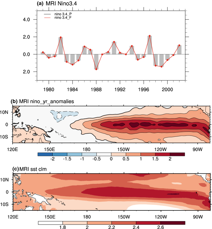

  

  a DJF mean Nino 3.4 index. b Spatial distribution of boreal winter SST anomalies during El Niño years in the present-day experiment (shaded, unit: K) and future experiment (contour, unit: K) of MRI-AGCM3.1H. c Climatological DJF mean SST warming patterns projected by CMIP3 MME which is used as a SST boundary condition to drive MRI-AGCM3.1H. The gray bar and red line in (a) indicate the results of the present and future runs (a linear trend during the period is removed), respectively

• b) AMIP models in CMIP5

  Monthly mean precipitation, zonal wind at 850 hPa (U850) and meridional wind at 850 hPa (V850) from 24 Atmospheric Model Intercomparison Project (AMIP) outputs of CMIP5 (Taylor et al. 2012) are also used to examine model performance. More details about the 24 AMIP models are shown in Table 1. A common period of 1979–2003 is chosen in the study.

  Table 1 Description of the CMIP5 stand-alone atmospheric general circulation models used in the paper

  In this study, a 25-year linear trend is removed prior to conducting the interannual variability analyses in both observations and models. The Niño-3.4 index is defined as the area-averaged SSTA over the region 5° N–5° S, 120°–170° W. The selection of El Niño events is based on the threshold of one-half standard deviation of December–January–February (DJF) mean Niño-3.4 index.

• c. Analytical methods

• 1.
  

  Moisture budget analysis

  A moisture budget analysis (Trenberth and Guillemot 1995; Seager et al. 2010; Chou and Lan 2012; Chou et al. 2013) is used on the interannual time scale to understand the mechanisms responsible for precipitation anomalies. The vertically integrated moisture equation is written as follows:

  $$P^{\prime} \approx E^{\prime} - \left\langle {\bar{\overset{\lower0.5em\hbox{$\smash{\scriptscriptstyle\rightharpoonup}$}} {u} } \cdot \nabla_{h} q^{\prime}} \right\rangle - \left\langle {\overset{\lower0.5em\hbox{$\smash{\scriptscriptstyle\rightharpoonup}$}} {u}^{\prime} \cdot \nabla_{h} \bar{q}} \right\rangle - \left\langle {\bar{\omega } \cdot \partial_{p} q^{\prime}} \right\rangle - \left\langle {\omega^{\prime} \cdot \partial_{p} \bar{q}} \right\rangle + NL.$$

  (1)

  where primes denote the monthly anomaly; overbars denote the monthly mean; angle brackets denote vertical integration from the surface to the top of the atmosphere (TOA); subscript h represents the horizontal direction; subscript p represents pressure; q denotes specific humidity; $\overset{\lower0.5em\hbox{$\smash{\scriptscriptstyle\rightharpoonup}$}} {u}$ denotes horizontal wind; $\omega$ denotes vertical pressure velocity; P and E represent precipitation and evaporation, respectively; and NL represents all nonlinear terms.

  According to Eq. (1), the changes in precipitation anomalies between future and present-day can be determined as follows:

  $$ \begin{aligned}\Delta P^{\prime} &\approx \Delta E^{\prime} - \Delta \left\langle {\bar{\overset{\lower0.5em\hbox{$\smash{\scriptscriptstyle\rightharpoonup}$}} {u} } \cdot \nabla_{h} q^{\prime}} \right\rangle \\&\quad- \Delta \left\langle {\overset{\lower0.5em\hbox{$\smash{\scriptscriptstyle\rightharpoonup}$}} {u}^{\prime} \cdot \nabla_{h} \bar{q}} \right\rangle - \Delta \left\langle {\bar{\omega } \cdot \partial_{p} q^{\prime}} \right\rangle \\&\quad- \Delta \left\langle {\omega^{\prime} \cdot \partial_{p} \bar{q}} \right\rangle + NL,\end{aligned} $$

  (2)

  where the $\Delta$ denote changes between the future and present day. Each term on the right side of the equation, except for the evaporation term, can be further divided into two parts, which are caused by changes in the dynamic ($\Delta \bar{\overset{\lower0.5em\hbox{$\smash{\scriptscriptstyle\rightharpoonup}$}} {u} }$, $\Delta \overset{\lower0.5em\hbox{$\smash{\scriptscriptstyle\rightharpoonup}$}} {u}^{\prime}$, $\Delta \bar{\omega }$, $\Delta \omega^{\prime}$) and thermodynamic ($\Delta \bar{q}$, $\Delta q^{\prime}$) components, respectively. Therefore, Eq. (2) can be further transformed to the following expression:

  $$ \begin{aligned}\Delta P^{\prime} &\approx \Delta E^{\prime} - \left\langle {\Delta \bar{\overset{\lower0.5em\hbox{$\smash{\scriptscriptstyle\rightharpoonup}$}} {u} } \cdot \nabla_{h} q^{\prime}} \right\rangle - \left\langle {\bar{\overset{\lower0.5em\hbox{$\smash{\scriptscriptstyle\rightharpoonup}$}} {u} } \cdot \nabla_{h} (\Delta q^{\prime})} \right\rangle \\&\quad - \left\langle {\Delta \overset{\lower0.5em\hbox{$\smash{\scriptscriptstyle\rightharpoonup}$}} {u}^{\prime} \cdot \nabla_{h} \bar{q}} \right\rangle - \left\langle {\overset{\lower0.5em\hbox{$\smash{\scriptscriptstyle\rightharpoonup}$}} {u}^{\prime} \cdot \nabla_{h} \left( {\Delta \bar{q}} \right)} \right\rangle - \left\langle {\Delta \bar{\omega } \cdot \partial_{p} q^{\prime}} \right\rangle \\&\quad - \left\langle {\Delta \bar{\omega } \cdot \partial_{p} \left( {\Delta q^{\prime}} \right)} \right\rangle - \left\langle {\Delta \omega^{\prime} \cdot \partial_{p} \bar{q}} \right\rangle \\&\quad - \left\langle {\omega^{\prime} \cdot \partial_{p} \left( {\Delta \bar{q}} \right)} \right\rangle + NL,\end{aligned} $$

  (3)

• 2. Moist static energy budget

  In the tropics and subtropical monsoon regions, vertical motion is largely constrained by the moist static energy (MSE) budget (Neelin and Held 1987; Neelin 2007), which can be expressed as follows:

  $$ \begin{aligned}&\partial_{t} \left\langle {\left( {c_{p} T + L_{v} q} \right)} \right\rangle^{\prime } + \left\langle {\overset{\lower0.5em\hbox{$\smash{\scriptscriptstyle\rightharpoonup}$}} {u} \cdot \nabla_{h} \left( {c_{p} T + L_{v} q} \right)} \right\rangle^{\prime }\\&\quad + \left\langle {w \cdot \partial_{p} h} \right\rangle^{\prime } = F_{\text{net}}^{\prime }\end{aligned} $$

  (4)

  where MSE is represented by $h = c_{p} T + L_{v} q + \varphi$; $c_{p}$ and $L_{v}$ denote specific heat at constant pressure and latent heat of vaporization, respectively; T represents air temperature; ${\text{s}} = c_{p} T + L_{v} q$ represents moist enthalpy; $\varphi$ denotes geopotential; and $F_{\text{net}}$ is the net MSE flux coming into an atmospheric column (Wu et al. 2017):

  $$ \begin{aligned}F_{\text{net}}& = \left( {S_{t}^{ \downarrow } - S_{t}^{ \uparrow } - R_{t}^{ \uparrow } } \right) \\&\quad- \left( { - S_{s}^{ \uparrow } + S_{s}^{ \downarrow } - R_{s}^{ \uparrow } + R_{s}^{ \downarrow } - LH - SH} \right).\end{aligned} $$

  (5)

  where the right 9 terms of Eq. (5) are downward shortwave radiative flux at the TOA, upward shortwave radiative flux at the TOA, upward longwave radiative flux at the TOA, and upward shortwave radiative flux at the surface, downward shortwave radiative flux at the surface, upward longwave radiative flux at the surface, downward longwave radiative flux at the surface, latent heat (LH) flux and sensible heat (SH) flux. The four solar radiation terms and three longwave radiation terms were merged together and are known as the changes in net solar radiation flux ($\Delta S^{\prime}$) and net longwave radiation flux ($\Delta R^{\prime}$), respectively. The net longwave radiative flux anomalies are separated into cloud-related ($\Delta R^{\prime}_{\text{cloud}}$) and clear-sky components ($\Delta R^{\prime}_{\text{clearsky}}$). Finally, Eq. (5) is simplified as follows:

  $$\Delta F_{\text{net}}^{\prime } = \Delta R^{\prime}_{\text{cloud}} + \Delta R^{\prime}_{\text{clearsky}} + \Delta S^{\prime} + \Delta LH^{\prime} + \Delta SH^{\prime}.$$

  (6)

  Since the time tendency term [first term in Eq. (4)] is much smaller than the other terms on the interannual time scale, this term is negligible. The MSE equation can be transformed as follows:

  $$ \begin{aligned}\left\langle {\omega^{\prime} \cdot \partial_{p} \bar{h}} \right\rangle &\approx F_{\text{net}}^{\prime } - \left\langle {\bar{\overset{\lower0.5em\hbox{$\smash{\scriptscriptstyle\rightharpoonup}$}} {u} } \cdot \nabla_{h} \left( {c_{p} T + L_{v} q} \right)^{\prime } } \right\rangle \\&\quad- \left\langle {\overset{\lower0.5em\hbox{$\smash{\scriptscriptstyle\rightharpoonup}$}} {u}^{\prime} \cdot \nabla_{h} \overline{{\left( {c_{p} T + L_{v} q} \right)}} } \right\rangle \\&\quad- \left\langle {\bar{\omega } \cdot \partial_{p} h^{\prime}} \right\rangle + NL,\end{aligned} $$

  (7)

  Similar to the moisture equation, each term on the right side of the equation except the evaporation term can be further divided into two dynamic ($\Delta \bar{\overset{\lower0.5em\hbox{$\smash{\scriptscriptstyle\rightharpoonup}$}} {u} }$, $\Delta \overset{\lower0.5em\hbox{$\smash{\scriptscriptstyle\rightharpoonup}$}} {u}^{\prime}$, $\Delta \bar{\omega }$, $\Delta \omega^{\prime}$) and thermodynamic components ($\Delta \bar{h}$, $\Delta h^{\prime}$, $\Delta \overline{{\left( {c_{p} T + L_{v} q} \right)}}$, $\Delta \left( {c_{p} T + L_{v} q} \right)^{\prime }$), respectively. Equation (7) can be transformed as follows:

  $$ \begin{aligned}\left\langle {\Delta \omega^{\prime} \cdot \partial_{p} \bar{h}} \right\rangle &\approx \Delta F_{\text{net}}^{\prime } - \left\langle {\omega^{\prime} \cdot \partial_{p} \left( {\Delta \bar{h}} \right)} \right\rangle \\&\quad - \left\langle {\Delta \bar{\overset{\lower0.5em\hbox{$\smash{\scriptscriptstyle\rightharpoonup}$}} {u} } \cdot \nabla_{h} \left( {c_{p} T + L_{v} q} \right)^{\prime } } \right\rangle \\&\quad - \left\langle {\bar{\overset{\lower0.5em\hbox{$\smash{\scriptscriptstyle\rightharpoonup}$}} {u} } \cdot \nabla_{h} \left( {\Delta \left( {c_{p} T + L_{v} q} \right)^{\prime } } \right)} \right\rangle \\&\quad - \left\langle {\Delta \overset{\lower0.5em\hbox{$\smash{\scriptscriptstyle\rightharpoonup}$}} {u}^{\prime} \cdot \nabla_{h} \overline{{\left( {c_{p} T + L_{v} q} \right)}} } \right\rangle \\&\quad- \left\langle {\overset{\lower0.5em\hbox{$\smash{\scriptscriptstyle\rightharpoonup}$}} {u}^{\prime} \cdot \nabla_{h} \left( {\Delta \overline{{\left( {c_{p} T + L_{v} q} \right)}} } \right)} \right\rangle \\&\quad - \left\langle {\Delta \bar{\omega } \cdot \partial_{p} h^{\prime}} \right\rangle - \left\langle {\bar{\omega } \cdot \partial_{p} \Delta h^{\prime}} \right\rangle + NL,\end{aligned} $$

  (8)

3 Basic evaluation of MRI-AGCM3.1H in the tropical Pacific

3.1 Mean state

The mean state of precipitation and circulations in the tropical Pacific in boreal winter are evaluated. Compared with the GPCP and ERA-Interim data, MRI-AGCM3.1H reasonably reproduces the climatological precipitation and low-level wind field (Fig. 2a, b). In detail, two significant precipitation centers, the Intertropical Convergence Zone (ITCZ) and the South Pacific Convergence Zone (SPCZ), are well captured but with larger magnitudes, especially for the tropical Northeast Pacific region (Fig. 2c) which is an chronic bias also seen in the previous model version (Kitoh and Arakawa 1999). The low-level trades are also reasonably reproduced by MRI-AGCM3.1H. The near-equatorial low-level wind is stronger, especially for the Northeast Pacific region.

Fig. 2

a Distribution of boreal winter climatological precipitation (shaded, unit: mm/day) and 850-hPa winds (vectors, unit: m/s) in the observation. b Same as in (a) but for the present-day simulation of MRI-AGCM3.1H. c Same as in (a) but for the differences between the observation and present-day simulation of MRI-AGCM3.1H

To quantitatively evaluate the model performance, a Taylor diagram is drawn in Fig. 3a–c. The radial distance indicates the model spatial variability in precipitation and low-level winds with respect to the observation. The azimuthal location indicates the pattern correlation between the model simulation and observation. The root mean square difference is related to the above two quantities. The ratio of standard deviation and pattern correlation of mean state precipitation are 1.31 and 0.84, respectively (Fig. 3a). The model simulations of low-level winds (U850, V850) agree with the observations better than precipitation (Fig. 3b, c). The ratio of standard deviation and pattern correlation of climatological U850 (V850) are 1.10 (1.02) and 0.92 (0.84), respectively. The performance of MRI-AGCM3.1H in climatological precipitation and low-level wind is better than half of the AMIP models in CMIP5. Therefore, MRI-AGCM3.1H has a good performance in simulating climatological rainfall and low-level winds. In addition, previous studies also illustrate that MRI_AGCM3.1H reasonably reproduce the East Asia monsoon precipitation and tropical cyclones (Sugi et al. 2009; Murakami and Sugi 2010; Kusunoki et al. 2011; Mizuta et al. 2011). The intensity and position of summer precipitation over East Asia is well captured by MRI_AGCM3.1H (Kusunoki et al. 2011). The mean-state and interannual variations of tropical cyclone genesis number are reasonably reproduced by MRI_AGCM3.1H, especially for Western North Pacific, North Atlantic and Southern Indian Ocean (Sugi et al. 2009; Murakami and Sugi 2010). Besides, the spatial distribution of extratropical cyclones during boreal winter is also well simulated (Mizuta et al. 2011).

Fig. 3

Taylor diagram of boreal winter mean precipitation (unit: mm/day) (a), mean U850 (unit: m/s) (b), mean V850 (unit: m/s) (c), and precipitation standard deviation (unit: mm/day) (d). Label 1 indicates MRI-AGCM 3.1H and label 2-25 indicates 24 AMIP outputs of CMIP5

3.2 Interannual variability

The model capability in reproducing precipitation interannual variability is also evaluated (Fig. 4a–c). Here, the standard deviation of precipitation is used to represent the intensity of the interannual variability. The interannual variability in precipitation is larger over the central Pacific than in other tropical Pacific regions (Fig. 4a). MRI-AGCM3.1H reasonably reproduced the maximal center of precipitation interannual variability, although with a larger magnitude than the observation (Figs. 4b, c). Moreover, the maximum center of the precipitation interannual variability was located more north and east than the observation. Based on the Taylor diagram, the ratios of standard deviation and pattern correlation of precipitation interannual variability in MRI-AGCM3.1H are 1.02 and 0.68, respectively (Fig. 3d). The performance in the spatial distribution of precipitation variability in MRI-AGCM3.1H is better than over 60% of CMIP5 models. In brief, MRI-AGCM3.1H captured the observed features of mean-state and interannual variability in precipitation.

Fig. 4

a Distribution of the standard deviation of tropical central-east Pacific winter rainfall (unit: mm/day) in the observation. b Same as in (a) but for the present-day simulation of MRI-AGCM3.1H. c Same as in (a) but for the differences between the observation and present-day simulation of MRI-AGCM3.1H. d Same as in (a) but for the changes between the future and present-day simulations of MRI-AGCM3.1H. The black dashed lines in (d) indicate the region with maximal changes in the precipitation standard deviation

4 Changes in precipitation interannual variability related to climatological SST warming

Figure 4d shows the projected changes in the standard deviation of precipitation between the future and present day. MRI-AGCM3.1H projects that precipitation interannual variability over the tropical central-eastern Pacific (5° S–3° N, 100° W–150° W) would increase more than the surrounding regions in a future warmer climate.

To investigate the mechanisms for precipitation interannual variability intensification, the regional mean rainfall index is calculated over the central-eastern Pacific (5° S–3° N, 100° W–150° W) region (Fig. 5a). The correlation coefficient between the present rainfall index and its changes under global warming is 0.67 (statistically significant at the 1% level). This positive correlation indicates an intensification of precipitation interannual variability. Specifically, in the present day climate, rainfall in El Niño years is more than that in neutral and La Niña years over the central-eastern Pacific. Coincidently, rainfall in El Niño years over the central-eastern Pacific is projected to increase more than that in neutral and La Niña years under global warming. Therefore, the precipitation differences between El Niño years and non-El Niño years will increase under a warming climate and precipitation interannual variability will increase. Next, the spatial pattern of El Niño-induced precipitation anomalies in the tropical Pacific is examined in Fig. 5b. El Niño-induced positive precipitation anomalies in the tropical central-eastern Pacific will be strengthened under global warming (statistically significant at the 1% level), although El Niño SST anomalies are unchanged between the future and present-day simulations. Furthermore, we note that the increase in El Niño-induced positive precipitation anomalies over the tropical central-eastern Pacific is consistent with the enhancement of precipitation interannual variability. In short, the intensification of precipitation interannual variability over the tropical central-eastern Pacific is due to the faster increase in positive interannual rainfall during El Niño years compared with non-El Niño years. In the next section, we investigate the underlying physical mechanisms.

Fig. 5

a DJF mean rainfall index (unit: mm/day) averaged over the tropical central-east Pacific (5° S–3° N, 100° W–150° W) from MRI-AGCM3.1H. b Changes in Nino 3.4 related precipitation (unit: mm/day) between the future (2075–2099) and present day (1979–2003) in MRI-AGCM3.1H. The gray bar in (a) indicates changes in the DJF mean rainfall index between the future and present day. The blue (light blue) line in (a) indicates the tropical central-east Pacific rainfall index in the future simulation (present-day simulation). The yellow shadow in (a) indicates El Niño years. The black dashed lines in (b) are the same as in Fig. 3c. The gray slashed line indicates the areas with statistical confidence at the 99% level

5 Mechanisms for increased El Niño-induced rainfall anomalies in response to background SST warming

To investigate mechanisms leading to the distinct changes in rainfall anomalies during El Niño years and non-El Niño years over the tropical central-eastern Pacific, a moisture budget analysis is conducted based on Eq. 3 (Fig. 6). Rainfall anomalies induced by El Niño increase whereas decrease during non-El Niño years (Fig. 6a). Here, the negative rainfall anomalies during non-El Niño years under warming indicate that rainfall increase in non-El Niño years is less than that in the 25-year mean state (Fig. 5a). Hence, faster increase in El Niño-induced rainfall anomalies is the dominant reason for the intensification of precipitation interannual variability. Therefore, we mainly analyze the increase in El Niño-induced interannual rainfall anomalies. The enhanced El Niño-induced precipitation anomalies in the tropical central-eastern Pacific under global warming are dominated by an enhanced vertical moisture advection that climatological moisture is advected by anomalous ascending motion (i.e., $- \Delta \left\langle {\omega^{\prime} \cdot \partial_{p} \bar{q}} \right\rangle$), while other terms have few contributions (Fig. 6a). The $- \left\langle {\Delta \omega^{\prime} \cdot \partial_{p} \bar{q}} \right\rangle$ is then divided into the vertical advection of climatological specific humidity induced by enhanced ascending anomalies ($\left\langle { - \Delta \omega^{\prime} \cdot \partial_{p} \bar{q}} \right\rangle$) and vertical advection of enhanced climatological specific humidity ($- \left\langle {\omega^{\prime} \cdot \partial_{p} \left( {\Delta \bar{q}} \right)} \right\rangle$). The above two terms represent changes in the dynamic component ($\Delta \omega^{\prime}$) and thermodynamic component ($\Delta \bar{q}$), respectively. Precipitation anomalies are dominated by vertical advection of climatological specific humidity induced by an enhanced dynamic component ($- \left\langle {\Delta \omega^{\prime} \cdot \partial_{p} \bar{q}} \right\rangle$,), whereas vertical advection of an enhanced thermodynamic component ($- \left\langle {\omega^{\prime} \cdot \partial_{p} \left( {\Delta \bar{q}} \right)} \right\rangle$) plays a secondary role (Fig. 6a–d). For the latter term above, the enhanced thermodynamic component (climatological specific humidity) is caused by increased climatological temperature in the atmospheric column (Fig. 6e). In detail, the vertical advection of enhanced climatological specific humidity ($- \left\langle {\omega^{\prime} \cdot \partial_{p} \left( {\Delta \bar{q}} \right)} \right\rangle$) equals the vertical advection of enhanced climatological temperature and present-day specific humidity ($- \left\langle {\omega^{\prime} \cdot \partial_{p} \left( {q*\Delta \bar{T}} \right)} \right\rangle$) multiplied by 7%/K (Fig. 6d, e). Namely, the climatological column specific humidity will increase at a rate of 7%/K, as constrained by the Clausius–Clapeyron relation (O’Gorman and Muller 2010; Schneider et al. 2010).

Fig. 6

a Moisture budget analysis of the changes in precipitation anomalies during El Niño years (green bars) and non-El Niño years (yellow bars) between the future and present day over the tropical central-eastern Pacific in MRI-AGCM3.1H. Horizontal distribution of changes in precipitation anomalies between present day and future, vertical advection of climatological specific humidity induced by changes in vertical velocity anomalies and vertical advection of climatological specific humidity induced by changes in climatological humidity during El Niño years are shown in (b–d), respectively. e Same as in (d) but for vertical advection of climatological specific humidity in the present multiplying changes in climatological temperature. The contours in (b) indicate climatological SST change (unit: K) relative to tropical mean (15° N–15° S) and contour interval is 0.16 K. The unit is W m⁻² in (a–e)

To further show how the dominant dynamic component changes, we examine the El Niño-induced zonal vertical profile of vertical velocity anomalies in the tropical central-eastern Pacific ($- \Delta \omega^{\prime}$; Fig. 7). An anomaly center is located below 500 hPa in the present-day climate (Fig. 7a). In the future, the center is strengthened and expands to the upper troposphere (Fig. 7b). The maximum center of enhanced El Niño-induced anomalous vertical velocity is located west of 120° W (Fig. 7c). In short, El Niño-induced anomalous convective activity will strengthen under global warming nearly throughout the troposphere.

Fig. 7

a Zonal vertical profile of anomalous vertical velocity (inverse pressure velocity; unit: -Pa/s) averaged over 5° S–3° N during El Niño years in the present-day MRI-AGCM3.1H experiment. b Same as in (a) but for future experiments. c Changes in anomalous vertical velocity during El Niño years between future and present day from MRI-AGCM 3.1H

Moreover, the shift in the convective center in the tropical Pacific is examined using El Niño-induced velocity potential anomalies and divergent wind anomalies at 200 hPa and 850 hPa (Fig. 8). In the present-day climate, the El Niño-induced anomalous high-level divergence (Fig. 8a) and low-level convergence centers (Fig. 8d) are located over the tropical central Pacific (nearly 170° W) and central-eastern Pacific (nearly 140° W), respectively, indicating that the ascending branches of the Walker circulation move eastward during El Niño years. In the future, the El Niño-induced anomalous high-level divergence center (Fig. 8b) and low-level convergence center (Fig. 8e) expand and are located at nearly 160° W and 135° W, respectively. The anomalous low-level convergence and high-level divergence centers tend to move further eastward and are strengthened under global warming in MRI-AGCM3.1H (Fig. 8c, f). The eastward-shifted and strengthened Walker circulation anomaly center under global warming confirms the key role of dynamic component in enhancement of rainfall anomaly during El Niño (Fig. 6a, c).

Fig. 8

Changes in El Niño related DJF mean 200-hPa velocity potential (shaded; unit: 10⁵ m² s⁻¹) and divergent winds (vectors; unit: m s⁻¹) anomalies for present simulation (a), future simulation (b) and differences between future and present simulation c. d–f Same as (a–c) but at 850 hPa

To understand the enhanced anomalous vertical motion over the tropical central-eastern Pacific, the MSE budget is determined following Eq. (8). As shown in Fig. 9, anomalous advection of the climatological MSE by enhanced ascending anomalies ($\left\langle {\Delta \omega^{\prime} \cdot \partial_{p} \bar{h}} \right\rangle$) is mainly balanced by anomalous vertical advection of the enhanced climatological MSE ($- \left\langle {\omega^{\prime} \cdot \partial_{p} \left( {\Delta \bar{h}} \right)} \right\rangle$) and positive net MSE flux anomalies ($\Delta F_{\text{net}}^{\prime }$), while other terms have few contributions. The above two terms involve different physical processes, which are analyzed as follows.

Fig. 9

a Budget analysis of the MSE equation. b Distribution of vertical advections of the climatological MSE induced by changes in vertical velocity anomalies during El Niño years ($\left\langle {\Delta \omega^{\prime} \cdot \partial_{p} \bar{h}} \right\rangle$). c Same as in (b) but for vertical advections of enhanced climatological MSE induced by changes in climatological MSE ($\left\langle {\omega^{\prime} \cdot \partial_{p} \left( {\Delta \bar{h}} \right)} \right\rangle$). d Same as in (b) but for changes in net MSE flux anomalies ($\Delta F_{\text{net}}^{\prime }$) during El Niño years. The contours in (b) indicate climatological SST change (unit: K) relative to tropical mean (15° N–15° S) and contour interval is 0.16 K. The unit is W m⁻² in (a–d). Variable with prime means the anomaly related to El Niño, with bar the climatology, with delta the changes in warmer future relative to the present day

First, anomalous vertical advections of enhanced climatological MSE ($- \left\langle {\omega^{\prime} \cdot \partial_{p} \left( {\Delta \bar{h}} \right)} \right\rangle$) have the largest contribution to the enhancement of anomalous ascending motion (Fig. 9c). The vertical structure of changes in climatological MSE ($\Delta \bar{h}$) is shown in Fig. 10a. The low-level MSE is projected to increase more than those in the middle to upper troposphere under warming. Anomalous ascending motion transports warmer and wetter air (larger MSE) from the lower troposphere into the middle-upper troposphere. It is beneficial to in turn strengthening the upward motion. It is only during El Niño years that anomalous ascending motion occurs over the tropical central-eastern Pacific. Hence, this term explains why the precipitation anomalies in El Niño years over the central-eastern Pacific are projected to increase more than those in non-El Niño years.

Fig. 10

a Changes in the zonal vertical profile of climatological moist static energy (unit: kJ kg⁻¹) averaged over 5° S–3° N during El Niño years between future and present day. b Changes in longwave cloud-radiative forcing anomalies (unit: W m⁻²) between future and present day

The increase in MSE flux ($\Delta F_{\text{net}}^{\prime }$) is the second-largest term on the right-hand side of Eq. (8) (Fig. 9a). By decomposing $\Delta F_{\text{net}}^{\prime }$ following Eq. (7), we find that the increase in $\Delta F_{\text{net}}^{\prime }$ over the central-east Pacific (Fig. 9d) is dominated by the cloud-related net longwave radiative flux (Fig. 10b, SI Fig. 1). To understand the increased cloud longwave fluxes in El Niño years under non-uniform surface warming, the vertical profile of cloud cover anomalies in the central-eastern Pacific is compared with that in non-El Niño years (Fig. 11a). On one hand, as expected from the Fixed Anvil Temperature hypothesis (Hartmann and Larson 2002), heights of the high cloud near the troposphere (see peak of the high-level cloud cover) increase from 14 to 17 km in both El Niño and non-El Niño years while keeping a constant cloud temperature around 200 K under the surface warming (SI Fig. 2; Zelinka and Hartmann 2010). It can induce larger cloud longwave forcing during El Niño years due to more high cloud cover than that in the non-El Niño years in the present day (Fig. 11a). On the other hand, high cloud cover in El Niño years increases evidently more than that in non-El Niño years whereas the low cloud increases by the nearly same magnitude (Fig. 11c). It can be well explained by the stronger convection enhancement in future projection throughout atmospheric column in El Niño years (Fig. 11b, d) since convective detrainment gives rise to the formation of high-level clouds (Bony et al. 2016). It indicates a positive feedback between the convection and cloud longwave radiative effect. More high cloud amount over the tropical central-eastern Pacific in El Niño years caused by stronger convection renders the warming effect of high cloud getting larger than that in non-El Niño years. As a result of enhanced cloud longwave radiative fluxes, the atmospheric column becomes more unstable, which in turn strengthens the deep convection.

Fig. 11

a Regional vertical profile of cloud cover (unit: %) averaged over 5° S–3° N, 100° W–150° W. c Changes in the regional vertical profile of cloud cover averaged over 5° S–3° N, 100° W–150° W between future and present day. b, d Same as (a, c) but for inverse vertical pressure velocity (unit: -Pa s⁻¹; positive meaning upward motion). The orange, blue lines indicate the results of the average of El Niño years and average of non-El Niño years. The dashed (solid) lines in (a, b) show the results in present-day simulation (future simulation)

In summary, because the SST anomalies ($\Delta SST^{\prime}$) are prescribed to remain unchanged in the future simulation (Fig. 1b), the changes in climatological MSE are modified by the climatological SST changes (Fig. 9b). Changes in climatological MSE induce an increase in deep convective activity anomalies during El Niño years, which contribute to projected changes in ENSO-driven rainfall variability.

6 Summary

A high-resolution AGCM MRI-AGCM3.1H is used to examine the changes in rainfall interannual variability over the tropical Pacific in response to only climatological SST warming. The observed SST variability, including ENSO, remains unchanged in future climate projections. The main results are summarized as follows.

The future climate projections of MRI-AGCM3.1H reveal an evident change in precipitation interannual variability in the tropical Pacific. Generally, precipitation interannual variability over the tropical central-eastern Pacific will increase more than the surrounding regions under a future warming climate, which is closely related to the faster increase in El Niño-induced positive rainfall anomalies relative to neutral years and La Niña years.

The mechanisms by which background SST warming impacts precipitation variability under warming are shown in a schematic diagram (Fig. 12). Based on a moisture budget analysis, the enhanced El Niño-induced precipitation anomalies in the tropical central-eastern Pacific under global warming are caused by vertical advection of the climatological specific humidity by enhanced anomalous wind ($- \left\langle {\Delta \omega^{\prime} \cdot \partial_{p} \bar{q}} \right\rangle$). Thermodynamic component changes in the vertical advection of climatological specific humidity by anomalous wind ($- \left\langle {\omega^{\prime} \cdot \partial_{p} \Delta \bar{q}} \right\rangle$) play a secondary role. For the thermodynamic component, enhanced climatological temperature is the dominant reason for enhanced climatological specific humidity. For the dynamic component, the center of the anomalous vertical velocity ($\omega^{\prime}$) is projected to strengthen and expand to the upper-troposphere, which is consistent with the enhanced and eastward shifting El Niño-induced anomalous Walker circulation center.

Fig. 12

A schematic diagram illustrates the mechanism by which background SST warming patterns enhance the interannual variability in precipitation over the tropical eastern Pacific. Variable with prime means the anomaly related to El Niño, with bar the climatology, with delta the changes in warmer future relative to the present day

The enhanced vertical motion can be explained by two different physical processes based on an MSE budget analysis. One is the anomalous ascending motion during El Niño years, which transports increased climatological MSE from the lower troposphere into the middle-upper troposphere. This motion leads to strengthening upward motion and increasing deep convection activity under a warming climate. This physical process also explains why the precipitation in El Niño years over the central-eastern Pacific is projected to increase more than that of non-El Niño years. The other physical process is the positive feedback between convection and cloud radiative forcing, which plays a secondary role. Enhanced deep convection under global warming increases the high cloud amount, which in turn strengthens deep convection by increasing longwave heating into the atmospheric column. The lift of high-cloud height under the Fixed Anvil Temperature hypothesis also play a role in the enhanced cloud longwave radiative fluxes during El Niño years.

Finally, we have to mention that only one member was involved in MRI-AGCM3.1H. We do not discuss the uncertainty of the enhanced precipitation variability driven by climatological SST warming patterns. More models and members are necessary for further comprehensive study to clarity the impacts of model responses and internal variability. In addition, although most coupled model project El Niño-like Pacific warming pattern, La Niña-like Pacific warming pattern could also happen in warmer future. The response of rainfall interannual variability to La Niña-like Pacific warming pattern may be more uncertain because the effects of increase in mean-state moisture content and those of the decrease in dynamic factors could offset each other to some extent. It would be also interesting to understand the changes in the rainfall interannual variability over the tropical Pacific in response to different climatological SST warming patterns and the associated physical mechanisms in future work. Finally, we hope that the results will help understand the physical mechanism with respect to changes in rainfall interannual variability over the tropical Pacific and its global effects on remote regions, such as monsoon and high-latitude climate.

References

Adler RF, Huffman GJ, Chang A, Ferraro R, Xie P-P, Janowiak J, Rudolf B, Schneider U, Curtis S, Bolvin D (2003) The version-2 global precipitation climatology project (GPCP) monthly precipitation analysis (1979–present). J Hydrometeorol 4(6):1147–1167
Arakawa A, Schubert WH (1974) Interaction of a cumulus cloud ensemble with the large-scale environment, Part I. J Atmos Sci 31(3):674–701
Bony S, Stevens B, Coppin D, Becker T, Reed KA, Voigt A, Brian Medeiros (2016) Thermodynamic control of anvil cloud amount. Proc Natl Acad Sci 113(32):8927–8932. https://doi.org/10.1073/pnas.1601472113
Cai W, Santoso A, Wang G, Yeh S-W, An S-I, Cobb KM, Collins M, Guilyardi E, Jin F-F, Kug J-S (2015) ENSO and greenhouse warming. Nature Clim Change 5(9):849
Chou C, Lan C-W (2012) Changes in the annual range of precipitation under global warming. J Clim 25(1):222–235
Chou C, Chiang JC, Lan C-W, Chung C-H, Liao Y-C, Lee C-J (2013) Increase in the range between wet and dry season precipitation. Nat Geosci 6(4):263
Chung CT, Power SB, Arblaster JM, Rashid HA, Roff GL (2014) Nonlinear precipitation response to El Niño and global warming in the Indo-Pacific. Clim Dyn 42(7–8):1837–1856
Dee DP, Uppala S, Simmons A, Berrisford P, Poli P, Kobayashi S, Andrae U, Balmaseda M, Balsamo G, Bauer DP (2011) The ERA-Interim reanalysis: configuration and performance of the data assimilation system. Quart J R Meteorol Soc 137(656):553–597
Giorgi F, Bi X (2005) Regional changes in surface climate interannual variability for the 21st century from ensembles of global model simulations. Geophys Res Lett 32(13):L13701
Hartmann DL, Larson K (2002) An important constraint on tropical cloud-climate feedback. Geophys Res Lett 29(20):1951–1954
He C, Li T (2019) Does global warming amplify interannual climate variability? Clim Dyn 52(5–6):2667–2684
Huang P (2016) Time-varying response of ENSO-induced tropical Pacific rainfall to global warming in CMIP5 models. Part I: Multimodel ensemble results. J Clim 29(16):5763–5778
Huang P, Xie S-P (2015) Mechanisms of change in ENSO-induced tropical Pacific rainfall variability in a warming climate. Nat Geosci 8(12):922
Kanamitsu M, Tada K, Kudo T, Sato N, Isa S (1983) Description of the JMA operational spectral model. J Meteorol Soc Jpn Ser II 61(6):812–828
Kitoh A, Arakawa O (1999) On overestimation of tropical precipitation by an atmospheric GCM with prescribed SST. Geophys Res Lett 26(19):2965–2968
Kohyama T, Hartmann DL, Battisti DS (2017) La nina-like mean-state response to global warming and potential oceanic roles. J Clim 30(11):4207–4225
Kusunoki S, Mizuta R, Matsueda M (2011) Future changes in the East Asian rain band projected by global atmospheric models with 20-km and 60-km grid size. Clim Dyn 37(11–12):2481–2493
Mizuta R, Oouchi K, Yoshimura H, Noda A, Katayama K, Yukimoto S, Hosaka M, Kusunoki S, Kawai H, Nakagawa M (2006) 20-km-mesh global climate simulations using JMA-GSM model—mean climate states—. J Meteorol Soc Jpn Ser II 84(1):165–185
Mizuta R, Adachi Y, Yukimoto S, Kusunoki S (2008) Estimation of the future distribution of sea surface temperature and sea ice using the CMIP3 multi-model ensemble mean. Meteorol Res Inst Tsukuba Jpn. https://doi.org/10.11483/mritechrepo.56
Mizuta R, Matsueda M, Endo H, Yukimoto S (2011) Future change in extratropical cyclones associated with change in the upper troposphere. J Clim 24(24):6456–6470
Müller W, Roeckner E (2008) ENSO teleconnections in projections of future climate in ECHAM5/MPI-OM. Clim Dyn 31(5):533–549
Murakami H, Sugi M (2010) Effect of model resolution on tropical cyclone climate projections. Sola 6:73–76
Neelin JD (2007) Moist dynamics of tropical convection zones in monsoons, teleconnections, and global warming. Princeton University Press, Princeton
Neelin JD, Held IM (1987) Modeling tropical convergence based on the moist static energy budget. Mon Weather Rev 115(1):3–12
O’Gorman P, Muller C (2010) How closely do changes in surface and column water vapor follow Clausius–Clapeyron scaling in climate change simulations? Environ Res Lett 5(2):025207
Pendergrass AG, Knutti R, Lehner F, Deser C, Sanderson BM (2017) Precipitation variability increases in a warmer climate. Sci Rep 7(1):17966
Power S, Delage F, Chung C, Kociuba G, Keay K (2013) Robust twenty-first-century projections of El Niño and related precipitation variability. Nature 502(7472):541
Räisänen J (2002) CO2-induced changes in interannual temperature and precipitation variability in 19 CMIP2 experiments. J Clim 15(17):2395–2411
Rayner N, Parker DE, Horton E, Folland C, Alexander L, Rowell D, Kent E, Kaplan A (2003) Global analyses of sea surface temperature, sea ice, and night marine air temperature since the late nineteenth century. J Geophys Res: Atmos 108(D14):4407
Rind D, Goldberg R, Ruedy R (1989) Change in climate variability in the 21st century. Clim Change 14(1):5–37
Schneider T, O’Gorman PA, Levine XJ (2010) Water vapor and the dynamics of climate changes. Rev Geophys 48(3):RG3001
Seager R, Naik N, Vecchi GA (2010) Thermodynamic and dynamic mechanisms for large-scale changes in the hydrological cycle in response to global warming. J Clim 23(17):4651–4668
Seager R, Cane M, Henderson N, Lee D-E, Abernathey R, Zhang H (2019) Strengthening tropical Pacific zonal sea surface temperature gradient consistent with rising greenhouse gases. Nature Clim Change 9(7):517
Sugi M, Murakami H, Yoshimura J (2009) A reduction in global tropical cyclone frequency due to global warming. Sola 5:164–167
Taylor KE, Stouffer RJ, Meehl GA (2012) An overview of CMIP5 and the experiment design. Bull Am Meteor Soc 93(4):485–498
Tokinaga H, Xie S-P, Deser C, Kosaka Y, Okumura YM (2012) Slowdown of the Walker circulation driven by tropical Indo-Pacific warming. Nature 491(7424):439
Trenberth KE, Guillemot CJ (1995) Evaluation of the global atmospheric moisture budget as seen from analyses. J Clim 8(9):2255–2272
Tsonis A (1996) Widespread increases in low-frequency variability of precipitation over the past century. Nature 382(6593):700
Watanabe M, Kug JS, Jin FF, Collins M, Ohba M, Wittenberg AT (2012) Uncertainty in the ENSO amplitude change from the past to the future. Geophys Res Lett 39(20):L20703
Watanabe M, Kamae Y, Kimoto M (2014) Robust increase of the equatorial Pacific rainfall and its variability in a warmed climate. Geophys Res Lett 41(9):3227–3232
Wu B, Zhou T, Li T (2017) Atmospheric dynamic and thermodynamic processes driving the western North Pacific anomalous anticyclone during El Niño. Part I: Maintenance mechanisms. J Clim 30(23):9621–9635
Xie S-P, Deser C, Vecchi GA, Ma J, Teng H, Wittenberg AT (2010) Global warming pattern formation: sea surface temperature and rainfall. J Clim 23(4):966–986
Zelinka MD, Hartmann DL (2010) Why is longwave cloud feedback positive? J Geophys Res Atmos 115:D16117
Zheng X-T, Xie S-P, Lv L-H, Zhou Z-Q (2016) Intermodel uncertainty in ENSO amplitude change tied to Pacific ocean warming pattern. J Clim 29(20):7265–7279
Acknowledgements
This work was jointly supported by the Natural Science Foundation of China (41775091 and 41605057), the International Partnership Program of Chinese Academy of Sciences (134111KYSB20160031) and the Integrated Climate Model Advanced Research Program (TOUGOU) of the Ministry of Education, Culture, Sports, Science, and Technology (MEXT) of Japan.
Author information
Authors and Affiliations
Corresponding author
Additional information
Publisher's Note
Springer Nature remains neutral with regard to jurisdictional claims in published maps and institutional affiliations.
Electronic supplementary material
Below is the link to the electronic supplementary material.
Rights and permissions
Open Access This article is licensed under a Creative Commons Attribution 4.0 International License, which permits use, sharing, adaptation, distribution and reproduction in any medium or format, as long as you give appropriate credit to the original author(s) and the source, provide a link to the Creative Commons licence, and indicate if changes were made. The images or other third party material in this article are included in the article's Creative Commons licence, unless indicated otherwise in a credit line to the material. If material is not included in the article's Creative Commons licence and your intended use is not permitted by statutory regulation or exceeds the permitted use, you will need to obtain permission directly from the copyright holder. To view a copy of this licence, visit http://creativecommons.org/licenses/by/4.0/.
About this article
Cite this article
Sun, N., Zhou, T., Chen, X. et al. Amplified tropical Pacific rainfall variability related to background SST warming. Clim Dyn 54, 2387–2402 (2020). https://doi.org/10.1007/s00382-020-05119-3
Received:
Accepted:
Published:
Issue Date:
DOI: https://doi.org/10.1007/s00382-020-05119-3