Fitting ideals and various notions of equivalence for modules

Abstract

Recently there has been a lot of work on determining the Fitting ideals of arithmetic modules over groups rings, first and foremost of class groups and their Pontryagin duals. In particular, it has turned out that these Fitting ideals are usually non-principal and may be described, up to principal ideals, in terms of group-theoretical information only. The involved principal ideal factors are essentially given by values of equivariant L-functions. The present paper is not concerned with these L-functions but rather focuses on a systematic understanding of the Fitting ideals up to principal factors. To this end, we develop a certain notion of “equivalence of modules” over suitable commutative rings R. We establish that understanding the equivalence of R-modules is closely related to the classification of R-lattices. We also offer a construction of a category, inspired by derived categories, which embodies our new notion of “equivalence”.

1 Introduction

1.1 Motivation from number theory

The structure of the class group ${\textrm{Cl}}_K$ of a number field K is of great interest in number theory. Let us focus on the case where K is a CM-field, which is by definition a totally imaginary quadratic extension of a totally real field $K^+$. Let $h_K$ and $h_{K^+}$ denote the class numbers of K and $K^+$, respectively. Then the analytic class number formula implies that the “minus class number” $h_K/h_{K^+}$ is described by a certain L-value. This is a highly nontrivial statement, but it concerns only the orders of the class groups.

For a considerable time already, there has been a great interest in the “equivariant situation”, where the CM-field K is a Galois extension of a smaller totally real field k. We call the Galois group G, and for the purposes of this paper we restrict attention to the case that G is abelian. We again restrict ourselves to the so-called “minus parts”. The group G contains a unique involution j that corresponds to complex conjugation under all embeddings $K \hookrightarrow \mathbb C$. The exponent “minus” applied to $\mathbb {Z}[G]$ and modules over this group ring means inverting 2 (more accurately, tensoring with $\mathbb {Z}[1/2]$ over $\mathbb {Z}$) and then taking the $(-1)$-eigenspace under j (more simply put, the kernel of $1+j$). Then, for example, the order of ${\textrm{Cl}}_K^-$ is $h_K/h_{K^+}$ up to a 2-power.

We aim at describing the class group ${\textrm{Cl}}_K^-$ as a $\mathbb {Z}[G]^-$-module, again in terms of analytic L-values. It seems out of range to determine the isomorphism class of the $\mathbb {Z}[G]^-$-module ${\textrm{Cl}}_K^-$, or of any module closely related to ${\textrm{Cl}}_K^-$. The best results, so far, are apparently those that determine the Fitting ideal of the module.

A first step in this direction was taken in the paper [6] of the first author. There the Fitting ideal of the (Pontryagin) dual ${\textrm{Cl}}_K^{\vee , -}$, instead of ${\textrm{Cl}}_K^-$ itself, was determined. This result was conditional in the sense that a condition on the roots of unity in K was needed and moreover the validity of a certain instance of ETNC was used. The condition on the roots of unity was removed by Kurihara [10]. Concomitantly, the module ${\textrm{Cl}}_K^-$ had to be replaced by its T-smoothed variant ${\textrm{Cl}}_K^{T, -}$. Let us stress however that the results in [10] still concern the dualized module ${\textrm{Cl}}_K^{T, \vee , -}$ and assume ETNC. Finally, Dasgupta and Kakde [4] proved the same formula on the Fitting ideal of ${\textrm{Cl}}_K^{T, \vee , -}$ without assuming ETNC.

In a very recent paper [1], Atsuta and the second author determine the Fitting ideal of non-dualized T-smoothed class group ${\textrm{Cl}}_K^{T, -}$, still assuming the relevant instance of ETNC to hold. To coin a phrase, let us say “plain” for “non-dualized” in the sequel. As a kind of corollary of this result, we obtain

$$\begin{aligned} {\textrm{Fitt}}\left( {\textrm{Cl}}_K^{T, -}\right) \subset {\textrm{Fitt}}\left( {\textrm{Cl}}_K^{T, \vee , -}\right) , \end{aligned}$$

(1.1)

that is, the Fitting ideal of the plain class group ${\textrm{Cl}}_K^{T, -}$ is always contained in the Fitting ideal of the dualized class group ${\textrm{Cl}}_K^{T, \vee , -}$. Note that this observation is valid without assuming ETNC. We will review some details of the work [1] in Sect. 3.1.

1.2 A new notion of equivalence

The present paper arose from a simple question: Is there a proof of the inclusion phenomenon (1.1) which is more conceptual than the one given in [1]? Studying this question led us to a new notion of “equivalence” of modules. As we will discuss in Sect. 3, this notion actually leads to a more conceptual understanding of the inclusion phenomenon (1.1). More importantly, with hindsight it appears that the paper [1] and presumably many earlier papers actually do more than determining Fitting ideals of plain and dualized class groups; when considered from the viewpoint of the present paper, these papers also determine these plain and dualized class groups up to our new equivalence relation.

Before explaining our new notion of equivalence more closely, we quickly review the shape of known formulas for the Fitting ideals of arithmetic modules. In the previous work [4, 6, 10], etc., it is observed that the Fitting ideals of class groups can be described as a product

$$\begin{aligned} \theta \mathcal {J}, \end{aligned}$$

where $\mathcal {J}$ is the so-called algebraic factor and $\theta$ is the analytic factor. Roughly speaking, this implies that the computation of the Fitting ideals of class groups splits up into determining the analytic factor $\theta$, and the algebraic factor $\mathcal {J}$, as two separate tasks. This kind of observation is also valid for general arithmetic modules other than class groups. Inspired by this, the second author [9] proposed the technique of shifted Fitting invariants.

Note that $\theta$ arises from G-cohomologically trivial (G-c.t.) modules and that (as a consequence) $\theta$ is an invertible fractional ideal. It is widely believed that in general the ideal $\theta$ should be generated by an appropriate analytic element defined in terms of L-values (we refer to the papers mentioned above for the exact shape of $\theta$ in the case of class groups). On the other hand, the ideal $\mathcal J$ is usually not principal, and often pretty involved to describe; it will frequently not be the same for the plain case as for the dualized case. What makes $\mathcal J$ attractive is that it only depends on group-theoretical and ramification data and not on the particular field extension K/k.

In a nutshell, our new notion of equivalence of modules arises from systematically ignoring G-c.t. modules. Therefore, the above discussion on the Fitting ideals implies that the equivalence is intended to give a better and more systematic understanding of the algebraic factor $\mathcal {J}$, which eliminates the analytic factor $\theta$. The latter is of course necessary to obtain complete results, but it appears that it was well understood much earlier than the algebraic factor. While it seems unlikely that one can determine $\theta$ totally independently from the analysis that allows to find $\mathcal J$, the converse (finding $\mathcal J$ without worrying about $\theta$) is possible to a certain degree, and in any case this product representation of the Fitting ideal makes the picture clearer.

1.3 Contents of this paper

Let us explain the contents this paper in detail. Let R be a Gorenstein ring of Krull dimension 1; the ring $\mathbb {Z}[G]^-$ is of course a first example. (In the main body of this paper we in fact remove the assumption on the Krull dimension, but this makes the argument more involved.) Let $\mathcal {C}$ be the category of finitely generated torsion R-modules.

In Sect. 2, we will introduce the equivalence relation $\sim$ on the objects of $\mathcal {C}$ and prove some basic properties. It is perhaps interesting to note already here that the proof of transitivity is unexpectedly tricky.

In Sect. 3 we explain the interplay of our new equivalence, the shifted Fitting invariants of the second author [9], and dualization. Specifically, we attempt to give a convincing algebraic explanation of the fact (1.1).

In Sect. 4 we characterize the equivalence $\sim$ in terms of syzygies. Concretely, Theorem 4.2 shows that taking the syzygies induces an injective map

$$\begin{aligned} \Phi : \mathcal {C}/{}_{{\sim }} \hookrightarrow {\text {Lat}}^{{\text {pe}}}, \end{aligned}$$

where ${\textrm{Lat}}^{{\textrm{pe}}}$ is the set of certain equivalence classes of lattices. Here, by a lattice we simply mean a (finitely generated) R-module without torsion. (When $\dim (R) \ge 2$, the definition of lattices over R is somewhat more restrictive.) Note that this theorem gives an alternative proof of the transitivity of $\sim$. Moreover, this theorem leads to a partial calculation, see Proposition 5.3, of the set of equivalence classes $\mathcal {C}/_{\sim }$. In case R is a group ring $\mathbb {Z}_p[G]$ and G is cyclic of order p or $p^2$, the monoid $\mathcal {C}/_{\sim }$ can be determined completely resp. approximately, as shown by calculations in the sequel of Sect. 5. For larger groups G it seems to be a “wild” problem in general. Note that the set $\mathcal {C}/_{\sim }$ is naturally equipped with a commutative monoid structure (the composition law is induced by taking direct sums), and the results of these sections respect the monoid structure.

In Sect. 6, we retain the assumption that $R = \mathbb {Z}_p[G]$ with G a finite abelian p-group and consider two other equivalence relations on $\mathcal {C}$ which are more accessible than our new equivalence $\sim$. One is the Fitting equivalence: two modules are said to be Fitting equivalent if their Fitting ideals coincide up to an invertible fractional ideal. The other is cohomological equivalence: two modules are said to be cohomologically equivalent if their Tate cohomology groups are all isomorphic to each other. It is straightforward to see that the equivalence $\sim$ is finer than the other two equivalence relations. The principal question in Sect. 6 is: to which degree can the equivalence $\sim$ be characterized by the Fitting equivalence and the cohomological equivalence? We get some partial results, but no complete characterization in general.

Finally, in Sect. 7, we show that our notion of equivalence gives not only an equivalence relation $\sim$ on $\mathcal {C}$ but even a new category $\mathcal {D}$; one of the main features of that new category is that two modules become isomorphic in $\mathcal {D}$ if and only if they are equivalent. The construction of the category $\mathcal {D}$ borrows many ideas from the construction of derived categories, even though there are no complexes involved. While we do not really use this category (after all, it is only introduced at the end), its existence is perhaps a further justification of our claim that our concept of “equivalence” is in some way reasonable.

Our approach will be rather algebraic and occasionally a bit abstract. In particular we do most of our constructions for commutative Gorenstein rings of any finite Krull dimension, while our motivating examples (group rings over $\mathbb {Z}$ and the like) all have dimension 1. However we do not try to attain maximum generality when fixing the hypotheses on our rings, so as not to impair readability.

All rings in this paper will be assumed to be commutative and noetherian without further mention, and all occurring modules will be tacitly assumed to be finitely generated.

2 A general notion of equivalence for modules

Let R be a Gorenstein ring whose Krull dimension $\dim (R)$ is finite. The Gorenstein property implies that for any (not necessarily finitely generated) R-module M, we have ${\textrm{Ext}}_R^i(M, R) = 0$ for $i > \dim (R)$.

Recall that all modules are tacitly assumed to be finitely generated. A torsion R-module is by definition a module M such that each element of M is annihilated by some non-zero-divisor; equivalently $fM=0$ for some non-zero-divisor $f \in R$.

We write $\mathcal {C}$ for the category of (finitely generated) torsion R-modules M satisfying ${\textrm{Ext}}_R^i(M, R) = 0$ for any $i \ne 1$ (note that being torsion implies the vanishing for $i = 0$). Throughout this paper, we mainly study modules in $\mathcal {C}$.

We also write $\mathcal {P}$ for the category of torsion R-modules P satisfying ${\textrm{pd}}_R(P) \le 1$, where ${\textrm{pd}}_R$ denotes the projective dimension over R. In general, ${\textrm{pd}}_R(P) \le 1$ is equivalent to say that P can be written as the quotient of a projective R-module by a projective R-submodule of the same rank. If such a module is not zero, its projective dimension is exactly 1. Obviously, $\mathcal {P}$ is a subcategory of $\mathcal {C}$.

A key property of $\mathcal {C}$ is that it is equipped with a duality given by

$$\begin{aligned} M^{\vee } = {\textrm{Ext}}_R^1(M, R) \end{aligned}$$

(see e.g., [9, Proposition 3.11]). Concretely, for each $M \in \mathcal {C}$ we have $M^{\vee } \in \mathcal {C}$ and moreover $(M^{\vee })^{\vee } \simeq M$. We also have $P^{\vee } \in \mathcal {P}$ for each $P \in \mathcal {P}$.

In the following example, a Pontryagin dual will show up. So let us clarify one thing here: If an R-module M is given, then R acts on ${\textrm{Hom}}_{\mathbb {Z}}(M,{\mathbb {Q}/\mathbb {Z}})$ by $(rf)(x) = f(rx)$ for all $f \in {\textrm{Hom}}_{\mathbb {Z}}(M,{\mathbb {Q}/\mathbb {Z}})$ and $r\in R$. This is the so-called cogredient action. The contragredient action would only make sense if R is a (non-commutative) group ring.

Example 2.1

The most fundamental example is the following situation. The readers may restrict themselves to this situation throughout the paper, which reduces the mental burden quite a bit. Let G be a finite abelian group. Then the group ring $R = \mathbb {Z}[G]$ or $R = \mathbb {Z}_p[G]$ (for any prime number p) is Gorenstein of Krull dimension one. This also holds for $R = \mathbb {Z}[G]^-$ or $R = \mathbb {Z}_p[G]^-$, where the minus part of the ring is formed by inverting 2 and taking the $-1$-eigenspace under the action of a fixed element $j\in G$ whose order is 2. In these cases, the torsion modules are exactly the finite modules, and therefore $\mathcal {C}$ consists of all finite modules. To see this, note that ${\textrm{Ext}}^i_R(M,R) = 0$ for all $i>1 = \text {dim}(R)$ and all R-modules M. An R-module is in $\mathcal {P}$ if and only if it is cohomologically trivial as a G-module. One can verify that $M^\vee$ coincides with the usual Pontryagin dual for each $M \in \mathcal {C}$, see [9, Example 3.7] (note that in [9] we use ${}^*$ instead of ${}^\vee$).

Example 2.2

There is another interesting example, which we will only give a passing mention at this moment. Consider the case $G=\mathbb {Z}_p\times G_0$ where $G_0$ is any finite abelian group, and the completed group algebra $R = \mathbb {Z}_p[[G]]$. Then the category $\mathcal C$ consists of all finitely generated R-modules without any nonzero finite submodules. This fact is explained in [9, Example 3.7].

Now we introduce the notion of equivalence.

Definition 2.3

(a) A sandwich is a module M in $\mathcal {C}$ with a three-step filtration by submodules $0 \subset M' \subset M'' \subset M$ satisfying the following conditions:

• the top quotient $M/M''$ and the bottom quotient $M'/0=M'$ are both in $\mathcal {P}$.

• The middle filtration quotient $M''/M'$ is in $\mathcal {C}$.

The middle filtration quotient $M''/M'$ is called the filling of the sandwich.

(b) Two modules X and Y in $\mathcal {C}$ are equivalent ($X\sim Y$), if X is the filling of some sandwich M, Y is the filling of some other sandwich N, and M and N are isomorphic as R-modules. The isomorphism between M and N is not assumed to relate to the filtrations in any way.

The relation just introduced is obviously reflexive and symmetric. The transitivity does hold as well, as will be shown in Proposition 2.6. In Sect. 4, we will give a result (Theorem 4.2) which characterizes “equivalence” completely in different module-theoretic terms. It will give an alternative proof of the transitivity. Moreover we will give a categorical characterization of the equivalence notion in Theorem 7.11.

Remark 2.4

• (1) If X and Y in $\mathcal C$ are equivalent, then the duals $X^\vee$ and $Y^\vee$ are again equivalent.

• (2) A module is equivalent to the zero module if and only if it is in $\mathcal {P}$.

• (3) If two modules are equivalent, then their Fitting ideals are the same up to a principal fractional ideal. This fact will be crucial in Sect. 3, and will be further studied in Sect. 6.2.

We record a result that characterizes equivalent modules. This result will be used as an intermediate step in the direct proof of transitivity.

Proposition 2.5

For modules X and Y in $\mathcal {C}$, the following are equivalent:

• (i) We have the equivalence $X \sim Y$.

• (ii) There exist a module Z in $\mathcal {C}$ and surjective homomorphisms $f: Z \rightarrow X$ and $g: Z \rightarrow Y$ such that both ${\textrm{Ker}}(f)$ and ${\textrm{Ker}}(g)$ are in $\mathcal {P}$.

• (iii) There exist a module W in $\mathcal {C}$ and injective homomorphisms $\phi : X \rightarrow W$ and $\psi : Y \rightarrow W$ such that both ${\textrm{Cok}}(\phi )$ and ${\textrm{Cok}}(\psi )$ are in $\mathcal {P}$.

Proof

The direction (ii) $\Rightarrow$ (i) is easy: Z can be seen as a sandwich with filling X and trivial top, and similarly, with filling Y and trivial top. The direction (iii) $\Rightarrow$ (i) is shown in a similar easy way.

Let us show the direction (i) $\Rightarrow$ (ii). Suppose $X\sim Y$. Take a sandwich M with filling X, and another sandwich N with filling Y, such that M and N are isomorphic. The idea is to modify both sandwiches, preserving their fillings, so that their tops first acquire a special form and then disappear in a second step. This will suffice. Choose a non-zero-divisor $f\in R$ that annihilates M (and N). All modules that we are going to construct will also be visibly annihilated by f.

Let P be a (sufficiently large) free R/fR-module and take an epimorphism $\pi : P \rightarrow M/M''$. We define a module $\tilde{M}$ via a pullback diagram:

Since $M''$ can be regarded as a submodule of $\tilde{M}$, we may equip $\tilde{M}$ with a sandwich structure via $M' \subset M''$. Thus we obtained a sandwich $\tilde{M}$ with bottom $M'$, filling X, and top $P \simeq \tilde{M}/M''$ is a free module over R/fR.

We also put $\tilde{N} = \tilde{M}$ and equip it with another sandwich structure, simply taking preimages of the filtration of N under $\tilde{M} \twoheadrightarrow M \simeq N$. So through the replacement from N to $\tilde{N}$, the bottom changes (the new bottom is an extension of $N'$ by $\ker (\pi )$), and the filling and the top stay the same.

We resume: we changed our situation so that the first sandwich has a top which is a free R/fR-module, and the top of the second sandwich is unchanged; so are the fillings. By doing this again with reversed roles, we can achieve that both sandwiches M and N have tops which are free R/fR-modules.

Second step: Since all modules within sight are annihilated by f, and both $M/M''$ and $N/N''$ are free over R/fR, the epimorphisms $M \rightarrow M/M''$ and $N \rightarrow N/N''$ are both split (non-canonically). Hence we have

$$\begin{aligned} M'' \oplus (M/M'') \simeq M \simeq N \simeq N'' \oplus (N/N'') \end{aligned}$$

as R/fR-modules. Let us equip a “topless” sandwich structure on $M'' \oplus (M/M'')$ such that the bottom is $M' \oplus (M/M'')$. Then the filling of this sandwich is isomorphic to $M''/M' \simeq X$. In a similar way, we can equip a sandwich structure on $N'' \oplus (N/N'')$ that is topless and the filling is isomorphic to Y. Thus we obtain (ii).

It is possible to prove the direction (i) $\Rightarrow$ (iii) in a similar way, by dualizing all concepts. Here we give an alternative proof via the direction (i) $\Rightarrow$ (ii), as follows. If (i) holds, then we have $X^{\vee } \sim Y^{\vee }$, so by applying (i) $\Rightarrow$ (ii) we find a module Z and surjective homomorphisms $f: Z \rightarrow X^{\vee }$ and $g: Z \rightarrow Y^{\vee }$ such that both ${\textrm{Ker}}(f)$ and ${\textrm{Ker}}(g)$ are in $\mathcal {P}$. By putting $W = Z^{\vee }$ and $\phi , \psi$ as the duals of f, g respectively, we obtain (iii). $\square$

Using this proposition, we show the transitivity of $\sim$ as announced:

Proposition 2.6

The relation $\sim$ on $\mathcal {C}$ is transitive, so it is an equivalence relation.

Proof

Let us call a morphism in $\mathcal {C}$ a good epimorphism if it is surjective and the kernel is in $\mathcal {P}$. Suppose that $X \sim Y$ and $Y \sim Z$. By Proposition 2.5 (i) $\Rightarrow$ (ii), there are modules $X'$, $Y'$ in $\mathcal {C}$ and good epimorphisms $X' \rightarrow X$, $X' \rightarrow Y$, $Y' \rightarrow Y$, and $Y' \rightarrow Z$. Let $X''$ be the pull-back of $X' \rightarrow Y$ and $Y' \rightarrow Y$, so we have a diagram

Since $X' \rightarrow Y$ and $Y' \rightarrow Y$ are good epimorphisms, by basic properties of the pull-back, the maps $X'' \rightarrow X'$ and $X'' \rightarrow Y'$ are also good epimorphisms. It is easy to see that the composite map of good epimorphisms are again a good epimorphism. Therefore, the composite maps $X'' \rightarrow X' \rightarrow X$ and $X'' \rightarrow Y' \rightarrow Z$ are also good epimorphisms. By Proposition 2.5 (ii) $\Rightarrow$ (i), this completes the proof. $\square$

Now that we have shown that $\sim$ is an equivalence relation, we can consider the set of equivalence classes $\mathcal {C}/_{{\sim }}\,$. This set is in fact equipped with a natural (commutative) monoid structure defined by taking direct sums. The well-definedness of the operation is easy to check; given $X \sim Y$ and $X' \sim Y'$, we have $X \oplus X' \sim Y \oplus Y'$ (simply take the direct sums of sandwiches, respecting the filtrations).

We may say that the main purpose of the rest of this paper is to study the monoid $\mathcal {C}/_{{\sim }}\,$. It has the following easy property.

Lemma 2.7

The group $(\mathcal {C}/_{{\sim }}\,)^{\times }$ of invertible elements of $\mathcal {C}/_{{\sim }}\,$ is trivial.

Proof

Let X be a module in $\mathcal {C}$ such that there is a companion $Y \in \mathcal {C}$ such that $X \oplus Y \sim 0$. Then $X \oplus Y$ is in $\mathcal {P}$. Since being in $\mathcal {P}$ is determined by the Ext functors (see Lemma 7.1 below), and since the Ext functors respect finite direct sums, X must be in $\mathcal {P}$, too. This shows $X \sim 0$. $\square$

3 A digression: Fitting ideals and dualization

In this section, we discuss how to recover the inclusion relation (1.1) about the Fitting ideals of plain and dualized class groups, using our notion of equivalence. In Sect. 3.1, we review the original proof of (1.1) given in [1]. Then, after introducing a novel notion of shifts of modules in Sect. 3.2, we give an alternative proof of (1.1) in Sect. 3.3.

3.1 Review of the work [1]

Recall the notation in Sect. 1.1: k is a totally real field, K is a CM-field which is an abelian extension of k, and G is the Galois group of K/k. We shall work over the ring $R = \mathbb {Z}[G]^-$ and write $C = {\textrm{Cl}}_K^{T,-}$.

Let $A = (\bigoplus _{v} A_v)^-$, where v runs over the places of k that ramify in K, and $A_v$ is a very explicit module that only depends on straightforward data attached to K/k. Concretely, we define $A_v = \mathbb {Z}[G/I_v]/(g_v)$ with $g_v = 1 - \varphi _v^{-1} + \# I_v$, where $I_v$ denotes the inertia subgroup and $\varphi _v$ the arithmetic Frobenius. Then using class field theory, in [1] we construct a short exact sequence $0 \rightarrow C \rightarrow P \rightarrow A \rightarrow 0$ of finite R-modules, with P a G-c.t. R-module.

A key fact, proved by the second author [9], states that

$$\begin{aligned} {\textrm{Fitt}}(C) = \theta {\textrm{Fitt}}^{[1]}(A), \qquad {\textrm{Fitt}}(C^{\vee }) = \theta {\textrm{Fitt}}^{[-1]}(A^{\vee }), \end{aligned}$$

where ${\textrm{Fitt}}^{[1]}(-)$ and ${\textrm{Fitt}}^{[-1]}(-)$ denote the shifts of Fitting ideals introduced in [9] (see Sect. 3.2 below) and $\theta = {\textrm{Fitt}}(P)$ is an ideal that is invertible as a fractional ideal. The assumed ETNC tells us that $\theta$ is generated by a kind of Stickelberger element.

Then a major step in [1] consists in calculating ${\textrm{Fitt}}^{[1]}(A)$ and ${\textrm{Fitt}}^{[-1]}(A^{\vee })$, which are accessible because A is a very explicit module. The computation is systematic but somewhat involved. In particular, as a conclusion, we find ${\textrm{Fitt}}^{[1]}(A) \subset {\textrm{Fitt}}^{[-1]}(A^{\vee })$. This implies ${\textrm{Fitt}}(C) \subset {\textrm{Fitt}}(C^{\vee })$, i.e., (1.1).

3.2 Shift maps on $\mathcal {C}/_{{\sim }}\,$

As in the previous section, let R be a Gorenstein ring of finite Krull dimension. We retain the symbols $\mathcal {C}$ and $\mathcal {P}$.

We now reinterpret the relation $\sim$, using the axiomatic notion of quasi-Fitting invariants introduced in [9, Definition 3.16]. For convenience we recall the definition here.

Definition 3.1

A quasi-Fitting invariant is a map $\mathcal {F}: \mathcal {C}\rightarrow \Omega$, where $\Omega$ is a commutative monoid, satisfying the following.

• (a) For $P \in \mathcal {P}$, we have $\mathcal {F}(P) \in \Omega ^{\times }$.

• (b) For any exact sequence

  $$\begin{aligned} 0 \rightarrow X' \rightarrow X \rightarrow P \rightarrow 0 \end{aligned}$$

  in $\mathcal {C}$ with $P \in \mathcal {P}$, we have

  $$\begin{aligned} \mathcal {F}(X) = \mathcal {F}(P) \mathcal {F}(X'). \end{aligned}$$

• (c) For any exact sequence

  $$\begin{aligned} 0 \rightarrow P \rightarrow X \rightarrow X' \rightarrow 0 \end{aligned}$$

  in $\mathcal {C}$ with $P \in \mathcal {P}$, we have

  $$\begin{aligned} \mathcal {F}(X) = \mathcal {F}(P) \mathcal {F}(X'). \end{aligned}$$

Actually, we may omit one of the conditions (b) and (c) by [9, Proposition 3.17].

A first example of a quasi-Fitting invariant is the map ${\textrm{Fitt}}_R$ that sends a module X to its Fitting ideal ${\textrm{Fitt}}_R(X)$, where the target monoid is the monoid of fractional ideals. Among the three properties (a) (b) (c), probably (c) is least well known for Fitting ideals. An argument may be found in [9, Proposition 3.17]. The main idea is to replace the given sequence by another one $0 \rightarrow \tilde{P} \rightarrow \tilde{X} \rightarrow {\tilde{X}}' \rightarrow 0$ which is split and such that still $\tilde{P} \in {\mathcal P}$. Controlling the relations of the modules with tilde to their counterparts without, one is able to prove multiplicativity of the Fitting ideal also in this situation.

Proposition 3.2

The tautological map

$$\begin{aligned} \widetilde{\mathcal {F}}: \mathcal {C}\rightarrow \mathcal {C}/_{{\sim }}\,\end{aligned}$$

is a quasi-Fitting invariant.

Proof

We have $\widetilde{\mathcal {F}}(X) = 0$ (i.e. $X \sim 0$) if (and only if) $X \in \mathcal {P}$, so the first condition (a) holds. If we are given a sequence involving P, $X'$, and X as in either (b) or (c) of Definition 3.1, then $X'$ can be regarded as the filling of a sandwich X with a suitable filtration, so we have $X' \sim X$, which says $\widetilde{\mathcal {F}}(X) = \widetilde{\mathcal {F}}(X')$. This shows the conditions (b) and (c). $\square$

The following alternative interpretation of the equivalence $\sim$ does not prove that $\sim$ is an equivalence relation, because the proof assumes this fact.

Proposition 3.3

For modules X and Y in $\mathcal {C}$, the following are equivalent.

• (i) We have $X \sim Y$.

• (ii) For any quasi-Fitting invariant $\mathcal {F}: \mathcal {C}\rightarrow \Omega$, we have $\mathcal {F}(X) \equiv \mathcal {F}(Y)$ modulo $\Omega ^{\times }$.

In particular, for any quasi-Fitting invariant $\mathcal {F}: \mathcal {C}\rightarrow \Omega$, we have a unique map $\overline{\mathcal {F}}: \mathcal {C}/_{{\sim }}\,\rightarrow \Omega /\Omega ^{\times }$ such that the diagram

where the right vertical arrow is the projection map, is commutative.

Proof

First we show (i) $\Rightarrow$ (ii). Let M and N be sandwiches with $M \simeq N$ and $M''/M' \simeq X, N''/N' \simeq Y$. Then, by the axioms of a quasi-Fitting invariant, we have $\mathcal {F}(M'), \mathcal {F}(M/M'') \in \Omega ^{\times }$ and

$$\begin{aligned} \mathcal {F}(M) = \mathcal {F}(M') \mathcal {F}(M/M'') \mathcal {F}(X). \end{aligned}$$

We also have corresponding properties for Y and N, and $\mathcal {F}(M) = \mathcal {F}(N)$. These show (ii).

In order to show (ii) $\Rightarrow$ (i), by Proposition 3.2 we can take $\mathcal {F}= \widetilde{\mathcal {F}}$. By the assumption (ii) and Lemma 2.7, we have $\widetilde{\mathcal {F}}(X) = \widetilde{\mathcal {F}}(Y)$, which simply means $X \sim Y$. This completes the proof. $\square$

By Proposition 3.2, we can apply the theory of shifts of quasi-Fitting invariants introduced in [9, Theorem 3.19]. As a result, for any integer $n \in \mathbb {Z}$, we obtain a quasi-Fitting invariant

$$\begin{aligned} \widetilde{\mathcal {F}}^{[n]}: \mathcal {C}\rightarrow \mathcal {C}/_{\sim }\,\,. \end{aligned}$$

Contrary to loc.cit., we will use the superscript [n] with angular brackets for all shifts, including the cases where n is negative. Then, by Proposition 3.3, this quasi-Fitting invariant $\widetilde{\mathcal {F}}^{[n]}$ induces a unique map

$$\begin{aligned} {[}n]: \mathcal {C}/{}_{{\sim }}\rightarrow \mathcal {C}/{}_{{\sim }} \,\,. \end{aligned}$$

By expanding the definition of the shifts, we are led to the following definition.

Definition 3.4

For each module $X \in \mathcal {C}$ and integer $n \in \mathbb {Z}$, we define a module $X[n] \in \mathcal {C}$, which is actually well-defined only up to $\sim$, as follows.

• If $n \ge 0$, we take an exact sequence

  $$\begin{aligned} 0 \rightarrow Y \rightarrow P_1 \rightarrow \cdots \rightarrow P_n \rightarrow X \rightarrow 0 \end{aligned}$$

  in $\mathcal {C}$ with $P_1, \dots , P_n \in \mathcal {P}$ and define $X[n] = Y$.

• If $n \le 0$, we take an exact sequence

  $$\begin{aligned} 0 \rightarrow X \rightarrow P_{-n} \rightarrow \cdots \rightarrow P_1 \rightarrow Y \rightarrow 0 \end{aligned}$$

  in $\mathcal {C}$ with $P_1, \dots , P_{-n} \in \mathcal {P}$ and define $X[n] = Y$.

Then, by the discussion above, which relies on [9, Theorem 3.19], we obtain a well-defined “shift” map

$$\begin{aligned} {[}n]: \mathcal {C}/{}_{{\sim }} \rightarrow \mathcal {C}/{}_{{\sim }} \,\, \end{aligned}$$

that sends the class of X to the class of X[n]. It is easy to see that [0] is the identity map, [n] is an automorphism of monoids, and $[m] \circ [n] = [m + n]$ holds for all integers m, n.

Remark 3.5

Let us observe that the shifts [n] on $\mathcal {C}/_{{\sim }}\,$ control the theory of shifts, as long as we ignore $\Omega ^{\times }$. Let $\mathcal {F}: \mathcal {C}\rightarrow \Omega$ be any quasi-Fitting invariant. By Proposition 2.3, we have the induced map $\overline{\mathcal {F}}: \mathcal {C}/_{{\sim }}\,\rightarrow \Omega /\Omega ^{\times }$. On the other hand, we have the shift $\mathcal {F}^{[n]}: \mathcal {C}\rightarrow \Omega$ by [9, Theorem 3.19], which induces $\overline{\mathcal {F}^{[n]}}: \mathcal {C}/_{{\sim }}\,\rightarrow \Omega /\Omega ^{\times }$. Then by the definitions of the shifts, it is straightforward to show that the following is commutative.

In other words, for each $X \in \mathcal {C}$, we have $\mathcal {F}^{[n]}(X) \equiv \mathcal {F}(X[n]) \pmod {\Omega ^{\times }}$ (recall that X[n] is defined up to $\sim$, so $\mathcal {F}(X[n])$ is defined up to $\Omega ^{\times }$).

3.3 Recovering the inclusion relation

We introduce some ad hoc terminology. Let us recall that the actions on duals are the cogredient ones, as introduced earlier.

Definition 3.6

A module $X \in \mathcal {C}$ is called FDS if ${\textrm{Fitt}}_R(X^\vee ) \subset {\textrm{Fitt}}_R(X)$, and FDL if ${\textrm{Fitt}}_R(X^\vee ) \supset {\textrm{Fitt}}_R(X)$. These acronyms stand for “Fitting of Dual Smaller/Larger”. Of course, a given X might be neither FDS or FDL a priori, and it is easy to produce examples of such modules.

Lemma 3.7

The properties FDS/FDL are stable under the equivalence $\sim$.

Proof

Let M be a sandwich and $0 \subset M' \subset M'' \subset M$ be its filtration. Let $X = M''/M'$ be the filling of M. Then the fact that ${\textrm{Fitt}}_R$ is a quasi-Fitting invariant shows

$$\begin{aligned} {\textrm{Fitt}}_R(M) = {\textrm{Fitt}}_R(M') {\textrm{Fitt}}_R(M/M'') {\textrm{Fitt}}_R(X). \end{aligned}$$

Moreover, by dualizing the filtration, we also have

$$\begin{aligned} {\textrm{Fitt}}_R(M^{\vee }) = {\textrm{Fitt}}_R((M')^{\vee }) {\textrm{Fitt}}_R((M/M'')^{\vee }) {\textrm{Fitt}}_R(X^{\vee }). \end{aligned}$$

Since we have ${\textrm{Fitt}}_R(P^{\vee }) = {\textrm{Fitt}}_R(P)$ for $P \in \mathcal {P}$ (see [9, Lemma 4.6]), these formulas imply that X is FDS/FDL if and only if M is FDS/FDL. By the definition of the equivalence, we obtain the lemma. $\square$

It appears natural and even somewhat useful to consider analogues for more general shifts. For any integer n, let us say that a module $X \in \mathcal {C}$ is n-FDS (resp. n-FDL) if X[n] is FDS (resp. FDL). This is well-defined as X[n] is defined up to $\sim$ and being FDS/FDL is stable under $\sim$ by Lemma 3.7. For instance, 0-FDS (resp. 0-FDL) is equivalent to FDS (resp. FDL).

Remark 3.8

We have a reformulation of FDS that avoids duals. It may be surprising at first glance that this is possible. For this, we use the shifted Fitting ideals ${\textrm{Fitt}}_R^{[n]}$, for any integer n, that were introduced by the second author [9]. Recall that ${\textrm{Fitt}}_R^{[0]}={\textrm{Fitt}}_R$. Then a module X is FDS if and only if

$$\begin{aligned} {\textrm{Fitt}}_R^{[-2]}(X) \subset {\textrm{Fitt}}_R^{[0]}(X). \end{aligned}$$

This is because, by [9, Proposition 4.7], we have ${\textrm{Fitt}}_R(X^{\vee }) = {\textrm{Fitt}}_R^{[-2]}(X)$. More generally, we can see that X is n-FDS if and only if

$$\begin{aligned} {\textrm{Fitt}}_R^{[n-2]}(X) \subset {\textrm{Fitt}}_R^{[n]}(X) \end{aligned}$$

holds.

The simplest examples for FDS-modules are afforded by cyclic modules. The following proposition is very straightforward, but it is a kind of nucleus from which most of our considerations concerning class groups and their duals have grown.

Proposition 3.9

Every cyclic module in $\mathcal {C}$ is both FDS and 1-FDL. This statement also holds for direct sums of cyclic modules.

Proof

Let $X = R/I$ be cyclic. Let us begin by showing the FDS property. Of course ${\textrm{Fitt}}_R(X)=I={\textrm{Ann}}_R(X)$. On the other hand, X and $X^\vee$ have the same R-annihilator ideal, so ${\textrm{Ann}}_R(X^\vee )=I$. But the Fitting ideal of any module is contained in its annihilator, so ${\textrm{Fitt}}_R(X^\vee ) \subset I$.

We now show the 1-FDL property for X. Taking some non-zero-divisor $f \in I$ that annihilates X, we get an exact sequence

$$\begin{aligned} 0 \rightarrow Y \rightarrow R/fR \rightarrow X \rightarrow 0. \end{aligned}$$

By dualizing this sequence and using an isomorphism $(R/fR)^{\vee } \simeq R/fR$ (this comes from the tautological exact sequence $0 \rightarrow R \overset{\times f}{\rightarrow }\ R \rightarrow R/fR \rightarrow 0$), we find a surjective homomorphism $R/fR \rightarrow Y^{\vee }$. In particular, $Y^{\vee }$ is a cyclic module. This implies that $Y^{\vee }$ is FDS, in other words Y is FDL. Since $Y = X[1]$ (up to $\sim$) by Definition 3.4, this shows that X is 1-FDL.

The statement about direct sums of cyclic modules, instead of a single one, is an obvious consequence of the multiplicativity of Fitting ideals on direct sums. $\square$

Now we are able to apply our terminology and results to recover the inclusion relation (1.1), which was proved in [1] in a much more indirect way. We use the notation in Sect. 3.1.

Theorem 3.10

The module ${\textrm{Cl}}_K^{T, -}$ is FDL. Equivalently, ${\textrm{Cl}}_K^{T, -, \vee }$ is FDS.

Proof

We introduce the module A, P, and $C = {\textrm{Cl}}_K^{T, -}$ as in Sect. 3.1, which occur in an exact sequence

$$\begin{aligned} 0 \rightarrow C \rightarrow P \rightarrow A \rightarrow 0. \end{aligned}$$

By the final statement of Proposition 3.9, the final module $A = \bigoplus _{v} A_v^-$ is 1-FDL. Since $C = A[1]$ (up to $\sim$), this shows that C is FDL, as claimed. $\square$

4 Module equivalence and syzygies

In this section, we give a characterization of the relation $X\sim Y$ in terms of syzygies. This characterization gives an alternative proof of the transitivity of $\sim$. Moreover, it is used to describe $\mathcal {C}/_{{\sim }}\,$ in terms of lattices.

As in the previous section, we assume that R is a Gorenstein ring of finite dimension. As before, the standard examples are $R= \mathbb {Z}[G]^-$ or $R=\mathbb {Z}_p[G]$. All modules that occur will be assumed to be finitely generated.

A (finitely generated) R-module L is said to be an R-lattice if we have ${\textrm{Ext}}_R^i(L, R) = 0$ for any $i \ge 1$. Recall the duality given by the functor ${\textrm{Ext}}_R^1(-, R)$ on $\mathcal {C}$. We now have a somewhat similar duality on the category of R-lattices, given by the functor ${\textrm{Hom}}_R(-, R)$. This is indeed a duality since we do have ${\textrm{Hom}}_R({\textrm{Hom}}_R(L, R), R) \simeq L$ for any R-lattice L. This property is closely related to the fact that ${\textrm{Ext}}_R^1(-, R)$ defines a duality on $\mathcal {C}$, and established along the way in the proof of [9, Proposition 3.11], as pointed out in the subsequent remark 3.12 of that paper. In particular, this shows that each R-lattice is torsion-free as an R-module. In the case where R is a group ring over a Dedekind ring and the lattices are fractional ideals, this duality is very well known, see for example Theorem 222 in [8].

In the examples $R= \mathbb {Z}[G]^-$ or $R=\mathbb {Z}_p[G]$, the R-lattices are exactly the R-modules without $\mathbb {Z}$-torsion. Moreover, the duality ${\textrm{Hom}}_R(-, R)$ is the same as the $\mathbb {Z}$- or $\mathbb {Z}_p$-linear dual.

We write ${\textrm{Lat}}= {\textrm{Lat}}_R$ for the set of all R-lattices modulo isomorphism. We say that two R-lattices L and $L'$ are projectively equivalent if there exist projective modules F and $F'$ such that $L \oplus F \simeq L' \oplus F'$. It is clear that the projective equivalence is actually an equivalence relation. We write ${\textrm{Lat}}^{{\textrm{pe}}}$ for the set of projective equivalence classes of R-lattices. Then ${\textrm{Lat}}^{{\textrm{pe}}}$ has a monoid structure defined by direct sums.

Definition 4.1

We define a map $\Phi _0: \mathcal {C}\rightarrow {\textrm{Lat}}^{{\textrm{pe}}}$ as follows. For a module X in $\mathcal {C}$, we can construct its first syzygy S(X), as the kernel of a surjection from a projective R-module F onto X. Since X is in $\mathcal {C}$, the module S(X) is an R-lattice by the definition using the Ext functors. By Schanuel’s lemma, the projective equivalence class of S(X) does not depend on the choice of the surjection from the projective module. Therefore, we can define a map $\Phi _0: \mathcal {C}\rightarrow {\textrm{Lat}}^{{\textrm{pe}}}$ by sending X to the class of S(X).

A main point of this section is the following.

Theorem 4.2

For two modules X and Y in $\mathcal {C}$, we have the equivalence $X \sim Y$ if and only if we have $\Phi _0(X) = \Phi _0(Y)$, that is, the first syzygies S(X) and S(Y) are projectively equivalent to each other. Therefore, the map $\Phi _0$ induces an injective homomorphism

$$\begin{aligned} \Phi : \mathcal {C}/_{{\sim }}\,\hookrightarrow {\textrm{Lat}}^{{\textrm{pe}}} \end{aligned}$$

of monoids.

Proof

First we assume that $X \sim Y$ and aim at showing $\Phi _0(X) = \Phi _0(Y)$. It is convenient to make use of Proposition 2.5 (i) $\Rightarrow$ (iii). As a result, we find a module U in $\mathcal {C}$ and homomorphisms $\phi , \psi$ as in (iii).

We have the tautological exact sequence $0 \rightarrow X \rightarrow U \rightarrow {\textrm{Cok}}(\phi ) \rightarrow 0$. By the horseshoe lemma, suitable choices can be made for the first syzygies so as to obtain another short exact sequence

$$\begin{aligned} 0 \rightarrow S(X) \rightarrow S(U) \rightarrow S({\textrm{Cok}}(\phi )) \rightarrow 0. \end{aligned}$$

Since ${\textrm{Cok}}(\phi )$ is in $\mathcal {P}$, the module $S({\textrm{Cok}}(\phi ))$ is projective over R. Hence we have an isomorphism $S(U) \simeq S(X) \oplus S({\textrm{Cok}}(\phi ))$ because the displayed short exact sequence has to split. This shows $\Phi _0(U) = \Phi _0(X)$.

In the same way we obtain $\Phi _0(U) = \Phi _0(Y)$. Thus we have $\Phi _0(X) = \Phi _0(Y)$ as desired.

Conversely, we assume that S(X) and S(Y) are projectively equivalent. Then by adding appropriate projective modules to the projective modules F and $\tilde{F}$ surjecting onto X and Y respectively, one achieves that the resulting syzygies S(X) and S(Y) are in fact isomorphic. So we will assume this from the start; let $\alpha : S(X) \rightarrow S(Y)$ be an R-isomorphism.

We take a non-zero-divisor $z\in R$ that annihilates X. Then the isomorphism $\alpha$ can be extended uniquely to an R-monomorphism

$$\begin{aligned} \beta : F \rightarrow z^{-1} \tilde{F}, \end{aligned}$$

and the module $z^{-1} \tilde{F}$ is again projective. We consider the module $U = z^{-1} \tilde{F}/S(Y)$. Then we have a commutative diagram

The cokernel of $X \hookrightarrow U$ is isomorphic to ${\textrm{Cok}}(\beta )$, which is in $\mathcal {P}$. Similarly, the cokernel of $Y \hookrightarrow U$ is isomorphic to $z^{-1}\tilde{F}/\tilde{F} \simeq \tilde{F}/z \tilde{F}$, which is also in $\mathcal {P}$. Therefore, by Proposition 2.5 (iii) $\Rightarrow$ (i) for instance, we obtain $X \sim Y$. $\square$

Because of Theorem 4.2, it is reasonable to ask for the image of the injective map $\Phi : \mathcal {C}/{}_{{\sim }} \rightarrow {\text {Lat}}^{{\text {pe}}}$. This will be studied in detail in the next section when R is complete local, but for now we record a general observation.

Lemma 4.3

Let $L \in {\textrm{Lat}}$ be an R-lattice. Then the projective equivalence class of L is in the image of the injective map $\Phi : \mathcal {C}/_{{\sim }}\,\rightarrow {\textrm{Lat}}^{{\textrm{pe}}}$ if and only if there exists a projective R-module F such that

$$\begin{aligned} {\textrm{Frac}}(R) \otimes _R L \simeq {\textrm{Frac}}(R) \otimes _R F. \end{aligned}$$

Proof

If $L = S(X)$ for some $X \in \mathcal {C}$, then we have an exact sequence $0 \rightarrow L \rightarrow F \rightarrow X \rightarrow 0$ with F projective, so the displayed isomorphism holds for this F. Conversely, if the displayed isomorphism holds for some F, there is a non-zero-divisor $z \in R$ such that $L \subset z^{-1} F$, and then $S(z^{-1}F/L) = L$. $\square$

5 Discussion of lattices and examples

In this section, we demand that R is a complete local Gorenstein ring (then the finiteness of the dimension holds since R is local). Examples include $R=\mathbb {Z}_p[G]$ where G is any abelian p-group. The aim of this section is to obtain a concrete description of the monoid $\mathcal {C}/_{{\sim }}\,$ via Theorem 4.2.

We begin with describing the monoid ${\textrm{Lat}}$ of isomorphism classes of R-lattices. Take a system of representatives $(L_j)_{j\in J}$ of indecomposable R-lattices modulo isomorphism. For $R=\mathbb {Z}_p[G]$ this list is finite if and only if G is cyclic of order 1, p or $p^2$. We do not discuss what happens if $\mathbb {Z}_p$ is replaced by a bigger ring of p-adic algebraic integers, nor do we go into the cases where the list is not finite but “tame”. For these matters, we recommend the introduction of the paper [5].

The completeness of R enables us to use a classical result in module theory. In what follows, we write $\mathbb {N}^{J}$ for the monoid consisting of elements $e= (e_j)_{j \in J}$ with natural number values, having only finitely many nonzero entries.

Theorem 5.1

We have an isomorphism of monoids

$$\begin{aligned} \mathbb {N}^J \simeq {\textrm{Lat}}\end{aligned}$$

given by sending $e = (e_j)_{j \in J}$ to $L(e) = \bigoplus _{j \in J} L_j^{e_j}$.

Proof

The map is clearly a homomorphism of monoids. The surjectivity is also standard. We have only to show the injectivity, that is, for $e, f \in \mathbb {N}^J$, we have $L(e) \simeq L(f)$ only if $e = f$.

We use the theorem of Krull-Remak-Schmidt-Azumaya. It says that direct sum decompositions into indecomposables are unique (up to permutation of the summands of course), as soon as all the summands have a local endomorphism ring. So our theorem will be proved if we can show that all $L_j$ have a local endomorphism ring.

So let L be any indecomposable R-lattice. The endomorphism ring $A = {\textrm{End}}_R(L)$ is a finite algebra over R. Let $\mathcal {J}$ be the Jacobson radical of A. Then by definition A is local if and only if $A/\mathcal {J}$ is a division ring.

Let $\mathfrak {m}$ be the maximal ideal of R. Since $\mathfrak {m}A \subset \mathcal {J}$ and $\mathcal {J}/\mathfrak {m}A$ is a nilpotent ideal of $A/\mathfrak {m}A$, any idempotent of $A/\mathcal {J}$ can be lifted to an idempotent of $A/\mathfrak {m}A$. On the other hand, since R is $\mathfrak {m}$-adically complete, A is $\mathfrak {m}A$-adically complete, so any idempotent of $A/\mathfrak {m}A$ can be in turn lifted to A. However, as L is indecomposable, the ring A does not have nontrivial idempotents. As a consequence, $A/\mathcal {J}$ does not have nontrivial idempotents.

Since $A/\mathcal {J}$ is a finite algebra over the field $R/\mathfrak {m}$, it is artinian, so is semisimple. Then the Wedderburn-Artin theorem implies that $A/\mathcal {J}$ is a finite product of matrix rings over division rings. By the above observation on the idempotents of $A/\mathcal {J}$, we see that $A/\mathcal {J}$ itself must be a division ring. As announced, this achieves the proof of the theorem. $\square$

We now need to pass from isomorphism to projective equivalence. Since we are assuming that R is local, any projective modules are free. Therefore, projective equivalence is nothing but stable isomorphism. Since R is indecomposable itself, there is exactly one $j_0\in J$ with $L_{j_0} \simeq R$. Let $J'=J\setminus \{j_0\}$. We have the following variant of the previous theorem:

Theorem 5.2

We have an isomorphism of monoids

$$\begin{aligned} \mathbb {N}^{J'} \simeq {\textrm{Lat}}^{{\textrm{pe}}} \end{aligned}$$

given by sending $e = (e_j)_{j \in J'}$ to the projective equivalence class of $L'(e) = \bigoplus _{j \in J'} L_j^{e_j}$.

Proof

Let us first show the injectivity. If $L'(e)$ and $L'(f)$ are projectively equivalent for $e, f \in \mathbb {N}^{J'}$, there are $a, b \in \mathbb {N}$ such that $L'(e) \oplus R^a \simeq L'(f) \oplus R^b$. By the injectivity part of Theorem 5.1, we see that $e = f$, as desired.

Next we show the surjectivity. For any lattice $L \in {\textrm{Lat}}$, by the surjectivity part of Theorem 5.1, there is an element $e \in \mathbb {N}^J$ such that $L(e) \simeq L$. Letting $e' \in \mathbb {N}^{J'}$ be the projection of e, we have $L(e) \simeq L'(e') \oplus R^{e_{j_0}}$. This shows that L is projectively equivalent to $L'(e')$. $\square$

From now on, we moreover assume that ${\textrm{Frac}}(R)$ is a finite product of fields. This assumption holds for the fundamental examples $R = \mathbb {Z}_p[G]$ (with G a finite abelian p-group).

Let $\Sigma$ denote the (finite) set of prime ideals of ${\textrm{Frac}}(R)$. For each R-lattice L, we define its rank denoted by ${\textrm{rank}}_R(L) \in \mathbb {N}^{\Sigma }$ as the rank of (the projective module) ${\textrm{Frac}}(R) \otimes _R L$ over ${\textrm{Frac}}(R)$. We define

$$\begin{aligned} {\textrm{Rank}}_R: \mathbb {N}^{J'} \rightarrow \mathbb {N}^{\Sigma } \end{aligned}$$

as the monoid homomorphism that sends the standard basis element for $j \in J'$ (having 1 at position j and 0 elsewhere) to the tuple ${\textrm{rank}}_R(L_j)$.

By Lemma 4.3, the projective equivalence class of L is in the image of $\Phi$ if and only if ${\textrm{rank}}_R(L)$ is a constant function on $\Sigma$. Therefore, by Theorems 4.2 and 5.2, we obtain the following.

Proposition 5.3

We have an isomorphism of monoids

$$\begin{aligned} \mathcal {C}/_{{\sim }}\,\simeq \{ e \in \mathbb {N}^{J'} \mid {\textrm{Rank}}_R(e) \in \mathbb {N}^{\Sigma } \text { is a constant function on}~\Sigma \}. \end{aligned}$$

In other words, $\mathcal {C}/_{{\sim }}\,$ is isomorphic to the preimage of the diagonal $\mathbb {N}\subset \mathbb {N}^{\Sigma }$ by the rank map ${\textrm{Rank}}_R: \mathbb {N}^{J'} \rightarrow \mathbb {N}^{\Sigma }$.

In particular, since $\mathcal {C}/_{{\sim }}\,$ can be embedded into $\mathbb {N}^{J'}$, it has no invertible elements other than the trivial element. Indeed this was already observed in Lemma 2.7.

We also record a lemma.

Lemma 5.4

In the example $R = \mathbb {Z}_p[G]$ with G a non-trivial finite abelian p-group, the homomorphism ${\textrm{Rank}}_R: \mathbb {N}^{J'} \rightarrow \mathbb {N}^{\Sigma }$ is surjective.

Proof

For each prime ideal $\mathfrak {P}$ of ${\textrm{Frac}}(R) = \mathbb {Q}_p[G]$, we write $\mathbb {Q}_p[G]_{\mathfrak {P}}$ for the localization at $\mathfrak {P}$, which is a p-adic field. We define an R-module $L_{\mathfrak {P}}$ as the image of the natural map

$$\begin{aligned} \mathbb {Z}_p[G] \rightarrow \mathbb {Q}_p[G] \rightarrow \mathbb {Q}_p[G]_{\mathfrak {P}}. \end{aligned}$$

Then $L_{\mathfrak {P}}$ is an R-lattice since it is $\mathbb {Z}_p$-torsion-free, $L_{\mathfrak {P}} \not \simeq R$ since G is non-trivial, and ${\textrm{rank}}_R(L_{\mathfrak {P}}) \in \mathbb {N}^{\Sigma }$ is the standard basis for $\mathfrak {P}$. $\square$

5.1 An example: $R = \mathbb {Z}_p[C_p]$

We illustrate the argument so far in the first nontrivial example, namely, $R=\mathbb {Z}_p[C_p]$ with $C_p$ the cyclic group of order p. In this case, we have a pretty description of $\mathcal {C}/_{{\sim }}\,$.

Proposition 5.5

Let $R = \mathbb {Z}_p[C_p]$. Then the monoid $\mathcal {C}/_{{\sim }}\,$ is isomorphic to $\mathbb {N}$ and the class of the module $\mathbb {F}_p$ with trivial $C_p$-action is a basis of $\mathcal {C}/_{{\sim }}\,$.

Proof

It is well known that there are three indecomposable R-lattices (i.e., $\# J = 3$): $L_1 = \mathbb {Z}_p$, $L_2 = \mathbb {Z}_p[C_p]/(N_{C_p})$, and $L_0 = R$. (As usual, we put $N_{C_p}=\sum _{\sigma \in C_p}\sigma \in R$.)

Since

$$\begin{aligned} \mathbb {Q}_p[C_p] \simeq \mathbb {Q}_p \times \mathbb {Q}_p(\zeta _p), \end{aligned}$$

where $\zeta _p$ denotes a primitive p-th roots of unity, we have $\# \Sigma = 2$. The ranks of lattices can be described by pairs $(a, b) \in \mathbb {N}^2$, where a corresponds to the $\mathbb {Q}_p$-component and b to the $\mathbb {Q}_p(\zeta _p)$-component. Then the ranks of the indecomposable lattices $L_1$, $L_2$, and $L_0$ are (1, 0), (0, 1), and (1, 1), respectively. Therefore, by Proposition 5.3, the monoid $\mathcal {C}/_{{\sim }}\,$ is isomorphic to

$$\begin{aligned} \{e = (e_1, e_2) \in \mathbb {N}^2 \mid e_1 = e_2 \} \simeq \mathbb {N}, \end{aligned}$$

where the isomorphism is nothing but the diagonal map. Therefore, $\mathcal {C}/_{{\sim }}\,$ is isomorphic to $\mathbb {N}$ as a monoid.

By tracing back the construction of the isomorphism, the basis of $\mathcal {C}/_{{\sim }}\,$ is the class of a module in $\mathcal {C}$ whose first syzygy is projectively equivalent to $L_1 \oplus L_2 = \mathbb {Z}_p \oplus \mathbb {Z}_p[C_p]/(N_{C_p})$. Let $\sigma \in C_p$ be a generator. Consider the homomorphisms $L_1 \rightarrow \mathbb {Z}_p[C_p]$ and $L_2 \rightarrow \mathbb {Z}_p[C_p]$ defined as the multiplication by $N_{C_p}$ and $\sigma - 1$, respectively. These induces an injective homomorphism $L_1 \oplus L_2 \hookrightarrow \mathbb {Z}_p[C_p]$ whose cokernel is $\mathbb {Z}_p[C_p]/(N_{C_p}, \sigma - 1) \simeq \mathbb {F}_p$. Therefore, the first syzygy of $\mathbb {F}_p$ is projectively equivalent to $L_1 \oplus L_2$. This completes the proof. $\square$

5.2 Another example: $R = \mathbb {Z}_p[C_{p^2}]$

We now take up the case where $R=\mathbb {Z}_p[C_{p^2}]$ with $C_{p^2}$ cyclic of order $p^2$. We will not give complete answers, but the material we assemble here will be used again in Sect. 6 later.

We have an isomorphism of algebras

$$\begin{aligned} \mathbb {Q}_p[C_{p^2}] \simeq \mathbb {Q}_p \times \mathbb {Q}_p(\zeta _p) \times \mathbb {Q}_p(\zeta _{p^2}), \end{aligned}$$

so $\# \Sigma =3$. So the rank of any lattice is a triple of numbers; the positions in the triple correspond to the decomposition just given.

Here it is a nontrivial result of integral representation theory that the set J has $4p+1$ elements (this holds for $p=2$ as well). We use the complete description of indecomposable lattices given on p.736 in [3]. It consists of five lines. The first line lists five modules explicitly. The other lines give parametrized lists of lattices, with the precise range of the parameter in each case; to understand the exact meaning one has to delve fairly deep into the constructions that precede the listing, but we do not need those details here, being just interested in the ranks; in lines 2 to 5 the rank does not depend on the parameter value, fortunately. The ranks are as follows:

• (i) First line: (1, 0, 0), (0, 1, 0), (1, 1, 0), (0, 0, 1), (1, 0, 1);

• (ii) second line (p values of the parameter): (1, 1, 1);

• (iii) third line ($p - 2$ values): (2, 1, 1);

• (iv) fourth line ($p - 1$ values): (0, 1, 1);

• (v) fifth line ($p - 1$ values): (1, 1, 1).

The exceptional indecomposable lattice R is one of the lattices in the second line. So $J'$ has cardinality 4p, and ${\textrm{Lat}}^{{\textrm{pe}}}$ is the free commutative monoid on 4p generators.

Now we have a concrete description of the homomorphism ${\textrm{Rank}}_R: \mathbb {N}^{J'} \rightarrow \mathbb {N}^{\Sigma }$. Let us write $P \subset \mathbb {N}^{J'}$ for the preimage of the diagonal $\mathbb {N}\subset \mathbb {N}^{\Sigma }$ by ${\textrm{Rank}}_R$. Then Proposition 5.3 says that $\mathcal {C}/_{{\sim }}\,$ is isomorphic to P as a monoid. The rest of this subsection is devoted to investigating the monoid P.

It is not obvious how to give a precise enumeration of the elements of the submonoid P; the map ${\textrm{Rank}}_R$ is a little too complex for this. A few things can be said (we omit the pretty easy arguments), for all rings R considered in this section. For every commutative monoid M which satisfies the cancellation property there exist a minimal embedding into an abelian group A(M) (this is the solution of a universal problem, so A is a functor). This concept behaves well with respect to our constructions, so A(P) is the preimage of the diagonal embedding of $\mathbb {Z}$ under the group homomorphism

$$\begin{aligned} A({\textrm{Rank}}_R): A(\mathbb {N}^{J'}) = \mathbb {Z}^{J'} \rightarrow A(\mathbb {N}^\Sigma ) = \mathbb {Z}^\Sigma . \end{aligned}$$

In the concrete example $R = \mathbb {Z}_p[C_{p^2}]$, Lemma 5.4 implies that this homomorphism is surjective, so the $\mathbb {Z}$-rank of $A(\mathcal {C}/_{{\sim }}\,)$ is equal to

$$\begin{aligned} \# J' - (\# \Sigma - 1) = 4p - 2. \end{aligned}$$

So the best we can say in the example is: The commutative monoid P spans a free abelian group of rank $4p-2$, and it is isomorphic to a submonoid of $\mathbb {N}^{4p}$.

We close this section by showing that the commutative monoid P cannot be free. For this we need a little bit of terminology.

Definition 5.6

Let M be a commutative monoid such that the neutral element 0 is the unique invertible element. An element x of M is said to be irreducible if

• $x \ne 0$, and

• $x = y + z$ implies that either $y = 0$ or $z = 0$.

Let us write ${\textrm{Irr}}(M)$ for the set of irreducible elements of M.

Lemma 5.7

Let M be a commutative monoid such that there exists a homomorphism $f: M \rightarrow \mathbb {N}$ such that $f^{-1}(0) = \{0\}$. Note that this assumption implies that the neutral element 0 is the unique invertible element. Then ${\textrm{Irr}}(M)$ is the smallest set of generators of M, i.e.,

• (1) ${\textrm{Irr}}(M)$ generates M, and

• (2) any set of generators of M contains ${\textrm{Irr}}(M)$.

Proof

(1) We show that every $x \in M$ is in the monoid generated by ${\textrm{Irr}}(M)$, by using the induction on f(x). If $f(x) = 0$, by assumption we have $x = 0$, so the claim is trivial. Take any $x \in M$ with $x \ne 0$. If x is irreducible, then $x \in {\textrm{Irr}}(M)$, so the claim is clear. Otherwise, we can write $x = y + z$ with $y, z \ne 0$. Then $f(x) = f(y) + f(z)$ and $f(y), f(z) \ne 0$, so we have $f(y), f(z) < f(x)$. By the induction hypothesis, we see y, z are in the monoid generated by ${\textrm{Irr}}(M)$. Then so is $x = y + z$.

(2) Let S be any set of generators of M. Then every element $x \in M$ must be written as $x = x_1 + \cdots + x_t$ with $x_i \in S$. If $x \in {\textrm{Irr}}(M)$, by removing 0 terms, we have $x = x_1 \in S$. $\square$

Note that Lemma 5.7 does not say anything on the finiteness of ${\textrm{Irr}}(M)$. For instance, when M is the submonoid of $\mathbb {N}^2$ defined by

$$\begin{aligned} M = \{(a, b) \in \mathbb {N}^2 \mid b \ge 1\} \cup \{(0, 0)\}, \end{aligned}$$

then we have ${\textrm{Irr}}(M) = \{(a, b) \in M \mid b = 1\}$, which is infinite.

We go back to the monoid $\mathcal {C}/_{{\sim }}\,\simeq P$ in the case $G = C_{p^2}$. Since P is a submonoid of $\mathbb {N}^{4p}$, we see the existence of a map $f: P \rightarrow \mathbb {N}$ as in the lemma (just send every 4p-tuple of natural numbers to its sum). Our task is to determine ${\textrm{Irr}}(P)$.

Lemma 5.8

The monoid P has exactly $p^2 + p + 1$ irreducible elements.

Proof

We have already referred to the classification of the irreducible $R = \mathbb {Z}_p[C_{p^2}]$-lattices; this is a list consisting of five lines, the first consisting of five isolated cases, and the other lines giving one parametrized family each. Every entry has a triple of numbers attached to it, giving its rank function. Many of the lattices in the list are not full, i.e. have non-constant rank; so in order to obtain irreducible elements of P one also has to consider combinations.

We will show that the irreducible elements of P are exactly those whose ranks are computed as follows (each summand coming from an irreducible lattice):

$$\begin{aligned} \left\{ \begin{aligned} (a)&\quad (1, 0, 0) + (0, 1, 0) + (0, 0, 1) = (1, 1, 1)\\ (b)&\quad (0, 1, 0) + (1, 0, 1) = (1, 1, 1)\\ (c)&\quad (1, 1, 0) + (0, 0, 1) = (1, 1, 1)\\ (d)&\quad (1, 1, 1)\\ (e)&\quad (1, 0, 0) + (0, 1, 1) = (1, 1, 1)\\ (f)&\quad (2, 1, 1) + (0, 1, 0) + (0, 0, 1) = (2, 2, 2)\\ (g)&\quad (2, 1, 1) + (0, 1, 1) = (2, 2, 2)\\ (h)&\quad (1, 1, 0) + (1, 0, 1) + (0, 1, 1) = (2, 2, 2). \end{aligned} \right. \end{aligned}$$

All these elements are irreducible, since no proper partial summation gives a constant rank. Before showing that this gives a complete list of irreducible elements, let us count the number.

The cases (a)(b)(c) come from the modules in line (i), and these yield one irreducible element each, giving three elements. The case (d) is from lines (ii) and (v), and this yields $(p -1) + (p - 1) = 2p - 2$ elements; we have to remove the module R from (ii) as we are working in ${\textrm{Lat}}^{{\textrm{pe}}}$, so we remove one entry from line (ii). The case (e) is from (i) and (iv), yielding $p - 1$ elements. The case (f) yields $p - 2$ elements. The case (g) yields $(p - 2)(p - 1) = p^2 - 3p + 2$ elements. The case (h) yields one element. In total, we obtain

$$\begin{aligned} 1 + 1 + 1 + (2p - 2) + (p - 1) + (p - 2) + (p^2 - 3p + 2) + 1 = p^2 + p + 1. \end{aligned}$$

It remains to show that the above list of irreducible elements of P is complete. Let $x \in P$ be an irreducible element, and write $x = x_1 + \dots + x_t$ ($t \ge 1$) in the larger monoid $\mathbb {N}^{J'}$ with $x_1, \dots , x_t$ corresponding to indecomposable modules. The irreducibility of x says that no proper partial sum of $x_1+ \dots + x_t$ has constant rank. If the rank of $x_1$ is (1, 1, 1), we must have $x = x_1$, so the claim holds. Otherwise, by symmetry, we may assume that the rank of $x_1$ is either (1, 0, 0) or (1, 1, 0) (the case (2, 1, 1) is essentially the same as the case (1, 0, 0)).

Suppose first that the rank of $x_1$ is (1, 0, 0). Then, by changing the labels, we may suppose that the rank (a, b, c) of $x_2$ satisfies $a < b$. This forces that the rank of $x_2$ is either (0, 1, 0) or (0, 1, 1). If the rank of $x_2$ is (0, 1, 1), then we must have $x = x_1 + x_2$, so the claim holds. Let us consider the case where the rank of $x_2$ is (0, 1, 0). Then, again by changing the labels, we may suppose that the rank (a, b, c) of $x_3$ satisfies $b < c$, which means the rank is either (0, 0, 1) or (1, 0, 1). If the rank of $x_3$ is (0, 0, 1), then we must have $x = x_1 + x_2 + x_3$, so the claim holds. If the rank of $x_3$ is (1, 0, 1), then the rank of $x_2 + x_3$ is constant, which contradicts the assumption.

The case where the rank of $x_1$ is (1, 1, 0) can be dealt with in a similar way. We may suppose that the rank of $x_2$ is either (0, 0, 1) or (1, 0, 1). In the former case, we have $x = x_1 + x_2$. In the latter case, we may suppose that the rank of $x_3$ is (0, 1, 1), and then $x = x_1 + x_2 + x_3$.

This completes the proof of the lemma. $\square$

We can now prove that P is not free. We know that the rank of A(P) is $4p-2$. On the other hand, for any $a>0$ it is rather obvious that the number of irreducible elements of $\mathbb {N}^a$ is exactly a. Indeed, an element is irreducible if and only if it belongs to the standard “basis”. So if P were free, we would have $\# {\textrm{Irr}}(P) = 4p-2$; but we have shown $\# {\textrm{Irr}}(P) = p^2+p+1$, which is larger than $4p-2$ for all $p\ge 2$.

In conclusion we remark that it is natural to ask, for any finite abelian group G, which classes in $\mathcal {C}/_{{\sim }}\,$ are actually realized by minus class groups (i.e. the module ${\textrm{Cl}}_K^{T, -}$ in Sect. 3.1) of suitable field extensions. For $G=C_p$ we think that all classes are realizable, but already for $G=C_{p^2}$ we guess that this is not the case. However this appears to be a difficult question, which invites further inquiry.

6 Equivalence, cohomology, and Fitting ideals

Even though the previous section leads to a kind of understanding of equivalence of modules, this is not the last word since it is very hard in practice to decompose lattices into indecomposable ones. We look out for “shadows” of equivalence, that is, standard constructions for which it is easy to see that they give the same result on equivalent modules. We will find two kinds of this: suitable cohomology groups, and the R-Fitting ideal. The guiding question will then be whether these constructions, taken together, are sensitive enough to nail down a specific equivalence class. It seems that the answer in general is No.

For simplicity we suppose $R=\mathbb {Z}_p[G]$ for a finite abelian p-group G.

6.1 Cohomological equivalence

Let U be any subgroup of G. We will use Tate cohomology $H^q(U,-)$ for varying $q \in \mathbb {Z}$, omitting the hat over H in degree 0, since the “usual” $H^0$ never occurs. There is the following basic lemma; the proof is absolutely straightforward, but let us give it for completeness. We denote the category of finite $\mathbb {Z}_p[U]$-modules by $\mathcal {C}_U$.

Lemma 6.1

If X and Y are equivalent R-modules, then for any $q\in \mathbb {Z}$, the G/U-modules $H^q(U,X)$ and $H^q(U,Y)$ are isomorphic in $\mathcal {C}_{G/U}$ (not just equivalent).

Proof

Let M be a sandwich whose filling is X. Since the other two filtration quotients (top and bottom) satisfy ${\textrm{pd}}_{\mathbb {Z}_p[G]} \le 1$, they also satisfy ${\textrm{pd}}_{\mathbb {Z}_p[U]} \le 1$, as every projective resolution of a module over $\mathbb {Z}_p[G]$ at once gives a projective resolution of that module over $\mathbb {Z}_p[U]$. So the surjection $M'' \rightarrow M''/M'=X$ induces an isomorphism in U-cohomology, and so does the injection $M'' \rightarrow M$. Putting this together we obtain $H^q(U, M) \simeq H^q(U,X)$. Repeating this argument for a sandwich N with filling Y and such that $M \simeq N$ in $\mathcal C_G$, we arrive at the desired conclusion. $\square$

This lemma gives a family of monoid homomorphisms

$$\begin{aligned} \mathcal {F}_U^q: \mathcal {C}/{}_{{\sim }} \ \rightarrow \ (\mathcal {C}_{G/U})/{\simeq }, \qquad [M] \mapsto H^q(U,M) \end{aligned}$$

indexed by $q\in \mathbb {Z}$ and the subgroups U of G; we will omit $U=1$ because it cannot deliver anything nontrivial. We define two R-modules to be cohomologically equivalent if they give the same images under $\mathcal {F}_U^q$ for all q and U. If G is cyclic, then so are all U; all cohomology is 2-periodic and we may restrict q to the values 0 and 1.

For the case $G = C_p$, in Sect. 5.1, we have shown an isomorphism $\mathcal {C}/_{{\sim }}\,\simeq \mathbb {N}$ and $[\mathbb {F}_p]$ affords a basis element. It is easy to compute

$$\begin{aligned} H^0(G, \mathbb {F}_p^{\oplus m}) \simeq \mathbb {F}_p^{\oplus m}. \end{aligned}$$

Therefore, the homomorphism $\mathcal {F}_G^0$ from $\mathcal {C}/_{{\sim }}\,$ is injective, so for the group $G = C_p$, the notions of “cohomological equivalence” and “equivalence” of modules actually coincide.

Let us focus on the case $G = C_{p^2}$ (the cyclic group of order $p^2$). Then we only have two subgroups G and $G^p$ different from 1, and therefore two modules are cohomologically equivalent if and only if they are sent to the same tuple by the quadruple of maps

$$\begin{aligned} (\mathcal {F}_G^0, \mathcal {F}_G^1, \mathcal {F}_{G^p}^0, \mathcal {F}_{G^p}^1). \end{aligned}$$

One can analyze the ranges of these four maps further. For $U=G$, the quotient G/U is trivial, and all possible G-cohomology modules are annihilated by $p^2$. The set of isomorphic classes of the subcategory of $\mathcal C_{G/U} = \mathbb {Z}_p$-Mod formed by the modules annihilated by $p^2$ is, as a monoid under direct sum, isomorphic to $\mathbb {N}^2$, the two basis elements corresponding to the classes of $\mathbb {Z}/p\mathbb {Z}$ and $\mathbb {Z}/p^2\mathbb {Z}$.

For $U=G^p$, a similar analysis is possible. Here all U-cohomology is annihilated by p, and G/U is cyclic of order p. Thus, we are concerned with finite $\mathbb {F}_p[G/U]$-modules. The ring $\mathbb {F}_p[G/U]$ can be identified with a truncated polynomial ring $T=\mathbb {F}_p[t]/(t^p)$; it is artinian and uniserial, and all finite modules decompose essentially uniquely into sums of modules $T/(t^i)$, for $i=1,\ldots ,p$. Therefore the submonoid of $\mathcal {C}_{G/U}/{\simeq }$ formed by the isomorphism classes of all modules annihilated by p is isomorphic to $\mathbb {N}^p$, the free commutative monoid on p generators. Taking all this together, we can view the above quadruple of maps as a map

$$\begin{aligned} \mathcal {F}_G^*= (\mathcal {F}_G^0, \mathcal {F}_G^1, \mathcal {F}_{G^p}^0, \mathcal {F}_{G^p}^1): \quad \mathcal {C}/_{\sim } \rightarrow \ \mathbb {N}^2 \times \mathbb {N}^2 \times \mathbb {N}^p \times \mathbb {N}^p. \end{aligned}$$

We can say already now that this map cannot be injective, at least for $p>3$. (By the way it is not surjective either.) Reason: If it were injective, then the induced map $A(\mathcal {C}/_{\sim }) = A(P) \rightarrow \mathbb {Z}^{2p+4}$ would also be injective; but this is impossible since A(P) is a free abelian group of rank $4p-2$, which is larger than $2p+4$. In other words we may conclude that our equivalence is finer than cohomological equivalence.

6.2 Fitting equivalence

We go back to the more general case where $R=\mathbb {Z}_p[G]$ with G an abelian p-group. We recall that $\mathcal {C}=\mathcal {C}_G$ is the category of finite R-modules.

It is clear that the Fitting ideal itself cannot be constant on equivalence classes of modules (take a c.t. module, and the zero module). However this is easily fixed.

Let $\Omega$ be the commutative monoid of fractional ideals of R which are full, seen as lattices (equivalently: contain a non-zero-divisor). Two such ideals I and J are isomorphic as R-modules if and only if there is a full fractional ideal xR such that $J = xI$. (Take any R-isomorphism $\phi : I\rightarrow J$ and base-change it from R to ${\textrm{Frac}}(R) = \mathbb {Q}_p[G]$; this results in an automorphism of the $\mathbb {Q}_p[G]$-module $\mathbb {Q}_p[G]$, and all such automorphisms are given as multiplication by an appropriate unit x of $\mathbb {Q}_p[G]$.) Let $\overline{\Omega }$ denote the factor monoid of $\Omega$ modulo the relation “isomorphism”. This is a sort of “class monoid” of R; we must not expect a class group in this context.

Note that as a set, $\overline{\Omega }$ may be seen as a part of ${\textrm{Lat}}$; but the reader should be aware that the multiplication is totally different now. We already noted that the Fitting ideals of equivalent R-modules differ by a principal fractional ideal. Hence the map

$$\begin{aligned} \overline{{\text {Fitt}}_R}: \mathcal {C}/{}_{{\sim }} \ \rightarrow \ \overline{\Omega }, \qquad [X] \mapsto [{\text {Fitt}}_R(X)] \end{aligned}$$

is a well-defined homomorphism of monoids. We call two modules $M, N \in \mathcal {C}$ Fitting-equivalent if they have the same image under $\overline{{\textrm{Fitt}}_R}$. Our guiding questions are: What does it mean for two modules to be Fitting-equivalent? What does it mean for them to be cohomologically equivalent and Fitting-equivalent at the same time?

We recall that as a set, $\overline{\Omega }$ is just the set of lattices of constant rank 1, modulo isomorphism, so it is an explicitly given subset of ${\textrm{Lat}}$. This subset can be determined if we know the set $(L_j)_{j \in J}$ of indecomposable modules and their ranks. However the monoid structure of $\overline{\Omega }$ does not seem easy to determine. We will examine this more closely for G cyclic of order p and then cyclic of order $p^2$. It can be shown (and is presumably well known) that $\overline{\Omega }$ is finite for every G; but we will not need this general information, since we will actually calculate the cardinality of $\overline{\Omega }$ for our examples. For another general observation, note that [R] is the neutral element of $\overline{\Omega }$ and [0] is the neutral element of $\mathcal {C}/_{{\sim }}\,$; we also can see this neutral element as the class of all c.t. modules.

Proposition 6.2

The preimage of the trivial class [R] under the map $\overline{{\textrm{Fitt}}_R}$ is just the one-element set $\{[0]\}$. In other words, for $X \in \mathcal {C}$, ${\textrm{Fitt}}_R(X)$ is a principal ideal if and only if X is a c.t. module. In particular, the map $\overline{{\textrm{Fitt}}_R}$ determines whether a module is c.t. or not.

Proof

This is shown by Cornacchia and the first author [2, Proposition 4]. $\square$

Now let us study the case $G=C_p$. There is an embedding of algebras

$$\begin{aligned} \mathbb {Z}_p[C_p] \hookrightarrow \mathbb {Z}_p \times \mathbb {Z}_p[\zeta _p], \end{aligned}$$

which induces an isomorphism $\mathbb {Q}_p[C_p] \simeq \mathbb {Q}_p \times \mathbb {Q}_p[\zeta _p]$. A generator $\sigma$ of $C_p$ is sent to $\zeta _p$ in the right component, and the kernel of $\mathbb {Z}_p[C_p] \rightarrow \mathbb {Z}_p[\zeta _p]$ is generated by the norm element.

Recall that there are exactly three indecomposable R-modules up to isomorphism:

$$\begin{aligned} L_0 = R = \mathbb {Z}_p[C_p], \qquad L_1 = \mathbb {Z}_p, \qquad L_2 = \mathbb {Z}_p[C_p]/(N_{C_p}). \end{aligned}$$

We have deduced from this at the beginning of Sect. 5.1 that $\mathcal {C}/_{{\sim }}\,$ is isomorphic to $\mathbb {N}$, with generator $[\mathbb {F}_p]$.

Concerning the structure of $\overline{\Omega }$, we obtain:

Proposition 6.3

When $G = C_p$, the monoid $\overline{\Omega }$ consists of two elements $\omega _0, \omega _1$ where $\omega _0$ is the neutral element and $\omega _1^2 = \omega _1$. In other words, we have an isomorphism of monoids $\overline{\Omega } \simeq \mathbb {N}/ \mathbb {N}_{>0}$, where $\mathbb {N}/\mathbb {N}_{>0}$ denotes the quotient monoid.

Proof

The above discussion shows

$$\begin{aligned} \overline{\Omega } \simeq \{ L \in {\textrm{Lat}}\mid {\textrm{rank}}_R(L) = (1,1)\} = \{L_0, L_1 \oplus L_2\}. \end{aligned}$$

This says that $\overline{\Omega }$ has only two elements $\omega _0, \omega _1$, corresponding to $L_0$ and $L_1 \oplus L_2$ respectively. Concretely, $\omega _0$ is represented by R, and $\omega _1$ by $\mathbb {Z}_p \times \mathbb {Z}_p[C_p]/(N_{C_p})$. In other words, $\omega _0$ is the neutral element (the class of principal ideals) and $\omega _1$ is the class of non-principal ideals.

The fractional ideal $I = \mathbb {Z}_p \times \mathbb {Z}_p[C_p]/(N_{C_p})$ satisfies $I^2 = I$, so we have $\omega _1^2 = \omega _1$. Note: $\omega _1$ is represented by any non-principal ideal I, e.g., by $I = {\textrm{Ker}}(\mathbb {Z}_p[C_p] \rightarrow \mathbb {F}_p)$, but for such a choice we would need some computation to show $I^2 \sim I$. $\square$

We observe that both elements of $\overline{\Omega }$ are idempotent; this is explained by the fact that both of them can be represented by a fractional ideal which is at the same time a subring of $\mathbb {Q}_p[G]$. For $\omega _0$, this is R (isomorphic to $M_0$); for $\omega _1$, the given representative is isomorphic to the maximal order in $\mathbb {Q}_p[G]$.

Proposition 6.4

When $G = C_p$, the map $\overline{{\text {Fitt}}_R}: \mathcal {C}/_{\sim } \rightarrow \overline{\Omega } = \{\omega _0, \omega _1\}$ sends c.t. modules to $\omega _0$ and all other modules to $\omega _1$.

Proof

This follows from Proposition 6.2. Alternatively, we may use the description of $\mathcal {C}/_{{\sim }}\,$ for $G = C_p$: $\mathcal {C}/_{{\sim }}\,$ is a free monoid with basis $\mathbb {F}_p$. We have $\overline{{\textrm{Fitt}}_R}(\mathbb {F}_p) = \omega _1$ by a simple computation. Then, for any $m \ge 1$, we have

$$\begin{aligned} \overline{{\textrm{Fitt}}_R}(\mathbb {F}_p^{\oplus m}) = \overline{{\textrm{Fitt}}_R}(\mathbb {F}_p)^m = \omega _1^m = \omega _1. \end{aligned}$$

This shows the proposition. $\square$

The situation can be illustrated by the following little diagram:

Here, the upper horizontal isomorphism is reviewed above, the right vertical arrow is the natural projection, and we identify $\overline{\Omega } \simeq \mathbb {N}/\mathbb {N}_{>0}$. In a nutshell, the map $\overline{{\textrm{Fitt}}_R}$ only determines whether a module is c.t. or not; it cannot give any further information.

Now let $G=C_{p^2}$. We then have

$$\begin{aligned} \mathbb {Q}_p[C_{p^2}] \simeq \mathbb {Q}_p \times \mathbb {Q}_p(\mu _p) \times \mathbb {Q}_p(\mu _{p^2}), \end{aligned}$$

so the ranks of lattices are represented by triples $(a, b, c) \in \mathbb {N}^3$. Recall our list (five lines, $4p+1$ entries) of indecomposable lattices from Sect. 5.2; we did not describe the entries in any detail, but we did give the rank vector for each entry.

Proposition 6.5

When $G = C_{p^2}$, the cardinality of $\overline{\Omega }$ is $3p+1$.

Proof

By our observation that $\overline{\Omega }$ can be thought of as the subset of ${\textrm{Lat}}$ defined by the condition that the rank is (1, 1, 1), we only have to count the number of possibilities of combining some indecomposable lattices, such that the sum of the rank vectors is (1, 1, 1). We obtain

$$\begin{aligned} \overline{\Omega } = p + (p - 1) + (p - 1) \times 1 + 3 = 3p + 1. \end{aligned}$$

The first term p comes from line (ii); the second term $(p - 1)$ from (v); the third term $(p - 1) \times 1$ from (iv), as the remaining (1, 0, 0) must be the first module in (i); the final 3 from those combinations involving only modules from line (i):

$$\begin{aligned} (1, 0, 0) + (0, 1, 0) + (0, 0, 1), \qquad (0, 1, 0) + (1, 0, 1), \qquad (1, 1, 0) + (0, 0, 1). \end{aligned}$$

$\square$

It seems quite hard to determine the monoid structure of $\overline{\Omega }$ in this case; we have not tried to do this completely. For similar reasons as in the case $G=C_p$ one expects various idempotent elements, but contrary to that earlier case, it seems that no longer all elements are idempotent. It is easy to see that there cannot be any invertible elements apart from the neutral element. This is all we can say at present.

Now we recall the four-component map $\mathcal {F}_G^*: \mathcal {C}/_{{\sim }}\,\rightarrow \mathbb {N}^{2p+4}$ considered in Sect. 6.1, arising from taking 0th and first cohomology, over G and over its unique proper subgroup $G^p$. We already know that this map cannot be injective in general. We now “improve” the map, by also taking Fitting invariants into account. Consider the monoid homomorphism

$$\begin{aligned} (\mathcal {F}_G^0, \mathcal {F}_G^1, \mathcal {F}_{G^p}^0, \mathcal {F}_{G^p}^1, \overline{{\text {Fitt}}_R}): \ \mathcal {C}/{}_{{\sim }} \rightarrow \mathbb {N}^2 \times \mathbb {N}^2 \times \mathbb {N}^p \times \mathbb {N}^p \times \overline{\Omega }. \end{aligned}$$

The final goal of this section is:

Proposition 6.6

This map is not injective, as long as $p> 3$.

Proof

As seen before by comparing ranks of abelian groups, the map $\mathcal {F}_G^* = (\mathcal {F}_G^0, \mathcal {F}_G^1, \mathcal {F}_{G^p}^0, \mathcal {F}_{G^p}^1)$ is not injective. Since $\overline{\Omega }$ is finite by Proposition 6.5, so loosely speaking “it has rank zero”, it appears that we are already very close to the desired result. Indeed, and more precisely, it is enough to use the next lemma. $\square$

Lemma 6.7

Let M, N, L be commutative monoids. Suppose:

• M is cancellative and the abelian group A(M) associated to M is of rank a.

• N is a submonoid of $\mathbb {N}^b$ with $a > b$.

• The cardinality of L is finite.

Then there are no injective homomorphisms $M \rightarrow N \times L$.

Proof

Let $f: M \rightarrow N \times L$ be any homomorphism, and write $f = (f_1, f_2)$ with $f_1: M \rightarrow N$ and $f_2: M \rightarrow L$. We will show that f is not injective.

The homomorphism $f_1$ induces a homomorphism $f_1: A(M) \rightarrow A(N)$. By comparing the ranks, the induced homomorphism cannot be injective, so we have infinitely many distinct elements $x_1, x_2, \dots \in A(M)$ such that $f_1(x_i) = 0$ for $i \ge 1$. In particular, we use the $(\# L + 1)$ elements $x_1, \dots , x_{\# L + 1}$.

By the definition of A(M), there exists an element $y \in M$ such that

$$\begin{aligned} x_1 + y, \dots , x_{\# L + 1} + y \in M. \end{aligned}$$

Then $f_1(x_i) = 0$ for all i implies that $f_1(x_i + y) = f_1(y)$ for all i. Moreover, by the pigeonhole principle, there exists a pair $1 \le i < j \le \# L + 1$ such that

$$\begin{aligned} f_2(x_i + y) = f_2(x_j + y) \end{aligned}$$

in L. Therefore, we have $f(x_i + y) = f(x_j + y)$, so f is not injective.

7 Categorical interpretation

In this section, we construct a category $\mathcal {D}$ whose objects are finitely generated torsion modules (the same as $\mathcal {C}$) but the morphisms are different from those of $\mathcal {C}$. An important property is that two modules are isomorphic in $\mathcal {D}$ if and only if they are equivalent in the sense of Definition 2.3(b). Therefore, $\mathcal {D}$ gives a nice categorical manifestation of our notion of module equivalence.

We construct the category $\mathcal {D}$, following the standard construction of the derived category of complexes. Indeed, we first construct a kind of homotopy category $\mathcal {H}$, and then define $\mathcal {D}$ as the localization of $\mathcal {H}$ with respect to a class of morphisms that correspond to the quasi-isomorphisms for complexes.

We suppose that R is a Gorenstein ring whose Krull dimension is finite. Let $\mathcal {P}\subset \mathcal {C}$ be the categories discussed in earlier sections.

7.1 Homotopy category

We first introduce a homotopy category $\mathcal {H}$ of finitely generated torsion R-modules.

The definition below is very much inspired by the homotopy theory for modules over a general noetherian ring $\Lambda$, initiated by Eckmann and Hilton and used by Jannsen [7]. Let us briefly review this material. A homomorphism $f: X \rightarrow Y$ of finitely generated $\Lambda$-modules is said to be homotopic to zero (and we write $f \simeq 0$) if the induced homomorphism $f^*: {\textrm{Ext}}^i_{\Lambda }(Y, M) \rightarrow {\textrm{Ext}}^i_{\Lambda }(X, M)$ is the zero map for any $\Lambda$-module M and any $i \ge 1$ ([7, Proposition 1.2(a)]). Then the homotopy category is defined as the category whose objects are finitely generated modules and whose morphisms are ${\textrm{Hom}}_{\Lambda }(X, Y)/\{ f \simeq 0\}$. From our perspective, this homotopy theory of modules provides a technique to “ignore” projective modules in some sense. In fact, every finitely generated projective module F is isomorphic to the zero module in the homotopy category. This is because we have ${\textrm{Ext}}_{\Lambda }^i(F, M) = 0$ for any module M and any $i \ge 1$.

As our equivalence $\sim$ is likewise a technique to ignore modules in $\mathcal {P}$, it is now reasonable to develop an analogous homotopy theory. In short: while the original theory studies the class of finitely generated modules and ignores projective ones, we study the class $\mathcal {C}$ and ignore the subclass $\mathcal {P}$.

Lemma 7.1

A module X in $\mathcal {C}$ satisfies $X \in \mathcal {P}$ if and only if, for $i \gg 0$ (all but finitely many $i \ge 0$), we have

$$\begin{aligned} {\textrm{Ext}}_R^i(X, M) = 0 \end{aligned}$$

for any R-module M. (Note that this vanishing actually holds for any $i \ge 2$, but for later use it will be useful to formulate this as $i \gg 0$.)

Proof

The vanishing is equivalent to ${\textrm{pd}}_R(X) < \infty$; and given that $X \in \mathcal C$, [9, Lemma 3.2] can be applied to yield ${\textrm{pd}}_R(X) \le 1$. $\square$

These observations motivate the following.

Definition 7.2

Let $f: X \rightarrow Y$ be a homomorphism of modules in $\mathcal {C}$. We say f is $\mathcal {P}$ -zero if, for $i \gg 0$, the induced homomorphism

$$\begin{aligned} f^*: {\textrm{Ext}}^i_{R}(Y, M) \rightarrow {\textrm{Ext}}^i_{R}(X, M) \end{aligned}$$

is the zero map for any R-module M.

We define a category $\mathcal {H}$ whose objects are the same as $\mathcal {C}$ and the morphisms are given by

$$\begin{aligned} {\text {Hom}}_{\mathcal {H}}(X, Y) = {\text {Hom}}_R(X, Y)/\{f \text{ is } \mathcal {P}\text{-zero }\}. \end{aligned}$$

It is easy to see that $\mathcal {H}$ is an additive category.

For instance, any module $P \in \mathcal {P}$ is isomorphic to the zero module in the category $\mathcal {H}$.

Remark 7.3

Let us consider the case where $R = \mathbb {Z}_p[G]$ with a finite abelian group G. Then we have another characterization of $\mathcal {P}$: a module X in $\mathcal {C}$ is in $\mathcal {P}$ if and only if X is cohomologically trivial (c.t.), that is, we have

$$\begin{aligned} H^q(H, X) = 0 \end{aligned}$$

for any subgroup H of G and any $q \in \mathbb {Z}$. Therefore, it is reasonable to consider the following variant of a homotopy category. We say a homomorphism $f: X \rightarrow Y$ is cohomologically zero (c.zero) if the induced homomorphism

$$\begin{aligned} f_*: H^q(H, X) \rightarrow H^q(H, Y) \end{aligned}$$

is the zero map for any subgroup H of G and any $q \in \mathbb {Z}$. We define a variant of the homotopy category by defining the morphisms by

$$\begin{aligned} {\textrm{Hom}}_R(X, Y)/\{f \text { is c.zero}\}. \end{aligned}$$

We do not use this homotopy category in this paper.

7.2 $\mathcal {P}$-isomorphic homomorphisms

We introduce a notion that corresponds to being quasi-isomorphic for morphisms between complexes.

Definition 7.4

Let $f: X \rightarrow Y$ be a homomorphism of modules in $\mathcal {C}$. We say f is $\mathcal {P}$-isomorphic if, for $i \gg 0$, the induced homomorphism

$$\begin{aligned} f^*: {\textrm{Ext}}_R^i(Y, M) \rightarrow {\textrm{Ext}}_R^i(X, M) \end{aligned}$$

is an isomorphism for any R-module M.

Lemma 7.5

Let $f: X \rightarrow Y$ be a homomorphism of modules in $\mathcal {C}$.

• (1) When f is surjective, we have ${\textrm{Ker}}(f) \in \mathcal {P}$ if and only if f is $\mathcal {P}$-isomorphic.

• (2) When f is injective, we have ${\textrm{Cok}}(f) \in \mathcal {P}$ if and only if f is $\mathcal {P}$-isomorphic.

Proof

This is seen by the long exact sequence associated to $0 \rightarrow {\textrm{Ker}}(f) \rightarrow X \overset{f}{\rightarrow }\ Y \rightarrow 0$ or $0 \rightarrow X \overset{f}{\rightarrow }\ Y \rightarrow {\textrm{Cok}}(f) \rightarrow 0$. Here the formulation using $i \gg 0$ plays a role. $\square$

Using this terminology, we can extend Proposition 2.5 as follows.

Proposition 7.6

For modules X and Y in $\mathcal {C}$, the following are equivalent:

• (i) We have the equivalence $X \sim Y$.

• (ii) There exist a module Z in $\mathcal {C}$ and surjective homomorphisms $f: Z \rightarrow X$ and $g: Z \rightarrow Y$ such that both ${\textrm{Ker}}(f)$ and ${\textrm{Ker}}(g)$ are in $\mathcal {P}$.

• (ii’) There exist a module Z in $\mathcal {C}$ and $\mathcal {P}$-isomorphisms $f: Z \rightarrow X$ and $g: Z \rightarrow Y$.

• (iii) There exist a module U in $\mathcal {C}$ and injective homomorphisms $f: X \rightarrow U$ and $g: Y \rightarrow U$ such that both ${\textrm{Cok}}(f)$ and ${\textrm{Cok}}(g)$ are in $\mathcal {P}$.

• (iii’) There exist a module U in $\mathcal {C}$ and $\mathcal {P}$-isomorphisms $f: X \rightarrow U$ and $g: Y \rightarrow U$.

Proof

(i) $\Leftrightarrow$ (ii) is nothing but Proposition 2.5. (ii) $\Rightarrow$ (ii’) is clear from Lemma 7.5. To show (ii’) $\Rightarrow$ (ii), let us take an auxiliary module $P \in \mathcal {P}$ and surjective homomorphisms $P \rightarrow X$ and $P \rightarrow Y$. By taking the direct sum with the given f and g, we obtain surjective homomorphisms $f': P \oplus Z \rightarrow X$ and $g': P \oplus Z \rightarrow Y$. Since f and g are $\mathcal {P}$-isomorphic and $P \in \mathcal {P}$, we see that $f'$ and $g'$ are also $\mathcal {P}$-isomorphic. Then (ii) follows, thanks to Lemma 7.5 again.

In a similar way one proves the equivalence of (iii) and (iii’) with (ii), using that R is Gorenstein, and invoking duality. $\square$

Corollary 7.7

If there exists a $\mathcal {P}$-isomorphism $X \rightarrow Y$ between modules in $\mathcal {C}$, then we have $X \sim Y$. Moreover, $\sim$ is the finest equivalence relation on $\mathcal {C}$ such that $X \sim Y$ as long as there exists a $\mathcal {P}$-isomorphism $X \rightarrow Y$.

Proof

If $f: X \rightarrow Y$ is a $\mathcal {P}$-isomorphism, then using Proposition 7.6(ii’) $\Rightarrow$ (i), we see that $X \sim Y$. Conversely, if $X \sim Y$, then by Proposition 7.6(i) $\Rightarrow$ (ii) we can take $\mathcal {P}$-isomorphisms $Z \rightarrow X$ and $Z \rightarrow Y$, so the last assertion holds. $\square$

Example 7.8

Here is an example for which we have $X \sim Y$ but there does not exist a $\mathcal {P}$-isomorphism $X \rightarrow Y$ or $Y \rightarrow X$. Let $R = \mathbb {Z}_p[C_p]$, where $C_p$ is a cyclic group of order p. Let us take $X = \mathbb {Z}/p\mathbb {Z}$ and $Y = \mathbb {Z}/p^2\mathbb {Z}$ with trivial $C_p$-actions.

• By the discussion of Sect. 6.1, saying that $X \sim Y$ is tantamount to saying that the orders of the Tate cohomology groups are the same for X and for Y (note that these orders are the same in all degrees q, since we have a cyclic group, and the Herbrand quotient of finite modules is one). We can quite easily compute

  $$\begin{aligned} H^0(C_p, \mathbb {Z}/p^n\mathbb {Z}) = (\mathbb {Z}/p^n\mathbb {Z}) / p (\mathbb {Z}/p^n\mathbb {Z}) \simeq \mathbb {Z}/p\mathbb {Z}\end{aligned}$$

  for any $n \ge 1$. Therefore, we have $X \sim Y$.

• Let us suppose that there exists a $\mathcal {P}$-isomorphism $f: \mathbb {Z}/p\mathbb {Z}\rightarrow \mathbb {Z}/p^2\mathbb {Z}$. Since $\mathbb {Z}/p\mathbb {Z}$ is not in $\mathcal {P}$, the homomorphism f cannot be zero, so f is injective. Then the cokernel of f must be isomorphic to $\mathbb {Z}/p\mathbb {Z}$, which is not in $\mathcal {P}$. This contradicts Lemma 7.5.

• Similarly we can show that there is no $\mathcal {P}$-isomorphism $\mathbb {Z}/p^2\mathbb {Z}\rightarrow \mathbb {Z}/p\mathbb {Z}$.

7.3 Derived category

Let S denote the family of all $\mathcal {P}$-isomorphisms in $\mathcal {H}$. Note that being a $\mathcal {P}$-isomorphism is stable under adding $\mathcal {P}$-zero homomorphisms, so this notion makes sense in the category $\mathcal {H}$.

We will localize the category $\mathcal {H}$ by S. In order to do that, we have to check that S is a multiplicative system (also known as a localizing set). Being a multiplicative system means (in an additive category) the following three conditions (a), (b), and (c).

• (a) If $f: X \rightarrow Y$ and $g: Y \rightarrow Z$ are both in S, then $g f : X \rightarrow Z$ is also in S.

• (b) Given either of the two diagrams

  

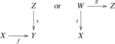
  with s or t is in S, we can complete it to a commutative diagram

  

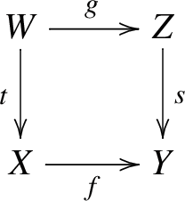
  with t or s is in S, respectively.

• (c) For any morphism $f: X \rightarrow Y$, there exist an object Z and a morphism $s: Y \rightarrow Z$ in S such that $s f = 0$ if and only if there exist an object W and a morphism $t : W \rightarrow X$ in S such that $f t = 0$.

Now we check that the family S of $\mathcal {P}$-isomorphisms satisfies these three conditions.

Proposition 7.9

The family S is a multiplicative system of the category $\mathcal {H}$.

Proof

We have to check the three conditions (a), (b), and (c).

(a) The composite map of two $\mathcal {P}$-isomorphisms is clearly again $\mathcal {P}$-isomorphic, so (a) holds.

(c) Let f be any morphism in $\mathcal {H}$. If there exists either s in S with $s f = 0$ or t in S with $f t = 0$, then we immediately see that f is $\mathcal {P}$-zero, namely $f = 0$ in $\mathcal {H}$. This establishes (c).

(b) We only discuss the case where a diagram $X \overset{f}{\longrightarrow }\ Y \overset{s}{\longleftarrow }\ Z$ is given. The other case can be shown by reversing arrows and dualizing all concepts (replacing surjective by injective and pull-back by push-out).

The basic idea to construct the diagram is to reduce to the case where s is surjective and to make use of the pull-back diagram. However, being surjective is not well-defined in the category $\mathcal {H}$, so for a while we regard the $\mathcal {P}$-isomorphism $s: Z \rightarrow Y$ and a homomorphism $f: X \rightarrow Y$ as morphisms in $\mathcal {C}$ instead of $\mathcal {H}$. Let us take a module $P \in \mathcal {P}$ and a surjective homomorphism $h: P \rightarrow Y$. Then, combining h and s, we can construct $s': Z \oplus P \rightarrow Y$, which is a surjective $\mathcal {P}$-isomorphism. Precisely, writing ${\textrm{pr}}_1: Z \oplus P \rightarrow Z$ and ${\textrm{pr}}_2: Z \oplus P \rightarrow P$ for the projections, we define

$$\begin{aligned} s' = s \circ {\textrm{pr}}_1 + h \circ {\textrm{pr}}_2. \end{aligned}$$

Now we can construct a diagram

where W, t, and $g'$ are defined so that the left square is the pull-back diagram in $\mathcal {C}$. Caution: the right triangle is not necessarily commutative in $\mathcal {C}$.

Since $s'$ is a surjective $\mathcal {P}$-isomorphism, so is t (see Lemma 7.5 and use the isomorphism ${\textrm{Ker}}(t) \simeq {\textrm{Ker}}(s')$). We define $g = {\textrm{pr}}_1 \circ g': W \rightarrow Z$. Then it only remains to show that the right triangle is commutative in $\mathcal {H}$ (not in $\mathcal {C}$). The commutativity can be rephrased as $s' - s \circ {\textrm{pr}}_1: Z \oplus P \rightarrow Y$ is $\mathcal {P}$-zero. By the displayed definition of $s'$, we have $s' - s \circ {\textrm{pr}}_1 = h \circ {\textrm{pr}}_2$, so this morphism factors through the module $P \in \mathcal {P}$. Therefore, this morphism is $\mathcal {P}$-zero. $\square$

Thanks to this proposition, we can define the desired category $\mathcal {D}$ as follows.

Definition 7.10

We define the derived category $\mathcal {D}$ as the localization $\mathcal {D}= \mathcal {H}[S^{-1}]$.

For later use, it is useful to review how to construct the localization. The objects of $\mathcal {H}[S^{-1}]$ are nothing but the objects of $\mathcal {H}$. The set of morphisms in $\mathcal {H}[S^{-1}]$ from X to Y is defined as

$$\begin{aligned} {\textrm{Hom}}_{\mathcal {H}[S^{-1}]}(X, Y) = \varinjlim _{s: X' \rightarrow X} {\textrm{Hom}}_{\mathcal {H}}(X', Y), \end{aligned}$$

where $s: X' \rightarrow X$ runs over morphisms in S, the limit is taken with respect to morphisms $h: X'' \rightarrow X'$ such that $s h = s'$ for $s: X' \rightarrow X$ and $s': X'' \rightarrow X$, and the associated transition map ${\textrm{Hom}}_{\mathcal {H}}(X', Y) \rightarrow {\textrm{Hom}}_{\mathcal {H}}(X'', Y)$ is given by $f \mapsto f h$. Therefore, a morphism in $\mathcal {H}[S^{-1}]$ is represented by $(X', s, f)$, where $X'$ is an object, $s: X' \rightarrow X$ is in S, and $f: X' \rightarrow Y$ is a morphism in $\mathcal {H}$.

The identity morphism in $\mathcal {H}[S^{-1}]$ of X is represented by $(X, {\textrm{id}}_X, {\textrm{id}}_X): X \rightarrow X$. It is easy to see that a morphism $(X', s, f): X \rightarrow X$ also represents the identity morphism if and only if we have $s = f$.

The composition of two morphisms $(X', s, f): X \rightarrow Y$ and $(Y', t, g): Y \rightarrow Z$ is defined as follows. By the property (b), we can find an object $X''$, a morphism $u: X'' \rightarrow X'$ in S, and a morphism $h: X'' \rightarrow Y'$ such that $t h = f u$. Then the composition is defined as $(X'', s u, g h): X \rightarrow Z$. The situation is illustrated by the following diagram

The main and final result of this section is the following.

Theorem 7.11

Let X, Y be modules in $\mathcal {C}$. Then $X \sim Y$ if and only if X and Y are isomorphic in $\mathcal {D}$.

Proof

First assume $X \sim Y$. By Proposition 7.6, we find a module Z and $\mathcal {P}$-isomorphisms $f: Z \rightarrow X$ and $g: Z \rightarrow Y$ (which we may assume to be surjective). By the very construction, f and g become isomorphisms in $\mathcal {D}$, so X is isomorphic to Y in $\mathcal {D}$ via $g f^{-1}$.

The other implication is a little trickier. We assume X and Y to be isomorphic in $\mathcal {D}$. So we have morphisms $(X', s, f): X \rightarrow Y$ and $(Y', t, g): Y \rightarrow X$ such that their composition, both ways, is identity in $\mathcal {D}$.

Let us first consider (s, f) followed by (t, g). Then we may use the above diagram with Z replaced by X. Since the morphism $(X'', s u, g h)$ is to be identity in $\mathcal {D}$, we must have $g h = s u$, so we have gh is in S. In particular, g is onto and h is monic on Ext. (This is abuse of language for saying that these maps induce onto and monic homomorphisms respectively after applying ${\textrm{Ext}}^i(-,M)$ for any $i\ge 0$ and any R-module M). Using the commutative square, we see that the second statement also transfers to give: f is monic on Ext.

Now we reverse the roles. This produces that f is onto on Ext and g is monic on Ext. Taken together, this gives that both f and g are $\mathcal {P}$-isomorphisms. Since s and t were $\mathcal {P}$-isomorphisms, by Proposition 7.6, we may conclude that $X \sim Y$. $\square$

References

Atsuta, M., Kataoka, T.: Fitting ideals of class groups for CM abelian extensions. preprint, arXiv:2104.14765 (2021)
Cornacchia, P., Greither, C.: Fitting ideals of Class groups of real fields with prime power conductor. J. Number Theor. 73, 459–471 (1998)
Curtis, C. W., Reiner, I.: Methods of representation theory. Vol. I. Wiley Classics Library. John Wiley & Sons, Inc., New York, 1990. With applications to finite groups and orders, Reprint of the 1981 original, A Wiley-Interscience Publication
Dasgupta, S., Kakde, M.: On the Brumer-Stark conjecture. Annals Math. 197(1), 289–388 (2023)
Dieterich, E.: Lattices over group rings of cyclic \(p\)-groups and generalized factor space categories. J. Lond. Math. Soc. (2), 31(3), 407–424 (1985)
Greither, C.: Determining Fitting ideals of minus class groups via the equivariant Tamagawa number conjecture. Compos. Math. 143(6), 1399–1426 (2007)
Jannsen, U.: Iwasawa modules up to isomorphism. In: Algebraic number theory, vol. 17 of Adv. Stud. Pure Math., pp. 171–207. Academic Press, Boston, MA (1989)
Kaplansky, I.: Commutative Rings. Allyn and Bacon, Boston (1970)
Kataoka, T.: Fitting invariants in equivariant Iwasawa theory. In: Development of Iwasawa Theory–the Centennial of K. Iwasawa’s Birth, vol.86 of Adv. Stud. Pure Math., pp.413–465, Math. Soc. Japan, Tokyo (2020)
Kurihara, M.: Notes on the dual of the ideal class groups of CM-fields. J. Théor. Nombres Bordeaux 33 (3.2), 971–996 (2021)
Acknowledgements
The second-named author acknowledges support by JSPS KAKENHI Grant Number 19J00763. Both authors would like to thank the anonymous referee for an extremely insightful and detailed report, containing many useful suggestions.
Funding
Open Access funding enabled and organized by Projekt DEAL. The authors affirm that there was no funding on C. Greither’s side involved in the elaboration of this paper. T. Kataoka was funded by JSPS KAKENHI Grant Number 19J00763 (as stated in the acknowledgments).
Author information
Authors and Affiliations
Corresponding author
Ethics declarations
Conflict of interest
The authors declare that there is no conflict of interest of any kind in the context of this paper.
Data Availability
During the work on this publication, no data sets were generated, used or analyzed. Thus, there is no need for a link to a data repository.
Additional information
Publisher's Note
Springer Nature remains neutral with regard to jurisdictional claims in published maps and institutional affiliations.
Rights and permissions
Open Access This article is licensed under a Creative Commons Attribution 4.0 International License, which permits use, sharing, adaptation, distribution and reproduction in any medium or format, as long as you give appropriate credit to the original author(s) and the source, provide a link to the Creative Commons licence, and indicate if changes were made. The images or other third party material in this article are included in the article’s Creative Commons licence, unless indicated otherwise in a credit line to the material. If material is not included in the article’s Creative Commons licence and your intended use is not permitted by statutory regulation or exceeds the permitted use, you will need to obtain permission directly from the copyright holder. To view a copy of this licence, visit http://creativecommons.org/licenses/by/4.0/.
About this article
Cite this article
Greither, C., Kataoka, T. Fitting ideals and various notions of equivalence for modules. manuscripta math. 173, 259–291 (2024). https://doi.org/10.1007/s00229-022-01448-1
Received:
Accepted:
Published:
Issue Date:
DOI: https://doi.org/10.1007/s00229-022-01448-1