
Abstract
In this paper we study the extension of Painlevé/gauge theory correspondence to circular quivers by focusing on the special case of SU(2) \({\mathcal {N}}=2^*\) theory. We show that the Nekrasov–Okounkov partition function of this gauge theory provides an explicit combinatorial expression and a Fredholm determinant formula for the tau-function describing isomonodromic deformations of \(SL_2\) flat connections on the one-punctured torus. This is achieved by reformulating the Riemann–Hilbert problem associated to the latter in terms of chiral conformal blocks of a free-fermionic algebra. This viewpoint provides the exact solution of the renormalization group flow of the SU(2) \({\mathcal {N}}=2^*\) theory on self-dual \(\Omega \)-background and, in the Seiberg–Witten limit, an elegant relation between the IR and UV gauge couplings.


Notes
In the following we will only deal with so-called regular singularities, i.e. simple poles. This means that the solution to the Riemann–Hilbert problem will involve monodromies but not Stokes’ jumps, and the corresponding gauge theory is conformal in the UV. Stokes’ phenomena occur when L(z) has higher order poles, and the corresponding gauge theory is asymptotically free or at an Argyres–Douglas point.
Subject to the non-resonance condition [40].
Comparing to [8] we change \(\theta _k\rightarrow -\theta _k\).
Fourier transformed block is denoted by \(\langle \ldots \rangle _D\) here, but usually we will omit “D”.
In general, L transforms as a connection, so in the transition functions \(T_A,T_B\) there could be also a nonhomogeneous term. However, these matrices can be chosen so that they are z-independent up to a scalar multiple [55].
Here and below we use the standard Pauli matrices \(\sigma ^x=\begin{pmatrix}0&{}1\\ 1&{}0\end{pmatrix}\), \(\sigma ^y=\begin{pmatrix}0&{}-i\\ i&{}0\end{pmatrix}\), \(\sigma ^z=\begin{pmatrix}1&{}0\\ 0&{}-1\end{pmatrix}\). Bold letters always mean either vectors, or diagonal matrices.
This equation is the isomonodromy deformation equation because it is equivalent to the Lax pair equation

which can be shown, by using Eq. (A.13), to be the zero-curvature compatibility condition of the system
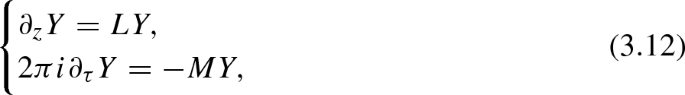
where M is the other matrix of the Lax pair of L:

where \(y(u,z)=\partial _u(u,z)\) .
The factor of i in \(M_A\) comes from the Jacobian of transition from plane to cylinder for a field of dimension \(\frac{1}{4}\).
Recall that \(\det Y(z)=1\), so that the extra U(1) factors \(e^{2\pi i\rho }\) and \(e^{-2\pi i\sigma }\) from the point of view of the linear system are introduced artificially. In fact, they are arbitrary and we can set them to any value, but it turns out to be convenient to keep them arbitrary throughout the computations.
These two shifts mean that we are fermionizing the degenerate fields into fermions which are periodic along both cycles on the torus (in the sense that no additional signs are involved in the computation of monodromies). The shift in \(\sigma \) amounts to the periodicity condition on the cylinder, while that in \(\rho \) is implemented in the operator formalism we are using by an insertion of \((-)^F\) in all our traces.
The precise statement is that to get Nekrasov factors one has to make \(\text {Res }_0 L(z)dz\) of rank 1 by an appropriate U(1) shift. It is the standard AGT trick: see also discussion in the end of Sect. 4.1.
The first case corresponds to \(\text {Res }_{w=1} L(w) dw\sim \text {diag}(m,-m)\), whereas the second one corresponds to \(\text {Res }_{w=1} L(w)dw\sim \text {diag}(2m,0)\). The second normalization was used in [34].
Such small variations preserve the integrals of motion. There is also another part of the problem: to find slow evolution of the integrals of motion at the time scale \(t\sim \hbar ^{-1}\). The general approach to this problem, which gives rise to Whitham equations, is given in [71]. Relation of this approach to our general solution of the non-autonomous problem still has to be uncovered.
Note that all the quantities in the isomonodromic setting are dimensionless, being measured in Omega-background units.
Similar results were recently obtained in the case of SU(2) \(N_f=4\) superconformal gauge theory in [74].
Comparing to [11] we changed here the sign of the fusion matrix, so that for \(m=0\) braiding is trivial.
This algorithm is not optimal for the computation of non-trivial coefficients: as we will see later, it gives a lot of zero terms in the dual partition functions.
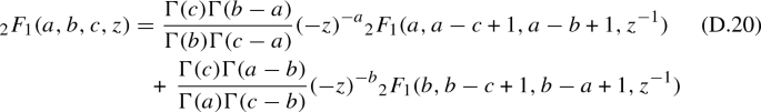
To do this we use connection formula for hypergeometric function
Note this is the same redefinition of (4.5), if \(\eta =4\pi \beta '\), which we will see is the case.


References
Donagi, R., Witten, E.: Supersymmetric Yang–Mills theory and integrable systems. Nucl. Phys. B 460, 299 (1996). arXiv:hep-th/9510101
Nekrasov, N.A., Shatashvili, S.L.: Quantization of integrable systems and four dimensional gauge theories. In: Proceedings of 16th International Congress on Mathematical Physics (ICMP09), Prague, Czech Republic, August 3–8, 2009, pp. 265–289 (2009). arXiv:0908.4052
Alday, L.F., Gaiotto, D., Tachikawa, Y.: Liouville correlation functions from four-dimensional Gauge theories. Lett. Math. Phys. 91, 167 (2010). arXiv:0906.3219
Nekrasov, N.: BPS/CFT correspondence: non-perturbative Dyson–Schwinger equations and qq-characters. JHEP 03, 181 (2016). arXiv:1512.05388
Bonelli, G., Lisovyy, O., Maruyoshi, K., Sciarappa, A., Tanzini, A.: On Painlevé/gauge theory correspondence. Lett. Math. Phys. 107, 2359 (2017). arXiv:1612.06235
Gamayun, O., Iorgov, N., Lisovyy, O.: Conformal field theory of Painlevé VI. JHEP 10, 038 (2012). arXiv:1207.0787
Gamayun, O., Iorgov, N., Lisovyy, O.: How instanton combinatorics solves Painlevé VI, V and IIIs. J. Phys. A 46, 335203 (2013). arXiv:1302.1832
Iorgov, N., Lisovyy, O., Teschner, J.: Isomonodromic tau-functions from Liouville conformal blocks. Commun. Math. Phys. 336, 671 (2015). arXiv:1401.6104
Bershtein, M.A., Shchechkin, A.I.: Bilinear equations on Painlevé \(\tau \) functions from CFT. Commun. Math. Phys. 339, 1021 (2015). arXiv:1406.3008
Gavrylenko, P.G., Marshakov, A.V.: Free fermions, W-algebras and isomonodromic deformations. Theor. Math. Phys. 187, 649 (2016). arXiv:1605.04554
Gavrylenko, P., Iorgov, N., Lisovyy, O.: Higher rank isomonodromic deformations and \(W\)-algebras. arXiv:1801.09608
Nagoya, H.: Irregular conformal blocks, with an application to the fifth and fourth Painlevé equations. J. Math. Phys. 56, 123505 (2015). arXiv:1505.02398
Nagoya, H.: Remarks on irregular conformal blocks and Painlevé III and II tau functions. In: The Proceedings of ’Meeting for Study of Number Theory, Hopf Algebras and Related Topics, Toyama, 12–15 February 2017’ (2018). arXiv:1804.04782
Bershtein, M.A., Shchechkin, A.I.: q-deformed Painlevé \(\tau \) function and q-deformed conformal blocks. J. Phys. A 50, 085202 (2017). arXiv:1608.02566
Bershtein, M., Gavrylenko, P., Marshakov, A.: Cluster integrable systems \(q\)-Painlevé equations and their quantization. JHEP 02, 077 (2018). arXiv:1711.02063
Bershtein, M., Gavrylenko, P., Marshakov, A.: Cluster Toda chains and Nekrasov functions. arXiv:1804.10145
Mironov, A., Morozov, A.: q-Painlevé equation from Virasoro constraints. Phys. Lett. B 785, 207 (2018). arXiv:1708.07479
Jimbo, M., Nagoya, H., Sakai, H.: CFT approach to the q-Painlevé VI equation. J. Integr. Syst. 2 (2017). arXiv:1706.01940
Matsuhira, Y., Nagoya, H.: Combinatorial expressions for the tau functions of \(q\)-Painlevé V and III equations. arXiv:1811.03285
Grassi, A., Hatsuda, Y., Marino, M.: Topological strings from quantum mechanics. Ann. Henri Poincare 17, 3177 (2016). arXiv:1410.3382
Bonelli, G., Grassi, A., Tanzini, A.: Seiberg Witten theory as a Fermi gas. Lett. Math. Phys. 107, 1 (2017). arXiv:1603.01174
Bonelli, G., Grassi, A., Tanzini, A.: New results in \(\cal{N}=2\) theories from non-perturbative string. Ann. Henri Poincare 19, 743 (2018). arXiv:1704.01517
Bonelli, G., Grassi, A. Tanzini, A.: Quantum curves and \(q\)-deformed Painlevé equations. arXiv:1710.11603
Grassi, A., Gu, J.: Argyres–Douglas theories, Painlevé II and quantum mechanics. arXiv:1803.02320
Gaiotto, D.: N=2 dualities. JHEP 08, 034 (2012). arXiv:0904.2715
Gaiotto, D., Moore, G.W., Neitzke, A.: Wall-crossing, Hitchin Systems, and the WKB Approximation. arXiv:0907.3987
Bonelli, G., Tanzini, A.: Hitchin systems, N=2 gauge theories and W-gravity. Phys. Lett. B 691, 111 (2010). arXiv:0909.4031
Teschner, J.: Quantization of the Hitchin moduli spaces, Liouville theory, and the geometric Langlands correspondence I. Adv. Theor. Math. Phys. 15, 471 (2011). arXiv:1005.2846
Bonelli, G., Maruyoshi, K., Tanzini, A.: Quantum Hitchin systems via \({\beta }\)-deformed matrix models. Commun. Math. Phys. 358, 1041 (2018). arXiv:1104.4016
Teschner, J., Vartanov, G.S.: Supersymmetric gauge theories, quantization of \(\cal{M}_{\rm flat}\), and conformal field theory. Adv. Theor. Math. Phys. 19, 1 (2015). arXiv:1302.3778
Gaiotto, D.: Asymptotically free \(\cal{N} = 2\) theories and irregular conformal blocks. J. Phys. Conf. Ser. 462, 012014 (2013). arXiv:0908.0307
Marshakov, A., Mironov, A., Morozov, A.: On non-conformal limit of the AGT relations. Phys. Lett. B 682, 125 (2009). arXiv:0909.2052
Bonelli, G., Maruyoshi, K., Tanzini, A.: Wild quiver gauge theories. JHEP 02, 031 (2012). arXiv:1112.1691
Nekrasov, N., Okounkov, A.: Seiberg–Witten theory and random partitions. Prog. Math. 244, 525 (2006). arXiv:hep-th/0306238
Bonelli, G., Del Monte, F., Gavrylenko, P., Tanzini, A.: Circular quiver gauge theories, isomonodromic deformations and \(W_N\) fermions on the torus. arXiv:1909.07990
Gorsky, A., Krichever, I., Marshakov, A., Mironov, A., Morozov, A.: Integrability and Seiberg–Witten exact solution. Phys. Lett. B 355, 466 (1995). arXiv:hep-th/9505035
Levin, A.M., Olshanetsky, M.A.: Classical limit of the Knizhnik–Zamolodchikov–Bernard equations as hierarchy of isomondromic deformations: free fields approach. arXiv:hep-th/9709207
Edelstein, J.D., Gomez-Reino, M., Marino, M., Mas, J.: N=2 supersymmetric gauge theories with massive hypermultiplets and the Whitham hierarchy. Nucl. Phys. B 574, 587 (2000). arXiv:hep-th/9911115
Jimbo, M.: Monodromy problem and the boundary condition for some Painlevé equations. Publ. Res. Inst. Math. Sci. 18, 1137 (1982)
Jimbo, M., Miwa, T., Ueno, aK: Monodromy preserving deformations of linear differential equations with rational coefficients 1. Physica D2, 306 (1981)
Fokas, A., Its, A., Kapaev, A., Kapaev, A., Novokshenov, V., Novokshenov, V.: Painlevé Transcendents: The Riemann–Hilbert Approach. American Mathematical Society, Mathematical Surveys and Monographs (2006)
Conte, R.: The Painlevé Property: One Century Later. CRM Series in Mathematical Physics. Springer, New York (2011)
Jimbo, M., Miwa, T., Ueno, aK: Monodromy preserving deformations of linear differential equations with rational coefficients. 2. Physica D2, 407 (1982)
Malgrange, B.: Sur les déformations isomonodromiques. i. singularités régulières. Cours de l’institut Fourier 17, 1 (1982)
Bertola, M.: The dependence on the monodromy data of the isomonodromic tau function. Commun. Math. Phys. 294, 539 (2010). arXiv:0902.4716
Sato, M., Miwa, T., Jimbo, M.: Holonomic quantum fields I. Publ. Res. Inst. Math. Sci. 14, 223 (1978)
Sato, M., Miwa, T., Jimbo, M.: Holonomic quantum fields. II. Publ. Res. Inst. Math. Sci. 15, 201 (1979)
Sato, M., Miwa, T., Jimbo, M.: Holonomic quantum fields III. Publ. Res. Inst. Math. Sci. 15, 577 (1979)
Sato, M., Miwa, T., Jimbo, M.: Holonomic quantum fields. IV. Publ. Res. Inst. Math. Sci. 15, 871 (1979)
Sato, M., Miwa, T., Jimbo, M.: Holonomic quantum fields. V. Publ. Res. Inst. Math. Sci. 16, 531 (1980)
Gavrylenko, P.: Isomonodromic \(\tau \)-functions and \(W_{N}\) conformal blocks. JHEP 09, 167 (2015). arXiv:1505.00259
Moore, G., Seiberg, N.: Classical and quantum conformal field theory. Commun. Math. Phys. 123, 177 (1989)
Drukker, N., Gomis, J., Okuda, T., Teschner, J.: Gauge theory loop operators and Liouville theory. JHEP 02, 057 (2010). arXiv:0909.1105
Okuda, T.: Line operators in supersymmetric gauge theories and the 2d–4d relation. In: Teschner, J. (ed.) New Dualities of Supersymmetric Gauge Theories, pp. 195–222 (2016). arXiv:1412.7126
Levin, A., Olshanetsky, M., Zotov, A.: Classification of isomonodromy problems on elliptic curves. Russ. Math. Surv. 69, 35 (2014). arXiv:1311.4498
Levin, A.M., Olshanetsky, M.A., Zotov, A.: Hitchin systems-symplectic hecke correspondence and two-dimensional version. Commun. Math. Phys. 236, 93 (2003). arXiv:nlin/0110045
Levin, A., Olshanetsky, M.: Hierarchies of isomonodromic deformations and hitchin systems. Transl. Am. Math. Soc. Ser. 2(191), 223 (1999)
Takasaki, K.: Elliptic Calogero–Moser systems and isomonodromic deformations. J. Math. Phys. 40, 5787 (1999)
D’Hoker, E., Phong, D.H.: Calogero–Moser systems in SU(N) Seiberg–Witten theory. Nucl. Phys. B 513, 405 (1998). arXiv:hep-th/9709053
D’Hoker, E., Phong, D.H.: Lectures on supersymmetric Yang–Mills theory and integrable systems. Theoretical physics at the end of the twentieth century. In: Proceedings, Summer School, Banff, Canada, June 27–July 10, 1999, pp. 1–125 (1999). arXiv:hep-th/9912271
D’Hoker, E., Krichever, I.M., Phong, D.H.: Seiberg–Witten theory, symplectic forms, and Hamiltonian theory of solitons. Conf. Proc. C0208124, 124 (2002). arXiv:hep-th/0212313
Gavrylenko, P., Lisovyy, O.: Fredholm determinant and Nekrasov sum representations of isomonodromic tau functions. Commun. Math. Phys. 363, 1 (2018). arXiv:1608.00958
Cafasso, M., Gavrylenko, P., Lisovyy, O.: Tau functions as Widom constants. arXiv:1712.08546
Krichever, I.M.: Elliptic solutions of the Kadomtsev–Petviashvili equation and integrable systems of particles. Funct. Anal. Appl. 14, 282 (1980)
Gaiotto, D.: Surface operators in N = 2 4d gauge theories. JHEP 11, 090 (2012). arXiv:0911.1316
Alday, L.F., Gaiotto, D., Gukov, S., Tachikawa, Y., Verlinde, H.: Loop and surface operators in N=2 gauge theory and Liouville modular geometry. JHEP 01, 113 (2010). arXiv:0909.0945
Nekrasov, N., Rosly, A., Shatashvili, S.: Darboux coordinates, Yang–Yang functional, and gauge theory. Nucl. Phys. Proc. Suppl. 216, 69 (2011). arXiv:1103.3919
Aganagic, M., Dijkgraaf, R., Klemm, A., Marino, M., Vafa, C.: Topological strings and integrable hierarchies. Commun. Math. Phys. 261, 451 (2006). arXiv:hep-th/0312085
Dijkgraaf, R., Hollands, L., Sulkowski, P., Vafa, C.: Supersymmetric gauge theories, intersecting branes and free fermions. JHEP 02, 106 (2008). arXiv:0709.4446
Dijkgraaf, R., Hollands, L., Sulkowski, P.: Quantum curves and D-modules. JHEP 11, 047 (2009). arXiv:0810.4157
Krichever, I.: Isomonodromy equations on algebraic curves, canonical transformations and Whitham equations. arXiv:hep-th/0112096
Gavrilov, L., Perelomov, A.M.: On the explicit solutions of the elliptic Calogero system. J. Math. Phys. 40, 6339 (1999). arXiv:solv-int/9905011
Billó, M., Frau, M., Fucito, F., Lerda, A., Morales, J.F.: S-duality and the prepotential in \( \cal{N}={2}^{\star } \) theories (I): the ADE algebras. JHEP 11, 024 (2015). arXiv:1507.07709
Coman, I., Pomoni, E., Teschner, J.: From quantum curves to topological string partition functions. arXiv:1811.01978
Nakajima, H., Yoshioka, K.: Instanton counting on blowup. 1. Invent. Math. 162, 313 (2005). arXiv:math/0306198
Di Francesco, P., Mathieu, P., Senechal, D.: Conformal Field Theory, Graduate Texts in Contemporary Physics. Springer, New York (1997). https://doi.org/10.1007/978-1-4612-2256-9
Alexandrov, A., Zabrodin, A.: Free fermions and tau-functions. J. Geom. Phys. 67, 37 (2013). arXiv:1212.6049
Acknowledgements
We would like to thank M. Bershtein, H. Desiraju, A. Grassi, I. Krichever, K. Maruyoshi, and F. Morales for their interest in this work and for the numerous discussions. We would also like to thank the organizers of the workshops “Supersymmetric Quantum Field Theories in the Non-perturbative Regime” at GGI, Florence, and “Tau Functions of Integrable Systems and Their Applications” at BIRS, Banff, where part of the work was done. The work of GB and FDM is supported by INFN via Iniziativa Specifica ST&FI. The work of PG was carried out within the HSE University Basic Research Program and funded by the Russian Academic Excellence Project ’5–100’. The results of Sect. 3 were obtained under the support of Russian science foundation within the grant 19-11-00275. PG is also a Young Russian Mathematics award winner and would like to thank its sponsors and jury. The work of AT is supported by INFN via Iniziativa Specifica GAST and PRIN project “Geometria delle varietá algebriche”. The work of GB is supported by the PRIN project “Non-perturbative Aspects Of Gauge Theories And Strings”.
Author information
Authors and Affiliations
Corresponding author
Additional information
Communicated by N. Nekrasov.
Publisher's Note
Springer Nature remains neutral with regard to jurisdictional claims in published maps and institutional affiliations.
Appendices
Elliptic and Theta Functions
For elliptic and theta functions we use the notations of [76]. Our torus has periods \((1,\tau ) \), and the theta function that we use are
where
A prime denotes a derivative with respect to z, and when the theta function or its derivatives are evaluated at \(z=0\), we simply denote it by \(\theta _\nu (\tau )\) or \(\theta _1'(\tau )\), e.t.c. Transformations of \(\theta _1\) under elliptic transformations are
In the main text we use also Weierstrass \(\wp \) and \(\zeta \). \(\wp \) is a doubly periodic function with a single double pole at \(z=0\), that can be written in terms of \(\theta _1\) as
where
Weierstrass’ \(\zeta \) function is minus the primitive of \(\wp \). It has only one simple pole at \(z=0\), and is quasi-elliptic:
Finally, we use Dedekind’s \(\eta \) function, defined as
It is related to the function \(\theta _1\) by
Because of the periodicities (A.3), the elliptic transformations of the Lamé function
are given by
The product of Lamé functions satisfies the following identities:
where \(y(u,z)=\partial _ux(u,z)\), that are used in computing the isomonodromic Hamiltonian \(H_\tau \) from the Lax matrix. Further, to show that the zero-curvature Eq. (3.11) is the compatibility condition for the system (3.12), one has to use the property
The following theta-function identities are used in the study of the autonomous limit:
Fusion and Braiding of Degenerate Fields
In this paper monodromies of the fundamental solution have been computed by braiding and fusion of degenerate fields with Virasoro primaries. Fusion matrices linearly relate different sets of blocks, and analytic continuation of a conformal block along any arbitrary contour can be decomposed in elementary braiding and fusion rules [52] (Fig. 4).

Braiding of a degenerate field and a primary
In this paper we only need the following braiding move, that corresponds to the following analytic continuation operation on the matrix elementsFootnote 17:
where \(\gamma _y\cdot z\) is the analytic continuation of the degenerate field along a contour going around y in the positive direction, on the sphere from zero to infinity. F is the fusion matrix, that with our normalization conventions takes the form
Periodicity of the Tau Functions
Equation (3.14) is invariant under the transformation \(Q\mapsto Q+\frac{n}{2} +\frac{\tau k}{2}\), where \(k,n\in {\mathbb {Z}}\). We denote this transformation by \(\delta _{\frac{n}{2},\frac{k}{2}}\). One might ask the following question: what are the transformation properties of the tau function and dual partition functions under \(\delta _{\frac{n}{2},\frac{k}{2}}\)?
The tau function after the transformation is defined by
Therefore
Using now (3.55) we compute transformations of \(Z_0^D\), \(Z_{1/2}^D\):
In this way we see that the dual partition functions have much better behaviour than the tau function \(\mathcal T\). As we will see later in Appendix D, such shifts of parameters correspond to simple shifts of the initial data:
Therefore transformations of the dual partition functions look as follows:
Therefore we can conclude that \(C_{\frac{n}{2},\frac{k}{2}}=e^{-i\eta \frac{k}{2}}\), so \(\delta _{\frac{n}{2},\frac{k}{2}}\mathcal T=q^{k^2/4}e^{ik(2\pi Q-\frac{\eta }{2})}\mathcal T\).
Asymptotic Calculation of the Tau Function
1.1 Algorithm of computations
We start from the following ansatz for the solution of the non-autonomous Calogero equation:
Series expansion of \(\wp (z|\tau )+2\eta _1(\tau )=-\partial _z^2\log \theta _1(z|\tau )\) looks as follows:
Rewrite now Eq. (3.14) using last two formulas and introducing notation \(s=e^{2\pi i(\alpha \tau +\beta )}\). We also introduce single formal parameter of expansion \(\epsilon \) in the following way: \(q\mapsto q\cdot \epsilon ^2\), \(s\mapsto s\cdot \sqrt{\epsilon }\).
One can see that powers of \(\epsilon \) in the r.h.s. are at least one, therefore higher-order coefficients \(c_{n,k}\) become functions of the lower-order ones, and thus equation can be solved order-by-order starting from \(c_{0,0}=0\)Footnote 18.
After this is done, we need to compute the logarithm of the isomonodromic tau function:
Then we compute the two dual partition functions:
1.2 Results
We solved the equation asymptotically up to \(\epsilon ^6\).
Important information about the function \(f(q,s)=\sum f_{n,k}q^n s^{2k}\) is encoded in the list of non-zero coefficients \(f_{n,k}\): we will denote such coefficients by points (k, n) in the integer plane (sometimes it will be shifted by some fractional numbers which we neglect). We call the set of such points support of the function f.
First we show the support of the solution X(q, s) in Fig. 5. In this picture the gray region contains all coefficients that were computed in the asymptotic expansion. Dotted lines show monomials with the same order of \(\epsilon \). The full support is bounded from below by the lines \(n=0\) and \(n=-k\).

Support of X(q, s)
The first few terms of the expansion look as follows:
The support of the dual partition functions is shown in Fig. 6.

Support of \(Z_{0}^D\) (left) and of \(Z_{1/2}^D\) (right).
We see that some non-trivial cancellation happened and a lot of coefficients that naively might be non-zero (denoted by small dots) actually vanish.
Values of the first non-trivial coefficients are given by
We also found experimentally that normalized values of all other non-trivial coefficients can be given in terms of a single function, which will be identified with the toric conformal block:
Namely, the ratios of coefficients are
We see that the latter formula is in complete agreement with (1.2) if \(\mathcal B\) is a conformal block, so we check that it actually coincides with the AGT formula
where Nekrasov factors are given by
1.3 Asymptotic computation of monodromies
At the moment we have two different parameterization: one in terms of \((\alpha ,\beta )\), initial data of the equation, and another in terms of the monodromy data \((a,\eta )\). We need to know the explicit identification between them. To compute this identification we use the fact that the evolution is isomonodromic, so monodromies can be computed in the limit \(\tau \rightarrow +i\infty \).
One can take just the first term of expansion until it becomes smaller than the first correction. This occurs when \(\sin \pi z\approx e^{2 \pi i\tau }\sin {3\pi z}\), so for \(z=\pm \tau \). We will choose two copies of the A-cycle with \(\mathrm{Im} z=\pm \mathrm{Im} \tau /2\) and work in the region between them. So for all computations to be consistent we need to have \(-1/4<\mathrm{Re}\alpha <1/4\) (one can easily overcome this constraint taking more terms of expansion). Also convergence of the series (D.1) requires \(\alpha >0\). So for simplicity we just take \(\alpha \) to have a sufficiently small positive real part.
Our approximation for x is then
The first terms of the expansion of Q look as
The leading behavior of the connection matrix is
Further expanding up to first order in \(e^{4\pi i\alpha \tau }\) we get
One may notice that there is an equality
where
This equality is a reminiscence of the isomonodromic deformation Eq. (3.12). The solution of the linear system in the region \(z\sim \frac{\tau }{2}\) is given by
Now we compute the analytic continuation of this solution to the region \(z\sim -\frac{\tau }{2}\) along imaginary line \(\mathrm{Re} z=1/2\)Footnote 19:
We wish to compute B-cycle monodromy. Its defining relation is
Using (D.21) we get
We write this expression down keeping only the first orders:
By using also the relation
we can then express \(M_B\) as
We see that to our precision \(M_B\) is actually constant when \(\tau \rightarrow i\infty \), its value is given by
To compare this with the monodromy matrix (3.28) computed by braiding we now change normalization
where
The new monodromy is
Corresponding A-cycle monodromy is clearly given by the formula
These monodromies are related to those computed from CFT (3.28) by a conjugation with the matrix
We can in fact check explicitly that
after we made the identification
1.4 Identification of parameters
One may check that the two asymptotic expansions have the following forms:
Where the structure constants are given by explicit formula
We may check, in particular, that \(C_0=C_{-\frac{1}{2}}=1\), which is consistent with experimental results. We also see that after the redefinitionFootnote 20
Experimentally found tau functions may be rewritten as
where
Again, comparing with expressions (3.55) we find \(a=\alpha \), \(\eta =4\pi \beta '\), consistently with what we found in the asymptotic computation of the monodromy matrices.
A Self-consistency Check
In this appendix we compute the derivative with respect to \(\tau \) of the conformal block, using the generalized Wick’s theorem, and provide a consistency check for the relation 3.32 between free fermion CFT and the linear system 3.4. Namely, we compute
We then note that the derivative of any correlator with respect to the modular parameter \(\tau \) can be realized by an integral over the A-cycle of an insertion of the energy-momentum tensor T(z):
Further, we can use the explicit expression of the free fermion energy-momentum tensor
where \(:\ :\) denotes regular part of the OPE. Then,
Here we added a total derivative to T(z) since it does not change correlator. Now we can compute this expression using the generalized Wick theorem [77]. The second term cancels the one containing pairing between \({\bar{\psi }}_\alpha (w)\) and \(\psi _\beta (y)\). So finally we get only
Comparing (E.1) with (E.5) and using (3.12) we get the identity
We can plug in the explicit expression for L, M and see that the relation will hold iff the following relations are satisfied:
To find the r.h.s. we need to compute two integrals:
\(I_1\) and \(\partial _w I_1\) contribute to diagonal elements, whereas \(I_2\) defines off-diagonal ones.
First we consider the integral over the boundary of the cut torus:
The function inside the integral is not periodic under \(z\rightarrow z+\tau \), but rather acquires a phase \(e^{-2\pi i\epsilon }\). If we take the combination of two contour integrals over A-cycles shifted by \(\tau \) in the opposite directions, they enter with opposite signs times the quasi-periodicity:
On the other hand, this integral can be computed by residues:
Now we take a limit \(\epsilon =0\):
By plugging this result in (E.7) we see that it is satisfied. The second integral can be computed in the same manner, noting that the integrand now has quasi-periodicity \(e^{2\pi i\epsilon }\):
The expansion of this integral up to the first order yields \(I_2\):
because of which (E.8) is satisfied.
Other Determinantal Formulas
We report in this appendix some further identities that can be derived from the Fredholm determinant expression (4.10), that we recall here for convenience:
Notice that \(\left. K\right| _{\rho \ \mapsto \rho +1/2}=-K\). Combining this observation with (3.51) and with periodicity properties of theta functions we find
where we put \(\gamma =0\) to simplify the formulas. For arbitrary \(\gamma \) everything is the same.
Another option is to substitute \(\rho =\frac{1}{4}\) and \(\rho =\frac{1}{4}+\frac{\tau }{2}\) into (3.51) in order to cancel each of the two theta functions:
Rights and permissions
About this article

Cite this article
Bonelli, G., Del Monte, F., Gavrylenko, P. et al. \({\mathcal {N}}\) = \(2^*\) Gauge Theory, Free Fermions on the Torus and Painlevé VI. Commun. Math. Phys. 377, 1381–1419 (2020). https://doi.org/10.1007/s00220-020-03743-y
Received:
Accepted:
Published:
Issue Date:
DOI: https://doi.org/10.1007/s00220-020-03743-y