How Much Delocalisation is Needed for an Enhanced Area Law of the Entanglement Entropy?

Abstract

We consider the random dimer model in one space dimension with Bernoulli disorder. For sufficiently small disorder, we show that the entanglement entropy exhibits at least a logarithmically enhanced area law if the Fermi energy coincides with a critical energy of the model where the localisation length diverges.

Appendix A. On the proof of Theorem 3.4

Theorem 3.4 contains slight improvements of results from [JSBS03], which are necessary to deduce our main result. For us it is vital to control the quantity C in Theorem 3.4 in the limit $v\searrow 0$ which is not done in [JSBS03]. Therefore we repeat some arguments of [JSBS03] in this appendix and keep track of the constants. Again, we assume $v \in \;]0,2[$ and we restrict ourselves to the case $E_{F}=0$, the case of the other critical energy $E_{F}=v$ being analogous.

Given $V \in \{0,1\}$ and $E\in {\mathbb {R}}$, we define the single-step transfer matrix by

$$\begin{aligned} W_V(E):=\left( \begin{array}{@{}cc@{}} vV-E &{} -1 \\ 1&{}0 \end{array}\right) \in {\mathbb {R}}^{2\times 2}. \end{aligned}$$

(A.1)

The (multi-step) transfer matrix

$$\begin{aligned} W^\omega (E;y,x) := \left\{ \begin{array}{@{}cl@{}} W_{V^\omega (y-1)}(E)\cdots W_{V^\omega (x)}(E) &{}\quad \text {if }x<y, \\ 1_{2\times 2} &{}\quad \text {if }x=y, \end{array}\right. \end{aligned}$$

(A.2)

relates the solution of the discrete Schrödinger equation (3.7) at different sites

$$\begin{aligned} W_{V^{\omega }(x)}(E;y,x)\left( \begin{array}{@{}c@{}} \phi ^\omega _E(x) \\ \phi ^\omega _E(x-1) \end{array}\right) =\left( \begin{array}{@{}c@{}} \phi ^\omega _E(y)\\ \phi ^\omega _E(y-1) \end{array}\right) , \end{aligned}$$

(A.3)

where $x \leqslant y$. In our model, the single-dimer transfer matrix

$$\begin{aligned} D_{V}(E):=\big (W_{V}(E)\big )^2 \end{aligned}$$

(A.4)

and its similarity transform

$$\begin{aligned} T_{V}(E):= M^{-1}_vD_{V}(E)M_v =: \left( \begin{array}{@{}cc@{}} \overline{a_V(E)} &{} b_V(E) \\ \overline{b_V(E)} &{} a_V(E) \end{array}\right) \end{aligned}$$

(A.5)

with entries $a_{V}(E), b_{V}(E) \in {\mathbb {C}}$ are of great relevance. Here, the change of basis in ${\mathbb {C}}^{2}$ induced by

$$\begin{aligned} M_v:=m_{v}\left( \begin{array}{@{}cc@{}} \frac{1}{2}\left( v - \mathrm{i}\sqrt{4-v^2}\right) &{}\frac{1}{2}\left( v + \mathrm{i} \sqrt{4-v^2}\right) \\ 1&{}1 \end{array}\right) \end{aligned}$$

(A.6)

simultaneously diagonalises $D_{0}(0)$ and $D_{v}(0)$, i.e. $T_{0}(0)=-1_{2\times 2}$ and $T_{v}(0)$ are both diagonal. The real parameter $m_{v}>0$ is chosen such that $|\det M_{v}| =1$. We remark that for every $w\in {\mathbb {R}}^{2}$ there exists $z\in {\mathbb {C}}$ such that

$$\begin{aligned} M_{v}^{-1} w = \left( \begin{array}{@{}c@{}} z \\ {\overline{z}} \end{array}\right) . \end{aligned}$$

(A.7)

In analogy to (A.2), we define the modified (multi-step) dimer transfer matrix as

$$\begin{aligned} T^\omega (E;y,x) := \left\{ \begin{array}{c@{\quad }l} T_{V^{\omega }(y-2)}(E)\cdots T_{V^{\omega }(x)}(E) &{}\text {if }x<y, \\ 1_{2\times 2} &{} \text {if }x=y, \end{array}\right. \end{aligned}$$

(A.8)

where $x,y\in 2{\mathbb {Z}}$.

For later usage we state the Taylor expansions of the entries of $T_{V}(E)$ as $E\searrow 0$

$$\begin{aligned} \begin{aligned} a_0(E)&=-1 - E \;\frac{2\mathrm{i}}{\sqrt{4-v^2}}+{\mathcal {O}}(E^2),\\ a_1(E)&=-1+\frac{v^2}{2} + \mathrm{i} \;\frac{v}{2} \;\sqrt{4-v^2} - E \;\Big (v+\mathrm{i}\;\frac{2-v^2}{\sqrt{4-v^2}}\Big ) +{\mathcal {O}}(E^2),\\ b_0(E)&=\frac{Ev}{2}\Big (-1 +\mathrm{i}\;\frac{v}{\sqrt{4-v^2}}\Big )+{\mathcal {O}}(E^2),\\ b_1(E)&=-b_0(E)+{\mathcal {O}}(E^2).\end{aligned} \end{aligned}$$

(A.9)

Lemma A.1

(Cf. (42) in [JSBS03]). Given $\theta \in [0,2\pi [$ , let $e_\theta :=\frac{1}{\sqrt{2}}({{\,\mathrm{e}\,}}^{-\mathrm{i}\theta },{{\,\mathrm{e}\,}}^{\mathrm{i}\theta })^T$. For all $v\in \;]0,2[$ , $V\in \{0,1\}$ and all $E\in {\mathbb {R}}$ there exists maps $\Theta _V:\;[0,2\pi [\; \rightarrow {\mathbb {R}}$ and $\rho _V:\;[0,2\pi [\;\rightarrow \;]0,\infty [\,$ such that

$$\begin{aligned} T_{V}(E) e_\theta = \rho _V(\theta ) \, e_{\Theta _V(\theta )} \end{aligned}$$

(A.10)

for all $\theta \in [0,2\pi [$ . Furthermore, we have

$$\begin{aligned} \rho ^2_V(\theta )=1+2|b_V(E)|^2+2\mathrm{Re}\big (a_V(E)b_V(E){{\,\mathrm{e}\,}}^{2\mathrm{i}\theta }\big ). \end{aligned}$$

(A.11)

Proof

The form of $T_{V}(E)$ in (A.5) implies that for every non-zero $w_z:=(z,{{\overline{z}}})^T$, $z\in {\mathbb {C}}\backslash \{0\}$ there exists $\zeta \in {\mathbb {C}}\backslash \{0\}$ such that $T_{V}(E) w_{z} = w_{\zeta }$. Since $w_{\zeta }= \rho e_\Theta$ for a unique $\rho >0$ and $\Theta \in [0,2\pi [\,$, the first part of the lemma follows. The equality (A.11) is verified by a direct computation. $\quad \square$

In the following lemma, which is a modification of (49) in [JSBS03], we use the notation $|\pmb \cdot |$ for the Euclidean norm on ${\mathbb {C}}^{2}$.

Lemma A.2

Let $v\in \;]0,2[\,$, $L\in {\mathbb {N}}$, $E\in [-2,2]$, $\omega \in \Omega$ and $x,y\in \Gamma _{L}$ with $x\leqslant y$.

• (i) Then there exists a constant $c_v \in \;]0,\infty [$ , which depends only on v and obeys

  $$\begin{aligned} \lim _{v\searrow 0}c_v=0, \end{aligned}$$

  (A.12)

  such that for all unit vectors $w\in {\mathbb {R}}^2$, $|w|=1$, there is an angle $\xi _w\in [0,2\pi [$ such that

  $$\begin{aligned} \ln \big (|W^\omega (E;x,-L)w|^{2}\big ) \in 2E \sum _{k=k_0}^{k_1-1} \mathrm{Re}\big ( d_{V^\omega (2k)}{{\,\mathrm{e}\,}}^{2\mathrm{i}\vartheta _k}\big ) +{\mathcal {O}}(E^2L) + c_{v} [-1,1] \end{aligned}$$

  (A.13)

  with $d_V:= {a_{V}}(0) b_{V}'(0)$ for $V\in \{0,1\}$ and where

  $$\begin{aligned} k_0:=\min \{k\in {\mathbb {Z}}:-L\leqslant 2k\}, \qquad k_1:=\max \{k:2k\leqslant x\}, \end{aligned}$$

  (A.14)

  $\vartheta _{k_0}:=\xi _w$ and $\vartheta _{k+1}=\Theta _{V^\omega (2k)}(\vartheta _k)$ for all $k\in \{k_0,\ldots ,k_1-1\}$. The ${\mathcal {O}}(E^2L)$-term in (A.13) has no further dependencies except on the model parameters.

• (ii) Let $\{w_1,w_2\}$ be an orthonormal basis of ${\mathbb {R}}^2$. Then

  $$\begin{aligned} \Vert W^\omega (E;y,x)\Vert \leqslant 2\max _{w\in \{w_1,w_2\}}\max _{z\in \Gamma _L}|W^\omega (E;z,-L)w|^2. \end{aligned}$$

  (A.15)

Proof

• (i) For all $x\in \Gamma _L$ we have

  $$\begin{aligned} W^\omega (E;x,-L)=W^\omega (E;x,2k_1)M_v T^\omega (E;2k_1,2k_0)M_v^{-1} W^\omega (E;2k_0,-L). \end{aligned}$$

  (A.16)

  For $w\in {\mathbb {R}}^2$, $|w|=1$, let the angle $\xi _w\in [0,2\pi [$ be given as the unique solution of

  $$\begin{aligned} e_{\xi _w}=M_v^{-1} W^\omega (E;2k_0,-L)w/|M_v^{-1} W^\omega (E;2k_0,-L)w|. \end{aligned}$$

  (A.17)

  We claim that

  $$\begin{aligned} \ln |W^\omega (E;x,-L)w|^2 \in \sum _{k=k_0}^{k_1-1}\ln \big (\rho _{V^\omega (2k)}(\vartheta _k)^{2}\big ) + c_v [-1,1] \end{aligned}$$

  (A.18)

  with

  $$\begin{aligned} c_v:= 4\ln \big (\Vert M_v\Vert \big ) + 4 \max _{E\in [-2,2]}\max _{V\in \{0,1\}}\ln \Vert W_{V}(E)\Vert >0. \end{aligned}$$

  (A.19)

  To see the validity of (A.18), we iterate Lemma A.1 and conclude

  $$\begin{aligned} |W^\omega (E;x,-L)w|&= |W^\omega (E;x,2k_{1}) M_{v}e_{\vartheta _{k_{1}}}| \prod _{k=k_0}^{k_1-1} \rho _{V^\omega (2k)}(\vartheta _k) \nonumber \\&\qquad \times |M_v^{-1} W^\omega (E;2k_0,-L)w|. \end{aligned}$$

  (A.20)

  Furthermore, we note that

  $$\begin{aligned} \Vert A^{-1}\Vert = \Vert A\Vert \qquad \text {and} \qquad \frac{1}{\Vert A\Vert } \leqslant |Aw| \leqslant \Vert A\Vert \end{aligned}$$

  (A.21)

  hold for any complex $2\times 2$-matrix A with $|\det A| =1$ and any $w\in {\mathbb {C}}^{2}$ with $|w|=1$. Applying this to the first and last factor on the right-hand side of (A.20), yields (A.18).

  The estimate (A.13) now follows from (A.11) and a Taylor expansion in the energy E, using (A.9). Since $\Vert W_V(E)\Vert ,\, \Vert M_v\Vert \rightarrow 1$ as $v\rightarrow 0$ for every $E\in [-2,2]$ and $V\in \{0,1\}$, we conclude (A.12) from (A.19).

• (ii) For all $x,\;y\in \Gamma _L$ we have

  $$\begin{aligned} \Vert W^\omega (E;y,x)\Vert \leqslant \Vert W^\omega (E;y,-L)\Vert \Vert W^\omega (E;x,-L)^{-1}\Vert \leqslant \max _{z\in \Gamma _L}\Vert W^\omega (E;z,-L)\Vert ^2, \end{aligned}$$

  (A.22)

  where we used the equality of norms in (A.21). The claim follows from the observation that for any $2\times 2$ matrix

  $$\begin{aligned} \Vert A\Vert ^2\leqslant 2\max _{w\in \{w_1,w_2\}}\Vert Aw\Vert ^2. \end{aligned}$$

  (A.23)

$\square$

The next lemma accounts for a perturbation in energy and is a variation of [DT03, Lemma 2.1] or [Sim96, Thm. 2J].

Lemma A.3

Let $E,\varepsilon \in {\mathbb {R}}$, $\omega \in \Omega$, $L\in {\mathbb {N}}$ and $G_{E}^{\omega }:=\max _{x,y\in \Gamma _L, x<y}\Vert W^\omega (E;y,x)\Vert$. Then, we have for all $x\in \Gamma _L$ and all $w\in {\mathbb {R}}^2$ with $|w|=1$ the estimate

$$\begin{aligned} |W^\omega (E+\varepsilon ;x,-L)w|^{2} \in |W^\omega (E;x,-L)w|^{2} + (G_{E}^{\omega })^{2} \big ({{\,\mathrm{e}\,}}^{4L|\varepsilon |G_{E}^{\omega }} - 1\big ) \;[-1,1] . \end{aligned}$$

(A.24)

Proof

For $V\in \{0,1\}$ and $E,\varepsilon \in {\mathbb {R}}$ we observe

(A.25)

and expand $W^\omega (E+\varepsilon ;x,-L)$ in powers of $\varepsilon$. For the upper bound, this leads to the estimate

$$\begin{aligned} |W^\omega (E+\varepsilon ;x,-L)w|&\leqslant |W^\omega (E;x,-L)w| + G_{E}^{\omega } \max _{x\in \Gamma _L}\sum _{j=1}^{x+L} \genfrac(){0.0pt}1{x+L}{j} \; (|\varepsilon | G_{E}^{\omega })^j \nonumber \\&\leqslant |W^\omega (E;x,-L)w| + G_{E}^{\omega } \sum _{j=1}^{|\Gamma _L|} \frac{\big (|\Gamma _L||\varepsilon | G_{E}^{\omega }\big )^j}{j!}\nonumber \\&\leqslant |W^\omega (E;x,-L)w| + G_{E}^{\omega } \big ({{\,\mathrm{e}\,}}^{2L|\varepsilon |G_{E}^{\omega }} - 1\big ) \end{aligned}$$

(A.26)

for all $x\in \Gamma _L$ and all unit vectors $w\in {\mathbb {R}}^{2}$. For the lower bound, we use the inverse triangle inequality to estimate the expansion in $\varepsilon$ according to

$$\begin{aligned} |W^\omega (E+\varepsilon ;x,-L)w|&\geqslant |W^\omega (E;x,-L)w| - G_{E}^{\omega } \max _{x\in \Gamma _L}\sum _{j=1}^{x+L} \genfrac(){0.0pt}1{x+L}{j}\;(|\varepsilon | G_{E}^{\omega })^j \nonumber \\&\geqslant |W^\omega (E;x,-L)w| - G_{E}^{\omega } \big ({{\,\mathrm{e}\,}}^{2L|\varepsilon |G_{E}^{\omega }} - 1\big ) \end{aligned}$$

(A.27)

for all $x\in \Gamma _L$ and all unit vectors $w\in {\mathbb {R}}^{2}$. We note that for any $a,b,c \geqslant 0$, the two-sided estimate $a \in b+ c \, [-1,1]$ implies $a^{2} \in b^{2}+ c(2b+c) \, [-1,1]$. In our case, we have $b:=|W^\omega (E;x,-L)w| \leqslant G_{E}^{\omega }$, which implies the claim. $\quad \square$

For convenience we quote [JSBS03, Thm. 6] in our notation and note that the assumption $|\langle {{\,\mathrm{e}\,}}^{2\mathrm{i} \eta _{\pm }}\rangle | < 1$ there is always fulfilled in the dimer model considered in this paper.

Theorem A.4

([JSBS03, Thm. 6]). For $L\in {\mathbb {N}}$, $\alpha >0$, $\theta \in [0,2\pi [$ and $E\in {\mathcal {W}}_{L}$ let

$$\begin{aligned} \Omega _L(\alpha ,E,\theta ):=\Big \{\omega \in \Omega :\;\exists \, k_1\in \tfrac{1}{2}\Gamma _L \cap {\mathbb {Z}}\text { such that } \Big |\sum _{k=k_0}^{k_1}d_{V^\omega (2k)}{{\,\mathrm{e}\,}}^{2\mathrm{i}\vartheta _k}\Big |\geqslant L^{\alpha +\frac{1}{2}}\Big \}, \end{aligned}$$

(A.28)

with $d_{V}$, $k_0$ and $\vartheta _k$ defined as in Lemma A.2(i) with $\vartheta _{k_0}=\theta$. Then there exists quantities $C_1,\;C_2>0$, depending only on $\alpha$ and the model parameters, such that

$$\begin{aligned} {\mathbb {P}}\big (\Omega _L(\alpha ,E,\theta )\big )\leqslant C_1 {{\,\mathrm{e}\,}}^{-C_2L^\alpha }. \end{aligned}$$

(A.29)

Lemma A.5

Let $v\in \;]0,2[\,$. For all $\alpha >0$ there exists $L_0\in {\mathbb {N}}$ such that for all $L\geqslant L_0$ there exists a measurable subset $\Omega _L(\alpha )\subseteq \Omega$ and a constant $c>0$ such that

$$\begin{aligned} {\mathbb {P}}\big (\Omega _L(\alpha )\big )\leqslant {{\,\mathrm{e}\,}}^{-cL^{\alpha /2}} \end{aligned}$$

(A.30)

and such that for all $\omega \in \big (\Omega _L(\alpha )\big )^c$, ${E \in {\mathcal {W}}_{L}}$ and ${x\in \Gamma _L}$

$$\begin{aligned} \Big |W^\omega (E;x,-L) \Big (\begin{array}{@{}c@{}} 1 \\ 0 \end{array} \Big ) \Big |^2 \in [ {{\,\mathrm{e}\,}}^{-3c_v}, {{\,\mathrm{e}\,}}^{3c_v}], \end{aligned}$$

(A.31)

where the constant $c_{v}$ is given by Lemma A.2(i), see (A.19).

Proof

Let $w_1:=(1,0)^{T}$ and $w_2:=(0,1)^{T}$. In view of (A.17), we define a set of modified Prüfer angles

$$\begin{aligned} \Xi {:=}\Big \{\xi {\in }[0,2\pi [\,:\;\exists W\in \{1_{2\times 2}, W_{0}(E), W_{1}(E)\} ,w{\in }\{w_1,w_2\}\text { with } e_{\xi } =\frac{M_v^{-1} Ww}{|M_v^{-1} Ww|}\Big \} \end{aligned}$$

(A.32)

with cardinality $|\Xi | \leqslant 6$. Let

$$\begin{aligned} \Omega _L(\alpha ,E):=\bigcup _{\theta \in \Xi }\Omega _L(\alpha /2,E,\theta ). \end{aligned}$$

(A.33)

Hence, ${\mathbb {P}}(\Omega _L(\alpha ,E))\leqslant 6C_1{{\,\mathrm{e}\,}}^{-C_2L^{\alpha /2}}$ by Theorem A.4, and for all $E\in {\mathcal {W}}_{L}$ and $\omega \in (\Omega _L(\alpha ,E))^c$ the estimate (A.13) yields

$$\begin{aligned} \ln \big (|W^\omega (E;x,-L)w|^{2}\big ) \in {\mathcal {O}}(E^2L) + \big (2E L^{1/2+\alpha /2} + c_{v}\big ) \; [-1,1] \end{aligned}$$

(A.34)

for all $x\in \Gamma _{L}$ and $w\in \{ w_{1}, w_{2}\}$. Hence there exists $L_0^\prime >0$ such that for all $L\geqslant L_0^\prime$, all $E\in {\mathcal {W}}_{L}$, all $\omega \in (\Omega _L(\alpha ,E))^c$, all $x\in \Gamma _{L}$ and $w\in \{w_{1},w_{2}\}$, we have

$$\begin{aligned} \ln \big (|W^\omega (E;x,-L)w|^2\big ) \in 2c_v \, [-1,1]. \end{aligned}$$

(A.35)

The upper bound in (A.35) and Lemma A.2(ii) imply for the quantity $G_{E}^{\omega }$ in Lemma A.3

$$\begin{aligned} G_{E}^{\omega }=\max _{x,y\in \Gamma _L, x<y} \Vert W^\omega (E;y,x)\Vert \leqslant 2 {{\,\mathrm{e}\,}}^{2c_v} \end{aligned}$$

(A.36)

for all $\omega \in (\Omega _L(\alpha ,E))^c$. We define

$$\begin{aligned} \Omega _L(\alpha ):=\bigcup _{\begin{array}{c} n \in {\mathbb {Z}}: \\ n/L^{2} \in {\mathcal {W}}_{L} \end{array}}\Omega _L(\alpha ,n/L^2). \end{aligned}$$

(A.37)

Hence there exists $L_0^{\prime \prime } \geqslant L_{0}'$ and $c>0$ such that for all $L\geqslant L_0^{\prime \prime }$ we have

$$\begin{aligned} {\mathbb {P}}\big [\Omega _L(\alpha ) \big ] \leqslant 18L^{3/2}C_1{{\,\mathrm{e}\,}}^{-C_2L^{\alpha /2}}\leqslant {{\,\mathrm{e}\,}}^{-cL^{\alpha /2}}. \end{aligned}$$

(A.38)

Now, we consider $\omega \in (\Omega _L(\alpha ))^c$ arbitrary and $n\in {\mathbb {Z}}$ arbitrary such that $E_{n} :=n/L^2 \in {\mathcal {W}}_{L}$ and apply Lemma A.3, (A.35) and (A.36) with $E_{n}$, $w=w_{1}$ and any $|\varepsilon | \leqslant L^{-2}$. This gives

$$\begin{aligned} |W^\omega (E;x,-L)w_{1}|^{2}&\in |W^\omega (E_{n};x,-L)w_{1}|^{2} + 4 {{\,\mathrm{e}\,}}^{4c_{v}}\big (\exp \{4{{\,\mathrm{e}\,}}^{2c_{v}}/L\} -1 \big ) \; [-1,1] \nonumber \\&\subseteq [{{\,\mathrm{e}\,}}^{-2c_{v}},e^{2c_{v}}] + 4 {{\,\mathrm{e}\,}}^{4c_{v}}\big (\exp \{4{{\,\mathrm{e}\,}}^{2c_{v}}/L\} -1 \big ) \; [-1,1] \end{aligned}$$

(A.39)

for all $x\in \Gamma _{L}$ and all $E\in D_{n}:= E_{n} + L^{-2} [-1,1]$. Since

$$\begin{aligned} {\mathcal {W}}_{L} \subseteq \bigcup _{n \in {\mathbb {Z}}:\; E_{n}\in {\mathcal {W}}_{L}} D_n \end{aligned}$$

(A.40)

there exists $L_0 \geqslant L_0^{\prime \prime }$ such that for all $L \geqslant L_0$, all $\omega \in (\Omega _L(\alpha ))^c$, all $E\in {\mathcal {W}}_{L}$ and all $x\in \Gamma _{L}$ we have

$$\begin{aligned} |W^\omega (E;x,-L)w_1|^2 \in {{\,\mathrm{e}\,}}^{3c_v} \, [-1,1]. \end{aligned}$$

(A.41)

$\square$

Proof of Theorem 3.4

• (i) Let us first proof (3.12). For every $L\in {\mathbb {N}}$, $x\in \Gamma _L$, $E\in {\mathbb {R}}$ and $\omega \in \Omega$, we infer from (3.7) that

  $$\begin{aligned} r_{x}^\omega (E)^2 = \phi ^\omega _E(x)^2+\phi ^\omega _E(x-1)^2 = \Big |W^\omega (E;x,-L) \Big (\begin{array}{@{}c@{}} 1 \\ 0 \end{array} \Big )\Big |^2 /(R^{\omega }_{E})^2, \end{aligned}$$

  (A.42)

  with the normalisation

  $$\begin{aligned} (R^{\omega }_{E})^2 :=\sum _{k=0}^{L-1}\Big |W^\omega (E;-L+1+2k,-L) \Big (\begin{array}{@{}c@{}} 1 \\ 0 \end{array} \Big )\Big |^2. \end{aligned}$$

  (A.43)

  Given $\alpha >0$, Lemma A.5 provides the existence of a minimal length $L_{0}\in {\mathbb {N}}$ such that for all $L \geqslant L_0$, $\omega \in (\Omega _L(\alpha ))^c$, $x\in \Gamma _{L}$ and $E\in {\mathcal {W}}_{L}$, the two-sided estimate

  $$\begin{aligned} (R^{\omega }_{E})^2 \in [L{{\,\mathrm{e}\,}}^{-3c_v},L{{\,\mathrm{e}\,}}^{3c_v}] \end{aligned}$$

  (A.44)

  holds. Thus, (A.44), another application of Lemma A.5 and (A.42) yield (3.12) with the constant

  $$\begin{aligned} C = {{\,\mathrm{e}\,}}^{6c_v}, \end{aligned}$$

  (A.45)

  and (A.12) implies (3.9). To prove the level-spacing estimate (3.11), let $L_{0}$ be as above, $L \geqslant L_0$, $\omega \in (\Omega _L(\alpha ))^c$ and let $E,E'\in {\mathcal {W}}_{L}$ be two adjacent eigenvalues of $H_L^\omega$ with $E<E'$. For $E^{(\prime )}$ to be an eigenvalue, Dirichlet boundary conditions $\phi ^{\omega }_{E^{(\prime )}}(L)=0$ have to be met on the right-hand side of $\Gamma _{L}$, that is, $\theta ^\omega _{L}(E^{(\prime )})\in \pi /2+\pi {\mathbb {Z}}$. Since $\theta ^\omega _{L}$ is a continuous, increasing function with respect to the energy, E and $E'$ are adjacent eigenvalues if and only if the Prüfer-angle difference satisfies $\theta _{L}^\omega (E^\prime )-\theta _{L}^\omega (E) =\pi$. Using (3.19), this can be rewritten as

  $$\begin{aligned} \pi = \int _E^{E^\prime }{\mathrm {d}}\varepsilon \, \frac{\mathrm {d}}{\mathrm {d}\varepsilon } \theta ^\omega _{L}(\varepsilon ) = \int _E^{E^\prime }{\mathrm {d}}\varepsilon \sum _{x=-L}^{L-1} \left( \frac{\phi _\varepsilon ^\omega (x)}{r_L^\omega (\varepsilon )} \right) ^{2} = \int _E^{E^\prime }{\mathrm {d}}\varepsilon \; \frac{1}{\big (r_L^\omega (\varepsilon )\big )^{2}}.\nonumber \\ \end{aligned}$$

  (A.46)

  The eigenfunction estimate (3.12) does not apply directly to $r_L^\omega (\varepsilon )$ for $\varepsilon \in {\mathcal {W}}_{L}$, but only after an additional iteration with the transfer matrix

  $$\begin{aligned} \big (r_L^\omega (\varepsilon )\big )^{2} = \Big | W_{V^{\omega }(L-1)}(\varepsilon ) \Big (\begin{array}{@{}c@{}} \cos \theta ^{\omega }_{L-1}(\varepsilon ) \\ \sin \theta ^{\omega }_{L-1}(\varepsilon ) \end{array} \Big )\Big |^{2} \big (r_{L-1}^\omega (\varepsilon )\big )^{2}. \end{aligned}$$

  (A.47)

  We already have $\big (r_{L-1}^\omega (\varepsilon )\big )^{2} \in L^{-1} [C^{-1},C]$ for every $\omega \in (\Omega _L(\alpha ))^c$ by (3.12). Since $\max _{V\in \{0,1\}} \Vert W_{V}(\varepsilon )\Vert \leqslant {{\,\mathrm{e}\,}}^{c_{v}/4} \leqslant C$ uniformly in $\varepsilon \in {\mathcal {W}}_{L}$ by (A.19), we deduce from (A.21) that $\big (r_L^\omega (\varepsilon )\big )^{2} \in L^{-1} [C^{-3},C^{3}]$. Inserting this into (A.46), yields

  $$\begin{aligned} E^\prime -E\in \frac{\pi }{L} \; [C^{-3},C^{3}]. \end{aligned}$$

  (A.48)

• (ii) The existence of the density of states ${\mathcal {N}}'(E_{c})$ follows from [JSBS03, Thm. 3], the upper and lower bounds from Dirichlet–Neumann bracketing and the eigenvalue spacing in the critical energy window, as we show now. For $L\in {\mathbb {N}}$ we introduce the restricted Schrödinger operators $H^{\omega ,\,D/N}_L$ with Dirichlet, respectively Neumann, boundary conditions

  

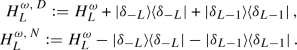  (A.49)

  Their integrated densities of states at energy $E\in {\mathbb {R}}$ are given by

  $$\begin{aligned} {\mathcal {N}}_L^{\omega ,\, D/N}(E):={{\,\mathrm{tr}\,}}\Big \{1_{\leqslant E}\big (H^{\omega ,\,D/N}_L\big )\Big \}. \end{aligned}$$

  (A.50)

  Since $H^{\omega ,\,D/N}_L$ are rank-2-perturbations of $H^\omega _L$, the min-max-principle implies

  $$\begin{aligned} {\mathcal {N}}_L^{\omega ,\, D/N}(E)\in {{\,\mathrm{tr}\,}}\big \{1_{\leqslant E}(H^\omega _L)\big \} + [-2,2]. \end{aligned}$$

  (A.51)

  According to [CL90, p. 312] Dirichlet–Neumann bracketing yields

  $$\begin{aligned} \frac{1}{|\Gamma _L|}{\mathbb {E}}\big [{\mathcal {N}}_L^{D}(E)\big ] \leqslant {\mathcal {N}}(E)\leqslant \frac{1}{|\Gamma _L|}{\mathbb {E}}\big [{\mathcal {N}}_L^{N}(E)\big ] \end{aligned}$$

  (A.52)

  for every $E\in {\mathbb {R}}$ and every $L\in {\mathbb {N}}$. Thus, we conclude from (A.51) and (A.52) that

  $$\begin{aligned} {\mathcal {N}}(E+\varepsilon )-{\mathcal {N}}(E-\varepsilon ) \in \frac{1}{|\Gamma _L|} {\mathbb {E}}\big \{ {{\,\mathrm{tr}\,}}1_{]E-\varepsilon ,E+\varepsilon ]}(H_L)\big \} + \frac{4}{|\Gamma _L|} \; [-1,1] \end{aligned}$$

  (A.53)

  for every $\varepsilon >0$. For fixed $\alpha \in \;]0,1/2[$ let $\varepsilon _L:=L^{-1/2-\alpha }$ be half the width of the critical energy window ${\mathcal {W}}_{L}$ around $E_{c} \in \{0,v\}$. Theorem 3.4(i) provides the existence of a minimal length $L_{0}\in {\mathbb {N}}$ such that for all $L\geqslant L_0$ and all $\omega \in (\Omega _L(\alpha ))^c$ and we have

  $$\begin{aligned} \frac{2\varepsilon L}{\pi C^3} - 1 \leqslant {{\,\mathrm{tr}\,}}\big \{1_{]E_{c}-\varepsilon ,E_{c}+\varepsilon ]}(H^\omega _L)\big \} \leqslant \frac{2\varepsilon C^3 L}{\pi } + 1. \end{aligned}$$

  (A.54)

  The estimates (A.54) and (A.53) imply for $L\geqslant L_{0}$

  $$\begin{aligned} \frac{{\mathcal {N}}(E_{c} + \varepsilon _L) - {\mathcal {N}}(E_{c} - \varepsilon _L)}{2\varepsilon _L}&\in \frac{1}{ 2\varepsilon _L |\Gamma _L|} \; {\mathbb {E}} \big \{ 1_{\Omega _{L}(\alpha )} {{\,\mathrm{tr}\,}}1_{]E_{c}-\varepsilon _{L},E_{c}+\varepsilon _{L}]}(H_L)\big \} \nonumber \\&\quad + \frac{{\mathbb {P}}\big \{\big (\Omega _{L}(\alpha )\big )^{c}\big \}}{2\varepsilon _L |\Gamma _L|} \; \Big [\frac{2\varepsilon _{L}L}{\pi C^{3}}-1, \frac{2\varepsilon _{L} C^3 L}{\pi } + 1\Big ]\nonumber \\&\quad + \frac{2}{\varepsilon _L |\Gamma _L|} \;[-1,1] \nonumber \\&\subseteq \frac{{\mathbb {P}}\big \{\big (\Omega _{L}(\alpha )\big )^{c}\big \} L}{\pi |\Gamma _L|} \; [C^{-3}, C^{3}] \nonumber \\&\quad + \Big ( \frac{{\mathbb {P}}\{\Omega _{L}(\alpha )\}}{2\varepsilon _{L}} + \frac{3}{\varepsilon _{L}|\Gamma _{L}|}\Big ) \; [-1,1]. \end{aligned}$$

  (A.55)

  Now, the claim follows in the limit $L\rightarrow \infty$. $\quad \square$

We finish with an elementary auxiliary result needed in the proof of Theorem 2.1.

Lemma A.6

Let $\gamma \in \;]0,1/2[$ and $\gamma _L:=\lfloor (\gamma +\gamma ^2)L\rfloor -\lfloor \gamma L\rfloor$ for $L\in {\mathbb {N}}$. Then for all $L^\prime \in {\mathbb {N}}$ there exists $L\in {\mathbb {N}}$ such that $L^\prime =\gamma _L$.

Proof

As $\gamma <1$ and $\gamma +\gamma ^2<1$, we infer $\lfloor (\gamma +\gamma ^2)(L+1)\rfloor -\lfloor (\gamma +\gamma ^2)L\rfloor \in \{0,1\}$ and $\lfloor \gamma (L+1)\rfloor -\lfloor \gamma L\rfloor \in \{0,1\}$ for all $L\in {\mathbb {N}}$. Thus, we have $\gamma _{L+1}-\gamma _L\in \{-1,0,1\}$ for all $L\in {\mathbb {N}}$. Together with $\gamma _1=0$ and $\lim _{L\rightarrow \infty }\gamma _L=\infty$, this yields the claim. $\quad \square$

References

Abdul-Rahman, H.: Entanglement of a class of non-Gaussian states in disordered harmonic oscillator systems. J. Math. Phys. 59, 031904–1–17 (2018)
Abdul-Rahman, H., Nachtergaele, B., Sims, R., Stolz, G.: Localization properties of the disordered XY spin chain: a review of mathematical results with an eye toward many-body localization. Ann. Phys. 529, 1600280–1–17 (2017)
Abdul-Rahman, H., Stolz, G.: A uniform area law for the entanglement of eigenstates in the disordered XY chain. J. Math. Phys. 56, 121901–1–25 (2015)
Aizenman, M., Warzel, S.: Random Operators: Disorder Effects on Quantum Spectra and Dynamics, Graduate Studies in Mathematics, vol. 168. American Mathematical Society, Providence (2015)
Amico, L., Fazio, R., Osterloh, A., Vedral, V.: Entanglement in many-body systems. Rev. Mod. Phys. 80, 517–576 (2008)
Beaud, V., Sieber, J., Warzel, S.: Bounds on the bipartite entanglement entropy for oscillator systems with or without disorder, e-print arXiv:1812.09144
Beaud, V., Warzel, S.: Bounds on the entanglement entropy of droplet states in the XXZ spin chain. J. Math. Phys. 59, 012109–1–11 (2018)
Bekenstein, J.D.: Black holes and entropy. Phys. Rev. D 7, 2333–2346 (1973)
Bekenstein, J.D.: Black holes and information theory. Contemp. Phys. 45, 31–43 (2004)
Brandão, F.G.S.L., Horodecki, M.: Exponential decay of correlations implies area law. Commun. Math. Phys. 333, 761–798 (2015)
Calabrese, P., Cardy, J.: Entanglement entropy and conformal field theory. J. Phys. A 42, 504005–1–36 (2009)
Carmona, R., Klein, A., Martinelli, F.: Anderson localization for Bernoulli and other singular potentials. Commun. Math. Phys. 108, 41–66 (1987)
Carmona, R., Lacroix, J.: Spectral Theory of Random Schrödinger Operators. Birkhäuser, Boston (1990)
Damanik, D., Tcheremchantsev, S.: Power-law bounds on transfer matrices and quantum dynamics in one dimension. Commun. Math. Phys. 236, 513–534 (2003)
De Bievre, S., Germinet, F.: Dynamical localization for the random dimer model. J. Stat. Phys. 98, 1135–1148 (2000)
Eisert, J., Cramer, M., Plenio, M.B.: Area laws for the entanglement entropy. Rev. Mod. Phys. 82, 277–306 (2010)
Elgart, A., Pastur, L., Shcherbina, M.: Large block properties of the entanglement entropy of free disordered Fermions. J. Stat. Phys. 166, 1092–1127 (2017)
Fischbacher, C., Stolz, G.: Droplet states in quantum XXZ spin systems on general graphs. J. Math. Phys. 59, 051901–1–28 (2018)
Hastings, M.B.: An area law for one-dimensional quantum systems. J. Stat. Mech. 2007, P08024–1–14 (2007)
Helling, R., Leschke, H., Spitzer, W.: A special case of a conjecture by Widom with implications to fermionic entanglement entropy. Int. Mat. Res. Not. 2011, 1451–1482 (2011)
Horodecki, R., Horodecki, P., Horodecki, M., Horodecki, K.: Quantum entanglement. Rev. Mod. Phys. 81, 865–942 (2009)
Iglói, F., Szatmári, Z., Lin, Y.-C.: Entanglement entropy dynamics of disordered quantum spin chains. Phys. Rev. B 85, 094417–1–8 (2012)
Jin, B.-Q., Korepin, V.E.: Quantum spin chain, Toeplitz determinants and the Fisher–Hartwig conjecture. J. Stat. Phys. 116, 79–95 (2004)
Jitomirskaya, S., Schulz-Baldes, H., Stolz, G.: Delocalization in random polymer models. Commun. Math. Phys. 233, 27–48 (2003)
Kirsch, W.: An invitation to random Schrödinger operators. In: Random Schrödinger operators, Panor. Synthèses, vol. 25, Soc. Math. France, Paris, 2008, pp. 1–119, with an appendix by Frédéric Klopp
Kirsch, W., Lenoble, O., Pastur, L.: On the Mott formula for the ac conductivity and binary correlators in the strong localization regime of disordered systems. J. Phys. A 36, 12157–12180 (2003)
Klich, I.: Lower entropy bounds and particle number fluctuations in a Fermi sea. J. Phys. A 39, L85–L91 (2006)
Laflorencie, N.: Quantum entanglement in condensed matter systems. Phys. Rep. 646, 1–59 (2016)
Leschke, H., Sobolev, A.V., Spitzer, W.: Scaling of Rényi entanglement entropies of the free Fermi-gas ground state: a rigorous proof. Phys. Rev. Lett. 112, 160403–1–5 (2014)
Leschke, H., Sobolev, A.V., Spitzer, W.: Trace formulas for Wiener–Hopf operators with applications to entropies of free fermionic equilibrium states. J. Funct. Anal. 273, 1049–1094 (2017)
Lifshits, I.M., Gredeskul, S.A., Pastur, L.A.: Introduction to the Theory of Disordered Systems. Wiley, New York (1988)
Mott, N.F.: Conduction in non-crystalline systems. I. Localized electronic states in disordered systems. Philos. Mag. 17, 1259–1268 (1968)
Mott, N.F.: Conduction in non-crystalline systems. IV. Anderson localization in a disordered lattice. Philos. Mag. 22, 7–29 (1970)
Movassagh, R., Shor, P.W.: Supercritical entanglement in local systems: counterexample to the area law for quantum matter. Proc. Natl. Acad. Sci. USA 113, 13278–13282 (2016)
Nachtergaele, B., Sims, R., Stolz, G.: An area law for the bipartite entanglement of disordered oscillator systems. J. Math. Phys. 54, 042110–1–24 (2013)
Pastur, L., Figotin, A.: Spectra of Random and Almost-Periodic Operators, Grundlehren der Mathematischen Wissenschaften, vol. 297. Springer, Berlin (1992)
Pastur, L., Slavin, V.: Area law scaling for the entropy of disordered quasifree fermions. Phys. Rev. Lett. 113, 150404–1–5 (2014)
Pastur, L., Slavin, V.: The absence of the selfaveraging property of the entanglement entropy of disordered free fermions in one dimension. J. Stat. Phys. 170, 207–220 (2018)
Peschel, I.: Calculation of reduced density matrices from correlation functions. J. Phys. A 36, L205–L208 (2003)
Pfirsch, B., Sobolev, A.V.: Formulas of Szegő type for the periodic Schrödinger operator. Commun. Math. Phys. 358, 675–704 (2018)
Pouranvari, M., Yang, K.: Maximally entangled mode, metal-insulator transition, and violation of entanglement area law in noninteracting fermion ground states. Phys. Rev. B 89, 115104–1–5 (2014)
Refael, G., Moore, J.E.: Criticality and entanglement in random quantum systems. J. Phys. A 42, 504010–1–31 (2009)
Schmüdgen, K.: Unbounded Self-Adjoint Operators on Hilbert space, Graduate Texts in Mathematics, vol. 265. Springer, Dordrecht (2012)
Simon, B.: Bounded eigenfunctions and absolutely continuous spectra for one-dimensional Schrödinger operators. Proc. Am. Math. Soc. 124, 3361–3369 (1996)
Sobolev, A.V.: Pseudo-Differential Operators with Discontinuous Symbols: Widom’s Conjecture. Memoirs of the American Mathematical Society, vol. 222, no. 1043 (2013)
Sobolev, A.V.: Wiener–Hopf operators in higher dimensions: the Widom conjecture for piece-wise smooth domains. Integr. Equ. Oper. Theory 81, 435–449 (2015)
Stolz, G.: Aspects of the mathematical theory of disordered quantum spin chains, e-print arXiv:1606.01579
Wolf, M.M.: Violation of the entropic area law for fermions. Phys. Rev. Lett. 96, 010404–1–4 (2006)
Author information
Authors and Affiliations
Corresponding author
Additional information
Communicated by L. Erdos.
Publisher's Note
Springer Nature remains neutral with regard to jurisdictional claims in published maps and institutional affiliations.