A Functional Integral Approaches to the Makeenko–Migdal Equations

Abstract

Makeenko and Migdal (Phys Lett B 88(1):135–137, 1979) gave heuristic identities involving the expectation of the product of two Wilson loop functionals associated to splitting a single loop at a self-intersection point. Kazakov and Kostov (Nucl Phys B 176(1):199–215, 1980) reformulated the Makeenko–Migdal equations in the plane case into a form which made rigorous sense. Nevertheless, the first rigorous proof of these equations (and their generalizations) was not given until the fundamental paper of Lévy (2017). Subsequently Driver, Kemp, and Hall Commun. Math. Phys. 351(2), 741–774 (2017) gave a simplified proof of Lévy’s result and then with Driver, Gabriel, Kemp, and Hall Commun. Math. Phys. 352(3), 967–978 (2017) we showed that these simplified proofs extend to the Yang–Mills measure over arbitrary compact surfaces. All of the proofs to date are elementary but tricky exercises in finite dimensional integration by parts. The goal of this article is to give a rigorous functional integral proof of the Makeenko–Migdal equations guided by the original heuristic machinery invented by Makeenko and Migdal. Although this stochastic proof is technically more difficult, it is conceptually clearer and explains “why” the Makeenko–Migdal equations are true. It is hoped that this paper will also serve as an introduction to some of the problems involved in making sense of quantizing Yang–Mill’s fields.

Appendices

Appendix: Connections, Parallel Translation, and Curvature

In this first appendix, we review a few basic facts about covariant derivatives, parallel translation, and curvature. Recall that we have assumed that our compact Lie group is a matrix Lie sub-group of $GL\left( \mathbb {C}^{D}\right) \subset \mathbb {C}^{D\times D}$ for some $D\in \mathbb {N}$.

1.1 Transformation properties

The next result recalls how $g\in \mathcal {G}$ acts on covariant differentiation, parallel translation, and curvature.

Theorem A.1

(Gauge transformed quantities). If $A\in \mathcal {A}$, $g\in \mathcal {G}$, $\ell :\left[ a,b\right] \rightarrow M$ is an absolutely continuous path in M, and $S:\left[ a,b\right] \rightarrow \mathbb {C}^{D}$ (or $S:\left[ a,b\right] \rightarrow \mathbb {C}^{D\times D})$ be a $C^{1}$-function, then

• 1. The operator $\nabla _{t}^{A^{g}}$ is conjugate to $\nabla _{t}^{A}$. More precisely,

  $$\begin{aligned} \nabla _{t}^{A^{g}}S\left( t\right) =g\left( \ell \left( t\right) \right) ^{-1}\nabla _{t}^{A}\left[ g\left( \ell \left( t\right) \right) S\left( t\right) \right] \end{aligned}$$

  (A.1)

  so that $\nabla _{t}^{A^{g}}=M_{g\left( \ell \left( t\right) \right) ^{-1} }\nabla _{t}^{A}M_{g\left( \ell \left( t\right) \right) }$ where $M_{g}$ is used to denote multiplication by g.

• 2. For $t\in \left[ a,b\right]$,

  $$\begin{aligned} //_{t}^{A^{g}}\left( \ell \right) =g\left( \ell \left( t\right) \right) ^{-1}//_{t}^{A}\left( \ell \right) g\left( \ell \left( a\right) \right) . \end{aligned}$$

  (A.2)

• 3. The curvature tensor, $F^{A}$, satisfies,

  $$\begin{aligned} F^{A^{g}}\left\langle v,w\right\rangle =\mathrm {Ad}_{g\left( x\right) ^{-1} }F^{A}\left\langle v,w\right\rangle \text { for all }v,w\in T_{x}M\text { and }x\in M. \end{aligned}$$

  (A.3)

Proof

Equation A.1 follows by direct computation using the product rule and basic calculus. The proof of Eq. (A.2) is now elementary as

$$\begin{aligned} u_{t}:=g\left( \ell \left( t\right) \right) ^{-1}//_{t}^{A}\left( \ell \right) g\left( \ell \left( a\right) \right) \end{aligned}$$

satisfies,

$$\begin{aligned} \nabla _{t}^{A^{g}}u_{t}=g\left( \ell \left( t\right) \right) ^{-1} \nabla _{t}^{A}\left[ g\left( \ell \left( t\right) \right) g\left( \ell \left( t\right) \right) ^{-1}//_{t}^{A}\left( \ell \right) g\left( \ell \left( a\right) \right) \right] =0\text { with }u_{a}=I. \end{aligned}$$

Although the curvature assertion in Eq. (A.3) may be proved by direct calculation, let us give a more conceptual proof which makes use of the fact that curvature is related to the commutator of two covariant derivatives. More precisely, let $\varSigma \left( s,t\right) \in M$ and $S\left( s,t\right) \in \mathbb {C}^{D}$ (or $\mathbb {C}^{D\times D})$ be two $C^{1}$-functions of $\left( s,t\right) \in \mathbb {R}^{2}$ and let

$$\begin{aligned} \nabla _{t}^{A}:=\frac{d}{dt}+A\left( \dot{\varSigma }\left( t,s\right) \right) \quad \text {and}\quad \nabla _{s}^{A}:=\frac{d}{ds}+A\left( \varSigma ^{\prime }\left( t,s\right) \right) . \end{aligned}$$

A straightforward computation, using $\left[ \frac{d}{dt},\frac{d}{ds}\right] =0$ and Cartan’s formula,

$$\begin{aligned} \frac{d}{dt}A\left( \varSigma ^{\prime }\left( t,s\right) \right) -\frac{d}{ds}A\left( \dot{\varSigma }\left( t,s\right) \right) =dA\left( \dot{\varSigma }\left( t,s\right) ,\varSigma ^{\prime }\left( t,s\right) \right) , \end{aligned}$$

shows

$$\begin{aligned} \left[ \nabla _{t}^{A},\nabla _{s}^{A}\right] S\left( s,t\right) =F^{A}\left( \dot{\varSigma }\left( t,s\right) ,\varSigma ^{\prime }\left( t,s\right) \right) S\left( s,t\right) . \end{aligned}$$

(A.4)

Thus it follows that

$$\begin{aligned}&F^{A^{g}}\left( \dot{\varSigma }\left( t,s\right) ,\varSigma ^{\prime }\left( t,s\right) \right) S\left( s,t\right) \\&\quad =\left[ \nabla _{t}^{A^{g} },\nabla _{s}^{A^{g}}\right] S\left( s,t\right) \\&\quad =\left[ M_{g\left( \varSigma \left( s,t\right) \right) ^{-1}}\nabla _{t}^{A}M_{g\left( \varSigma \left( s,t\right) \right) },M_{g\left( \varSigma \left( s,t\right) \right) ^{-1}}\nabla _{s}^{A}M_{g\left( \varSigma \left( s,t\right) \right) }\right] S\left( s,t\right) \\&\quad =M_{g\left( \varSigma \left( s,t\right) \right) ^{-1}}\left[ \nabla _{t}^{A},\nabla _{s}^{A}\right] M_{g\left( \varSigma \left( s,t\right) \right) }S\left( s,t\right) \\&\quad =M_{g\left( \varSigma \left( s,t\right) \right) ^{-1}}F^{A}\left( \dot{\varSigma }\left( t,s\right) ,\varSigma ^{\prime }\left( t,s\right) \right) M_{g\left( \varSigma \left( s,t\right) \right) }S\left( s,t\right) \end{aligned}$$

from which Eq. (A.3) is easily deduced. $\quad \square$

Remark A.2

One more formula connecting covariant differentiation to parallel translation is the identity;

$$\begin{aligned} \nabla _{t}^{A}S=//_{t}^{A}\left( \ell \right) \frac{d}{dt}\left[ //_{t}^{A}\left( \ell \right) ^{-1}S\left( t\right) \right] . \end{aligned}$$

(A.5)

To prove this let $V\left( t\right) :=//_{t}^{A}\left( \ell \right) ^{-1}S\left( t\right)$ so that $S\left( t\right) =//_{t}^{A}\left( \ell \right) V\left( t\right)$. Now apply the product rule and use $\nabla _{t}^{A}//_{t}^{A}\left( \ell \right) =0$ to find,

$$\begin{aligned} \nabla _{t}^{A}S\left( t\right)&=\nabla _{t}^{A}\left[ //_{t}^{A}\left( \ell \right) V\left( t\right) \right] =\left( \frac{d}{dt}+A\left( \dot{\ell }\left( t\right) \right) \right) \left[ //_{t}^{A}\left( \ell \right) V\left( t\right) \right] \\&=\left[ \left( \frac{d}{dt}+A\left( \dot{\ell }\left( t\right) \right) \right) //_{t}^{A}\left( \ell \right) \right] V\left( t\right) +//_{t}^{A}\left( \ell \right) \dot{V}\left( t\right) =//_{t}^{A}\left( \ell \right) \dot{V}\left( t\right) \end{aligned}$$

which is Eq. (A.5).

Proposition A.3

(Connections and diffeomorphisms). Let $\varphi :M\rightarrow M$ be a diffeomorphism of M, $\sigma \in C^{1}\left( \left[ a,b\right] ,M\right)$, and $A\in \mathcal {A}$. Then $F^{\varphi ^{*}A} =\varphi ^{*}F^{A}$ and $//_{t}^{\varphi ^{*}A}\left( \sigma \right) =//_{t}^{A}\left( \varphi \circ \sigma \right)$ for all $a\le t\le b$.

Proof

Using the basic properties of pull backs on forms we have,

$$\begin{aligned} \varphi ^{*}F^{A}=\varphi ^{*}\left[ dA+A\wedge A\right] =d\left[ \varphi ^{*}A\right] +\varphi ^{*}A\wedge \varphi ^{*}A=F^{\varphi ^{*}A}. \end{aligned}$$

For the second assertion we compute,

$$\begin{aligned} 0&=\frac{\nabla }{dt}//_{t}^{A}\left( \varphi \circ \sigma \right) :=\left[ \frac{d}{dt}+A\left\langle \frac{d}{dt}\left( \varphi \circ \sigma \left( t\right) \right) \right\rangle \right] //_{t}^{A}\left( \varphi \circ \sigma \right) \\&=\left[ \frac{d}{dt}+A\left\langle \varphi _{*}\dot{\sigma }\left( t\right) \right\rangle \right] //_{t}^{A}\left( \varphi \circ \sigma \right) =\left[ \frac{d}{dt}+\left( \varphi ^{*}A\right) \left\langle \dot{\sigma }\left( t\right) \right\rangle \right] //_{t}^{A}\left( \varphi \circ \sigma \right) \end{aligned}$$

from which we see that $//_{t}^{A}\left( \varphi \circ \sigma \right)$ satisfies the same differential equation as $//_{t}^{\varphi ^{*}A}\left( \sigma \right)$.

$\square$

Corollary A.4

If $\dim M=2$, $A\in \mathcal {A}$, and $\varphi :M\rightarrow M$ is an area preserving diffeomorphism, then $\left\| F^{\varphi ^{*} A}\right\| ^{2}=\left\| F^{A}\right\| ^{2}$.

Proof

By definition,

$$\begin{aligned} \left\| F^{\varphi ^{*}A}\right\| ^{2}=\int _{M}\left| F^{\varphi ^{*}A}\right| ^{2}d\mathrm{Vol}_{g}=\int _{M}\left| \varphi ^{*}F^{A}\right| ^{2}d\mathrm{Vol}_{g}. \end{aligned}$$

(A.6)

Since $d=2$, if we let $\omega$ denote the (local) Riemannian volume form on M then $F^{A}=f\cdot \omega$ for some $f:M\rightarrow \mathfrak {k.}$ The assumption that $\varphi$ is area preserving means $\varphi ^{*}\omega =\pm \omega$ and therefore,

$$\begin{aligned} \varphi ^{*}F^{A}=f\circ \varphi \cdot \varphi ^{*}\omega =\pm f\circ \varphi \cdot \omega . \end{aligned}$$

As $\omega \left( e_{1},e_{2}\right) =\pm 1$ where $\left\{ e_{1} ,e_{2}\right\}$ is any local orthonormal frame on M, we find

$$\begin{aligned} \left| \varphi ^{*}F^{A}\right| ^{2}=\left| f\circ \varphi \right| ^{2}=\left| F^{A}\right| ^{2}\circ \varphi . \end{aligned}$$

Using this result in Eq. (A.6) gives,

$$\begin{aligned} \left\| F^{\varphi ^{*}A}\right\| ^{2}=\int _{M}\left| F^{A}\right| ^{2}\circ \varphi ~d\mathrm{Vol}_{g}=\int _{M}\left| F^{A}\right| ^{2}~d\mathrm{Vol}_{g} =\left\| F^{A}\right\| ^{2}, \end{aligned}$$

where in the second equality we have the area preserving assumption again, namely that $\varphi _{*}\mathrm{Vol}_{g}=\mathrm{Vol}_{g}$. $\quad \square$

1.2 Differential properties of parallel translation

Proposition A.5

(Connection Comparison). Suppose that A and B are two connection 1-forms, $\ell \in C^{1}\left( \left[ 0,1\right] ,M\right)$, and $k_{t}:=//_{t}^{B}\left( \ell \right) //_{t}^{A}\left( \ell \right) ^{-1}$, then

$$\begin{aligned} \dot{k}_{t}+\left( \mathrm {Ad}_{//_{t}^{A}\left( \ell \right) ^{-1}}\left[ B\left( \dot{\ell }\left( t\right) \right) -A\left( \dot{\ell }\left( t\right) \right) \right] \right) k_{t}=0\text { with }k_{0}=0. \end{aligned}$$

(A.7)

Proof

Since $//_{t}^{B}\left( \ell \right) =//_{t}^{A}\left( \ell \right) k_{t}$, $\nabla _{t}^{B}//_{t}^{B}\left( \ell \right) =0=\nabla _{t} ^{A}//_{t}^{A}\left( \ell \right)$ it follows that

$$\begin{aligned} 0&=\nabla _{t}^{B}//_{t}^{B}\left( \ell \right) =\left( \nabla _{t} ^{B}//_{t}^{A}\left( \ell \right) \right) k_{t}+//_{t}^{A}\left( \ell \right) \dot{k}_{t}\\&=\left( \left[ \nabla _{t}^{B}-\nabla _{t}^{A}\right] //_{t}^{A}\left( \ell \right) \right) k_{t}+//_{t}^{A}\left( \ell \right) \dot{k}_{t}\\&=\left[ B\left( \dot{\ell }\left( t\right) \right) -A\left( \dot{\ell }\left( t\right) \right) \right] //_{t}^{A}\left( \ell \right) k_{t}+//_{t}^{A}\left( \ell \right) \dot{k}_{t} \end{aligned}$$

from which Eq. (A.7) follows. $\quad \square$

Proposition A.6

(Connection Differentiation). If $\eta$ is a $\mathfrak {k}$ -valued one form on M and $\ell \in C^{1}\left( \left[ 0,1\right] ,M\right)$, then

$$\begin{aligned} \partial _{\eta }\left[ A\rightarrow //^{A}\left( \ell \right) \right]&=-//^{A}\left( \ell \right) \int _{0}^{1}\mathrm {Ad}_{//_{t}^{A}\left( \ell \right) ^{-1}}\eta \left( \dot{\ell }\left( t\right) \right) dt \end{aligned}$$

(A.8)

$$\begin{aligned}&=-\left[ \int _{0}^{1}\mathrm {Ad}_{//_{t}^{A}\left( \ell \right) } \eta \left( \dot{\ell }\left( t\right) \right) dt\right] //^{A}\left( \ell \right) . \end{aligned}$$

(A.9)

Proof

First proof. Differentiating the identity, $0=\nabla _{t}^{A+s\eta }//_{t}^{A+s\eta }\left( \ell \right)$ with respect to s gives,

$$\begin{aligned} 0&=\frac{d}{ds}|_{0}\left[ \nabla _{t}^{A+s\eta }//_{t}^{A+s\eta }\left( \ell \right) \right] \\&=\left[ \frac{d}{ds}|_{0}\nabla _{t}^{A+s\eta }\right] //_{t}^{A}\left( \ell \right) +\nabla _{t}^{A}\left[ \frac{d}{ds}|_{0}//_{t}^{A+s\eta }\left( \ell \right) \right] \\&=\eta \left( \dot{\ell }\left( t\right) \right) //_{t}^{A}\left( \ell \right) +\nabla _{t}^{A}\partial _{\eta }//_{t}^{A}\left( \ell \right) \\&=\eta \left( \dot{\ell }\left( t\right) \right) //_{t}^{A}\left( \ell \right) +//_{t}^{A}\left( \ell \right) \frac{d}{dt}\left[ //_{t} ^{A}\left( \ell \right) ^{-1}\partial _{\eta }//_{t}{}^{A}\left( \ell \right) \right] \end{aligned}$$

wherein we have used Eq. (A.5) in the last equality. Multiplying this equation by $//_{t}^{A}\left( \ell \right) ^{-1}$ and then integrating the result easily gives Eq. (A.8) which is equivalent to Eq. (A.9).

Second proof. Letting $B=A+s\eta$ in Proposition A.5 shows $//_{t}^{A+s\eta }\left( \ell \right) =//_{t}^{A}\left( \ell \right) k_{t}^{s}$ where

$$\begin{aligned} \dot{k}_{t}^{s}+s\left( \mathrm {Ad}_{//_{t}^{A}\left( \ell \right) ^{-1} }\eta \left( \dot{\ell }\left( t\right) \right) \right) k_{t}^{s}=0\text { with }k_{0}^{s}=0. \end{aligned}$$

Differentiating this equation with respect to s at $s=0$ while using $k_{t}^{0}=I$ shows

$$\begin{aligned} \frac{d}{ds}|_{0}\dot{k}_{t}^{s}+\mathrm {Ad}_{//_{t}^{A}\left( \ell \right) ^{-1}}\eta \left( \dot{\ell }\left( t\right) \right) =0 \end{aligned}$$

and then integrating this result relative to t shows

$$\begin{aligned} \frac{d}{ds}|_{0}k_{t}^{s}=-\int _{0}^{t}\mathrm {Ad}_{//_{\tau }^{A}\left( \ell \right) ^{-1}}\eta \left( \dot{\ell }\left( \tau \right) \right) d\tau . \end{aligned}$$

Hence it follows that

$$\begin{aligned} \partial _{\eta }\left[ A\rightarrow //_{t}^{A}\left( \ell \right) \right]&=\frac{d}{ds}|_{0}//_{t}^{A+s\eta }\left( \ell \right) =\frac{d}{ds} |_{0}//_{t}^{A}\left( \ell \right) k_{t}^{s}\\&=-//_{t}^{A}\left( \ell \right) \int _{0}^{t}\mathrm {Ad}_{//_{\tau } ^{A}\left( \ell \right) ^{-1}}\eta \left( \dot{\ell }\left( \tau \right) \right) d\tau . \end{aligned}$$

$\square$

Proposition A.7

(Path Differentiation). Suppose $\ell _{s}$ is a one parameter family of curves parametrized by an interval, $\left[ 0,1\right]$ such that $\ell _{s}\left( 0\right)$ is constant independent of s and let $//_{t}^{A}\left( \ell \right)$ denote parallel translation along $\ell _{s}|_{\left[ 0,t\right] }$. Then,

$$\begin{aligned} \frac{\nabla ^{A}}{ds}//_{t}^{A}\left( \ell _{s}\right) =//_{t}^{A}\left( \ell _{s}\right) \int _{0}^{t}\mathrm {Ad}_{//_{\tau }^{A}\left( \ell _{s}\right) ^{-1}}F^{A}\left( \dot{\ell }_{s}\left( \tau \right) ,\ell _{s}^{\prime }\left( \tau \right) \right) d\tau \end{aligned}$$

(A.10)

and, if we further assume that $\ell _{s}\left( 1\right)$ is constant independent of s, then

$$\begin{aligned} \frac{d}{ds}//_{1}^{A}\left( \ell _{s}\right) =//_{1}^{A}\left( \ell _{s}\right) \int _{0}^{1}\mathrm {Ad}_{//_{\tau }^{A}\left( \ell _{s}\right) ^{-1}}F^{A}\left( \dot{\ell }_{s}\left( \tau \right) ,\ell _{s}^{\prime }\left( \tau \right) \right) d\tau . \end{aligned}$$

(A.11)

Equation (A.10) may also be expressed as,

$$\begin{aligned}&\frac{d}{ds} \left[ //_{s}^{A}\left( \ell _{\left( \cdot \right) }\left( t\right) \right) ^{-1}//_{t}^{A}\left( \ell _{s}\right) \right] \nonumber \\&\quad =\left[ //_{s}^{A}\left( \ell _{\left( \cdot \right) }\left( t\right) \right) ^{-1}//_{t}^{A}\left( \ell _{s}\right) \right] \int _{0}^{t}\mathrm {Ad} _{//_{\tau }^{A}\left( \ell _{s}\right) ^{-1}}F^{A}\left( \dot{\ell } _{s}\left( \tau \right) ,\ell _{s}^{\prime }\left( \tau \right) \right) d\tau . \end{aligned}$$

(A.12)

Proof

By Eq. (A.4) and the fact that $\frac{\nabla ^{A}}{dt}//_{t} ^{A}\left( \ell _{s}\right) =0$,

$$\begin{aligned} \frac{\nabla ^{A}}{dt}\frac{\nabla ^{A}}{ds}//_{t}^{A}\left( \ell _{s}\right) =\left[ \frac{\nabla ^{A}}{dt},\frac{\nabla ^{A}}{ds}\right] //_{t} ^{A}\left( \ell _{s}\right) =F^{A}\left( \dot{\ell }_{s}\left( t\right) ,\ell _{s}^{\prime }\left( t\right) \right) //_{t}^{A}\left( \ell _{s}\right) . \end{aligned}$$

By Remark A.2, the last identity may be rewritten as,

$$\begin{aligned} \frac{d}{dt}\left[ //_{t}^{A}\left( \ell \right) ^{-1}\frac{\nabla ^{A}}{ds}//_{t}^{A}\left( \ell _{s}\right) \right] =//_{t}^{A}\left( \ell \right) ^{-1}F^{A}\left( \dot{\ell }\left( t\right) ,\ell _{s}^{\prime }\left( t\right) \right) //_{t}^{A}\left( \ell \right) . \end{aligned}$$

Integrating this equation on t gives Eq. (A.10). If we now assume $\ell _{s}\left( 1\right)$ is constant in s, then

$$\begin{aligned} \frac{\nabla ^{A}}{ds}//_{1}^{A}\left( \ell _{s}\right) =\left( \frac{d}{ds}+A\left\langle \ell _{s}^{\prime }\left( 1\right) \right\rangle \right) //_{1}^{A}\left( \ell _{s}\right) =\frac{d}{ds}//_{1}^{A}\left( \ell _{s}\right) \end{aligned}$$

which combined with Eq. (A.10) at $t=1$ gives Eq. (A.11). $\quad \square$

For more information on Proposition A.7 much more related material to this and the next appendix, see [12, 18].

Homotopy Gauge Fixing of Yang–Mills

The goal of this appendix is to motivate the definition of the Yang–Mills measure as used in this paper. We also wish to give a heuristic argument that the resulting expectations should be invariant under area preserving diffeomorphisms. We begin with a few general results in finite dimensions which we will later apply (illegally) in the infinite dimensional Yang–Mills context. For an interesting general discussion of gauge fixing from a differential form point, as apposed to the more measure theoretic view described in this appendix, see [29, Sect. III]. There is of course a huge physics literature on various methods of gauge fixing which we do not attempt to survey here. However, the interested reader might start with Chapter 13 in [11, Sect. 13.6] or Chapter 15 in [34] and then consult some of the references in [29].

1.1 Group actions and gauges

We will use the following notation throughout this subsection.

Notation B.1

Let $\left( \mathcal {A},\mathcal {G},m,\lambda \right)$ be a quadruple consisting of a smooth manifold, $\mathcal {A}$, a Lie group $\mathcal {G}$, a smooth measure $\left( m\right)$ on $\mathcal {A}$, and a right invariant Haar measure $\left( \lambda \right)$ on $\mathcal {G}$. We assume that there is a given right action of $\mathcal {G}$ on $\mathcal {A}$ and that the measure m is invariant under this right action, i.e. m is invariant under the transformation, $\mathcal {A\ni }A\rightarrow Ag\in \mathcal {A}$ for each $g\in \mathcal {G}$.

Definition B.2

A gauge is a smooth function, $v:\mathcal {A} \rightarrow \mathcal {G}$, such that $v\left( Ag\right) =v\left( A\right) g$ for all $A\in \mathcal {A}$ and $g\in \mathcal {G}$. Associated to v we defined the “projection map,” $\pi _{v} :\mathcal {A}\rightarrow \mathcal {A}$, by $\pi _{v}\left( A\right) :=A\cdot v\left( A\right) ^{-1}$ and let

$$\begin{aligned} \mathcal {A}_{v}:=\pi _{v}\left( \mathcal {A}\right) =\left\{ A\cdot v\left( A\right) ^{-1}:A\in \mathcal {A}\right\} . \end{aligned}$$

Lemma B.3

If $v:\mathcal {A}\rightarrow \mathcal {G}$ is a gauge and $A,B\in \mathcal {A}$, then;

• 1. $\pi _{v}$ is constant on gauge orbits,

• 2. $\pi _{v}\circ \pi _{v}=\pi _{v}$ (i.e. $\pi _{v}|_{\mathcal {A}_{v}}$ is the identity on $\mathcal {A}_{v})$,

• 3. $\mathcal {A}_{v}$ may also be expresses as

  $$\begin{aligned} \mathcal {A}_{v}=\left\{ A\in \mathcal {A}:v\left( A\right) =I\in \mathcal {G}\right\} , \end{aligned}$$

• 4. $\mathcal {A}_{v}$ is an embedded submanifold of $\mathcal {A}$,

• 5. $\pi _{v}\left( A\right) =\pi _{v}\left( B\right)$ iff A and B are in the same $\mathcal {G}$-orbit, and

• 6. the map,

  $$\begin{aligned} \mathcal {A}_{v}\times \mathcal {G}\ni \left( A,g\right) \rightarrow A\cdot g\in \mathcal {A} \end{aligned}$$

  (B.1)

  is as diffeomorphism of smooth manifolds.

Proof

We take each item in turn.

• 1. If $A\in \mathcal {A}$ and $g\in \mathcal {G}$, then

  $$\begin{aligned} \pi _{v}\left( Ag\right) =Ag\cdot v\left( Ag\right) ^{-1}=Ag\cdot \left[ v\left( A\right) g\right] ^{-1}=A\cdot v\left( A\right) ^{-1}=\pi _{v}\left( A\right) \end{aligned}$$

  which shows $\pi _{\nu }$ is constant on $\mathcal {G}$-orbits.

• 2. If $A\in \mathcal {A}$, then A and $\pi _{v}\left( A\right)$ are in the same gauge orbit and hence $\pi _{v}\left( \pi _{v}\left( A\right) \right) =\pi _{v}\left( A\right)$.

• 3. If $A\in \mathcal {A}_{v}$ then $A=\pi _{\nu }\left( A\right) =A\cdot v\left( A\right) ^{-1}$ and therefore,

  $$\begin{aligned} v\left( A\right) =v\left( A\cdot v\left( A\right) ^{-1}\right) =v\left( A\right) \cdot v\left( A\right) ^{-1}=I. \end{aligned}$$

  Conversely if $\nu \left( A\right) =I$, then $\pi _{v}\left( A\right) =A\in \mathcal {A}_{v}$.

• 4. If $A\in \mathcal {A\ }$and $\xi \in \mathrm{Lie}\left( \mathcal {G}\right) =T_{I}\mathcal {G}$, then

  $$\begin{aligned} \frac{d}{dt}|_{0}v\left( Ae^{t\xi }\right) =\frac{d}{dt}|_{0}\left[ v\left( A\right) e^{t\xi }\right] =L_{v\left( A\right) *}\xi \end{aligned}$$

  where the latter expression varies over $T_{v\left( A\right) }G$ as $\xi$ varies over $\mathrm{Lie}\left( \mathcal {G}\right)$. This shows $\nu$ is a submersion and so the level sets of v are all embedded submanifolds, in particular$\mathcal {A}_{v}=v^{-1}\left( \left\{ I\right\} \right)$ is an embedded submanifold.

• 5. The condition that $\pi _{v}\left( A\right) =\pi _{v}\left( B\right)$ is equivalent to $A\cdot v\left( A\right) ^{-1}=B\cdot v\left( B\right) ^{-1}$ which is then equivalent to $B=A\cdot \left[ v\left( A\right) ^{-1}v\left( B\right) \right]$, i.e. B and A are in the same gauge orbit.

• 6. The inverse to the smooth map in Eq. (B.1) is the smooth map, $\mathcal {A}\ni A\rightarrow \left( \pi _{v}\left( A\right) ,v\left( A\right) \right)$. $\quad \square$

Example B.4

(Product groups). Let $\mathcal {G}$ be a Lie group, $N\in \mathbb {N}$, $\mathcal {A}=\mathcal {G}^{N}$, and let $\mathcal {G}$ act on $\mathcal {A}$ on the right by the diagonal action,

$$\begin{aligned} \mathcal {A\times G}\ni \left( \overrightarrow{g},k\right) \rightarrow \overrightarrow{g}\cdot k\in \mathcal {A}\text { where }\left[ \overrightarrow{g}\cdot k\right] _{i}=g_{i}k\text { for }1\le i\le N. \end{aligned}$$

Then $\nu :\mathcal {A}\rightarrow \mathcal {G}$ defined by $v\left( \overrightarrow{g}\right) =g_{1}$ is a gauge. In this case

$$\begin{aligned} \pi _{v}\left( \overrightarrow{g}\right) =\overrightarrow{g}\cdot g_{1} ^{-1}=\left( \begin{array} [c]{c} e\\ g_{2}g_{1}^{-1}\\ \vdots \\ g_{N}g_{1}^{-1} \end{array} \right) \end{aligned}$$

and $\mathcal {A}_{v}=\left\{ e\right\} \times \mathcal {G}^{N-1}$.

Example B.5

Let $\mathcal {A}=\mathbb {R}^{n}$, $\mathcal {G}=\mathbb {R}$, $\xi \in sl\left( n,\mathbb {R}\right)$ such that $\xi _{lk}=0$ if either l or $k=n$ and for $x\in \mathbb {R}^{n}$ (thought of as row vector) and $t\in \mathbb {R}$ let

$$\begin{aligned} x\cdot t:=xe^{t\xi }+te_{n}=\left[ x+te_{n}\right] e^{t\xi }. \end{aligned}$$

Since $e_{n}\xi =0$ we have $e_{n}e^{t\xi }=e_{n}$ and by assumption $e^{t\xi }$ preserves $\mathrm{span}\left( e_{k}\right) _{k<n}$ and hence

$$\begin{aligned} \left( x\cdot t\right) \cdot s=\left( xe^{t\xi }+te_{n}\right) e^{s\xi }+se_{n}=xe^{t\xi }e^{s\xi }+te_{n}+se_{n}=x\cdot \left( t+s\right) . \end{aligned}$$

In this case the projection map, $v\left( x\right) =x_{n}$ is a gauge with

$$\begin{aligned} \pi _{\nu }\left( x\right) =xe^{-x_{n}\xi }-x_{n}e_{n}=\left( \begin{array} [c]{c} x_{1}\\ \vdots \\ x_{n-1}\\ 0 \end{array} \right) e^{-x_{n}\xi }\text { and }\mathcal {A}_{v}=\mathbb {R}^{n-1} \times \left\{ 0\right\} . \end{aligned}$$

Example B.6

Let us specializing Example B.5 to $n=3$ and

$$\begin{aligned} \xi =\left[ \begin{array} [c]{lll} 0 &{}\quad -1 &{}\quad 0\\ 1 &{}\quad 0 &{}\quad 0\\ 0 &{}\quad 0 &{}\quad 0 \end{array} \right] \quad \implies \quad \text { }e^{t\xi }=\left[ \begin{array} [c]{lll} \cos t &{} \quad -\sin t &{}\quad 0\\ \sin t &{} \quad \cos t &{}\quad 0\\ 0 &{} \quad 0 &{} \quad 1 \end{array} \right] . \end{aligned}$$

In this case the gauge orbits are spirals. For example, the gauge orbit of $e_{1}=\left( 1,0,0\right) \in \mathbb {R}^{3}$ is the spiral, $\left\{ e_{1}\cdot t=\left( \cos t,-\sin t,t\right) :\text { }t\in \mathbb {R}\right\} .$

Examples B.5 and B.6 were examples of “affine actions,” which we now define.

Definition B.7

(Affine actions). Assume $\left( \mathcal {A},\mathcal {G}\right)$ as above with $\mathcal {A}$ being a finite dimensional vector space and let $SL\left( \mathcal {A}\right)$ denote the special linear transformations on $\mathcal {A}$. We say the group action of $\mathcal {G}$ on $\mathcal {A}$ is an affine action if it may be written in the form;

$$\begin{aligned} Ag=\rho \left( g^{-1}\right) A+T\left( g\right) \end{aligned}$$

(B.2)

where $\rho :\mathcal {G}\rightarrow SL\left( \mathcal {A}\right)$ is a representation of $\mathcal {G}$ and $T:\mathcal {G}\rightarrow \mathcal {A}$ is a smooth function.

Remark B.8

It is left to the interested reader to verify that $T\left( e\right) =0$ and the pair, $\left( \rho ,T\right)$, must satisfy the “cocycle” condition;

$$\begin{aligned} T\left( gh\right) =\rho \left( h^{-1}\right) T\left( g\right) +T\left( h\right) \text { }\forall ~g,h\in \mathcal {G}. \end{aligned}$$

(B.3)

The key formal example of an affine action is the right action of the restricted gauge group acting on connection one forms as in Eq. (1.1). We will work heuristically with this formal infinite dimensional setup in Sect. B.4 below.

1.2 Disintegration formulas

Proposition B.9

(Disintegration). Let $\left( \mathcal {A},\mathcal {G} ,m,\lambda \right)$ be as in Notation B.1. To each gauge, $v:\mathcal {A}\rightarrow \mathcal {G}$, there exists a unique (smooth) measure $m_{v}$ on $\mathcal {A}_{v}$ such that

$$\begin{aligned} \int _{\mathcal {A}}f\left( A\right) dm\left( A\right) =\int _{\mathcal {A} _{v}}dm_{v}\left( B\right) \int _{\mathcal {G}}d\lambda \left( g\right) f\left( Bg\right) \end{aligned}$$

(B.4)

for all $f:\mathcal {A\rightarrow }\left[ 0,\infty \right]$ measurable.

Proof

Let $\gamma$ be a fixed smooth measure on $\mathcal {A}_{v}$. Since the map in Eq. (B.1) is a diffeomorphism and Haar measure, $\lambda$, is a smooth measure on $\mathcal {G}$, there exists a smooth density, $\mu :\mathcal {A} _{v}\times \mathcal {G}\rightarrow \left( 0,\infty \right)$, such that

$$\begin{aligned} \int _{\mathcal {A}}f\left( A\right) dm\left( A\right) =\int _{\mathcal {A} _{v}}d\gamma \left( B\right) \int _{\mathcal {G}}d\lambda \left( g\right) \mu \left( B,g\right) f\left( Bg\right) \end{aligned}$$

(B.5)

for all $f:\mathcal {A\rightarrow }\left[ 0,\infty \right]$ measurable. Using the invariance of m and $\lambda$ under the right $\mathcal {G}$-actions on $\mathcal {A}$ and $\mathcal {G}$ respectively, if $k\in \mathcal {G}$, then

$$\begin{aligned} \int _{\mathcal {A}}f\left( A\right) dm\left( A\right)&=\int _{\mathcal {A}}f\left( Ak\right) dm\left( A\right) \nonumber \\&=\int _{\mathcal {A}_{v}}d\gamma \left( B\right) \int _{\mathcal {G}} d\lambda \left( g\right) \mu \left( B,g\right) f\left( Bgk\right) \nonumber \\&=\int _{\mathcal {A}_{v}}d\gamma \left( B\right) \int _{\mathcal {G}} d\lambda \left( g\right) \mu \left( B,gk^{-1}\right) f\left( Bg\right) . \end{aligned}$$

(B.6)

Comparing Eqs. (B.5) and (B.6) implies $\mu \left( B,gk^{-1}\right) =\mu \left( B,g\right)$ for all $B\in \mathcal {A}_{v}$ and $g,k\in \mathcal {G}$. Taking $k=g$ shows $\mu \left( B,g\right) =\mu \left( B,e\right)$ and so Eq. (B.4) holds with $dm_{v}\left( B\right) :=\mu \left( B,e\right) d\gamma \left( B\right)$. $\quad \square$

Theorem B.10

(Affine Action Disintegrations). Assume $\left( \mathcal {A} ,\mathcal {G}\right)$ as above with $\mathcal {A}$ being a finite dimensional vector space equipped with an affine action of $\mathcal {G}$ on $\mathcal {A}$, see Definition B.7. Then;

• 1. Lebesgue measure $\left( m\right)$ on $\mathcal {A}$ is invariant under the $\mathcal {G}$-action.

• 2. If $v:\mathcal {A}\rightarrow \mathcal {G}$ is a gauge such that $\mathcal {A}_{v}$ is a linear subspace which is invariant under the action of $\rho$, then the measure $\left( m_{\nu }\right)$ in Proposition B.9 is a Lebesgue measure on $\mathcal {A}_{v}$.

Proof

1. The Jacobian-determinant factor for the change of variables, $B=Ag$, is $\left| \det \rho \left( g^{-1}\right) \right| =1$ and hence the affine transformation $A\rightarrow Ag$ leaves m invariant on $\mathcal {A}$.

2. Let $m_{0}$ be a Lebesgue measure on $\mathcal {A}_{v}$ (i.e. a translation invariant Radon measure on $\mathcal {A}_{v}\mathcal {)}$. The smooth measure $\left( m_{\nu }\right)$ may be expressed as $dm_{\nu }\left( A\right) =\mu \left( A\right) dm_{0}\left( A\right)$ for some smooth density $\mu :\mathcal {A}\rightarrow \left( 0,\infty \right)$. Our goal is to show that $\mu$ is a constant.

According to Proposition B.9, if $f:\mathcal {A}\rightarrow \left[ 0,\infty \right]$ is measurable, then

$$\begin{aligned} \int _{\mathcal {A}}f\left( C\right) dm\left( C\right)&=\int _{\mathcal {A} _{v}}dm_{\nu }\left( A\right) \int _{\mathcal {G}}d\lambda \left( g\right) f\left( A\cdot g\right) \nonumber \\&=\int _{\mathcal {G}}d\lambda \left( g\right) \int _{\mathcal {A}_{v}}dm_{0}\left( A\right) \mu \left( A\right) f\left( A\cdot g\right) . \end{aligned}$$

(B.7)

Let $B\in \mathcal {A}_{v}$ and apply Eq. (B.7) with f replaced by $f\left( \cdot +B\right)$ to find

$$\begin{aligned} \int _{\mathcal {A}}f\left( C+B\right) dm\left( C\right)&=\int _{\mathcal {G}}d\lambda \left( g\right) \int _{\mathcal {A}_{v}}dm_{0}\left( A\right) \mu \left( A\right) f\left( A\cdot g+B\right) \\&=\int _{\mathcal {G}}d\lambda \left( g\right) \int _{\mathcal {A}_{v}} dm_{0}\left( A\right) \mu \left( A\right) f\left( \left[ A+\mathrm {Ad} _{g}B\right] ^{g}\right) \\&=\int _{\mathcal {G}}d\lambda \left( g\right) \int _{\mathcal {A}_{v}} dm_{0}\left( A\right) \mu \left( A-\mathrm {Ad}_{g}B\right) f\left( A\cdot g\right) , \end{aligned}$$

wherein the last line we have used $m_{0}$ is a translation invariant measure. On the other hand m is also translation invariant and so

$$\begin{aligned} \int _{\mathcal {A}}f\left( C+B\right) dm\left( C\right) =\int _{\mathcal {A} }f\left( C\right) dm\left( C\right) =\int _{\mathcal {G}}d\lambda \left( g\right) \int _{\mathcal {A}_{v}}dm_{0}\left( A\right) \mu \left( A\right) f\left( A\cdot g\right) . \end{aligned}$$

Using the map in Eq. (B.1) is a diffeomorphism and the last two displayed equations are valid for all measurable functions, $f:\mathcal {A} \rightarrow \left[ 0,\infty \right]$, we conclude that $\mu \left( A-\mathrm {Ad}_{g}B\right) =\mu \left( A\right)$ for all $A,B\in \mathcal {A}_{v}$ and $g\in \mathcal {G}$. Taking $g\equiv I$ and $B=A$ then implies $\mu \left( A\right) =\mu \left( 0\right)$ for all $A\in \mathcal {A}_{\nu }$, i.e. $\mu$ is constant. $\quad \square$

1.3 Abstract gauge fixing

If $\varPsi :\mathcal {A}\rightarrow [0,\infty )$ is a $\mathcal {G}$-invariant function, then from Eq. (B.4) it follows that

$$\begin{aligned} \int _{\mathcal {A}}\varPsi \left( A\right) dm\left( A\right)&=\int _{\mathcal {A}_{v}}dm_{v}\left( B\right) \int _{\mathcal {G}}d\lambda \left( g\right) \varPsi \left( Bg\right) \\&=\int _{\mathcal {A}_{v}}dm_{v}\left( B\right) \int _{\mathcal {G}} d\lambda \left( g\right) \varPsi \left( B\right) \\&=\lambda \left( \mathcal {G}\right) \cdot \int _{\mathcal {A}_{v}}\varPsi \left( B\right) dm_{v}\left( B\right) . \end{aligned}$$

This suggests that we normalize $\int _{\mathcal {A}}\varPsi \left( A\right) dm\left( A\right)$ by “dividing” the integral by $\lambda \left( \mathcal {G}\right)$ and setting

The problem with this formula is that (in the interesting cases) $\lambda \left( \mathcal {G}\right) =\infty$. To avoid this division by infinity we make the following definition.

Definition B.11

The v-normalized integral of a $\mathcal {G}$-invariant function, $\varPsi :\mathcal {A}\rightarrow [0,\infty )$, is

Notation B.12

Let $\varDelta :\mathcal {G\rightarrow }\left( 0,\infty \right)$ be the modular function on $\mathcal {G}$ defined by requiring

$$\begin{aligned} \int _{\mathcal {G}}\psi \left( kg\right) d\lambda \left( g\right) =\varDelta \left( k\right) \cdot \int _{\mathcal {G}}\psi \left( g\right) d\lambda \left( g\right) \end{aligned}$$

for all $k\in \mathcal {G}$ and $\psi :\mathcal {G}\rightarrow \left[ 0,\infty \right]$ measurable. Recall $\mathcal {G}$ is said to be unimodular if $\varDelta \equiv 1$.

Theorem B.13

If $\mathcal {G}$ is a unimodular Lie group, $\varPsi :\mathcal {A}\rightarrow [0,\infty )$ is a $\mathcal {G}$-invariant function, and v, w are two gauges, then

$$\begin{aligned} \int _{\mathcal {A}_{v}}\varPsi \left( B\right) dm_{v}\left( B\right) =\int _{\mathcal {A}_{w}}\varPsi \left( B\right) dm_{w}\left( B\right) . \end{aligned}$$

(B.8)

Proof

Let $\alpha \in C\left( \mathcal {G},[0,\infty )\right)$ such that $\int _{\mathcal {G}}\alpha \left( g\right) d\lambda \left( g\right) =1$ and set $f\left( A\right) :=\varPsi \left( A\right) \alpha \left( v\left( A\right) \right)$. By Eq. (B.4)) we find

$$\begin{aligned} \int _{\mathcal {A}}f\left( A\right) dm\left( A\right)&=\int _{\mathcal {A}_{w}}dm_{w}\left( B\right) \int _{\mathcal {G}}d\lambda \left( g\right) \varPsi \left( Bg\right) \alpha \left( v\left( Bg\right) \right) \\&=\int _{\mathcal {A}_{w}}dm_{w}\left( B\right) \int _{\mathcal {G}} d\lambda \left( g\right) \varPsi \left( B\right) \alpha \left( v\left( B\right) g\right) \\&=\int _{\mathcal {A}_{w}}dm_{w}\left( B\right) \int _{\mathcal {G}} d\lambda \left( g\right) \varPsi \left( B\right) \varDelta \left( v\left( B\right) \right) \alpha \left( g\right) \\&=\int _{\mathcal {A}_{w}}\varPsi \left( B\right) \varDelta \left( v\left( B\right) \right) dm_{w}\left( B\right) . \end{aligned}$$

In the case $w=v$, so that $B\in \mathcal {A}_{v}$, we find

$$\begin{aligned} \int _{\mathcal {A}}f\left( A\right) dm\left( A\right)&=\int _{\mathcal {A}_{v}}\varPsi \left( B\right) \varDelta \left( v\left( B\right) \right) dm_{v}\left( B\right) \\&=\int _{\mathcal {A}_{v}}\varPsi \left( B\right) \varDelta \left( e\right) dm_{v}\left( B\right) =\int _{\mathcal {A}_{v}}\varPsi \left( B\right) dm_{v}\left( B\right) . \end{aligned}$$

Thus we have shown in general that

$$\begin{aligned} \int _{\mathcal {A}_{v}}\varPsi \left( B\right) dm_{v}\left( B\right) =\int _{\mathcal {A}_{w}}\varPsi \left( B\right) \varDelta \left( v\left( B\right) \right) dm_{w}\left( B\right) \end{aligned}$$

and in particular if $\mathcal {G}$ is unimodular, Eq. (B.8) holds. $\quad \square$

Theorem B.14

Let $\left( \mathcal {A},\mathcal {G},m,\lambda \right)$ be as in Notation B.1, $v:\mathcal {A}\rightarrow \mathcal {G}$ be a gauge, and $\varphi :\mathcal {A\rightarrow A}$ be a diffeomorphism such that;

• 1. $\varphi$ is volume preserving, i.e. $\varphi _{*}m=m$.

• 2. $\varphi$ acts equivariantly on $\mathcal {A}$ in the sense that there exists a Lie group isomorphism, $\gamma :\mathcal {G}\rightarrow \mathcal {G}$, such that

  $$\begin{aligned} \varphi \left( Ag\right) =\varphi \left( A\right) \gamma \left( g\right) ~\text { }\forall ~A\in \mathcal {A}\text { and }g\in \mathcal {G}. \end{aligned}$$

  (B.9)

  [Note this implies $\varphi$ preserves gauge orbits.]

Under these assumptions, if $\varPsi :\mathcal {A}\rightarrow \left[ 0,\infty \right]$ is a gauge invariant function, then

$$\begin{aligned} \int _{\mathcal {A}_{v}}\varPsi \left( \varphi \left( A\right) \right) dm_{v}\left( A\right) =\frac{1}{c_{\gamma }}\int _{\mathcal {A}_{v}}\varPsi \left( A\right) \varDelta \left( v\left( \varphi ^{-1}\left( A\right) \right) \right) dm_{v}\left( A\right) \end{aligned}$$

(B.10)

where $c_{\gamma }$ is the constant determined by

$$\begin{aligned} \gamma _{*}\lambda =c_{\gamma }\lambda . \end{aligned}$$

(B.11)

Proof

For the moment let us simply suppose that $\varphi$ preserves gauge orbits which may be stated as saying $\varphi \left( Ag\right) =\varphi \left( A\right) \varGamma \left( A,g\right)$ for some function $\varGamma :\mathcal {A} \times \mathcal {G}\rightarrow \mathcal {G}$. As in the proof of Theorem B.13, let $\alpha \in C\left( \mathcal {G},[0,\infty )\right)$ such that $\int _{\mathcal {G}}\alpha \left( g\right) d\lambda \left( g\right) =1$ and $\varPsi :\mathcal {A}\rightarrow \left[ 0,\infty \right]$ be a gauge invariant function in which case,

$$\begin{aligned} \int _{\mathcal {A}_{v}}\varPsi \left( A\right) dm_{v}\left( A\right) =\int _{\mathcal {A}}\varPsi \left( A\right) \alpha \left( v\left( A\right) \right) dm\left( A\right) . \end{aligned}$$

Applying this identity with $\varPsi$ replaced by $\varPsi \circ \varphi$ gives,

$$\begin{aligned} \int _{\mathcal {A}_{v}}\varPsi \circ \varphi \left( A\right) dm_{v}\left( A\right)&=\int _{\mathcal {A}}\varPsi \circ \varphi \left( A\right) \alpha \left( v\left( A\right) \right) dm\left( A\right) \nonumber \\&=\int _{\mathcal {A}}\varPsi \left( A\right) \alpha \left( v\left( \varphi ^{-1}\left( A\right) \right) \right) dm\left( A\right) \text {\quad }\left( \varphi _{*}m=m\right) \nonumber \\&=\int _{\mathcal {A}_{v}}dm_{v}\left( B\right) \int _{\mathcal {G}} d\lambda \left( g\right) ~\varPsi \left( Bg\right) \alpha \left( v\left( \varphi ^{-1}\left( B\cdot g\right) \right) \right) \nonumber \\&=\int _{\mathcal {A}_{v}}dm_{v}\left( B\right) \int _{\mathcal {G}} d\lambda \left( g\right) ~\varPsi \left( B\right) \alpha \left( v\left( \varphi ^{-1}\left( B\cdot g\right) \right) \right) \nonumber \\&=\int _{\mathcal {A}_{v}}\varPsi \left( B\right) \mu _{\varphi }\left( B\right) dm_{v}\left( B\right) , \end{aligned}$$

(B.12)

where $\mu _{\varphi }:\mathcal {A}_{v}\rightarrow [0,\infty )$ is defined by

$$\begin{aligned} \mu _{\varphi }\left( B\right) :=\int _{\mathcal {G}}\alpha \left( v\left( \varphi ^{-1}\left( B\cdot g\right) \right) \right) d\lambda \left( g\right) . \end{aligned}$$

Let us now assume that $\varphi$ satisfies Eq. (B.9). Applying $\varphi ^{-1}$ to Eq. (B.9) with A replaced by $\varphi ^{-1}\left( A\right)$ and g by $\gamma ^{-1}\left( g\right)$ implies,

$$\begin{aligned} \varphi ^{-1}\left( A\right) \gamma ^{-1}\left( g\right) =\varphi ^{-1}\left( Ag\right) . \end{aligned}$$

Using this fact and noting that $\gamma _{*}\lambda =c_{\gamma }\lambda$ implies $\lambda =c_{\gamma }\left( \gamma ^{-1}\right) _{*}\lambda$, if follows that

$$\begin{aligned} \mu _{\varphi }\left( B\right)&:=\int _{\mathcal {G}}\alpha \left( v\left( \varphi ^{-1}\left( B\right) \gamma ^{-1}\left( g\right) \right) \right) d\lambda \left( g\right) \\&=\frac{1}{c_{\gamma }}\int _{\mathcal {G}}\alpha \left( v\left( \varphi ^{-1}\left( B\right) \right) g\right) d\lambda \left( g\right) =c_{\gamma }^{-1}\varDelta \left( v\left( \varphi ^{-1}\left( B\right) \right) \right) . \end{aligned}$$

Combining the last equation with Eq. (B.12) gives Eq. (B.10). $\quad \square$

Remark B.15

One might hope to relax the condition in Eq. (B.9) in the previous theorem as follows. Suppose that $\varphi :\mathcal {A\rightarrow A}$ is a diffeomorphism which takes gauge orbits to gauge orbits. Then define $\tilde{\varphi }\left( Ag\right) =\pi _{v}\left( \varphi \left( A\right) \right) \cdot g$ for all $A\in \mathcal {A}_{v}$ and $g\in \mathcal {G}$. Then if $\varPsi :\mathcal {A}\rightarrow \left[ 0,\infty \right]$ is a gauge invariant function we will have

$$\begin{aligned} \varPsi \left( \tilde{\varphi }\left( Ag\right) \right) =\varPsi \left( \pi _{v}\left( \varphi \left( A\right) \right) \cdot g\right) =\varPsi \left( \pi _{v}\left( \varphi \left( A\right) \right) \right) =\varPsi \left( \varphi \left( A\right) \right) \end{aligned}$$

so that

$$\begin{aligned} \int _{\mathcal {A}_{v}}\varPsi \left( \varphi \left( A\right) \right) dm_{v}\left( A\right) =\int _{\mathcal {A}_{v}}\varPsi \left( \tilde{\varphi }\left( A\right) \right) dm_{v}\left( A\right) . \end{aligned}$$

The point being that $\tilde{\varphi }:\mathcal {A\rightarrow A}$ is a diffeomorphism such that $\tilde{\varphi }\left( Agk\right) =\pi _{v}\left( \varphi \left( A\right) \right) \cdot gk=\tilde{\varphi }\left( Ag\right) k$ so that Eq. (B.9) holds with $\gamma \left( g\right) =g$. However, the problem is that there is no reason that $\tilde{\varphi }$ should still preserve m.

Corollary B.16

Let us continue the notation and assumptions of Theorem B.14. If we further assume that $\mathcal {G}$ is unimodular and $c_{\gamma }=1$, then

for all gauge invariant functions, $\varPsi :\mathcal {A}\rightarrow \left[ 0,\infty \right]$.

Example B.17

(Example B.4 continued). Let us continue the notation in Example B.4 and further assume that $\mathcal {G}$ is a unimodular Lie group. Further let $m=\lambda ^{\otimes N}$ where $\lambda$ is a Haar measure on $\mathcal {G}$ and set $v\left( \overrightarrow{g}\right) =g_{1}$ so that $\mathcal {A}_{v}=\left\{ e\right\} \times \mathcal {G}^{N-1}$. To make a gauge invariant function, let $f:\mathcal {G}^{N-1}\rightarrow \mathbb {C}$ be any function and the set $\varPsi \left( \overrightarrow{g}\right) =f\left( \left\{ g_{j}g_{1}^{-1}\right\} _{j=2}^{N}\right)$. In this case, $m_{v}$ is given by $m_{v}=\delta _{e}\otimes \lambda ^{\otimes \left( N-1\right) }$ since for $f:\mathcal {A}\rightarrow \mathbb {C}$ we have

$$\begin{aligned} \int _{\mathcal {A}}f\left( \overrightarrow{g}\right) dm\left( \overrightarrow{g}\right)&=\int _{\mathcal {A}}f\left( \begin{array} [c]{c} g_{1}\\ g_{2}\\ \vdots \\ g_{N} \end{array} \right) d\lambda \left( g_{1}\right) d\lambda ^{\otimes }\left( \overrightarrow{g_{\ge 2}}\right) \\&=\int _{\mathcal {A}}f\left( \begin{array} [c]{c} g_{1}\\ g_{2}g_{1}\\ \vdots \\ g_{N}g_{1} \end{array} \right) d\lambda \left( g_{1}\right) d\lambda ^{\otimes }\left( \overrightarrow{g_{\ge 2}}\right) \\&=\int _{\mathcal {A}}f\left( \begin{array} [c]{c} e\\ g_{2}\\ \vdots \\ g_{N} \end{array} \right) \cdot g_{1}d\lambda \left( g_{1}\right) d\lambda ^{\otimes }\left( \overrightarrow{g_{\ge 2}}\right) . \end{aligned}$$

For an example of a $\varphi :\mathcal {A\rightarrow A}$ satisfying the assumption of Corollary B.16, fix $a,b\in \mathcal {G}$ and then define,

$$\begin{aligned} \varphi \left( \overrightarrow{g}\right) =a\cdot \overrightarrow{g}\cdot b:=\left( \begin{array} [c]{c} ag_{1}b\\ ag_{2}b\\ \vdots \\ ag_{N}b \end{array} \right) . \end{aligned}$$

Then $\varphi$ an m-preserving diffeomorphism on $\mathcal {A}$ with

$$\begin{aligned} \varphi \left( \overrightarrow{g}\cdot k\right) =a\cdot \overrightarrow{g}\cdot k\cdot b=a\cdot \overrightarrow{g}\cdot b\cdot b^{-1}kb=\varphi \left( \overrightarrow{g}\right) \cdot \gamma \left( k\right) \end{aligned}$$

where $\gamma \left( k\right) :=\mathrm {Ad}_{b^{-1}}k$, and so $\varphi$ satisfies the hypothesis of Corollary B.16.

1.4 Yang–Mills gauge fixing

In this section, we suppose (as defined in Notation 1.1 with $M=\mathbb {R}^{2}$) that $\mathcal {A}:=\varOmega ^{1}\left( \mathbb {R} ^{2},\mathfrak {k}\right)$, $\mathcal {G}$ is thegauge group of functions, $g:\mathbb {R}^{2}\rightarrow K$, and $\mathcal {G}_{o}=\left\{ g\in \mathcal {G}:g\left( o\right) =I\right\}$ is the restricted gauge group.

Definition B.18

(Homotopies). A continuous map, $\mathbb {R}^{d}\times \left[ 0,1\right] \ni \left( x,t\right) \rightarrow \sigma _{x}\left( t\right) \in \mathbb {R}^{d}$ is a homotopy contracting $\mathbb {R}^{d}$ to $\left\{ 0\right\}$ if $\sigma _{x}\left( 1\right) =x$ and $\sigma _{x}\left( 0\right) =0$ for all $x\in \mathbb {R}^{d}$. We further say $\sigma$ is a follow the leader homotopy if $\sigma _{\sigma _{x}\left( t\right) }$ is a reparametrization of $\sigma _{x}|_{\left[ 0,t\right] }$ for all $x\in \mathbb {R}^{d}$ and $t\in (0,1]$. [We will further assume that $t\rightarrow \sigma _{x}\left( t\right)$ is at least piecewise smooth.]

Example B.19

The radial homotopy, $\sigma$, is define by $\sigma _{x}\left( t\right) =tx$ for all $x\in \mathbb {R}^{d}$ and $t\in \left[ 0,1\right]$. This is a follow the leader homotopy.

In the main part of this paper we have secretly been using the following “complete axial homotopy” on $\mathbb {R} ^{2}$, another follow the leader homotopy.

Notation B.20

(Complete axial homotopy) For any $x\in \mathbb {R}^{2}$, let $\sigma _{x}$ be the straight line path joining 0 to $\left( x_{1},0\right)$ followed by the straight line path joining $\left( x_{1},0\right) \rightarrow \left( x_{1},x_{2}\right) =x$ as in Fig. 12. We refer to this homotopy as the complete axial homotopy.

Fig. 12

The taxi-cab path, $\varphi _{x}$, joining 0 to $x\in \mathbb {R}^{2}$

Example B.21

If $\left\{ \sigma _{x}:x\in \mathbb {R}^{d}\right\}$ is a homotopy contracting $\mathbb {R}^{d}$ to $\left\{ 0\right\}$, then $v_{\sigma }\left( A\right) \in \mathcal {G}$ defined by

$$\begin{aligned} v_{\sigma }\left( A\right) \left( x\right) :=\left[ //_{1}^{A}\left( \sigma _{x}\right) \right] ^{-1}\text { for }x\in \mathbb {R}^{d} \end{aligned}$$

(B.13)

is a gauge on $\mathcal {A}$ because,

$$\begin{aligned} v_{\sigma }\left( A^{g}\right) \left( x\right)&=\left[ //_{1}^{A^{g} }\left( \sigma _{x}\right) \right] ^{-1}=\left[ g^{-1}\left( x\right) //_{1}^{A}\left( \sigma _{x}\right) g\left( 0\right) \right] ^{-1}\\&=\left[ //_{1}^{A}\left( \sigma _{x}\right) \right] ^{-1}g\left( x\right) =v_{\sigma }\left( A\right) \left( x\right) g\left( x\right) =\left( v_{\sigma }\left( A\right) g\right) \left( x\right) . \end{aligned}$$

In this case we write $\mathcal {A}_{\sigma }$ for $\mathcal {A}_{v_{\sigma }}$ so that

$$\begin{aligned} \mathcal {A}_{\sigma }:=v_{\sigma }^{-1}\left( \left\{ I\right\} \right) =\left\{ A\in \mathcal {A}://_{1}^{A}\left( \sigma _{x}\right) =I\text { for all }x\in \mathbb {R}^{d}\right\} \subset \mathcal {A}. \end{aligned}$$

(B.14)

Definition B.22

(Homotopy gauges). If $\sigma$ is a homotopy contracting $\mathbb {R}^{d}$ to $\left\{ 0\right\}$ we refer to $v_{\sigma }$ in Eq. (B.13) as homotopy gauge and $\mathcal {A}_{\sigma }$ in Eq. (B.14) as a homotopy slice.

Proposition B.23

(Follow the leader gauges). If $\sigma$ is a follow the leader homotopy and A is a connection one form then the following are equivalent;

• 1. A is in the $\sigma$-gauge (i.e. $//_{1}^{A}\left( \sigma _{x}\right) =I$ for all $x\in \mathbb {R}^{d})$,

• 2. $//_{t}^{A}\left( \sigma _{x}\right) =I$ for all $x\in \mathbb {R}^{d}$ and $t\in \left[ 0,1\right]$, and

• 3. $A\left\langle \dot{\sigma }_{x}\left( t\right) \right\rangle =0$ for all $x\in \mathbb {R}^{d}$ and a.e. $t\in \left[ 0,1\right]$.

Consequently, by item 3. above,

$$\begin{aligned} \mathcal {A}_{\sigma }=\left\{ A\in \mathcal {A}:A\left\langle \dot{\sigma } _{x}\left( t\right) \right\rangle =0\text { for all }x\in \mathbb {R}^{d}\text { and a.e. }t\in \left[ 0,1\right] \right\} \end{aligned}$$

is a linear slice for any follow the leader homotopy.

Proof

Since $//^{A}\left( \sigma \right)$ invariant under reparametrizations of $\sigma$ it follows that for a follow the leader gauge,

$$\begin{aligned} //_{t}^{A}\left( \sigma _{x}\right) =//_{1}^{A}\left( \sigma _{\sigma _{x}\left( t\right) }\right) \text { }\forall ~x\in \mathbb {R}^{d}\text { and }t\in \left[ 0,1\right] \end{aligned}$$

and this shows $1.\implies 2$. To prove 2. implies 3. simply notice that

$$\begin{aligned} 0=\frac{d}{dt}I=\frac{d}{dt}//_{t}^{A}\left( \sigma _{x}\right) =-A\left\langle \dot{\sigma }_{x}\left( t\right) \right\rangle //_{t} ^{A}\left( \sigma _{x}\right) =-A\left\langle \dot{\sigma }_{x}\left( t\right) \right\rangle . \end{aligned}$$

The assertion $3.\implies 1$. is obvious since $//_{t}^{A}\left( \sigma _{x}\right)$ satisfies

$$\begin{aligned} 0=\frac{d}{dt}//_{t}^{A}\left( \sigma _{x}\right) +A\left\langle \dot{\sigma }_{x}\left( t\right) \right\rangle //_{t}^{A}\left( \sigma _{x}\right) =\frac{d}{dt}//_{t}^{A}\left( \sigma _{x}\right) . \end{aligned}$$

$\square$

In what follows, if $x,v\in \mathbb {R}^{2}$, we let $v_{x}\in T\mathbb {R}^{d}$ be the tangent vector defined by

$$\begin{aligned} v_{x}f:=\left( \partial _{v}f\right) \left( x\right) =\frac{d}{ds} |_{0}f\left( x+sv\right) \end{aligned}$$

where f is any differentiable function on $\mathbb {R}^{2}$.

Corollary B.24

If $\sigma$ is a follow the leader homotopy, $A\in \mathcal {A}_{\sigma }$, and $F=F^{A}$ is the curvature of A, then we can recover A from F using

$$\begin{aligned} A\left\langle v_{x}\right\rangle =\int _{0}^{1}F\left\langle \dot{\sigma } _{x}\left( t\right) ,v_{x}\sigma _{\left( \cdot \right) }\left( \tau \right) \right\rangle dt\text { }\forall ~v_{x}\in T\mathbb {R}^{d}, \end{aligned}$$

(B.15)

where explicitly,

$$\begin{aligned} v_{x}\sigma _{\left( \cdot \right) }\left( \tau \right) =\partial _{v} \sigma _{x}\left( \tau \right) =\frac{d}{ds}|_{0}\sigma _{\left( x+sv\right) }\left( \tau \right) . \end{aligned}$$

Proof

Using Cartan’s formula while repeatedly using item 3. of Proposition B.23 shows

$$\begin{aligned} dA\left\langle \dot{\sigma }_{x}\left( t\right) ,\partial _{v}\sigma _{x}\left( t\right) \right\rangle =\frac{d}{dt}A\left\langle \partial _{v}\sigma _{x}\left( t\right) \right\rangle -\partial _{v}A\left\langle \dot{\sigma }_{x}\left( t\right) \right\rangle =\frac{d}{dt}A\left\langle \partial _{v}\sigma _{x}\left( t\right) \right\rangle \end{aligned}$$

and

$$\begin{aligned} \left( A\wedge A\right) \left\langle \dot{\sigma }_{x}\left( t\right) ,\partial _{v}\sigma _{x}\left( t\right) \right\rangle =\left[ A\left\langle \dot{\sigma }_{x}\left( t\right) \right\rangle ,A\left\langle \partial _{v}\sigma _{x}\left( t\right) \right\rangle \right] =0. \end{aligned}$$

Therefore we may conclude that

$$\begin{aligned} F\left\langle \dot{\sigma }_{x}\left( t\right) ,\partial _{v}\sigma _{x}\left( t\right) \right\rangle =\frac{d}{dt}A\left\langle \partial _{v}\sigma _{x}\left( t\right) \right\rangle . \end{aligned}$$

Integrating this expression on t while using $\partial _{v}\sigma _{x}\left( 0\right) =\partial _{v}0=0$ and $\partial _{v}\sigma _{x}\left( 1\right) =\partial _{v}x=v_{x}$ gives Eq. (B.15). $\quad \square$

Let us generalize the previous result in order to compute $\pi _{\sigma }\left( A\right)$ for an arbitrary $A\in \mathcal {A}$.

Theorem B.25

If $\sigma$ is a follow the leader homotopy and $A\in \mathcal {A}$, then

$$\begin{aligned} \pi _{\sigma }\left( A\right) \left\langle v_{x}\right\rangle =\mathrm {Ad} _{g_{A}\left( x\right) ^{-1}}\int _{0}^{1}\mathrm {Ad}_{//_{1\leftarrow \tau }^{A}\left( \sigma _{x}\right) }F^{A}\left( \dot{\sigma }_{x}\left( \tau \right) ,v_{x}\sigma _{\left( \cdot \right) }\left( \tau \right) \right) d\tau \end{aligned}$$

(B.16)

where $\pi _{\sigma }\left( A\right) :=A^{g_{A}}$ with $g_{A}\left( x\right) :=//_{1}^{A}\left( \sigma _{x}\left( \cdot \right) \right)$ and

$$\begin{aligned} //_{1\leftarrow \tau }^{A}\left( \sigma _{x}\right) :=//_{1}^{A}\left( \sigma _{x}\right) //_{\tau }^{A}\left( \sigma _{x}\right) ^{-1}. \end{aligned}$$

Proof

Let $v_{x}\in T_{x}\mathbb {R}^{d}$ and $x\left( s\right) \in \mathbb {R}^{d}$ such that $x^{\prime }\left( 0\right) =v_{x}$ and in particular $x\left( 0\right) =x$. We are now going to apply Proposition A.7 with $\ell _{s}\left( t\right) =\sigma _{x\left( s\right) }\left( t\right)$. First observe that

$$\begin{aligned} dg_{A}\left( v_{x}\right) +A\left\langle v_{x}\right\rangle g_{A}\left( x\right) =\frac{\nabla }{ds}|_{0}g_{A}\left( x\left( s\right) \right) =\frac{\nabla }{ds}|_{0}//_{1}^{A}\left( \sigma _{x\left( s\right) }\right) =\frac{\nabla }{ds}|_{0}//_{1}^{A}\left( \ell _{s}\right) \end{aligned}$$

and, by Eq. (A.10) of Proposition A.7,

$$\begin{aligned} \frac{\nabla }{ds}|_{0}//_{1}^{A}\left( \ell _{s}\right)&=//_{1} ^{A}\left( \ell _{0}\right) \int _{0}^{1}\mathrm {Ad}_{//_{\tau }^{A}\left( \ell _{0}\right) ^{-1}}F^{A}\left( \dot{\ell }_{0}\left( \tau \right) ,\ell _{0}^{\prime }\left( \tau \right) \right) d\tau \\&=g_{A}\left( x\right) \int _{0}^{1}\mathrm {Ad}_{//_{\tau }^{A}\left( \sigma _{x}\right) ^{-1}}F^{A}\left( \dot{\sigma }_{x}\left( \tau \right) ,v_{x}\sigma _{\left( \cdot \right) }\left( \tau \right) \right) d\tau \\&=g_{A}\left( x\right) \int _{0}^{1}\mathrm {Ad}_{g_{A}\left( \sigma _{x}\left( \tau \right) \right) ^{-1}}F^{A}\left( \dot{\sigma }_{x}\left( \tau \right) ,v_{x}\sigma _{\left( \cdot \right) }\left( \tau \right) \right) d\tau . \end{aligned}$$

Combining these two identities and multiplying the result on the left by $g_{A}\left( x\right) ^{-1}$ gives,

$$\begin{aligned} B\left\langle v_{x}\right\rangle&=A^{g_{A}}\left\langle v_{x}\right\rangle =\int _{0}^{1}\mathrm {Ad}_{g_{A}\left( \sigma _{x}\left( \tau \right) \right) ^{-1}}F^{A}\left( \dot{\sigma }_{x}\left( \tau \right) ,v_{x}\sigma _{\left( \cdot \right) }\left( \tau \right) \right) d\tau \\&=\mathrm {Ad}_{g_{A}\left( x\right) ^{-1}}\int _{0}^{1}\mathrm {Ad} _{g_{A}\left( x\right) }\mathrm {Ad}_{g_{A}\left( \sigma _{x}\left( \tau \right) \right) ^{-1}}F^{A}\left( \dot{\sigma }_{x}\left( \tau \right) ,v_{x}\sigma _{\left( \cdot \right) }\left( \tau \right) \right) d\tau . \end{aligned}$$

Finally we have $g_{A}\left( x\right) g_{A}\left( \sigma _{x}\left( \tau \right) \right) ^{-1}=//_{1\leftarrow \tau }^{A}\left( \sigma _{x}\right)$ so that

$$\begin{aligned} A^{g_{A}}\left\langle v_{x}\right\rangle =\mathrm {Ad}_{g_{A}\left( x\right) ^{-1}}\int _{0}^{1}\mathrm {Ad}_{//_{1\leftarrow \tau }^{A}\left( \sigma _{x}\right) }F^{A}\left( \dot{\sigma }_{x}\left( \tau \right) ,v_{x} \sigma _{\left( \cdot \right) }\left( \tau \right) \right) d\tau . \end{aligned}$$

$\square$

Remark B.26

If we take $v_{x}=\frac{d}{ds}\sigma _{y}\left( s\right)$ for some $y\in \mathbb {R}^{d}$ and $s\in \left[ 0,1\right]$ (so that $x=\sigma _{y}\left( s\right) )$, then

$$\begin{aligned} \dot{\sigma }_{x}\left( \tau \right) =\frac{d}{d\tau }\sigma _{\sigma _{y}\left( s\right) }\left( \tau \right) \text { and }v_{x}\sigma _{\left( \cdot \right) }\left( \tau \right) =\frac{d}{ds}\sigma _{\sigma _{y}\left( s\right) }\left( \tau \right) \end{aligned}$$

are parallel by the follow the leader property so that $F^{A}\left( \dot{\sigma }_{x}\left( \tau \right) ,v_{x}\sigma _{\left( \cdot \right) }\left( \tau \right) \right) =0$ for a.e. $\tau$ in this case. This shows explicitly that right side of Eq. (B.16) is indeed in $\mathcal {A} _{\sigma }$.

Corollary B.27

If $A\in \mathcal {A}_{\sigma }$ and $\eta \in \mathcal {A}$, then

$$\begin{aligned} \pi _{\sigma }\left( A+\eta \right) \left\langle v_{x}\right\rangle&=\left( A+\eta \right) ^{g_{\eta }}\left\langle v_{x}\right\rangle =\left[ \mathrm {Ad}_{g_{\eta }^{-1}}A+\pi _{\sigma }\left( \eta \right) \right] \left\langle v_{x}\right\rangle \end{aligned}$$

(B.17)

$$\begin{aligned}&=\mathrm {Ad}_{g_{\eta }^{-1}\left( x\right) }\left[ A\left\langle v_{x}\right\rangle +\int _{0}^{1}\mathrm {Ad}_{//_{1\leftarrow \tau }^{\eta }\left( \sigma _{x}\right) }F^{\eta }\left( \dot{\sigma }_{x}\left( \tau \right) ,v_{x}\sigma _{\left( \cdot \right) }\left( \tau \right) \right) d\tau \right] . \end{aligned}$$

(B.18)

Proof

As $A\in \mathcal {A}_{\sigma }$ we know that $A\left\langle \dot{\sigma } _{x}\left( t\right) \right\rangle =0$ for a.e. t and therefore,

$$\begin{aligned} g_{A+\eta }\left( x\right) =//_{1}^{A+\eta }\left( \sigma _{x}\right) =//_{1}^{\eta }\left( \sigma _{x}\right) =g_{\eta }\left( x\right) \end{aligned}$$

and hence

$$\begin{aligned} \pi _{\sigma }\left( A+\eta \right)&=\left( A+\eta \right) ^{g_{\eta } }=\mathrm {Ad}_{g_{\eta }^{-1}}\left( A+\eta \right) +g_{\eta }^{-1}dg_{\eta }\\&=\mathrm {Ad}_{g_{\eta }^{-1}}A+\mathrm {Ad}_{g_{\eta }^{-1}}\eta +g_{\eta } ^{-1}dg_{\eta }=\mathrm {Ad}_{g_{\eta }^{-1}}A+\pi _{\sigma }\left( \eta \right) \end{aligned}$$

which gives Eq. (B.17). Making use of Theorem B.25 with A replaced by $\eta$ to evaluate $\pi _{\sigma }\left( \eta \right)$ in Eq. (B.17) then gives Eq. (B.18). $\quad \square$

Meta-Proposition B.28

If $\sigma$ is a follow the leader homotopy, $\eta \in \mathcal {A}$, and $\varPsi :\mathcal {A}\rightarrow \left[ 0,\infty \right]$ is a function such that $\varPsi \left( A^{g_{\eta }}\right) =\varPsi \left( A\right)$ for all $A\in \mathcal {A}$, then

$$\begin{aligned} \int _{\mathcal {A}_{\sigma }}\varPsi \left( A+\eta \right) dm_{\sigma }\left( A\right) =\int _{\mathcal {A}_{\sigma }}\varPsi \left( A\right) dm_{\sigma }\left( A\right) . \end{aligned}$$

(B.19)

[Note that $\eta$ is not assumed to be in $\mathcal {A}_{\sigma }$ and so we can not directly prove Eq. (B.19) by invoking translation invariance of $m_{\sigma }.]$

Proof

If $A\in \mathcal {A}_{\sigma }$ and $\eta \in \mathcal {A}$, then $A+\eta \in \mathcal {A}$ and so by assumption and

$$\begin{aligned} \varPsi \left( A+\eta \right) =\varPsi \left( \left[ A+\eta \right] ^{g_{\eta } }\right) =\varPsi \left( \mathrm {Ad}_{g_{\eta }^{-1}}A+\pi _{\sigma }\left( \eta \right) \right) . \end{aligned}$$

As we have already explained, $A\rightarrow \mathrm {Ad}_{g_{\eta }^{-1}} A+\pi _{\sigma }\left( \eta \right)$ is a rotation followed by a translation which preserves Lebesgue measure and $m_{\sigma }$ is a Lebesgue measure. Thus, it follows that

$$\begin{aligned} \int _{\mathcal {A}_{\sigma }}\varPsi \left( A+\eta \right) dm_{\sigma }\left( A\right)&=\int _{\mathcal {A}_{\sigma }}\varPsi \left( \mathrm {Ad}_{g_{\eta }^{-1} }A+\pi _{\sigma }\left( \eta \right) \right) dm_{\sigma }\left( A\right) \\&=\int _{\mathcal {A}_{\sigma }}\varPsi \left( A\right) dm_{\sigma }\left( A\right) . \end{aligned}$$

$\square$

Meta-Corollary B.29

If $\sigma$ is a follow the leader homotopy, $\eta \in \mathcal {A}$, and $\varPsi :\mathcal {A}\rightarrow \left[ 0,\infty \right]$ is a function such that $\varPsi \left( A^{g_{s\eta }}\right) =\varPsi \left( A\right)$ for all $A\in \mathcal {A}$ and $s\in \left( -\varepsilon ,\varepsilon \right)$ for some $\varepsilon >0$, then

$$\begin{aligned} \int _{\mathcal {A}_{\sigma }}\left( \partial _{\eta }\varPsi \right) \left( A\right) dm_{\sigma }\left( A\right) =0. \end{aligned}$$

(B.20)

Proof

By Proposition B.28,

$$\begin{aligned} \int _{\mathcal {A}_{\sigma }}\varPsi \left( A\right) dm_{\sigma }\left( A\right) =\int _{\mathcal {A}_{\sigma }}\varPsi \left( A+s\eta \right) dm_{\sigma }\left( A\right) \text { }\forall ~s\in \left( -\varepsilon ,\varepsilon \right) . \end{aligned}$$

Differentiating this equation at $s=0$ then gives Eq. (B.20). $\quad \square$

Remark B.30

Warning: even if $\varPsi$ is gauge invariant, it is quite unlikely that $\partial _{\eta }\varPsi$ will still be gauge invariant since in general we have,

$$\begin{aligned} \left( \partial _{\eta }\varPsi \right) \left( A^{g}\right)&=\frac{d}{dt}|_{0}\varPsi \left( A^{g}+t\eta \right) =\frac{d}{dt}|_{0}\varPsi \left( \left( A^{g}+t\eta \right) ^{g^{-1}}\right) \\&=\frac{d}{dt}|_{0}\varPsi \left( A+t\mathrm {Ad}_{g}\eta \right) =\left( \partial _{\mathrm {Ad}_{g}\eta }\varPsi \right) \left( A\right) . \end{aligned}$$

So in order for $\partial _{\eta }\varPsi$ to be gauge invariant we would typically need $\mathrm {Ad}_{g}\eta =\eta$ for all $g\in \mathcal {G}$ which would force $\eta$ to take values in the center of $\mathfrak {k}$. On the other hand, for any $g\in \mathcal {G}$ such that $\mathrm {Ad}_{g}\eta =\eta$ we will have

$$\begin{aligned} \left( \partial _{\eta }\varPsi \right) \left( A^{g}\right) =\left( \partial _{\eta }\varPsi \right) \left( A\right) \text { for all }A\in \mathcal {A}. \end{aligned}$$

Notation B.31

($\sigma$-fixed YM “measures”) To each follow the leader homotopy, $\sigma$, let $\mu _{\sigma }$ be the formal probability measure on $\mathcal {A}_{\sigma }$ given by,

$$\begin{aligned} d\mu _{\sigma }\left( A\right) =\frac{1}{Z_{\sigma }}e^{-\frac{1}{2}\left\| F^{A}\right\| ^{2}}dm_{\sigma }\left( A\right) . \end{aligned}$$

Meta-Corollary B.32

If $\sigma$ is a follow the leader homotopy, $\eta \in \mathcal {A}$, and $\varPsi :\mathcal {A}\rightarrow \left[ 0,\infty \right]$ is a function such that $\varPsi \left( A^{g_{s\eta }}\right) =\varPsi \left( A\right)$ for all $A\in \mathcal {A}$ and $s\in \left( -\varepsilon ,\varepsilon \right)$ for some $\varepsilon >0$, then

$$\begin{aligned} \int _{\mathcal {A}_{\sigma }}\left( \partial _{\eta }\varPsi \right) \left( A\right) d\mu _{\sigma }\left( A\right) =\int _{\mathcal {A}_{\sigma }} \varPsi \left( A\right) \cdot \left\langle d^{A}\eta ,F^{A}\right\rangle d\mu _{\sigma }\left( A\right) , \end{aligned}$$

(B.21)

where

$$\begin{aligned} \left( d^{A}\eta \right) _{ij}=\nabla _{i}^{A}\eta _{j}-\nabla _{j}^{A}\eta _{i}\text { and }\nabla _{i}^{A}\eta _{j}:=\partial _{i}\eta _{j}+\mathrm {ad} _{A_{i}}\eta _{j}. \end{aligned}$$

Warning: gauge invariance has been broken in Eq. (B.21) which holds for all follow the leader homotopies, $\sigma$, but both sides of this equation may very well depend on the choice of $\sigma$.

Proof

Since $A\rightarrow e^{-\frac{1}{2}\left\| F^{A}\right\| ^{2}}$ is gauge invariant we may apply Meta-Corollary B.29 with $\varPsi$ replaced by $A\rightarrow \varPsi \left( A\right) e^{-\frac{1}{2}\left\| F^{A}\right\| ^{2}}$ in order to find,

$$\begin{aligned} 0&=\frac{1}{Z_{\sigma }}\int _{\mathcal {A}_{\sigma }}\partial _{\eta }\left[ A\rightarrow \varPsi \left( A\right) e^{-\frac{1}{2}\left\| F^{A}\right\| ^{2}}\right] dm_{\sigma }\left( A\right) \\&=\frac{1}{Z_{\sigma }}\int _{\mathcal {A}_{\sigma }}\left[ \left( \partial _{\eta }\varPsi \right) \left( A\right) -\frac{1}{2}\partial _{\eta }\left\| F^{A}\right\| ^{2}\right] e^{-\frac{1}{2}\left\| F^{A}\right\| ^{2}}dm_{\sigma }\left( A\right) \end{aligned}$$

wherein we have used the product and the chain rule for the second equality. This completes the proof since,

$$\begin{aligned} \frac{1}{2}\partial _{\eta }\left\| F^{A}\right\| ^{2}=\left\langle \partial _{\eta }F^{A},F^{A}\right\rangle \end{aligned}$$

and

$$\begin{aligned} \partial _{\eta }F_{ij}^{A}&=\partial _{\eta }\left( \partial _{i}A_{j} -\partial _{j}A_{i}+\left[ A_{i},A_{j}\right] \right) \\&=\partial _{i}\eta _{j}-\partial _{j}\eta _{i}+\left[ \eta _{i},A_{j}\right] +\left[ A_{i} ,\eta _{j}\right] =\nabla _{i}^{A}\eta _{j}-\nabla _{j}^{A}\eta _{i}. \end{aligned}$$

$\square$

Notation B.33

To each follow the leader homotopy, $\sigma$, and $\eta \in \mathcal {A}$ let $u_{\eta }^{\sigma }:\mathbb {R}^{d}\rightarrow \mathfrak {k}$ be defined by

$$\begin{aligned} u_{\eta }^{\sigma }\left( x\right) :=\int _{0}^{1}\eta \left\langle \dot{\sigma }_{x}\left( \tau \right) \right\rangle d\tau . \end{aligned}$$

Remark B.34

Since $\sigma$ is a follow the leader homotopy we have,

$$\begin{aligned} u_{\eta }^{\sigma }\left( \sigma _{x}\left( t\right) \right) =\int _{0} ^{1}\eta \left\langle \dot{\sigma }_{\sigma _{x}\left( t\right) }\left( \tau \right) \right\rangle d\tau =\int _{\sigma _{x}|_{\left[ 0,t\right] }} \eta =\int _{0}^{t}\eta \left\langle \dot{\sigma }_{x}\left( \tau \right) \right\rangle d\tau \end{aligned}$$

and therefore,

$$\begin{aligned} du_{\eta }^{\sigma }\left( \dot{\sigma }_{x}\left( t\right) \right) =\frac{d}{dt}u_{\eta }^{\sigma }\left( \sigma _{x}\left( t\right) \right) =\frac{d}{dt}\int _{0}^{t}\eta \left\langle \dot{\sigma }_{x}\left( \tau \right) \right\rangle d\tau =\eta \left\langle \dot{\sigma }_{x}\left( t\right) \right\rangle . \end{aligned}$$

(B.22)

Proposition B.35

(Projected vector fields). If $A\in \mathcal {A}_{\sigma }$ and $A,\eta \in \mathcal {A}$, then

$$\begin{aligned} d\pi _{\sigma }\left\langle \eta _{A}\right\rangle :=\frac{d}{ds}|_{0}\pi _{\sigma }\left( A+s\eta \right) =-\mathrm {ad}_{u_{\eta }^{\sigma }} A+\eta -du_{\eta }^{\sigma }. \end{aligned}$$

(B.23)

[As is seen directly from Eq. (B.22), $\eta -du_{\eta }^{\sigma } \in \mathcal {A}_{\sigma }$ for all $\eta \in \mathcal {A}.]$

Proof

Let $v_{x}\in T_{x}\mathbb {R}^{d}$. Replace $\eta$ by $s\eta$ in Eq. (B.18) and then differentiate the result with respect to s to find,

$$\begin{aligned}&(d\pi _{\sigma }\left\langle \eta _{A}\right\rangle )\left( \left\langle v_{x}\right\rangle \right) \\&\quad =\frac{d}{ds}|_{0}\pi _{\sigma }\left( A+s\eta \right) \left\langle v_{x}\right\rangle \\&\quad =\frac{d}{ds}|_{0}\left( \mathrm {Ad}_{g_{s\eta }^{-1}\left( x\right) }\left[ A\left\langle v_{x}\right\rangle +\int _{0}^{1}\mathrm {Ad} _{//_{1\leftarrow \tau }^{s\eta }\left( \sigma _{x}\right) }F^{s\eta }\left( \dot{\sigma }_{x}\left( \tau \right) ,v_{x}\sigma _{\left( \cdot \right) }\left( \tau \right) \right) d\tau \right] \right) \\&\quad =\left( \frac{d}{ds}|_{0}\mathrm {Ad}_{g_{s\eta }^{-1}\left( x\right) }\right) A\left\langle v_{x}\right\rangle +\int _{0}^{1}\frac{d}{ds} |_{0}F^{s\eta }\left( \dot{\sigma }_{x}\left( \tau \right) ,v_{x} \sigma _{\left( \cdot \right) }\left( \tau \right) \right) d\tau \\&\quad =\left( \frac{d}{ds}|_{0}\mathrm {Ad}_{g_{s\eta }^{-1}\left( x\right) }\right) A\left\langle v_{x}\right\rangle +\int _{0}^{1}d\eta \left( \dot{\sigma }_{x}\left( \tau \right) ,v_{x}\sigma _{\left( \cdot \right) }\left( \tau \right) \right) d\tau . \end{aligned}$$

Choosing $x\left( s\right) \in \mathbb {R}^{d}$ so that $x^{\prime }\left( 0\right) =v_{x}$ and using

$$\begin{aligned} \int _{0}^{1}d\eta \left( \dot{\sigma }_{x}\left( \tau \right) ,\sigma _{x\left( s\right) }^{\prime }\left( \tau \right) \right) d\tau |_{s=0}&=\int _{0}^{1}\left[ \frac{d}{d\tau }\eta \left( \sigma _{x\left( s\right) }^{\prime }\left( \tau \right) \right) -\frac{d}{ds}\eta \left( \dot{\sigma }_{x\left( s\right) }\left( \tau \right) \right) \right] d\tau |_{s=0}\nonumber \\&=\eta \left\langle v_{x}\right\rangle -\int _{0}^{1}\frac{d}{ds}|_{0} \eta \left( \dot{\sigma }_{x\left( s\right) }\left( \tau \right) \right) d\tau \nonumber \\&=\eta \left\langle v_{x}\right\rangle -\frac{d}{ds}|_{0}u_{\eta }^{\sigma }\left( x\left( s\right) \right) =\left( \eta -du_{\eta }^{\sigma }\right) \left\langle v_{x}\right\rangle \end{aligned}$$

(B.24)

and so

$$\begin{aligned} d\pi _{\sigma }\left\langle \eta _{A}\right\rangle =\left( \frac{d}{ds} |_{0}\mathrm {Ad}_{g_{s\eta }^{-1}\left( x\right) }\right) A+\eta -du_{\eta }^{\sigma }. \end{aligned}$$

(B.25)

Moreover, since

$$\begin{aligned} \frac{d}{dt}//_{t}^{s\eta }\left( \sigma _{x}\right) =-s\eta \left\langle \dot{\sigma }_{x}\left( t\right) \right\rangle //_{t}^{s\eta }\left( \sigma _{x}\right) \text { with }//_{0}^{s\eta }\left( \sigma _{x}\right) =I, \end{aligned}$$

we conclude that

$$\begin{aligned} \frac{d}{dt}\frac{d}{ds}|_{0}//_{t}^{s\eta }\left( \sigma _{x}\right) =\frac{d}{ds}|_{0}\frac{d}{dt}//_{t}^{s\eta }\left( \sigma _{x}\right) =\frac{d}{ds}|_{0}\left[ -s\eta \left\langle \dot{\sigma }_{x}\left( t\right) \right\rangle //_{t}^{s\eta }\left( \sigma _{x}\right) \right] =\eta \left\langle \dot{\sigma }_{x}\left( t\right) \right\rangle . \end{aligned}$$

Integrating this equation in t shows

$$\begin{aligned} \frac{d}{ds}|_{0}g_{s\eta }\left( x\right) =\frac{d}{ds}|_{0}//_{1}^{s\eta }\left( \sigma _{x}\right) =\int _{0}^{1}\eta \left\langle \dot{\sigma } _{x}\left( \tau \right) \right\rangle d\tau =u_{\eta }^{\sigma }\left( x\right) \end{aligned}$$

and hence $\frac{d}{ds}|_{0}\mathrm {Ad}_{g_{s\eta }^{-1}\left( x\right) }=-\mathrm {ad}_{u_{\eta }^{\sigma }\left( x\right) }$ which combined with Eq. (B.25) gives Eq. (B.23).

$\square$

Example B.36

Let us work out $u_{\eta }^{\sigma }$ in the special case where $d=2$, $\sigma$ is the complete axial homotopy, and $\eta =\eta _{1}dx$. In this case,

$$\begin{aligned} u_{\eta }^{\sigma }\left( x,y\right) =u_{\eta }^{\sigma }\left( x,0\right) =\int _{0}^{1}\eta \left\langle \dot{\sigma }_{\left( x,0\right) }\left( \tau \right) \right\rangle d\tau =\int _{0}^{x}\eta _{1}\left( s,0\right) ds \end{aligned}$$

and therefore

$$\begin{aligned} \eta -du_{\eta }^{\sigma }=\left[ \eta _{1}\left( x,y\right) -\eta _{1}\left( x,0\right) \right] dx={\bar{\eta }}_{1}\left( x,0\right) dx \end{aligned}$$

which agrees with formulas we have used in the body of this paper.

Corollary B.37

If $\sigma$ is a follow the leader homotopy, $\varPsi$ is a smooth gauge invariant function on $\mathcal {A}$, and $\eta \in \mathcal {A}$, then

$$\begin{aligned} \left( \partial _{\eta }\varPsi \right) \left( A\right) =\left( \partial _{\left[ -\mathrm {ad}_{u_{\eta }^{\sigma }}A+\left( \eta -du_{\eta }^{\sigma }\right) \right] }\varPsi \right) \left( A\right) \text { }\forall ~A\in \mathcal {A}_{\sigma }. \end{aligned}$$

Proof

By gauge invariance of $\varPsi$, $\varPsi \left( A+s\eta \right) =\varPsi \left( \pi _{\sigma }\left( A+s\eta \right) \right)$ and therefore using Proposition B.35,

$$\begin{aligned} \left( \partial _{\eta }\varPsi \right) \left( A\right)&=\frac{d}{ds} |_{0}\varPsi \left( A+s\eta \right) =\frac{d}{ds}|_{0}\varPsi \left( \pi _{\sigma }\left( A+s\eta \right) \right) \\&=\left( \partial _{\left[ -\mathrm {ad}_{u_{\eta }^{\sigma }}A+\left( \eta -du_{\eta }^{\sigma }\right) \right] }\varPsi \right) \left( A\right) . \end{aligned}$$

$\square$

Lemma B.38

If $d=2$, $\sigma$ is a follow the leader homotopy, and $A\in \mathcal {A}_{\sigma }$, then $F^{A}=dA$.

Proof

The point is that $A\wedge A$ is determined by its value on any two linearly independent vectors, $\left\{ u_{1},u_{2}\right\}$. We may always take $u_{1}=\dot{\sigma }_{x}\left( 1\right)$ in which case

$$\begin{aligned} A\wedge A\left\langle u_{1},u_{2}\right\rangle =\left[ A\left\langle u_{1}\right\rangle ,A\left\langle u_{2}\right\rangle \right] =\left[ A\left\langle \dot{\sigma }_{x}\left( 1\right) \right\rangle ,A\left\langle u_{2}\right\rangle \right] =0. \end{aligned}$$

$\square$

Remark B.39

If $\sigma$ is a follow the leader homotopy and $g\in \mathcal {G}$, then $\mathrm {Ad}_{g^{-1}}$ preserves $\mathcal {A}_{\sigma }$. Indeed if $A\in \mathcal {A}_{\sigma }$, then $\mathrm {Ad}_{g}A\in \mathcal {A} _{\sigma }$ since

$$ \begin{aligned} \left( \mathrm {Ad}_{g}A\right) \left\langle \dot{\sigma }_{x}\left( t\right) \right\rangle :=\mathrm {Ad}_{g\left( \sigma _{x}\left( t\right) \right) }\left[ A\left\langle \dot{\sigma }_{x}\left( t\right) \right\rangle \right] =0~\forall x\in \mathbb {R}^{d}~ \& ~\text {a.e. } t\in \left[ 0,1\right] . \end{aligned}$$

Meta-Proposition B.40

Let m denote formal Lebesgue measure on $\mathcal {A}$ and $\sigma$ be a follow the leader homotopy. Then the formal measure, $m_{\sigma }=m_{v_{\sigma }}$, given by Proposition B.9 is a Lebesgue measure on $\mathcal {A}_{\sigma }$.

Proof

(Meta-Proof) Since, for $g\in \mathcal {G}$, $\mathrm {Ad}_{g^{-1}}$ acts orthogonally on $\mathcal {A}$ equipped with the $L^{2}$-norm and hence we (heuristically) have $\mathrm {Det}\left( \mathrm {Ad}_{g^{-1}}\right) =1$ and so $A\rightarrow A^{g}=\mathrm {Ad}_{g^{-1}}A+g^{-1}dg$ is (formally) an affine action. Combining this observation with Remark B.39 allows us to formally apply Theorem B.10 in this infinite dimensional context. $\quad \square$

Meta-Corollary B.41

Let m denote formal Lebesgue measure on $\mathcal {A}$ and $\sigma$ be a follow the leader homotopy then (recall Definition B.11)

where $m_{\sigma }$ is a Lebesgue measure on $\mathcal {A}_{\sigma }$.

To apply this last result to the formal YM-measures we need the following simple lemma.

Lemma B.42

The function, $\mathcal {A}\ni A\rightarrow \left\| F^{A}\right\|$ as described in Eq. (1.4) is invariant under the full gauge group.

Proof

From Theorem A.1, we know that $F^{A^{g}}=\mathrm {Ad}_{g^{-1}}F^{A}$ and since $\left| \cdot \right| _{\mathfrak {k}}$ is assumed to be $\mathrm {Ad}_{K}$-invariant we find, for any $g\in C^{1}\left( \mathbb {R} ^{d},K\right)$, then

$$\begin{aligned} \sum _{i<j}\left| F^{A^{g}}\left\langle e_{i},e_{j}\right\rangle \left( x\right) \right| _{\mathfrak {k}}^{2}=\sum _{i<j}\left| \mathrm {Ad} _{g\left( x\right) ^{-1}}F^{A}\left\langle e_{i},e_{j}\right\rangle \left( x\right) \right| _{\mathfrak {k}}^{2}=\sum _{i<j}\left| F^{A} \left\langle e_{i},e_{j}\right\rangle \left( x\right) \right| _{\mathfrak {k}}^{2}. \end{aligned}$$

Integrating this equation over $\mathbb {R}^{d}$ immediately gives $\left\| F^{A^{g}}\right\| ^{2}=\left\| F^{A}\right\| ^{2}$. $\quad \square$

Definition B.43

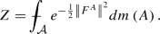
(Formal Yang–Mills Expectations). If $\varPsi :\mathcal {A} \rightarrow \mathbb {C}$ is a restricted gauge invariant function, we define

$$\begin{aligned} \left\langle \varPsi \right\rangle _{YM}:=\frac{1}{Z_{\sigma }}\int _{\mathcal {A} _{\sigma }}\varPsi \left( A\right) e^{-\frac{1}{2}\left\| F^{A}\right\| ^{2}}d\tilde{m}_{\sigma }\left( A\right) , \end{aligned}$$

(B.26)

where $\sigma$ is any follow the leader homotopy, $\tilde{m}_{\sigma }$ is a formal Lebesgue measure on $\mathcal {A}_{\sigma }$, and (formally)

$$\begin{aligned} Z_{\sigma }:=\int _{\mathcal {A}_{\sigma }}e^{-\frac{1}{2}\left\| F^{A}\right\| ^{2}}d\tilde{m}_{\sigma }\left( A\right) . \end{aligned}$$

A few remarks are in order;

• 1. The expression in Eq. (B.26) is formally independent of the choice of Lebesgue measure on $\mathcal {A}_{\sigma }$ since they all differ by a multiplicative constant and any such multiplicative constant will also occur in the normalization constant, $Z_{\sigma }$.

• 2. The expression in Eq. (B.26) is formally independent of the choice of the follow the leader homotopy, $\sigma$, used in the definition since by the first remark we may choose $\tilde{m}_{\sigma }=m_{\sigma }$ in which case

  

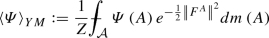  (B.27)

  with

  

Our final goal is to show (formally) that $\left\langle \varPsi \right\rangle _{YM_{2}}$ is invariant under area preserving diffeomorphisms.

1.5 Area preserving diffeomorphisms

Let $\sigma$ be a homotopy contracting $\mathbb {R}^{d}$ to $\left\{ 0\right\}$.

Notation B.44

(Diffeomorphism action on $\mathcal {A}_{\sigma }$). If $\varphi :\mathbb {R}^{d}\rightarrow \mathbb {R}^{d}$ is a diffeomorphism, let ${\hat{\varphi }}_{\sigma }:\mathcal {A}_{\sigma }\rightarrow \mathcal {A}_{\sigma }$ be defined by

$$\begin{aligned} {\hat{\varphi }}_{\sigma }\left( A\right) :=\pi _{\sigma }\left( \varphi ^{*}A\right) =\left( \varphi ^{*}A\right) ^{g_{A}}\text { for all } A\in \mathcal {A}_{\sigma }, \end{aligned}$$

where

$$\begin{aligned} g_{A}\left( p\right) =//_{1}^{A}\left( \varphi \circ \sigma _{p}\right) \text { for all }p\in \mathbb {R}^{d}. \end{aligned}$$

(B.28)

Proposition B.45

(The diffeomorphism action parallel translation). If $\varphi :\mathbb {R}^{d}\rightarrow \mathbb {R}^{d}$ is a diffeomorphism, $A\in \mathcal {A}_{\sigma }$, and $\alpha \in C^{1}\left( \left[ a,b\right] ,\mathbb {R}^{2}\right)$ is a path, then

$$\begin{aligned} //^{{\hat{\varphi }}_{\sigma }\left( A\right) }\left( \alpha \right) =g_{A}\left( \alpha \left( b\right) \right) ^{-1}//^{A}\left( \varphi \circ \alpha \right) g_{A}\left( \alpha \left( a\right) \right) \end{aligned}$$

(B.29)

where $g_{A}$ is as in Eq. (B.28).

Proof

Using Theorem A.1 and Proposition A.3 we have

$$\begin{aligned} //^{{\hat{\varphi }}_{\sigma }\left( A\right) }\left( \alpha \right) =//^{\left[ \varphi ^{*}A\right] ^{g_{A}}}\left( \alpha \right)&=g_{A}\left( \alpha \left( b\right) \right) ^{-1}//^{\left[ \varphi ^{*}A\right] }\left( \alpha \right) g_{A}\left( \alpha \left( a\right) \right) \\&=g_{A}\left( \alpha \left( b\right) \right) ^{-1}//^{A}\left( \varphi \circ \alpha \right) g_{A}\left( \alpha \left( a\right) \right) . \end{aligned}$$

$\square$

For the rest of this appendix we now exclusively assume that $d=2$ and further assume that $\varphi :\mathbb {R}^{2}\rightarrow \mathbb {R}^{2}$ is an area preserving diffeomorphism.

Definition B.46

A diffeomorphism, $\varphi :\mathbb {R}^{2}\rightarrow \mathbb {R}^{2}$ is area preserving provided $\left| \det \varphi ^{\prime }\left( p\right) \right| =1$ for all $p\in \mathbb {R} ^{2}$. We further let $\varepsilon \left( \varphi \right) =\mathrm {sgn}\left( \det \varphi ^{\prime }\right) \in \left\{ \pm 1\right\}$ so that $\varphi$ is orientation preserving if $\varepsilon \left( \varphi \right) =1$ and orientation reversing if $\varepsilon \left( \varphi \right) =-1$. Alternatively stated, a diffeomorphism. $\varphi :\mathbb {R}^{2}\rightarrow \mathbb {R}^{2}$, is area preserving iff $\varphi ^{*}\left( dx\wedge dy\right) =\varepsilon \left( \varphi \right) dx\wedge dy$ where $\varepsilon \left( \varphi \right)$ is either 1 or $-1$. i.e.

Our final goal of this appendix is to “prove” the following Meta-Theorem.

Meta-Theorem B.47

Let $\varphi :\mathbb {R}^{2}\rightarrow \mathbb {R}^{2}$ be an area preserving diffeomorphism and $\varPsi :\mathcal {A}\rightarrow \left[ 0,\infty \right]$ be a function. If either;

• 1. $\varphi \left( 0\right) =0$ and $\varPsi$ is a restricted gauge invariant, or

• 2. $\varPsi$ is invariant under the full gauge group,

then

$$\begin{aligned} \left\langle \varPsi \circ \varphi ^{*}\right\rangle _{YM_{2}}=\left\langle \varPsi \right\rangle _{YM_{2}}. \end{aligned}$$

(B.30)

Proof

(Meta-Proof) This result follows from using either Meta-Theorem B.55 or Meta-Theorem B.56 below along with the observation in the next lemma that $\mathcal {A}\ni A\rightarrow \left\| F^{A}\right\|$ is invariant under $\varphi ^{*}$. $\quad \square$

Lemma B.48

If $\varphi :\mathbb {R}^{2}\rightarrow \mathbb {R}^{2}$ is an area preserving diffeomorphism, then $\left\| F^{\varphi ^{*} A}\right\| =\left\| F^{A}\right\|$ for all $A\in \mathcal {A}$.

Proof

Writing $F^{A}=f^{A}dx_{1}\wedge dx^{2}$ we have

$$\begin{aligned} f^{\varphi ^{*}A}dx_{1}\wedge dx^{2}&=F^{\varphi ^{*}A}=\varphi ^{*}F^{A}=f^{A}\circ \varphi \cdot \varphi ^{*}\left( dx_{1}\wedge dx_{2}\right) \\&=\varepsilon \left( \varphi \right) f^{A}\circ \varphi \cdot dx_{1}\wedge dx_{2} \end{aligned}$$

where $\varepsilon \left( \varphi \right) \in \left\{ \pm 1\right\}$ since $\varphi$ is area preserving and consequently,

$$\begin{aligned} \left\| F^{\varphi ^{*}A}\right\| ^{2}&=\int _{\mathbb {R}^{2} }\left| f^{\varphi ^{*}A}\left( x\right) \right| _{\mathfrak {k} }^{2}dx=\int _{\mathbb {R}^{2}}\left| f^{A}\left( \varphi \left( x\right) \right) \right| _{\mathfrak {k}}^{2}dx\\&=\int _{\mathbb {R}^{2}}\left| f^{A}\left( x\right) \right| _{\mathfrak {k}}^{2}dx=\left\| F^{A}\right\| ^{2}. \end{aligned}$$

$\square$

So it now remains to “prove” Meta-Theorem B.55 and Meta-Theorem B.56 below. In brief these theorems assert; if $\varphi :\mathbb {R}^{2}\rightarrow \mathbb {R}^{2}$ is an area preserving diffeomorphism and $\varPsi :\mathcal {A}\rightarrow \left[ 0,\infty \right]$ is a function, then

(B.31)

provided $\varPsi$ is invariant under the full gauge group (Meta-Theorem B.56) or $\varphi \left( 0\right) =0$ and $\varPsi$ is invariant under the restricted gauge group (Meta-Theorem B.55). Let us note that when $\varphi \left( 0\right) \ne 0$, $\varphi ^{*}g=g\circ \varphi$ will not be in $\mathcal {G}$ for $g\in \mathcal {G}$. Nevertheless, if $\varPsi$ is invariant under the full gauge group, then

$$\begin{aligned} \varPsi \left( \varphi ^{*}A^{g}\right) =\varPsi \left( \left( \varphi ^{*}A\right) ^{\varphi ^{*}g}\right) =\varPsi \left( \varphi ^{*}A\right) \text { }\forall ~g\in \mathcal {G} \end{aligned}$$

and therefore $A\rightarrow \varPsi \left( \varphi ^{*}A\right)$ is still a restricted gauge invariant function on $\mathcal {A}$.

Our “proof” of Eq. (B.31) will boil down to formally verifying the hypothesis of Theorem B.14 in this infinite dimensional setting. It is worth noting that the results to follow hold for any $d\in \mathbb {N}$ with $d\ge 2$ in the special case where $\varphi \left( x\right) =Rx+b$ with R being a rotation on $\mathbb {R}^{d}$ and $b\in \mathbb {R}^{d}$. We now begin “verifying” the hypothesis of Theorem B.14 in this infinite dimensional gauge theory context.

Meta-Lemma B.49

The restricted gauge group, $\mathcal {G}$, is formally unimodular.

Proof

(Meta-Proof) The Lie algebra $\left( \mathrm{Lie}\left( \mathcal {G} \right) \right)$ of $\mathcal {G}$ consists of functions, $\xi :\mathbb {R}^{2}\rightarrow \mathfrak {k}$ with $\xi \left( 0\right) =0$. Let

$$\begin{aligned} \left\langle \xi ,\eta \right\rangle _{\mathrm{Lie}\left( \mathcal {G} \right) }:=\int _{\mathbb {R}^{2}}\left\langle \xi \left( x\right) ,\eta \left( x\right) \right\rangle _{\mathfrak {k}}dx \end{aligned}$$

where $\left\langle \cdot ,\cdot \right\rangle _{\mathfrak {k}}$ is an $\mathrm {Ad}_{K}$—invariant inner product on $\mathfrak {k.}$ If $g\in \mathcal {G}$, then

$$\begin{aligned} \left\| \mathrm {Ad}_{g}\xi \right\| _{\mathrm{Lie}\left( \mathcal {G}\right) }^{2}=\int _{\mathbb {R}^{2}}\left| \mathrm {Ad} _{g\left( x\right) }\xi \left( x\right) \right| _{\mathfrak {k}} ^{2}dx=\int _{\mathbb {R}^{2}}\left| \xi \left( x\right) \right| _{\mathfrak {k}}^{2}dx=\left\| \xi \right\| _{\mathrm{Lie}\left( \mathcal {G}\right) }^{2} \end{aligned}$$

so that $\mathrm {Ad}_{g}$ acts as orthogonal transformation and therefore

$$\begin{aligned} \varDelta _{\mathcal {G}}\left( g\right) =\left| \det \mathrm {Ad}_{g^{-1} }\right| =1. \end{aligned}$$

Alternatively, extended $\left\langle \cdot ,\cdot \right\rangle _{\mathrm{Lie}\left( \mathcal {G}\right) }$ to a left invariant Riemannian metric on $T\mathcal {G}$ and note that the fact that $\mathrm {Ad}_{g}$ is an isometry for $\left\langle \cdot ,\cdot \right\rangle _{\mathrm{Lie}\left( \mathcal {G}\right) }$ implies this Riemannian metric is also right invariant. Thus the Riemannian volume measure associated to this Riemannian metric is both right and left invariant and so this measure is both a left and a right invariant Haar measure. $\quad \square$

Lemma B.50

If $\varphi :\mathbb {R}^{2}\rightarrow \mathbb {R}^{2}$ is an area preserving diffeomorphism such that $\varphi \left( 0\right) =0$, then $\gamma :\mathcal {G}\rightarrow \mathcal {G}$ defined by $\gamma \left( g\right) =\varphi ^{*}g$ is a group isomorphism⁴ such that

$$\begin{aligned} \varphi ^{*}\left( A\cdot g\right) =\varphi ^{*}A\cdot \gamma \left( g\right) \text { }\forall ~A\in \mathcal {A}\text { and }g\in \mathcal {G}. \end{aligned}$$

Proof

This result is a consequence of the following elementary computation;

$$\begin{aligned} \varphi ^{*}\left( A\cdot g\right)&=\varphi ^{*}\left( A^{g}\right) =\varphi ^{*}\left[ \mathrm {Ad}_{g^{-1}}A+g^{-1}dg\right] \\&=\left[ \mathrm {Ad}_{\left( g\circ \varphi \right) ^{-1}}\varphi ^{*}A+\left( g\circ \varphi \right) ^{-1}d\left( g\circ \varphi \right) \right] \\&=\varphi ^{*}A\cdot \varphi ^{*}g. \end{aligned}$$

$\square$

Meta-Lemma B.51

Let $\varphi$ and $\gamma$ be as in Lemma B.50. Then $\gamma$ preserves Haar measure on $\mathcal {G}$ and hence $c_{\gamma }=1$ where $c_{\gamma }$ was defined in Eq. (B.11).

Proof

(Meta-Proof) For $g\in \mathcal {G}$ and $\xi \in \mathrm{Lie}\left( \mathcal {G}\right)$ let $\tilde{\xi }\left( g\right) =L_{g*}\xi$ be the left invariant extension of $\xi$. Then

$$\begin{aligned} \gamma _{*}\tilde{\xi }\left( g\right) =\frac{d}{dt}|_{0}\gamma \left( ge^{t\xi }\right) =\frac{d}{dt}|_{0}\gamma \left( g\right) \gamma \left( e^{t\xi }\right) =L_{\gamma \left( g\right) *}\gamma _{*}\xi =L_{\gamma \left( g\right) *}\left[ \xi \circ \varphi \right] . \end{aligned}$$

By construction of the Riemannian metric on $\mathcal {G}$, $L_{\gamma \left( g\right) *}$ is an isometry and therefore (using $\varphi$ is area preserving) we find

$$\begin{aligned} \left\langle \gamma _{*}\tilde{\xi }\left( g\right) ,\gamma _{*} \tilde{\xi }\left( g\right) \right\rangle _{T_{\gamma \left( g\right) }\mathcal {G}}&=\left\langle \xi \circ \varphi ,\xi \circ \varphi \right\rangle _{\mathrm{Lie}\left( \mathcal {G}\right) }\\&=\int _{\mathbb {R}^{2}}\left| \xi \left( \varphi \left( x\right) \right) \right| _{\mathfrak {k}}^{2}dx=\int _{\mathbb {R}^{2}}\left| \xi \left( x\right) \right| _{\mathfrak {k}}^{2}dx=\left\langle \tilde{\xi }\left( g\right) ,\tilde{\xi }\left( g\right) \right\rangle _{T_{g}\mathcal {G}}. \end{aligned}$$

This shows $\gamma :\mathcal {G}\rightarrow \mathcal {G}$ is a Riemannian isometry and hence preserves the (fictitious) Riemannian volume measure on $\mathcal {G}$. As this volume measure is precisely Haar measure the “proof” is complete. $\quad \square$

The last item we need to verify is that $\varphi ^{*}:\mathcal {A} \rightarrow \mathcal {A}$ preserves Lebesgue measure when $\varphi$ is an area preserving diffeomorphisms on $\mathbb {R}^{2}$. To do this we will make use of the following meta-lemma.

Meta-Lemma B.52

Let V be a finite dimensional inner product space and $U:\mathbb {R}^{2}\rightarrow \mathrm{End}\left( V\right)$ be a function such that $\det U\left( x\right) =1$ for all $x\in \mathbb {R}^{2}$. If $M_{U}:L^{2}\left( \mathbb {R}^{2};V\right) \rightarrow L^{2}\left( \mathbb {R}^{2};V\right)$ is the operation of multiplication by U, then $\,\det M_{U}=1$ or more usefully stated; the map, $f\rightarrow Uf$, leaves Lebesgue measure invariant.

Proof

(Meta-Proof). Here we suppose that $U\left( x\right) =U_{1}\left( x\right)$ where $\left\{ U_{t}\left( x\right) \right\} _{t\in \left[ 0,1\right] }$ is a one parameter ($C^{1}$ in t) family of functions in $SL\left( V\right)$ with $U_{0}\left( x\right) =I$ for all x. Further let $\alpha _{t}\left( x\right) :=U_{t}\left( x\right) ^{-1}\dot{U}_{t}\left( x\right)$ so that $\dot{U}_{t}\left( x\right) =\alpha _{t}\left( x\right) U_{t}\left( x\right)$ with $U_{0}\left( x\right) =I$ and ${\text {tr}}\left( \alpha _{t}\left( x\right) \right) =0$. We then formally should have,

$$\begin{aligned} \frac{d}{dt}\det \left[ M_{U_{t}}\right] =\det \left[ M_{U_{t}}\right] {\text {Tr}}\left[ M_{U_{t}^{-1}}M_{\dot{U}_{t}}\right] =\det \left[ M_{U_{t}}\right] {\text {Tr}}\left[ M_{\alpha _{t}}\right] \end{aligned}$$

(B.32)

where ${\text {Tr}}$ is the infinite dimensional trace on $L^{2}\left( \mathbb {R}^{d},V\right)$. To evaluate the trace, let $\left\{ u_{m}\right\} _{m=1}^{\infty }$ be an orthonormal basis for $L^{2}\left( \mathbb {R}^{d},\mathbb {R}\right)$ and $\left\{ e_{i}\right\} _{i=1}^{\dim V}$ be an orthonormal basis for V relative to some fixed inner product on V. Then

$$ \begin{aligned} \left\{ u_{m}\cdot e_{i}:m\in \mathbb {N} \, \& \, 1\le i\le \dim V\right\} \end{aligned}$$

is an orthonormal basis for $L^{2}\left( \mathbb {R} ^{d},V\right)$ and hence it is reasonable to compute ${\text {Tr}} \left( M_{\alpha _{t}}\right)$ as,

$$\begin{aligned} {\text {Tr}}\left( M_{\alpha _{t}}\right)&=\sum _{m=1}^{\infty } \sum _{i=1}^{d}\left\langle M_{\alpha _{t}}u_{m}\cdot e_{i},u_{m}\cdot e_{i}\right\rangle _{L^{2}\left( \mathbb {R}^{d},V\right) }\\&=\sum _{m=1}^{\infty }\sum _{i=1}^{d}\int _{\mathbb {R}^{2}}\left\langle \alpha _{t}\left( x\right) e_{i},e_{i}\right\rangle u_{m}^{2}\left( x\right) dx\\&=\sum _{m=1}^{\infty }\int _{\mathbb {R}^{2}}{\text {tr}}\left[ \alpha _{t}\left( x\right) \right] u_{m}^{2}\left( x\right) dx=\sum _{m=1}^{\infty }\int _{\mathbb {R}^{2}}0\cdot u_{m}^{2}\left( x\right) dx=0. \end{aligned}$$

Thus we have shown $\det \left[ M_{U_{t}}\right]$ is constant in t and so

$$\begin{aligned} \det M_{U}=\det \left[ M_{U_{1}}\right] =\det \left[ M_{U_{0}}\right] =\det I_{L^{2}\left( \mathbb {R}^{2};V\right) }=1. \end{aligned}$$

$\square$

Remark B.53

The computation of the trace of $M_{\alpha _{t}}$ above is certainly not rigorous as $M_{\alpha _{t}}$ is not a trace class operator.

Meta-Proposition B.54

If $\varphi :\mathbb {R}^{2}\rightarrow \mathbb {R}^{2}$ is an area preserving diffeomorphism, then the induced map, $\mathcal {A\ni }A\rightarrow \varphi ^{*}A\in \mathcal {A}$ formally preserves Lebesgue measure on $\mathcal {A}$.

Proof

(Meta-Proof). If $A=A_{1}dx_{1}+A_{2}dx_{2}$, then

$$\begin{aligned} \varphi ^{*}A&=A_{1}\circ \varphi d\left[ x_{1}\circ \varphi \right] +A_{2}\circ \varphi d\left[ x_{2}\circ \varphi \right] \\&=A_{1}\circ \varphi \left[ \partial _{1}\varphi _{1}dx_{1}+\partial _{2} \varphi _{1}dx_{2}\right] +A_{2}\circ \varphi \left[ \partial _{1}\varphi _{2}dx_{1}+\partial _{2}\varphi _{2}dx_{2}\right] \\&=\left( \left[ A_{1}\circ \varphi \right] \partial _{1}\varphi _{1}+\left[ A_{2}\circ \varphi \right] \partial _{1}\varphi _{2}\right) dx_{1}+\left( \left[ A_{1}\circ \varphi \right] \partial _{2}\varphi _{1}+\left[ A_{2} \circ \varphi \right] \partial _{2}\varphi _{2}\right) dx_{2}. \end{aligned}$$

Thus identifying A with $\left[ \begin{array} [c]{cc} A_{1}&A_{2} \end{array} \right] ^{{\text {tr}}}$, the transformation $\mathcal {A\ni } A\rightarrow \varphi ^{*}A\in \mathcal {A}$ is the composition of the linear transformation

$$\begin{aligned} \left[ \begin{array} [c]{c} A_{1}\\ A_{2} \end{array} \right] \rightarrow \left[ \begin{array} [c]{c} A_{1}\\ A_{2} \end{array} \right] \circ \varphi \end{aligned}$$

(B.33)

followed by applying the linear transformation, $M_{U}$, where

$$\begin{aligned} U\left( x,y\right) :=\left[ \begin{array} [c]{cc} \left( \partial _{1}\varphi _{1}\right) \left( x,y\right) &{} \left( \partial _{1}\varphi _{2}\right) \left( \left( x,y\right) \right) \\ \left( \partial _{2}\varphi _{1}\right) \left( x,y\right) &{} \left( \partial _{2}\varphi _{2}\right) \left( \left( x,y\right) \right) \end{array} \right] . \end{aligned}$$

The assumption that $\varphi$ is area preserving is equivalent to $\det U\left( x,y\right) =1$ and hence by Meta-Lemma B.52, ${\text {Det}}\left[ M_{U}\right] =1$. The assumption that $\varphi$ is area preserving also implies that transformation in Eq. (B.33) is an isometry on $L^{2}\left( \mathbb {R}^{2};\mathfrak {k}^{2}\right)$ and so again (formally) preserves Lebesgue measure. As $A\rightarrow \varphi ^{*}A$ is a composition of two Lebesgue measure preserving maps it also (formally) preserves Lebesgue measure on $\mathcal {A}$. $\quad \square$

Meta-Theorem B.55

Let $d=2$. If $\varphi$ is an area preserving diffeomorphism such that $\varphi \left( 0\right) =0$ and $\varPsi$ is a restricted gauge invariant function, then formally Eq. (B.31) holds.

Proof

This result heuristically follows from Theorem B.14 whose hypothesis have been heuristically verified in Meta-Lemmas B.49 and B.51 and Meta-Proposition B.54. $\quad \square$

Meta-Theorem B.56

Let $d=2$. If $\varphi$ is an area preserving diffeomorphism and $\varPsi$ is invariant under the full gauge group, then (formally) Eq. (B.31) still holds.

Proof

If $\varphi \left( 0\right) =0$ the result follows from Meta-Theorem B.55. When $\varphi \left( 0\right) \ne 0$ we let $\eta \left( \cdot \right) :=\varphi \left( \cdot \right) -\varphi \left( 0\right)$. Then $\varphi =\eta +\varphi \left( 0\right)$ which shows $\varphi$ is the composition of an area preserving diffeomorphism $\left( \eta \right)$ fixing $0\in \mathbb {R}^{2}$ followed by translation by $\varphi \left( 0\right)$. Thus to finish the proof it suffices to consider the special case where $\varphi \left( x\right) =x+b$ for some vector $b\in \mathbb {R}^{2}$. We can further reduce the problem to the case where $b\in \mathbb {R}e_{1}$ where $e_{1}=\left( 0,1\right)$. To verify this, let R be the $2\times 2$ rotation matrix such that $R^{-1}b=v\in \mathbb {R}e_{1}$ and then write $\varphi$ as $\varphi \left( x\right) =R\left[ R^{-1}x+v\right]$. This shows that $\varphi$ is a composition of two area preserving diffeomorphism, R and $R^{-1}$, which fix $0\in \mathbb {R}^{2}$ along with a translation by $v\in \mathbb {R}e_{1}$.

Owing to the above reductions we now assume that $\varphi \left( x\right) =x+\lambda e_{1}$ for some $\lambda \in \mathbb {R}$. Let $\sigma$ be the complete axial homotopy in Example B.20 in which case $A\in \mathcal {A}_{\sigma }$ iff $A=A_{1}dx_{1}\in \mathcal {A}_{\sigma }$ with $A_{1}\left( x_{1},0\right) =0$ for all $x_{1}\in \mathbb {R}$. Since, for $A\in \mathcal {A}_{\sigma }$

$$\begin{aligned} \varphi ^{*}\left( A_{1}dx_{1}\right) =A_{1}\circ \varphi dx_{1} =A_{1}\left( \cdot +\lambda ,\cdot \right) dx_{1} \end{aligned}$$

it follows that $\varphi ^{*}$ preserves $\mathcal {A}_{\sigma }$. Moreover, as $\varphi ^{*}$ acts orthogonally on $\mathcal {A}_{\sigma }$ equipped with the $L^{2}\left( \mathbb {R}^{2},\mathfrak {k}\right)$-inner product it is reasonable to (formally) assert that $\varphi ^{*}$ leaves “Lebesgue measure” on $\mathcal {A}_{\sigma }$ invariant. As $m_{\sigma }$ is formally a Lebesgue measure on $\mathcal {A}_{\sigma }$ by Meta-Proposition B.40, we conclude that

$\square$

References

Cébron, G., Dahlqvist, A., Gabriel, F.: The generalized master fields. J. Geom. Phys. 119, 34–53 (2017)
Charalambous, N., Gross, L.: The Yang–Mills heat semigroup on three-manifolds with boundary. Commun. Math. Phys. 317(3), 727–785 (2013)
Charalambous, N., Gross, L.: Neumann domination for the Yang–Mills heat equation. J. Math. Phys. 56(7), 073505-1-073505-21 (2015)
Charalambous, N., Gross, L.: Initial behavior of solutions to the Yang–Mills heat equation. J. Math. Anal. Appl. 451(2), 873–905 (2017)
Chatterjee, S.: Rigorous solution of strongly coupled SO(N) lattice gauge theory in the large N limit, ArXiv e-prints (2015)
Chatterjee, S., Jafarov, J.: The 1/N expansion for SO(N) lattice gauge theory at strong coupling. ArXiv e-prints (2016)
Chatterjee, S.: The leading term of the Yang–Mills free energy. J. Funct. Anal. 271(10), 2944–3005 (2016)
Dahlqvist, A., Norris, J.: Yang–Mills measure and the master field on the sphere. ArXiv e-prints (2017)
Dahlqvist, A.: Free energies and fluctuations for the unitary Brownian motion. Commun. Math. Phys. 348(2), 395–444 (2016)
Dellacherie, C.: Capacités et processus stochastiques. Ergebnisse der Mathematik und ihrer Grenzgebiete, Band 67. Springer-Verlag, Berlin (1972)
D’Hoker, E.: Quantum field theory: part I. Department of Physics and Astronomy, UCLA, Lecture Notes, Oct 2004. http://www.pa.ucla.edu/content/eric-dhoker-graduate-lecture-notes. Accessed 7 April 2017
Driver, B.K.: Classifications of bundle connection pairs by parallel translation and lassos. J. Funct. Anal. 83(1), 185–231 (1989)
Driver, B.K.: \(\text{ YM }_2\): continuum expectations, lattice convergence, and lassos. Commun. Math. Phys. 123(4), 575–616 (1989)
Driver, B.K., Gabriel, F., Hall, B.C., Kemp, T.: The Makeenko–Migdal equation for Yang–Mills theory on compact surfaces. Commun. Math. Phys. 352(3), 967–978 (2017)
Driver, B.K., Hall, B.C., Kemp, T.: Three proofs of the Makeenko–Migdal equation for Yang–Mills theory on the plane. Commun. Math. Phys. 351(2), 741–774 (2017)
Gopakumar, R., Gross, D.J.: Mastering the master field. Nucl. Phys. B 451(1–2), 379–415 (1995)
Gross, L.: The Yang–Mills heat equation with finite action. ArXiv e-prints (2016)
Gross, L.: A Poincaré lemma for connection forms. J. Funct. Anal. 63(1), 1–46 (1985)
Gross, L., King, C., Sengupta, A.: Two-dimensional Yang–Mills theory via stochastic differential equations. Ann. Phys. 194(1), 65–112 (1989)
Hall, B.C.: The large-N limit for two-dimensional Yang–Mills theory. ArXiv e-prints (2017)
Janson, S.: Gaussian Hilbert Spaces. Cambridge Tracts in Mathematics, vol. 129. Cambridge University Press, Cambridge (1997)
Kazakov, V.A., Kostov, I.K.: Nonlinear strings in two-dimensional \(U(\infty )\) gauge theory. Nucl. Phys. B 176(1), 199–215 (1980)
Kazakov, V.A.: Wilson loop average for an arbitrary contour in two-dimensional U(N) gauge theory. Nucl. Phys. B 179(2), 283–292 (1981)
Lévy, T.: The master field on the plane. Astérisque, no. 388, ix+201 (2017)
Makeenko, Y.M., Migdal, A.A.: Exact equation for the loop average in multicolor QCD. Phys. Lett. B 88(1), 135–137 (1979)
Nguyen, T.: Quantum Yang–Mills theory in two dimensions: exact versus perturbative. ArXiv e-prints (2015)
Nguyen, T.: Stochastic Feynman rules for Yang–Mills theory on the plane. ArXiv e-prints (2016)
Nguyen, T.: Wilson loop area law for 2D Yang–Mills in generalized axial gauge. ArXiv e-prints (2016)
Nguyen, T.: The perturbative approach to path integrals: a succinct mathematical treatment. J. Math. Phys. 57(9), 092301-1-092301-27 (2016). (see Section III for gauge fixing from a differential form point of view)
Sengupta, A.: Quantum Yang–Mills theory on compact surfaces. In: Cardoso, A.I., de Faria, M., Potthoff, J., Sénéor, R., Streit, L. (eds.) Stochastic Analysis and Applications in Physics. NATO ASI Series (Series C: Mathematical and Physical Sciences), vol. 449, pp. 389–403. Kluwer Academic Publishers, Dordrecht (1994)
Sengupta, A.: Gauge Theory on Compact Surfaces. Memoirs of The American Mathematical Society, vol. 126. American Mathematical Society, Providence (1997)
Sengupta, A.: Yang–Mills on surfaces with boundary: quantum theory and symplectic limit. Commun. Math. Phys. 183(3), 661–705 (1997)
Sengupta, A.N.: Traces in two-dimensional QCD: the large-N limit. In: Albeverio, S., Marcolli, M., Paycha, S., Plazas, J. (eds.) Traces in Number Theory, Geometry and Quantum Fields. Aspects Mathematics, E38, pp. 193–212. Friedr. Vieweg, Wiesbaden (2008)
Weinberg, S.: The Quantum Theory of Fields, vol. II. Cambridge University Press, Cambridge (2005). (modern applications)
Acknowledgements
It is a pleasure to acknowledge useful discussions with Brian Hall, Len Gross, and Todd Kemp pertaining to this work. The author is also very grateful to the anonymous referees for their corrections and useful comments on this manuscript.
Author information
Authors and Affiliations
Corresponding author
Additional information
Communicated by M. Hairer
Publisher's Note
Springer Nature remains neutral with regard to jurisdictional claims in published maps and institutional affiliations.