
Abstract
Since their introduction in 1967, Lawson methods have achieved constant interest in the time discretization of evolution equations. The methods were originally devised for the numerical solution of stiff differential equations. Meanwhile, they constitute a well-established class of exponential integrators, which has turned out to be competitive for solving space discretizations of certain types of partial differential equations. The popularity of Lawson methods is in some contrast to the fact that they may have a bad convergence behaviour, since they do not satisfy any of the stiff order conditions. The aim of this paper is to explain this discrepancy. It is shown that non-stiff order conditions together with appropriate regularity assumptions imply high-order convergence of Lawson methods. Note, however, that the term regularity here includes the behaviour of the solution at the boundary. For instance, Lawson methods will behave well in the case of periodic boundary conditions, but they will show a dramatic order reduction for, e.g., Dirichlet boundary conditions. The precise regularity assumptions required for high-order convergence are worked out in this paper and related to the corresponding assumptions for splitting schemes. In contrast to previous work, the analysis is based on expansions of the exact and the numerical solution along the flow of the homogeneous problem. Numerical examples for the Schrödinger equation are included.
1 Introduction
Exponential integrators are a well-established class of methods for the numerical solution of semilinear stiff differential equations. If the problem stems from a spatial discretization of an evolutionary partial differential equation (PDE), the very form of the domain of the spatial differential operator enters the convergence analysis. The stiff order conditions, which guarantee a certain order of convergence independently of the considered problem, however, must be independent of the domain of this operator (which, in general, involves certain boundary conditions). This is the main reason why stiff order conditions for exponential integrators are quite involved (see [9, 16]).
For particular problems, however, less conditions are often required for obtaining a certain order of convergence.Footnote 1 It was already observed in [10] that periodic boundary conditions do not lead to any order reduction in exponential integrators of collocation type in contrast to homogeneous Dirichlet boundary conditions, which restrict the order of convergence considerably (close to the stage order, depending on the precise situation). Full-order convergence for periodic boundary conditions was also noticed for exponential time-differencing methods in [13].
A similar behaviour can be observed for Lawson methods which are obtained by a linear variable transformation from (explicit) Runge–Kutta methods (see [15] and Sect. 2 below). These methods are very attractive, since they can be easily constructed from any known Runge–Kutta method. Unfortunately, Lawson methods exhibit a strong order reduction, in general. For particular problems, however, they show full order of convergence, see [2,3,4,5, 18]. Lawson methods have also been used successfully in [1] for applications in optical fibres. By construction, Lawson methods do satisfy the order conditions for non-stiff problems. Such conditions will be called non-stiff or classical order conditions henceforth. However, Lawson methods do not satisfy any of the stiff order conditions, as detailed in [9, 11, 16]. This fact can result in a dramatic order reduction, even down to order one for parabolic problems with homogeneous Dirichlet boundary conditions. On the other hand, in [4], full order of convergence was shown for an implicit Lawson method based on Gauss points for a nonlinear Schrödinger equation with periodic boundary conditions.
So far, the derivation of (stiff) order conditions for exponential integrators was based on standard expansions of the exact and the numerical solution. There, the main assumption on the problem is that the exact solution and its composition with the nonlinearity are both sufficiently smooth in time (see [9, 16]). Any additional regularity in space is not of immediate benefit in this analysis. This is in contrast to splitting methods, where spatial regularity usually shows up in form of commutator bounds (see, e.g., [12]).
In this paper, we study the convergence behaviour of Lawson methods for semilinear problems. One of the main contributions of this paper is a different expansion of the solution. It is still based on the variation-of-constants formula but the nonlinearity is expanded along the flow of the homogeneous problem. This expansion can be derived in a systematic way using trees as in [7, 16]. The expansion of the exact solution is carried out in terms of elementary integrals, that of the numerical solution in terms of elementary quadrature rules. We show that classical, non-stiff order conditions together with (problem-dependent) assumptions on the exact solution give full order of convergence. This involves regularity of the solution in space and time. Our main result for Lawson methods is stated in Theorems 4.7 and 4.8. We prove that a Lawson method converges with order p, if the order of the underlying Runge–Kutta method is at least p and the solution satisfies appropriate regularity assumptions. These conditions are studied in detail for methods of orders one and two, respectively, and they are related to the corresponding conditions that arise in the analysis of splitting methods. In particular, this is worked out for the nonlinear Schrödinger equation. Our error analysis also reveals a different behaviour between the first-order Lawson method and the exponential Euler method, which is visible in numerical experiments.
The outline of the paper is as follows. In Sect. 2, we recall the construction of Lawson methods. The expansion of the numerical and the exact solution in terms of elementary integrals is given in Sect. 3. There, we also introduce the analytic (finite dimensional) framework which typically occurs when discretizing a semilinear parabolic or hyperbolic PDE in space. Order conditions and convergence results are given in Sect. 4. The resulting regularity assumptions are discussed in Sect. 5. These assumptions are related to the corresponding conditions for splitting methods. Numerical examples that illustrate the required regularity assumptions and the proven convergence behaviour are also presented.
2 Lawson methods
Consider a semilinear system of stiff differential equations
where the stiffness stems from the linear part of the equation, i.e., from A, which is either an unbounded linear operator or its spatial discretization, i.e., a matrix. The precise assumptions on A and g will be given in Sect. 3. For the sake of presentation, we choose \(t_0=0\) as initial time (otherwise we can apply a simple time shift). For the numerical solution of (1), Lawson [15] considered the following local change of variables:
Note that when applied to evolution equations, this transformation has to be done in a formal way, since \(\hbox {e}^{t A}\) might not be a meaningful object in our general framework.
Inserting the new variables into (1) gives the transformed differential equation
For the solution of this problem, an \(s\)-stage explicit Runge–Kutta method with coefficients \(b_i,c_i, a_{ij}\) satisfying the simplifying assumptions \(c_1=0\) and
is considered. Transforming the Runge–Kutta discretization of (2) back to the original variables yields the corresponding Lawson method for (1)
Here, \(u_n\) is the numerical approximation to the exact solution u(t) at time \(t=t_n=n h\), and \(h\) is the step size. Note that this method makes explicit use of the action of the matrix exponential function. Depending on the properties of A, the nodes \(c_1,\ldots ,c_s\) have to fulfill additional assumptions, see Assumption 3.1 in the next section. Because of these actions of the matrix exponential, Lawson methods form a particular class of exponential integrators. For a review on such integrators, we refer to [11].
For a non-stiff ordinary differential equation (1), it is obvious that the order of the Runge–Kutta method applied to (2) coincides with that of the corresponding Lawson method applied to (1). It is the aim of this paper to show that this is also true in the stiff situation, if appropriate regularity assumptions hold (we will explain the meaning of regularity in the context of discretized PDEs in Sect. 5).
3 Expansion of the exact and the numerical solution
By adding \(t'=1\) to (1), the differential equation is transformed to autonomous form. It is well known that Runge–Kutta methods of order at least one satisfying (3) are invariant under this transformation. Therefore, we restrict ourselves henceforth to the autonomous problem
Let X be a Banach space with norm \(\left\| \,\cdot \, \right\| \). Our main assumptions on A and g are as follows.
Assumption 3.1
Let A belong to a family \({\mathcal {F}}\) of linear operators on X such that \(-A\) generates a group \(\hbox {e}^{-tA}\) satisfying
with a moderate constant \(C_{\mathcal {F}}\), uniformly for all \(t \in {\mathbb {R}}\) and all operators \(A\in {\mathcal {F}}\). It is sufficient to require that \(-A\) generates a bounded semigroup (i.e., (6) for \(t\ge 0\)), if the nodes \(c_i\) of the considered explicit Runge–Kutta method are ordered as \(0=c_1\le c_2\le \cdots \le c_s\le 1\).
The set of infinitesimal generators of non-expansive (semi)groups in X is a possible choice for the family \({\mathcal {F}}\). In addition, the above assumption is typically satisfied in situations where (5) stems from a spatial discretization of a semilinear parabolic or hyperbolic partial differential equation. The important fact here is that the constant \(C_{\mathcal {F}}\) is independent of the spatial mesh width for finite difference and finite element methods, and independent of the number of ansatz functions in spectral methods. As our error bounds derived below do not depend on A itself but only on the constant \(C_{\mathcal {F}}\), they also apply to spatially discretized systems.
Assumption 3.2
For a given integer \(p\ge 0\), the nonlinearity g is p times differentiable with bounded derivatives in a neighborhood of the solution of (5).
Note that Assumptions 3.1 and 3.2 will be required in the rest of the paper without further mentioning it everywhere.
We recall that the solution of (5) can be represented in terms of the variation-of-constants formula
Applying this formula recursively and expanding the nonlinearity along the flow of the homogeneous problem yields the following expansion of the exact solution
where we have used the shorthand notation
Note that here and throughout the whole section, the constant in the Landau symbol \({{\mathcal {O}}}\) only depends on \(C_{\mathcal {F}}\) and the derivatives of g, but not explicitly on A itself, i.e., not on the stiffness. Also note that this expansion differs considerably from the previous work (see, e.g., [9, 16]) where the nonlinearity g(u(t)) was expanded with respect to t.
Next we perform a similar expansion of the numerical solution (4), which yields (again in the autonomous case)
As we have used the variation-of-constants formula and its discrete counterpart, respectively, the expansions of the exact and the numerical solution reflect the well-known tree structure of (explicit) Runge–Kutta methods.
In the following we use the classic trees which are well-established for studying the classical order conditions for Runge–Kutta methods; see [7, Section II.2], [6, Section III.1] and references given there.
Let \({{\mathcal {L}} {{\mathcal {T}}}}\) denote the set of rooted labelled trees; see Def. II.2.2 in [7]. Their nodes are numbered in such a way that the number of a children’s node is larger than that of the corresponding mother’s node. The set \({{\mathcal {T}}}\) of unlabelled rooted trees is defined (as in [7, Def. II.2.4]) as equivalence classes of labelled trees under admissible renumbering.
For \({{\mathcal {S}}}= {{\mathcal {T}}}\) or \({{\mathcal {S}}}= {{\mathcal {L}} {{\mathcal {T}}}}\), respectively, and \(\tau _1,\ldots ,\tau _k \in {{\mathcal {S}}}\) we denote by \(\tau = [\tau _1,\ldots ,\tau _k]\in {{\mathcal {S}}}\) (a k tuple without ordering) the tree that consists of a new root which is connected to the branches \(\tau _1,\ldots ,\tau _k\). Furthermore, by \(\varrho (\tau )\) we denote the order of the tree \(\tau \in {{\mathcal {S}}}\). It is defined as the number of nodes of \(\tau \). Trees of order less or equal than p are denoted by
For \(\tau \in {{\mathcal {T}}}\) the elementary differential \(D(\tau )\) of a smooth function g is defined recursively in the following way. For  we have
  , and for \(\tau = [\tau _1,\ldots ,\tau _k]\) we have
Motivated by the expansion (7) of the exact solution we define elementary integrals.
Definition 3.3
For \(\tau \in {{\mathcal {L}} {{\mathcal {T}}}}\) and \(0 \le \zeta \le 1\) we define the elementary integral\(G_\zeta (\tau )\), its integrand\(\varPsi _\zeta (\tau )\), and the multivariate integration operator\(I_{\zeta }(\tau )\) with its domain of integration \({\mathcal {D}}_\zeta (\tau )\), recursively in the following way.
-
(a)
For
 and a univariate function f, we set
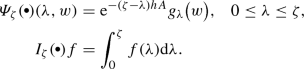
-
(b)
For \(\tau = [\tau _1,\ldots ,\tau _k]\in {{\mathcal {L}} {{\mathcal {T}}}}\) and a multivariate function f in \(\varrho =\varrho (\tau )\) variables, we set (for \(0\le \lambda \le \zeta \))
$$\begin{aligned} \varPsi _\zeta (\tau )(\lambda ,\lambda _2,\ldots ,\lambda _{\varrho },w)&= \hbox {e}^{-(\zeta -\lambda ) hA} g_\lambda ^{(k)}\bigl (w \bigr ) \bigl (\varPsi _\lambda (\tau _1)(\cdot _1,w),\ldots ,\varPsi _\lambda (\tau _k)(\cdot _k,w)\bigr ),\\ I_{\zeta }(\tau )f&= \int _0^\zeta I_{\lambda }(\tau _1)\cdots I_{\lambda }(\tau _k) f(\lambda ,\cdot ,\ldots ,\cdot ) \hbox {d}\lambda . \end{aligned}$$
 and a univariate function f, we set
Here, \(\cdot _j\) refers to the \(\varrho (\tau _j)\) variables corresponding to the jth subtree \(\tau _j\), i.e., all the indices numbering the nodes in \(\tau _j\), sorted in increasing order. The integral operator \(I_{\lambda }(\tau _j)\) acts on the variables corresponding to \(\tau _j\).
Finally, we define for all \(\tau \in {{\mathcal {L}} {{\mathcal {T}}}}\) the elementary integrals as
and set \(\varPsi (\tau ) = \varPsi _1(\tau )\), \({\mathcal {D}}(\tau )=\mathcal D_1(\tau )\), \(I_{}(\tau )=I_{1}(\tau )\), and \(G(\tau ) = G_1(\tau )\).
Example 3.4
With the definition of the integrands we obtain

and

If f is a function of four variables, the recursive definition of the integral yields

with

and

respectively. Here, the integration domain is given by

Note that  integrates with respect to the second and third variable of f whereas
  integrates with respect to the second and forth one. However, the definitions are invariant under permutation of the trees \(\tau _1,\ldots ,\tau _k\).
Although the numbering of the multivariate integration operator and integrands depends on the numbering of the labelled trees, the definition of the elementary integrals is independent of it.
Lemma 3.5
The elementary integral \(G_\zeta (\tau )\) is invariant under renumbering of \(\tau \in {{\mathcal {L}} {{\mathcal {T}}}}\). Thus, it is well defined for unlabelled rooted trees \(\tau \in {{\mathcal {T}}}\) by using one representative of the corresponding equivalence class. \(\square \)
It is straightforward to verify that the elementary integrals satisfy the recurrence relation

for \(\tau =[\tau _1,\ldots ,\tau _k]\in {{\mathcal {T}}}\).
Our assumptions on g and A ensure that the integrand \(\varPsi _\zeta (\tau )(\cdot ,w)\) is bounded if \(\tau \in {{\mathcal {L}} {{\mathcal {T}}}}_{p+1}\) for w in a neighborhood of the exact solution of (5) and \(h\) sufficiently small.
Remark 3.6
In the nonstiff situation, where \(A\equiv 0\), all evaluations of g or its derivatives are at the fixed value w. Thus \(G_\zeta (\tau )(w)\) reduces to a multivariate integral over the constant integrand \(\varPsi _\zeta (\tau )(\cdot ,w) \equiv D(\tau )(w)\).
The following theorem shows how the expansion (7) can be expressed as a (truncated) B-series. Here we use the notation from [6, Section III.1].
Theorem 3.7
The exact solution of (1) satisfies
where we define the B-series for \(w \in X\) and \(\zeta \in [0,1]\) as
with the symmetry coefficients  and
and
The integers \(\mu _1,\mu _2, \ldots \) specify the number of equal trees among \(\tau _1, \ldots , \tau _k\).
Proof
The proof is done by induction. For \(p=0\), the claim follows from the variation-of-constants formula and \(B_{0}(u_0)(\zeta ) = 0\), since
The induction step follows the lines of the proof of [6, Lemma III.1.9] with the following modifications: we use the variation-of-constants formula and truncate the series in such a way that only the first p derivatives of g enter the expansion. We omit the details. \(\square \)
Now we proceed analogously for the numerical solution starting with the definition of elementary quadrature rules.
Definition 3.8
For \(\tau \in {{\mathcal {L}} {{\mathcal {T}}}}\) we define the multivariate quadrature operators\(\widehat{I}(\tau )\) and \( \widehat{I}_{i}(\tau )\), \(i=1,\ldots ,s\), recursively in the following way.
-
(a)
For
 and a univariate function f, we set
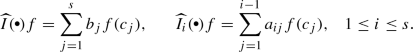
-
(b)
For \(\tau = [\tau _1,\ldots ,\tau _k]\in {{\mathcal {L}} {{\mathcal {T}}}}\) and a multivariate function f in \(\rho (\tau )\) variables, we set
$$\begin{aligned} \widehat{I}(\tau )f&= \sum _{j=1}^s b_j \widehat{I}_{j}(\tau _1)\cdots \widehat{I}_{j}(\tau _k) f(c_j,\cdot ,\ldots ,\cdot ),\\ \widehat{I}_{i}(\tau )f&= \sum _{j=1}^{i-1} a_{ij} \widehat{I}_{j}(\tau _1)\cdots \widehat{I}_{j}(\tau _k) f(c_j,\cdot ,\ldots ,\cdot ),\quad 1\le i \le s. \end{aligned}$$As in Defintion 3.3, the quadrature operator \(\widehat{I}_{j}(\tau _\ell )\) acts on the variables corresponding to labels in \(\tau _\ell \).
 and a univariate function f, we set
Finally, we define the elementary quadrature rules in the following way
As for the elementary integrals, also the elementary quadrature rules do not depend on the numbering of the nodes in a tree.
Lemma 3.9
The elementary quadrature rules \(\widehat{G}(\tau )\) and \(\widehat{G}_i(\tau )\) are invariant under renumbering of \(\tau \in {{\mathcal {L}} {{\mathcal {T}}}}\). Thus, they are well defined for unlabelled rooted trees \(\tau \in {{\mathcal {T}}}\) by using one representative of the corresponding equivalence class. \(\square \)
It is easy to see from the recursive definitions that the elementary quadrature rules satisfy

and
for \(\tau = [\tau _1,\ldots ,\tau _k]\). This allows us to express the expansion (9) of the numerical solution in terms of elementary quadrature rules.
Theorem 3.10
The numerical solution of (5) satisfies
where we define the numerical B-series for \(w \in X\) as
Proof
The proof is done analogously to the proof of Theorem 3.7. \(\square \)
4 Stiff order conditions and convergence
In this section we present a systematic way of deriving general stiff convergence results for Lawson methods based on trees.
The expansions of the exact and the numerical solution in terms of elementary integrals and elementary quadrature rules derived in the previous section allow us to study the local error in the same way as for classical Runge–Kutta methods. In fact we show that the orders of these quadrature rules determine the local error of the Lawson method. A similar strategy was used in the analysis of splitting methods by [12]. General stiff order conditions for exponential Runge–Kutta methods have been derived in [16] and for splitting methods in [8].
We say that the Lawson method for problem class (5) is of (stiff) order p if the local error satisfies for \(0<h\le h_0\) the bound
where the constant C and the maximum step size \(h_0\) depend on the initial data \(u_0\), on the constant \(C_{\mathcal {F}}\) defined in (6), and on the bounds of the nonlinearity g satisfying Assumption 3.2, but not on A itself.
Theorem 4.1
The Lawson method (4) is of order p if
Proof
From Theorems 3.7 and 3.10 we have
This proves the statement. \(\square \)
Remark 4.2
The above derivation can be easily generalized to exponential integrators with a fixed linearization
cf. [11]. If one replaces \(b_i \hbox {e}^{-(1-c_i)hA}\) by \(b_i(-hA)\) and \(a_{ij} \hbox {e}^{-(c_i-c_j)hA}\) by \(a_{ij}(-hA)\) in Definition 3.8, Theorems 3.10 and 4.1 also hold for general exponential Runge–Kutta methods. If the stiff order conditions derived in [9, 16] are satisfied up to order p, then \(\widehat{G}(\tau )(u_0) - G(\tau )(u_0) = {{\mathcal {O}}}(h^{p+1-\varrho (\tau )})\) for all \( \tau \in {{\mathcal {T}}}_p\).
Example 4.3
For the exponential Euler method, where \(s=1\), \(c_1=0\), and \(b_1(z) = \varphi _1(z)\), we have

and thus

The condition for order one requires that \(\left\| g(u_0) - g_\lambda (u_0) \right\| \le C h\). In the linear case, where \(g(u)=Bu\), this can be written as
Hence the condition is fulfilled if \(Au_0\) is bounded, i.e., \(u_0 \in {{\mathcal {D}}}(A)\). For the convergence, we thus need \(u(t) \in {{\mathcal {D}}}(A)\) for \(t\in [0,T]\).
It might be interesting to compare (14) to the condition given in [11, Lemma 2.13] which was proved by a Taylor series expansion of \(g\bigl (u(t)\bigr )\). For linear problems, it reads
Hence both results require the same regularity, namely that Au(t) is uniformly bounded. Note, however, that (15) does not involve the \(\varphi _1\) function. The latter decays like 1/z as \(z\rightarrow \infty \) in the closed left half-plane, hence components corresponding to eigenvalues with large negative real part are damped.
Corollary 4.4
If the underlying Runge–Kutta method is of (classical) order p then
where \(1: [0,1]^{\varrho (\tau )} \rightarrow {\mathbb {R}}: \varvec{\lambda } \mapsto 1\) denotes the multivariate constant function with value one.
Proof
First note that for problems with \(A\equiv 0\), we have
On the one hand, classical Runge–Kutta theory implies that the local error (13) behaves as \({{\mathcal {O}}}(h^{p+1})\) for any sufficiently smooth g. On the other hand, the elementary differentials \(D(\tau )\) are known to be independent. Hence, we obtain that \(G(\tau )(w) = \widehat{G}(\tau )(w)\). The statement follows because the integrand \(\varPsi (\tau )(\cdot ,w) \equiv D(\tau )(w)\) is a constant. This yields (16). \(\square \)
Since the convergence analysis of Lawson methods also employs Taylor expansion, we next study quadrature of monomials. For \(\varvec{\lambda } =(\lambda _1,\ldots ,\lambda _q) \in [0,1]^q\) and a given vector \(\kappa = (\kappa _1, \ldots , \kappa _q )\in {\mathbb {N}}_0^q\) of non-negative integers, we define as usual
and set \(\kappa ! = \kappa _1 ! \cdots \kappa _q!\) and \(|\kappa | = \kappa _1+\ldots +\kappa _q\). Moreover, we denote the q-variate monomial function of degree \(|\kappa |\) by
We note that \(\mathbf{z}^\kappa = \mathbf{z}_1^{\kappa _1}\ldots \mathbf{z}_q^{\kappa _q}\) and \(\mathbf{z}^0 = 1\).
It turns out that a multivariate integration (or quadrature) w.r.t. \(\tau \) of such monomials corresponds to the integration (or quadrature) of the constant one function w.r.t. a particular higher order tree stemming from \(\tau \).
Lemma 4.5
Let \(\tau \in {{\mathcal {L}} {{\mathcal {T}}}}\) and \(\kappa \in {\mathbb {N}}_0^{\varrho (\tau )}\). We denote by \(\tau ^{(\kappa )} \in {{\mathcal {L}} {{\mathcal {T}}}}\) the tree stemming from \(\tau \) where \(\kappa _j\) leafs are added to its jth node. Then \(\varrho (\tau ^{(\kappa )}) = \varrho (\tau ) + \left| \kappa \right| \) and
for \(i= 1,\ldots ,s\).
Before proving this lemma, we illustrate the proof by an example.
Example 4.6
Let  and \(\kappa = (\kappa _1,\kappa _2) \in {\mathbb {N}}_0^2\). Here we have to consider

Writing  , we observe that

where \(\tau ^{(\kappa )}\) was obtained by adding \(\kappa _1\) nodes to the root and \(\kappa _2\) nodes to the leaf of \(\tau \), respectively. For illustration, all newly added nodes are white. They are labelled by \(3,\ldots ,\kappa _{1}+\kappa _2+2\), but we do not show these labels in the graph because they can be assigned arbitrarily to the white nodes.
Due to the simplifying assumptions, we also have \(\widehat{I}(\tau ) \mathbf{z}^\kappa = \widehat{I}( \tau ^{(\kappa )}) 1\). For \(\varrho ( \tau ^{(\kappa )}) = \kappa _1+\kappa _2+2 \le p\), the identity \(I_{}( \tau ^{(\kappa )}) 1 = \widehat{I}( \tau ^{(\kappa )}) 1 \) holds by Corollary 4.4. In fact, this identity is equivalent to the (conventional) order condition corresponding to the tree \( \tau ^{(\kappa )}\).
Proof
We prove the lemma by induction on \(\varrho (\tau )\). The tree  is the unique tree with \(\varrho (\tau )=1\). For \(k\in {\mathbb {N}}_0\), we have
  , where
  denotes the bush with k leafs. Using
  and the recursive definition of \(I_{\zeta }(\tau )\) we obtain

Analogously, for \(i=1,\ldots ,s\), the simplifying assumptions yield  and this gives

and  .
.
For the induction step, consider the tree \(\tau = [\tau _1,\ldots ,\tau _m]\in {{\mathcal {L}} {{\mathcal {T}}}}\) and assume that the statement holds true for all \(\tau _j\), \(j=1,\ldots ,m\).
We consider the monomial \(\mathbf{z}^\kappa \) with \(\left| \kappa \right| =\rho (\tau )\) and write it according to the tree structure of \(\tau \) as \(\mathbf{z}^\kappa = \mathbf{z}_0^k \mathbf{z}_1^{\kappa _1}\ldots \mathbf{z}_m^{\kappa _m}\). Here \(\mathbf{z}_j^{\kappa _j}\) denotes the monomial containing the variables corresponding to the labels in \(\tau _j\) with exponents given in the multiindex \(\kappa _j\in {\mathbb {N}}_0^{\varrho (\tau _j)}\) and \(\mathbf{z}_0^k\) denotes the monomial corresponding to the root with exponent \(k\in {\mathbb {N}}\).
The recursive definition of \(\widehat{I}_{i}(\tau )\) and the induction hypothesis imply

for \(i=1,\ldots ,s\), where we used that the sprouted tree can be cast recursively as

The assertion for \(I_{\zeta }(\tau )\) and \(\widehat{I}(\tau )\) can be shown analogously. \(\square \)
The following theorem provides a sufficient condition for Lawson methods being of (stiff) order p. Here, \(C^{k,1}({\mathbb {R}}^d,X)\) denotes the space of k times continuously differentiable functions which have a Lipschitz continuous kth derivative.
Note that due to our assumptions, there exits a unique solution of (5) on [0, T] for some \(T>0\).
Theorem 4.7
Let the integrand \(\varPsi (\tau )\) of \(G(\tau )\) satisfy
where \(u(t) \in X\) is the solution of (5) on the interval [0, T]. If the underlying Runge–Kutta method is of (classical) order p, then the Lawson method (4) is of (stiff) order p.
Proof
Let \(\tau \in {{\mathcal {L}} {{\mathcal {T}}}}_p\). We approximate \(\varPsi (\tau )(\cdot , u_0) :{\mathcal {D}}(\tau )\rightarrow X\) by a multivariate Taylor polynomial of degree \(p-\varrho (\tau )\). By assumption on \(\varPsi (\tau )\), the coefficients and the remainder of this Taylor polynomial are bounded. Using the linearity of the multivariate integrals and quadrature rules, we have by Lemma 4.5
Here we used \(\left\| D^{\kappa } \varPsi (\tau ) \right\| = {{\mathcal {O}}}(h^{\left| \kappa \right| })\) to bound the remainder term. Since the Runge–Kutta method is of order p, the claim now follows from \(\varrho (\tau ^{(\kappa )}) = \varrho (\tau ) + \left| \kappa \right| \le p\) and Corollary 4.4 which implies \(I_{}(\tau ^{(\kappa )}) 1 = \widehat{I}(\tau ^{(\kappa )}) 1\). \(\square \)
This result now allows us to prove an error bound for Lawson methods for problems (5) with A satisfying Assumption 3.1 and g satisfying Assumption 3.2.
Theorem 4.8
Let u be the solution of (5) on the interval [0, T], let Assumption 3.1, Assumption 3.2, and the assumptions of Theorem 4.7 be satisfied. If the underlying Runge–Kutta method is of (classical) order p, then there exists \(h_0>0\) such that for all \(0 <h\le h_0\) sufficiently small,
where C and \(h_0\) are independent of n, \(h\), and A.
Proof
In the case of a group, we define an equivalent norm by
Then, \(\hbox {e}^{-tA}\) is a group of contractions in the corresponding operator norm
If \(-A\) only generates a bounded semigroup, we take the supremum in (18) over \(t \ge 0\) only. This shows that \(-A\) generates a semigroup of contractions in this equivalent norm.
By assumption, g is locally Lipschitz continuous. Then (19) and Theorem 3.10 show that the Lawson method is locally Lipschitz with respect to the initial value with a Lipschitz constant of size \(1+{{\mathcal {O}}}(h)\). This implies the required stability.
The error bound follows in a standard way using Lady Windermere’s fan; see [7, Fig. I.7.1]. \(\square \)
5 Regularity conditions and applications
It remains to discuss the regularity conditions (17) and to give some applications. We first examine the conditions for orders one and two, respectively. The extension to higher orders is a tedious but straightforward exercise. It turns out that these regularity conditions can all be expressed in terms of commutators, very much like in the case of splitting methods.
In order to obtain simple sufficient conditions, we replace the space\(C^{k,1}(\varOmega ,X)\) in condition (17) by the subspace of \(k+1\) times partially differentiable functions with uniformly bounded partial derivatives on \(\varOmega \) in the following discussion.
5.1 Condition for order one
Since \(p=\varrho (\tau )=1\), we only have to consider the tree  in (17). Differentiating

with respect to \(\lambda \) yields

where \([F_A,g]\) denotes the Lie commutator of g and \(F_A(w) = Aw\), defined as
From this calculation, we conclude the following result. If the bound
holds with a constant C that is allowed to depend on \(C_{\mathcal {F}}\), then a Lawson method of non-stiff order one has also stiff order one.
5.2 Conditions for order two
Stiff order two is achieved if we require the following two regularity conditions

Here, we omit the numbering of the tree with two nodes because it is unique. We commence with the first condition and exploit the fact that  is of exactly the same form as (20) with g replaced by the vector field \([ F_A,g ]\). Hence from (21) we have

Therefore, the bound
should hold with a constant C that is independent of \(\Vert A\Vert \).
Next, we move to the second condition. Differentiating

with respect to \(\lambda _1\) and \(\lambda _2\) yields

since by definition (22) the derivative of the commutator satisfies
Moreover, we have

From these two relations, we infer that the bounds
should hold with a constant C that is independent of \(\Vert A\Vert \).
From the above calculations, we conclude the following result. If the conditions (23), (24), and (26) hold with a constant C that does not depend on \(\Vert A\Vert \), then a Lawson method of non-stiff order two has also stiff order two.
5.3 Conditions for higher order
The following lemma provides the formulas to derive the order conditions for orders larger than two in a systematic way.
Lemma 5.1
Let \(m\ge 1\).
-
(a)
For
 we have
where \( \bigl [F_A,g\bigr ]_{m+1} = \bigl [F_A, [F_A,g]_{m}\bigr ]\) with \([F_A,g]_1 = [F_A,g]\) denotes the \({(m+1)}\)-fold commutator.
-
(b)
For \(\tau = [\tau _1,\ldots ,\tau _k]\in {{\mathcal {L}} {{\mathcal {T}}}}\) we have
$$\begin{aligned} \partial _\lambda ^m \varPsi _\zeta&(\tau )(\lambda ,\lambda _2,\ldots ,\lambda _{\rho (\tau )},w)\\&= h\hbox {e}^{-(\zeta -\lambda ) hA} \bigl [F_A,g\bigr ]_m^{(k)} \bigl (\hbox {e}^{-\lambda hA} w \bigr ) \bigl (\varPsi _\lambda (\tau _1)(\cdot _1,w),\ldots ,\varPsi _\lambda (\tau _k)(\cdot _k,w)\bigr ) \end{aligned}$$for \(\lambda \in {\mathbb {R}}\), and where \(\cdot _j\) are the \(\varrho (\tau _j)\) variables corresponding to the subtree \(\tau _j\), \(j=1,\ldots ,k\), sorted in increasing order.
 we have
Proof
Both parts are proved by induction on m.
-
(a)
For \(m=1\) the statement was proved in (21). The induction step is proved by the same arguments as were used for \(m=2\) above.
-
(b)
To prove the statement for \(m=1\), we first note that for \(\tau = [\tau _1,\ldots ,\tau _k]\) the integrand of \(G_\zeta (\tau )\) is given recursively as
$$\begin{aligned} \varPsi _\zeta (\tau )(\lambda ,\lambda _2,\ldots ,\lambda _{\rho (\tau )},w) = \hbox {e}^{-(\zeta -\lambda ) hA} g_\lambda ^{(k)}\bigl (w \bigr ) \bigl (\varPsi _\lambda (\tau _1)(\cdot _1, w),\ldots ,\varPsi _\lambda (\tau _k)(\cdot _k,w)\bigr ). \end{aligned}$$
Since \(\partial _\eta \varPsi _\eta (\tau ) = -hA\varPsi _\eta (\tau )\) for any tree \(\tau \), we obtain
On the other hand, by definition (22), we have
Using induction on k it is easy to see that
This proves the claim for \(m=1\). If it holds for some \(m\ge 1\) then it does also for \(m+1\), since the same calculation can be done with \([ F_A,g ]^{(k)}\) in the role of \(g^{(k)}\). \(\square \)
The lemma thus shows that all derivatives arising in the order conditions can be obtained recursively from the tree structure. Moreover, only commutators, iterated commutators and their derivatives appear.
5.4 Specialization to linear problems
For the linear evolution equation
with bounded operator B on X, the above conditions (23), (24), and (26) simplify a bit. Having \(g(u) = B u\), the Lie commutator coincides with the operator commutator of A and B
A first-order Lawson method is of stiff order one if
For second order, the conditions read
We recall that such conditions also arise in the analysis of splitting methods; see [12].
Using Lemma 5.1, the above analysis can easily be generalized to higher order, since for linear problems, only long trees have to be considered. For all other trees, which have at least one node with two branches, the integrand \(\varPsi \) vanishes.
5.5 Nonlinear Schrödinger equations
For the time discretization of nonlinear Schrödinger equations
split-step methods are commonly viewed as the method of choice. In recent years, however, exponential integrators have been considered as a viable alternative for the solution of (28). For instance, [4] studied exponential integrators in the context of Bose–Einstein condensates and proved an error result for implicit Lawson methods applied to this concrete equation; [2] and [5] reported favorable results for Lawson integrators of the form as discussed in this paper. General rigorous convergence results, however, are still missing for these methods.
As an application of our analysis, we will use the above regularity conditions (23), (24), and (26) to verify second-order convergence of Lawson methods. We refrain from any particular space discretization and argue in an abstract Hilbert space framework. Note, however, that our reasoning carries over to spatial discretizations (by spectral methods, e.g.) without any difficulty.
For this purpose, we consider (28) with periodic boundary conditions on the d dimensional torus and smooth potential. Then it is well known (see, e.g., [14, Thm. 4.1]) that the problem is well posed in \(H^m\) for \(m>d/2\). The regularity of an initial value \(u_0\in H^m\) is thus preserved along the solution. Henceforth we choose \(m>d/2\).
Second-order Strang splitting for (28) with \(f(u) = \pm u\) was rigorously analysed in [17]. There it was shown that commutator relations similar to our conditions (23), (24), and (26) play a crucial role in the convergence proof for Strang splitting. The analysis given here shows that Lawson methods converge under the same regularity assumptions as splitting schemes. This will be worked out now in detail for first and second-order methods.
Let \(A=- \hbox {i}\, \varDelta \) and \(g(u)= \hbox {i}\beta |u|^2 u\), \(\beta \in {\mathbb {R}}\), i.e. \(f=\beta I\). By
the Fréchet derivative of g is given by
The first commutator \([ F_A,g ]\) then takes the form
We next show that the commutator can be bounded in \(H^m\) if the solution is in \(H^{m+2}\) for \(m\ge 0\).
Lemma 5.2
Let \(\varOmega \subset {\mathbb {R}}^d\), \(d\le 3\), be a bounded Lipschitz domain. Then there exists a constant C which only depends on \(\varOmega \) and d such that
Proof
Note that by the Sobolev embedding theorem we have the following bounds
see [17, Section 8].
For \(m=0\), the bound (30) follows from using (31a) for the first two terms and (31b) for the last one in the explicit expression (29) of \([ F_A,g ]\). For \(m=1\) we apply (31c) to all terms and for \(m\ge 2\) the bound follows from (31d). \(\square \)
For Lawson methods, a first-order convergence bound in \(H^m\) thus requires \(H^{m+2}\) regularity of the exact solution, which is the same regularity as required for the first-order Lie splitting.
For second-order methods, one has to estimate the double commutator \([ F_A,[ F_A,g ] ]\). A simple calculation shows that a bound in \(H^m\) requires \(H^{m+4}\) regularity of the exact solution. This situation is exactly the same as for second-order Strang splitting (see [17]). Using (29) we conclude that the derivative of the commutator \([ F_A,g ]\) can be expressed as
This commutator can again be bounded in \(H^m\) for \(u,w\in H^{m+2}\). We thus conclude that Lawson methods require the same regularity for second-order convergence as Strang splitting.
5.6 Numerical examples
Lawson methods exhibit a strong order reduction, in general. For particular problems, however, they show full order of convergence (see [2, 4, 5, 13, 18]). Most of the problems considered in these papers result from space discretizations of partial differential equations posed with periodic boundary conditions.
After space discretization (by finite differences, finite elements, or spectral methods) the evolution equation (5) becomes an ordinary differential equation
with a matrix \(A_N \in {\mathbb {C}}^{N \times N}\) and a discretization \(g_N: {\mathbb {C}}^N \rightarrow {\mathbb {C}}^N\) of g, where N denotes the employed degrees of freedom. In order to satisfy Assumption 3.1 the space discretization is required to provide matrices \(A_N\) such that
holds with a constant \(C_{\mathcal {F}}\) being uniform in N and \(t\in {\mathbb {R}}\).
In the previous sections we showed that full order of convergence is only guaranteed if certain regularity conditions are satisfied. The aim of the following numerical examples is to show that order reduction can also be observed numerically, if some of these regularity assumptions are violated. In fact, such order reductions can even be observed for linear problems. Hence we abstain from presenting numerical examples for semilinear problems here. Numerous such examples can be found in the literature mentioned above. We also restrict ourselves to the first order schemes covered by our analysis, the exponential Euler and the Lawson–Euler method, since they already show interesting (and different) convergence behavior.
We consider the linear Schrödinger equation
with periodic boundary conditions and discretize it using a Fourier spectral method on an equidistant grid. Let N be even and denote by \({{\mathcal {F}}}_N\) the discrete Fourier matrix. Then matrix \(A_N\) is given as
and
With this notation, the exact solution of (32) is given by
Example 5.3
The aim of this example is to explain that the concept of regularity is relevant even in the ODE context. In order to show what regularity means here, we carry out the following experiment. For each \(N=2^7,\ldots ,2^{12}\) we choose a regularity parameter \(\alpha \ge 0\) and a vector \(\mathbf {r}= (r_m)_{m=-N/2+1}^{N/2} \in {\mathbb {C}}^N\) of Fourier coefficients whose entries contain random numbers uniformly distributed in the unit disc. Then we define an initial function as the trigonometric polynomial

Illustration of discrete regularity: the discrete \(H_{\mathrm{per}}^{\mu }\)-Sobolev seminorm \(\left\| \mathbf {u}_0 \right\| _{\mu ,N}\) is plotted against the number N of Fourier modes, where \(\mathbf {u}_0\) is chosen as in (36) (and thus corresponds to a function in \(H_{\mathrm{per}}^{\alpha }\))

Discrete \(L^\infty ((0,1),L^2(\varOmega ))\) error (on the y-axis) of the numerical solution of (34) with periodic potential (37a) plotted against the step size \(h\) (on the x-axis) for starting values in \(H_{\mathrm{per}}^\alpha \). The top graph shows the exponential Euler method and the bottom graph shows the Lawson–Euler method. The values of p in the legend show the numerically observed orders of the schemes

Discrete \(L^\infty ((0,1),L^2(\varOmega ))\) error (on the y-axis) of the numerical solution of (34) with quadratic potential (37b) plotted against the step size \(h\) (on the x-axis) for starting values in \(H_{\mathrm{per}}^\alpha \). The top graph shows the exponential Euler method and the bottom graph shows the Lawson–Euler method. The values of p in the legend show the numerically observed orders of the schemes
In the limit \(N\rightarrow \infty \), this sequence of trigonometric polynomials converges to a function in the Sobolev space \(H_{\mathrm{per}}^\alpha = H_{\mathrm{per}}^{\alpha }((-\pi ,\pi ))\) equipped with the norm
For \(\alpha =0\) we have the standard \(L^2\) norm
Then we define an initial vector \(\mathbf {u}_0 \in {\mathbb {C}}^N\) for (32) corresponding to a function \(u_0 \in H_{\mathrm{per}}^\alpha \) by setting the jth component as
where \(u_{0;N} = {\widetilde{u}}_{0;N}/\left\| {\widetilde{u}}_{0;N} \right\| _0\) has unit \(L^2\) norm.
The discrete Sobolev norms in \({\mathbb {C}}^N\) corresponding to \(\left\| \cdot \right\| _\alpha \) can be computed via
where \(\left\| \cdot \right\| _{{\mathbb {C}}^N}\) denotes the Euclidean norm in \({\mathbb {C}}^N\). This yields \(\left\| \mathbf {u}_0 \right\| _{\alpha ,N} = \left\| u_{0;N} \right\| _{\alpha }\).
In Fig. 1 we plot \(\left\| \mathbf {u}_0 \right\| _{\mu ,N}\) for different values of \(\mu \) against the number of Fourier modes N. The three graphs clearly show that \(\left\| \mathbf {u}_0 \right\| _{\mu ,N}\) is bounded independently of the number N of Fourier modes only for \(\mu \le \alpha \). This corresponds to the continuous case, where obviously, the Sobolev norm \(\left\| u \right\| _{\mu }\) is bounded for all functions \(u \in H_{\mathrm{per}}^{\alpha }\) for \(\mu \le \alpha \).
The example clearly shows that regularity of the corresponding continuous function is crucial to obtain error bounds which do not deteriorate in the limit \(N\rightarrow \infty \).
After these introductory explanations, we now fix the spatial discretization and set \(N=2048\). We consider (34) for two different functions f:
Example 5.4
In Fig. 2 we show the numerically observed orders of the exponential Euler and the Lawson–Euler method for the smooth, periodic potential (37a) for different values of \(\alpha \) such that the corresponding initial function is contained in \(H_{\mathrm{per}}^{\alpha }\). The leading error terms of the new analysis for the exponential Euler and the Lawson–Euler method are given in (14) and (27a), respectively.
Since \(B:H_{\mathrm{per}}^\alpha \rightarrow H_{\mathrm{per}}^\alpha \) is a bounded perturbation of A, the exact solution of the continuous problem is guaranteed to stay in \(H_{\mathrm{per}}^\alpha \) for initial values in \(H_{\mathrm{per}}^\alpha \) for \(\alpha \ge 0\). For the discrete problem, \(\hbox {e}^{-\lambda hA_N}\) and \(\hbox {e}^{\lambda h(-A_n+B_N)}\) are unitary matrices, which means that they leave all discrete Sobolev norms \(\left\| \cdot \right\| _{\alpha ,N}\) invariant. Thus the expression in (27a) can be bounded by
Here, the first inequality was proved in [12, Lemma 3.1] with a constant \(c_1\) independent of N and \(A_N\).
Hence, the (sufficient but not necessary) order condition (27a) for the Lawson–Euler method yields order one convergence for initial values bounded in \(\left\| \,\cdot \, \right\| _\alpha \) for \(\alpha \ge 1\). Numerically, we observe an order reduction for \(\alpha =0\) for the Lawson–Euler method, while the exponential Euler method, which requires initial values in \(H_{\mathrm{per}}^2=D(A)\), cf. (14) or (15), shows order reduction for \(\alpha \le 1\). For \(\alpha =0\) the error of the exponential Euler method has an irregular behaviour for larger step sizes. To better visualise the order, we added thin lines (blue in the colored version) to all curves related to \(\alpha =0\). The slopes p of these lines are also given in the legends (blue in the colored version).
Example 5.5
In Fig. 3 we present the same experiment for the quadratic potential (37b). Here, the commutator bound of [12, Lemma 3.1] does not apply, since it requires a \(C^5\) smooth and periodic potential f. The situation differs considerably for the exponential Euler method which suffers from order reduction for all \(\alpha \le 2\) due to the nonsmooth potential f. In contrast, the Lawson–Euler method still converges with order one for \(\alpha \ge 0.5\).
Note that for these examples, the convergence behavior is slightly better than predicted by our theory. This is not a contradiction, because the order conditions are only sufficient but not necessary. To be more precise, our analysis contains a worst case estimation of the error propagation from the local to the global error by using Lady Windermere’s fan in the proof of Theorem 4.8. Nevertheless, the examples clearly show the different behavior of the exponential Euler method and the Lawson–Euler method. Which of the two methods yields better results depends on the given problem, as reflected by our error analysis.
Notes
The same is true for ordinary differential equations (ODEs), where linear problems, e.g., require less order conditions for Runge–Kutta methods than nonlinear ones.
References
Balac, S., Fernandez, A.: SPIP: A computer program implementing the Interaction Picture method for simulation of light-wave propagation in optical fibre. Comput. Phys. Commun. 199, 139–152 (2016). https://doi.org/10.1016/j.cpc.2015.10.012
Balac, S., Fernandez, A., Mahé, F., Méhats, F., Texier-Picard, R.: The interaction picture method for solving the generalized nonlinear Schrödinger equation in optics. ESAIM: M2AN 50(4), 945–964 (2016). https://doi.org/10.1051/m2an/2015060
Berland, H., Owren, B., Skaflestad, B.: Solving the nonlinear Schrödinger equation using exponential integrators. Model. Identif. Control 27(4), 201–217 (2006). https://doi.org/10.4173/mic.2006.4.1
Besse, C., Dujardin, G., Lacroix-Violet, I.: High order exponential integrators for nonlinear Schrödinger equations with application to rotating Bose-Einstein condensates. SIAM J. Numer. Anal. 55(3), 1387–1411 (2017). https://doi.org/10.1137/15M1029047
Cano, B., González-Pachón, A.: Projected explicit Lawson methods for the integration of Schrödinger equation. Numer. Methods Partial Differential Equations 31(1), 78–104 (2015). https://doi.org/10.1002/num.21895
Hairer, E., Lubich, C., Wanner, G.: Geometric numerical integration: Structure-preserving algorithms for ordinary differential equations, Springer Series in Computational Mathematics, vol. 31, 2nd ed. Springer-Verlag, Berlin (2006)
Hairer, E., Nørsett, S.P., Wanner, G.: Solving ordinary differential equations I: Nonstiff problems, Springer Series in Computational Mathematics, vol. 8, 2nd ed. Springer-Verlag, Berlin (1993)
Hansen, E., Ostermann, A.: High-order splitting schemes for semilinear evolution equations. BIT 56(4), 1303–1316 (2016). https://doi.org/10.1007/s10543-016-0604-2
Hochbruck, M., Ostermann, A.: Explicit exponential Runge-Kutta methods for semilinear parabolic problems. SIAM J. Numer. Anal. 43(3), 1069–1090 (2005). https://doi.org/10.1137/040611434
Hochbruck, M., Ostermann, A.: Exponential Runge-Kutta methods for parabolic problems. Appl. Numer. Math. 53(2–4), 323–339 (2005)
Hochbruck, M., Ostermann, A.: Exponential integrators. Acta Numer. 19, 209–286 (2010). https://doi.org/10.1017/S0962492910000048
Jahnke, T., Lubich, C.: Error bounds for exponential operator splittings. BIT 40(4), 735–744 (2000). https://doi.org/10.1023/A:1022396519656
Kassam, A.K., Trefethen, L.N.: Fourth-order time-stepping for stiff PDEs. SIAM J. Sci. Comput. 26(4), 1214–1233 (electronic) (2005). https://doi.org/10.1137/S1064827502410633
Kato, T.: On nonlinear Schrödinger equations. II. \(H^s\)-solutions and unconditional well-posedness. J. Anal. Math. 67, 281–306 (1995). https://doi.org/10.1007/BF02787794
Lawson, J.D.: Generalized Runge-Kutta processes for stable systems with large Lipschitz constants. SIAM J. Numer. Anal. 4(3), 372–380 (1967). https://doi.org/10.1137/0704033
Luan, V.T., Ostermann, A.: Exponential B-series: the stiff case. SIAM J. Numer. Anal. 51(6), 3431–3445 (2013). https://doi.org/10.1137/130920204
Lubich, C.: On splitting methods for Schrödinger-Poisson and cubic nonlinear Schrödinger equations. Math. Comp. 77(264), 2141–2153 (2008). https://doi.org/10.1090/S0025-5718-08-02101-7
Montanelli, H., Bootland, N.: Solving stiff PDEs in 1D, 2D and 3D with exponential integrators. Preprint arXiv:1604.08900 (2016)
Acknowledgements
Open Access funding provided by Projekt DEAL. The work of M. Hochbruck and J. Leibold was funded by the Deutsche Forschungsgemeinschaft (DFG, German Research Foundation) – Project-ID 258734477 – SFB 1173.
Author information
Authors and Affiliations
Corresponding author
Additional information
Publisher's Note
Springer Nature remains neutral with regard to jurisdictional claims in published maps and institutional affiliations.
Rights and permissions
Open Access This article is licensed under a Creative Commons Attribution 4.0 International License, which permits use, sharing, adaptation, distribution and reproduction in any medium or format, as long as you give appropriate credit to the original author(s) and the source, provide a link to the Creative Commons licence, and indicate if changes were made. The images or other third party material in this article are included in the article’s Creative Commons licence, unless indicated otherwise in a credit line to the material. If material is not included in the article’s Creative Commons licence and your intended use is not permitted by statutory regulation or exceeds the permitted use, you will need to obtain permission directly from the copyright holder. To view a copy of this licence, visit http://creativecommons.org/licenses/by/4.0/.
About this article

Cite this article
Hochbruck, M., Leibold, J. & Ostermann, A. On the convergence of Lawson methods for semilinear stiff problems. Numer. Math. 145, 553–580 (2020). https://doi.org/10.1007/s00211-020-01120-4
Received:
Revised:
Published:
Issue Date:
DOI: https://doi.org/10.1007/s00211-020-01120-4