On the Existence of Linearly Oscillating Galaxies

Abstract

We consider two classes of steady states of the three-dimensional, gravitational Vlasov-Poisson system: the spherically symmetric Antonov-stable steady states (including the polytropes and the King model) and their plane symmetric analogues. We completely describe the essential spectrum of the self-adjoint operator governing the linearized dynamics in the neighborhood of these steady states. We also show that for the steady states under consideration, there exists a gap in the spectrum. We then use a version of the Birman-Schwinger principle first used by Mathur to derive a general criterion for the existence of an eigenvalue inside the first gap of the essential spectrum, which corresponds to linear oscillations about the steady state. It follows in particular that no linear Landau damping can occur in the neighborhood of steady states satisfying our criterion. Verification of this criterion requires a good understanding of the so-called period function associated with each steady state. In the plane symmetric case we verify the criterion rigorously, while in the spherically symmetric case we do so under a natural monotonicity assumption for the associated period function. Our results explain the pulsating behavior triggered by perturbing such steady states, which has been observed numerically.

1 Introduction

1.1 The basic set-up and main objective

The three-dimensional gravitational Vlasov-Poisson system is the fundamental system of equations used in astrophysics to describe galaxies [8]. The basic unknown is the phase-space density $f:{\mathbb {R}}\times {\mathbb {R}}^3\times {\mathbb {R}}^3\rightarrow [0,\infty [$ of the stars in the galaxy; it satisfies the system

$$\begin{aligned}&\partial _tf + v\cdot \nabla _xf-\nabla _xU\cdot \nabla _vf = 0, \end{aligned}$$

(1.1)

$$\begin{aligned}&\Delta U = 4\pi \rho , \end{aligned}$$

(1.2)

$$\begin{aligned}&\rho (t,x) =\int _{{\mathbb {R}}^3}f(t,x,v) \mathop {}\!\mathrm {d}v. \end{aligned}$$

(1.3)

Here $\rho =\rho (t,x)$ and $U=U(t,x)$ denote the macroscopic density of the stars and the induced gravitational potential at time $t\in {\mathbb {R}}$ and position $x\in {\mathbb {R}}^3$, $v\in {\mathbb {R}}^3$ is the momentum or velocity variable, and $\cdot$ denotes the Euclidean scalar product. Equation (1.1) is the Vlasov equation and (1.2) is the Poisson equation. Isolated systems are characterized by the boundary condition

$$\begin{aligned} \lim _{\vert x\vert \rightarrow \infty }U(t,x)=0. \end{aligned}$$

(1.4)

We refer to the system (1.1)–(1.3) as the Vlasov-Poisson system.

This system possesses a plethora of spatially localized steady states which serve as models of stationary galaxies [8, 17]. The dynamic stability of such equilibria has attracted a lot of interest in both the physics and mathematics communities; we will review some of the corresponding literature below. However, even when a steady state has been shown to be stable the actual dynamical behavior triggered by a small perturbation of it is not determined. In a numerical investigation of the Einstein-Vlasov system, which is the relativistic version of the Vlasov-Poisson system, it was observed that such perturbations lead to solutions which oscillate about the steady state [1]. In these oscillations the spatial support of the solutions expands and contracts in a time-periodic way, i.e., after perturbation the state starts to pulse. The same behavior was observed numerically for the Vlasov-Poisson system in [56], and again for the Einstein-Vlasov system in [21].

Such pulsating solutions are classical for the Euler-Poisson system and have been used to explain the Cepheid variable stars [15, 63]; a mathematically rigorous analysis of these solutions is provided in [31, 50].

Some oscillatory behavior in the situation of the Vlasov matter model has been discussed in [8, 46], but very little is rigorously known about the occurrence of such pulsating solutions in the context of the Vlasov-Poisson system. The main objective of the present paper is to address this issue in the linearized setting within natural symmetry classes. In the next sections of this introduction we outline our paper in more detail and put it into perspective.

1.2 Symmetry classes

The steady states which are studied in this paper and their perturbations will be either spherically symmetric or plane symmetric. We need to make precise what we mean by these symmetries, and we begin with spherical symmetry.

A phase-space density function f is spherically symmetric if

$$\begin{aligned} f(t,Ax,Av)=f(t,x,v)\ \text{ for } \text{ all }\ x,v \in {\mathbb {R}}^3 \ \text{ and } \text{ all } \text{ rotations }\ A\in \text {SO}(3). \end{aligned}$$

(1.5)

In this case, it is sometimes convenient to use coordinates adapted to spherical symmetry,

$$\begin{aligned} r = |x|, \ \ w = \frac{x\cdot v}{r}, \ \ L = |x\times v|^2, \end{aligned}$$

(1.6)

where r is the spatial radius, w is the radial velocity, and L is the modulus of the angular momentum squared. In these variables the Vlasov-Poisson system takes the form

$$\begin{aligned}&\partial _t f + w\, \partial _r f + \left( \frac{L}{r^3} - \frac{m(t,r)}{r^2}\right) \,\partial _w f =0, \end{aligned}$$

(1.7)

$$\begin{aligned}&m(t,r) = 4\pi \int _0^r s^2\rho (t,s)\mathop {}\!\mathrm {d}s, \end{aligned}$$

(1.8)

$$\begin{aligned}&\rho (t,r) = \frac{\pi }{r^2} \int _{-\infty }^\infty \int _0^\infty f(t,r,w,L)\mathop {}\!\mathrm {d}L\mathop {}\!\mathrm {d}w; \end{aligned}$$

(1.9)

for the corresponding solution U of the Poisson equation, $\partial _r U = m/r^2$.

A phase-space density function f is plane symmetric if

$$\begin{aligned} f(t,x,v)=f(t,x_1,v)=f(t,-x_1,-v_1,\bar{v})\ \text{ for } \text{ all }\ x,v \in {\mathbb {R}}^3, \end{aligned}$$

(1.10)

which implies that $\rho (t,x)=\rho (t,x_1)=\rho (t,-x_1)$ and U can be chosen such that $U(t,x)=U(t,x_1)=U(t,-x_1)$. Since in the case of planar symmetry the effective spatial variable is only $x_1$, we drop the subscript and view $x\in {\mathbb {R}}$ in the planar case, while $v=(v_1,{\bar{v}}) \in {\mathbb {R}}^3$. With this symmetry assumption and notational convention the Vlasov-Poisson system can be written as

$$\begin{aligned}&\partial _t f + v_1\,\partial _{x}f-\partial _{x} U\, \partial _{v_1} f = 0, \end{aligned}$$

(1.11)

$$\begin{aligned}&U(t,x) = 2\pi \int _{\mathbb {R}}|x-y|\, \rho (t,y) \mathop {}\!\mathrm {d}y, \end{aligned}$$

(1.12)

$$\begin{aligned}&\rho (t,x) =\int _{{\mathbb {R}}^3}f(t,x,v) \mathop {}\!\mathrm {d}v . \end{aligned}$$

(1.13)

The system (1.11)–(1.13) is equivalent to the one-dimensional Vlasov-Poisson system, since one can simply integrate out the ${\bar{v}}$-dependence, but we prefer to keep to the above form which appears in the astrophysics literature [3, 36], and the stability analysis of which differs from the purely one-dimensional one. Clearly, within this symmetry class we cannot require the boundary condition (1.4), but (1.12) implies that

$$\begin{aligned} \partial _x U(t,x) = 2\pi \int _{\mathbb {R}}{\mathrm {sign}}(x-y)\, \rho (t,y) \mathop {}\!\mathrm {d}y, \end{aligned}$$

(1.14)

and hence $\lim _{x\rightarrow -\infty }\partial _x U(t,x) = - \lim _{x\rightarrow \infty }\partial _x U(t,x)$, which is a natural substitute for (1.4). The additional reflection symmetry which we included in (1.10) implies that $\partial _x U(t,0)=0$ and

$$\begin{aligned} \partial _x U(t,x) = 4\pi \int _0^x\rho (t,y) \mathop {}\!\mathrm {d}y; \end{aligned}$$

(1.15)

this identity will be important in what follows.

A short comment on our (ab)use of notation is in order. We will throughout the paper identify $f(t,x,v)=f(t,r,w,L)$ and analogously for other functions or variables. However, we will distinguish different representations of the same set—for example the support of some steady state—in different coordinates. Moreover, while we do not notationally distinguish between a general, or spherically symmetric, or plane symmetric phase space density f, we will notationally distinguish between function spaces and operators consisting of or acting on spherically symmetric, or plane symmetric functions respectively; the latter will be distinguished by a bar, so ${{\mathcal {A}}}$ will act on spherically symmetric functions, while ${\bar{{{\mathcal {A}}}}}$ will act on plane symmetric ones.

1.3 Steady states, linearization, and stability

The most important class of steady states to the Vlasov-Poisson system are isolated, spherically symmetric steady states, which are time-independent solutions of (1.7)–(1.9) with the boundary condition (1.4). Physically less important but mathematically easier to analyze are plane symmetric steady states solving the system (1.11)–(1.13). The latter have nevertheless been widely used in past investigations [36, 45, 51, 52, 68].

To find a spherically symmetric steady state $f_0$ of the Vlasov-Poisson system one prescribes a microscopic equation of state $\varphi$ and seeks a solution of the form

$$\begin{aligned} f_0(r,w,L) = \varphi (E,L),\quad E(r,w,L) = \frac{1}{2}w^2 + \Psi _L(r), \end{aligned}$$

(1.16)

where

$$\begin{aligned} \Psi _L(r) = \frac{L}{2r^2} + U_0(r) \end{aligned}$$

(1.17)

is the effective potential and $U_0$ is the gravitational potential induced by $f_0$ via the Poisson equation. Both E and L are preserved by the characteristic flow of the spherically symmetric Vlasov equation (1.7), so any sufficiently regular $f_0$ of the form (1.16) is a solution to the Vlasov equation. For a wide range of $\varphi$ one finds time-independent solutions of the form (1.16) with finite mass and compact support in phase space [55]. The most representative are the polytropes

$$\begin{aligned} \varphi (E,L) = (E_0-E)^k_+(L-L_0)_+^l, \end{aligned}$$

(1.18)

and the King model

$$\begin{aligned} \varphi (E) = (e^{E_0-E}-1)_+, \end{aligned}$$

(1.19)

which are used extensively in the astrophysics literature [8]. Here, $E_0<0$, $L_0\ge 0$, and $k,l\in {\mathbb {R}}$ are suitably chosen parameters, see the discussion in the paragraph after (2.3) in Sect. 2.1. If not stated explicitly otherwise we employ the following notational convention throughout the paper: for $t,k\in {\mathbb {R}}$,

$$\begin{aligned} t_+^k {:}{=}\left\{ \begin{array}{cc}t^k,&{}t>0,\\ 0,&{}t\le 0.\end{array}\right. \end{aligned}$$

(1.20)

In the planar case, the ansatz

$$\begin{aligned} f_0(x,v)=\varphi (E,\bar{v}), \qquad E(x,v)=\frac{1}{2}v_1^2+U_0(x) , \qquad (x,v)\in {\mathbb {R}}\times {\mathbb {R}}^3 \end{aligned}$$

(1.21)

leads to a solution of the Vlasov equation (1.11), since $E$ and $\bar{v}=(v_2,v_3)$ are conserved quantities of the characteristic flow. Analogously to the radial situation, there exist plane symmetric steady states of polytropic form

$$\begin{aligned} \varphi (E,\bar{v}) = (E_0-E)^k_+\,\beta (\bar{v}), \end{aligned}$$

(1.22)

and of King type

$$\begin{aligned} \varphi (E,\bar{v}) = (e^{E_0-E}-1)_+\,\beta (\bar{v}). \end{aligned}$$

(1.23)

For the discussion of the range of exponents k in (1.22), the choice of $E_0$ as well as the $\bar{v}$-dependency $\beta$, see Sect.  2.2. We refer to the above steady states as the plane symmetric polytropes and the plane symmetric King solution respectively. All of the following can be done for a much larger class of steady states, but for the sake of clarity we limit the discussion to these classical models.

We now linearize the system (1.7)–(1.9) about a fixed radial steady state $f_0$ with potential $U_0$, i.e., we substitute $f = f_0 + \delta f$ into the system and drop all terms which are of higher than linear order in the perturbation $\delta f$. For this to be justified $\delta f$ must be small compared to $f_0$, in particular $\delta f$ must vanish outside the support of $f_0$. Thus even if one finds an oscillatory solution $\delta f$ of the linearized system, this does not explain the pulsations discussed above, since f is always supported in the support of $f_0$. However, if we linearize the Vlasov-Poisson system not starting from the Eulerian picture as above, but in suitable mass-Lagrange coordinates, then the corresponding linearized analysis does indeed capture the pulsating behavior which was observed numerically. These different linearization schemes lead to (essentially) the same linear equation of the form

$$\begin{aligned} \partial _t^2 h + {{\mathcal {A}}}h =0, \end{aligned}$$

(1.24)

where $h=h(x,v)$ is odd in v and the Antonov or linearized operator ${{\mathcal {A}}}$ is given as

$$\begin{aligned} {{\mathcal {A}}}{:}{=}- {{\mathcal {D}}}^2 - {{\mathcal {B}}}, \end{aligned}$$

(1.25)

where ${{\mathcal {B}}}$ is a bounded, symmetric operator, and

$$\begin{aligned} {{\mathcal {D}}}: = v\cdot \nabla _x - \nabla _x U_0 \cdot \nabla _v \end{aligned}$$

(1.26)

is the transport operator associated with the characteristic flow of the steady state, whose functional analytical properties have been investigated in [23, 42] and recently in [61]. In Sect. 3 we carry out these linearization schemes and the derivation of the operator ${{\mathcal {A}}}$ in more detail. A similar analysis around the plane symmetric steady states (1.22)–(1.23) leads to the linearization analogous to (1.24) with the Antonov operator ${{\mathcal {A}}}$ replaced by a related operator $\bar{{\mathcal {A}}}$; see Sect. 3.

The basic criterion for spectral stability is the absence of growing modes. Starting in the 1960’s, a simple criterion for linear stability was proposed and formally derived in the astrophysics literature [2, 14, 35]: if

$$\begin{aligned} \varphi '(E,L){:}{=}\partial _E\varphi (E,L) <0, \end{aligned}$$

(1.27)

then the corresponding steady state $f_0$ is linearly stable. An important tool is the quadratic form

$$\begin{aligned} \langle {{\mathcal {A}}}g, g\rangle _H, \end{aligned}$$

(1.28)

where H is a suitable Hilbert space consisting of spherically symmetric functions on the support of the steady state which are square-integrable with respect to a certain weight; the latter is chosen such that ${{\mathcal {A}}}$ is symmetric on $H$, see Sect. 4. The condition (1.27) implies that (1.28) is non-negative. This Antonov coercivity plays an important role in our analysis, cf. Proposition 7.1. The equilibria satisfying (1.27) are called Antonov-stable or linearly stable. If (1.27) is not satisfied the steady state may in fact be linearly unstable, i.e., there exist growing modes, cf. [23, 67]. A planar analogue of Antonov’s coercivity bound has been shown in [36] and is proven in Proposition 7.7 using the techniques from [26, 42]. The stability of planar steady states is e.g. discussed in [51].

In the mathematics literature a lot of effort went into the rigorous non-linear stability analysis, see [23, 25, 26, 42, 43, 60] and the references there. In particular, Lemou, Méhats, and Raphaël [43] showed non-linear orbital stability against general perturbations for a wide range of spherically symmetric, isotropic steady states. But beyond the stability assertion, very little is known about the long time behavior of perturbations of Antonov-stable steady states of the form (1.16).

1.4 Main results

In this section we focus on the spherically symmetric situation, but emphasize that similar results are obtained in the planar setting as well.

Oscillation modes correspond to the positive eigenvalues of ${{\mathcal {A}}}$ with eigenfunction odd in v—a detailed discussion on the meaning of the linearization is given in Sects. 3.1–3.2. An eigenvalue $\lambda >0$ of ${{\mathcal {A}}}$ is related to the period P of the corresponding oscillation via

$$\begin{aligned} P=\frac{2\pi }{\sqrt{\lambda }}. \end{aligned}$$

(1.29)

In Sect. 3.3 we establish the so-called Eddington-Ritter relation $P \rho (0)^{1/2} = const$ cf. [15, 50, 63] for the Vlasov-Poisson system, which was observed numerically in [56] at the non-linear level.

The essential spectrum. We provide a sharp description of the essential spectrum of ${{\mathcal {A}}}$. By Theorem 5.9, ${{\mathcal {B}}}$ is relatively compact to ${{\mathcal {D}}}^2$, and therefore the essential spectrum of ${{\mathcal {A}}}=-({{\mathcal {D}}}^2+{{\mathcal {B}}})$ coincides with the essential spectrum of $-{{\mathcal {D}}}^2$. A fundamental ingredient in our analysis are action-angle variables. For any choice of energy level E and angular momentum L, the corresponding particle motion in the gravitational well defined by the effective potential $\Psi _L$, cf. (1.17), is periodic, and the action variable $\theta \in {\mathbb {S}}^1$ parametrizes the phase of the oscillation along the particle orbit. The radial particle periods are given by the period function

$$\begin{aligned} T(E,L){:}{=}\sqrt{2} \int _{r_-(E,L)}^{r_+(E,L)} \frac{1}{\sqrt{E-\Psi _L(r)}} \mathop {}\!\mathrm {d}r, \end{aligned}$$

(1.30)

where $r_-(E,L)<r_+(E,L)$ solve $\Psi _L(r_\pm (E,L))=E$, see Lemma 2.1; the properties of T are analyzed in detail in Appendix B. The corresponding change of phase space variables

$$\begin{aligned} (r,w,L) \mapsto (\theta , E, L) \end{aligned}$$

is not volume preserving as it would be in the case of true action-angle variables [4, 41, 49], but we use this terminology anyway. In action-angle variables the transport operator ${{\mathcal {D}}}$ takes the particularly simple form

$$\begin{aligned} {{\mathcal {D}}}= \frac{1}{T(E,L)} \partial _\theta \end{aligned}$$

(1.31)

(see Lemmas 5.1 and 5.2), and therefore the Antonov operator (1.25) can be rewritten as

$$\begin{aligned} {{\mathcal {A}}}= - \frac{1}{T(E,L)^2}\partial _{\theta }^2 - {{\mathcal {B}}}. \end{aligned}$$

(1.32)

It is tempting to express the gravitational “response” operator ${{\mathcal {B}}}$ in the new variables as well, but the resulting expression does not lead to any insights. This antagonism between transport and gravity is well explained in Lynden-Bell’s notes [49] and also mentioned in [8]. Using (1.31), we prove in Theorems 5.7 and 5.9 that

$$\begin{aligned} \sigma _{ess}({{\mathcal {A}}})=\sigma _{ess}(-{{\mathcal {D}}}^2) = \overline{ \left( \frac{2\pi {\mathbb {N}}_0}{T(\mathring{\Omega }_0^{EL})}\right) ^2 }= \overline{ \left\{ \frac{4\pi ^2k^2}{T^2(E,L)} ~\Big |~ k\in {\mathbb {N}}_0,~(E,L)\in \mathring{\Omega }_0^{EL} \right\} }, \end{aligned}$$

(1.33)

where $\mathring{\Omega }_0^{EL}$ is the interior of the (E, L)-support of the steady state. Related results regarding the essential spectrum of ${{\mathcal {D}}}$ instead of $-{{\mathcal {D}}}^2$ were stated previously in the physics literature, see e.g. [52]. By Proposition B.1, the period function $(E,L)\mapsto T(E,L)$ is bounded from above and bounded away from zero on the support of the steady state (which is due, among other things, to the finite extent of the steady state), and thus (1.33) in particular shows that the essential spectrum has a gap between the 0-eigenvalue and the value $\frac{4\pi ^2}{\sup ^2(T)}$. Following Mathur [52], we refer to this gap as the principal gap and denote it by

(1.34)

We see that the structure of the essential spectrum is entirely encoded in the properties of the period function T(E, L). Another simple consequence of (1.33) is that further gaps in the spectrum are possible depending on the relative size of the maximum and the minimum of the period function on the steady state support, see Remark 5.10. The gap structure is also mentioned in the physics literature, see [8] and references therein. In the plasma-physics context, action-angle variables have been recently used in the important work of Guo and Lin [24], see also [54].

The gap in the spectrum. We next look for eigenvalues in the principal gap ${\mathcal {G}}$. One obvious attempt is to obtain such an eigenvalue via a variational principle, more precisely, to minimize the quadratic form (1.28) over the set of g orthogonal to $\ker ({{\mathcal {A}}})$ satisfying $\Vert g\Vert _H=1$. Antonov’s coercivity bound—as stated in Proposition 7.1—yields a complete characterization of the null-space of ${{\mathcal {A}}}$; it coincides with the null-space of ${{\mathcal {D}}}$. Due to Jeans’ theorem, $\ker ({{\mathcal {D}}})$ consists of all functions of E and L that belong to H [5, 26, 61, 65], a statement which also follows from the formula (1.31). However, this minimization problem is in general hard. In Theorem 7.5 we show that

$$\begin{aligned} \inf _{g\in \ker ({{\mathcal {A}}})^{\perp }\setminus \{0\}} \frac{\langle {{\mathcal {A}}}g,g\rangle _{H}}{\Vert g\Vert _{H}^2} \end{aligned}$$

(1.35)

is positive by considering an intermediate variational problem, cf. Proposition 7.4. The positivity of (1.35) follows immediately from Antonov’s coercivity bound (7.1) in the case of an isotropic model, but is harder to obtain for polytropic steady states with an inner vacuum region. This proves the existence of a gap at the origin in the spectrum of ${{\mathcal {A}}}$ and shows that no point spectrum can accumulate at $0\in \sigma _{ess}({{\mathcal {A}}})$. In addition, the positivity of (1.35) is a useful tool employed in the following part.

The Birman-Schwinger principle and the existence of oscillating modes. To address the existence of eigenvalues we resort to a version of the Birman-Schwinger principle in Sect. 8. The latter has typically been used to prove the existence of bound states below the essential spectrum of Schrödinger operators [44]. We adapt an approach used by Mathur [52] to find normal modes for the linearized Vlasov-Poisson system, which the author in [52] used in the presence of a fixed external potential.

We restrict the operators to $H^{odd}$—the subspace of $H$ consisting of functions odd in v (i.e. w)—since only spherically symmetric, odd-in-v eigenfunctions yield the existence of an oscillating mode. It is easily checked that $\lambda \in {\mathcal {G}}$ is an eigenvalue of ${{\mathcal {A}}}$ if and only if 1 is an eigenvalue of the operator

$$\begin{aligned} Q_\lambda = {{\mathcal {B}}}\, \left( -{{\mathcal {D}}}^2 - \lambda \right) ^{-1} :H^{odd} \rightarrow H^{odd}. \end{aligned}$$

Lemmas 8.1 and 8.2 further show that the existence of some $\lambda \in {\mathcal {G}}$ such that $Q_\lambda$ possesses an eigenvalue in $[1,\infty [$ implies that ${{\mathcal {A}}}$ has an eigenvalue in the principal gap ${\mathcal {G}}$. The operator $Q_\lambda$ is not easy to analyze directly, but the fact that ${{\mathcal {B}}}$ maps onto functions of the form $\vert \varphi '(E,L)\vert \,w\,F(r)$ allows us to switch to an operator

$$\begin{aligned} {\mathcal {M}}_\lambda :{\mathcal {F}}\rightarrow {\mathcal {F}}, \end{aligned}$$

(1.36)

where the Hilbert space ${\mathcal {F}}$ consists of functions of the radial variable r and any eigenvalue of ${\mathcal {M}}_\lambda$ gives an eigenvalue of $Q_\lambda$, cf. Lemma 8.10. We refer to ${\mathcal {M}}_\lambda$ as the Mathur operator, cf. Definition 8.5. Furthermore, Proposition 8.6 yields an integral kernel representation of the Mathur operator first proposed in [52], and we show that ${\mathcal {M}}_\lambda$ is indeed a symmetric Hilbert-Schmidt operator—when considered on the “right” function space—and that its spectrum is non-negative. Thus, the largest element in the spectrum of the Mathur operator is given by

$$\begin{aligned} M_\lambda = \Vert {\mathcal {M}}_\lambda \Vert _{{\mathcal {F}}_1\rightarrow {\mathcal {F}}_1} = \sup \left\{ \langle G,{\mathcal {M}}_\lambda G\rangle _{{\mathcal {F}}_1} \mid G\in {\mathcal {F}}_1,\,\Vert G\Vert _{{\mathcal {F}}_1}=1\right\} \end{aligned}$$

(1.37)

for a suitably chosen function space ${\mathcal {F}}_1$, and $M_\lambda$ is an eigenvalue of ${\mathcal {M}}_\lambda$. We therefore arrive at the next key result of this work: The linearized operator ${{\mathcal {A}}}$ has an eigenvalue in the principal gap ${\mathcal {G}}$ if and only if there exists $\lambda \in {\mathcal {G}}$ such that $M_\lambda >1$, cf. Theorem 8.11.

Examples of steady states with linearly oscillating solutions. In Theorem 8.13 we prove that there exist classes of planar steady states such that the associated linearized operator has an eigenvalue in the principal gap. Secondly, in Theorem 8.15, assuming that the maximal value of the period function on the steady state support is attained at the maximal energy and minimal angular momentum, i.e.,

$$\begin{aligned} \sup _{\mathring{\Omega }_0^{EL}}(T) = T(E_0,L_0), \end{aligned}$$

(1.38)

and that T is sufficiently regular (8.43), we show that there are classes of spherically symmetric steady states with an eigenvalue in the principal gap of the associated linearized operator. The assumption (1.38) is implied by the stronger monotonicity assumptions

$$\begin{aligned} \partial _E T\ge 0 \ \text { and }\ \partial _L T\le 0 \ \text { on } \mathring{\Omega }_0^{EL}, \end{aligned}$$

(1.39)

which are expected to hold for a wide class of steady states studied in this paper. The assumption (1.39) and therefore (1.38) has been verified numerically, and it will be rigorously established in future work. In general, monotonicity properties of the period function are an important topic in dynamical systems, especially in connection to bifurcation theory for Hamiltonian dynamical systems [11, 12, 27]. Monotonicity of the period function plays an important role for phase mixing (see e.g. [62]). However, to verify the criterion of Theorem 8.11, it is used in an entirely different way—and for the opposite purpose.

1.5 Oscillations and damping; other related work and future perspectives

We recall that the numerical investigations [1, 21, 56] show that oscillations are possible and consist of periodically repeated expansions and contractions of the configuration in (phase) space. It is important to realize that there exists a one parameter-family of explicit solutions to the non-linear Vlasov-Poisson system, which exhibit exactly this pulsating behavior, the so-called Kurth solutions [39]; for a particular parameter the solution becomes stationary. In Sect. 6 we remind the reader of these spherically symmetric solutions and introduce a new class of plane symmetric Kurth-type solutions. In view of the spectral analysis from Sect. 5 (and neglecting various regularity issues), the Kurth steady state is distinguished by the fact that the particle period is constant on the steady state support. Comparing the oscillation period of time-periodic Kurth solutions close to the Kurth steady state with the essential spectrum, we see that these solutions correspond to an eigenvalue in the principal gap.

In the linear regime and from an astrophysics point of view oscillating modes are discussed in [8, Chapter 5], see also [17, 33, 34, 45, 52, 66, 68, 69].

A natural question in this context is whether a small perturbation of a stable steady state can lead to a damped mode, oscillatory or not. To discuss this, we first consider the plasma physics case of the Vlasov-Poisson system with a fixed, homogeneous ion background. This system allows for spatially homogeneous steady states where both the spatial net charge density and the electrostatic field vanish and the electrons are freely streaming. In [40] Landau observed that at the linearized level and despite the absence of dissipation, small perturbations of such steady states can lead to solutions where the spatial net charge density and the electrostatic field both decay back to their steady state value zero. This process is referred to as Landau damping. It was shown to hold nonlinearly by Mouhot and Villani [53], see also [7, 20]. On the other hand, Glassey and Schaeffer [19] showed that small perturbations of a spatially homogeneous steady state are not damped if the steady state has compact velocity support. Close to the homogeneous state one can find spatially periodic steady states, the so-called BGK waves. Guo and Lin [24] showed that at the linearized level small perturbations of certain BGK waves lead to time-periodic, oscillatory modes which again are not damped. The corresponding spectral analysis strongly relies on the fact that the corresponding BGK waves are close to the homogeneous state so that the particle flow is close to free streaming.

By contrast, galaxies are modeled by compactly supported steady states of the gravitational Vlasov-Poisson system, which are far from being spatially homogeneous and have a non-trivial particle flow; in our case all the particle motions are trapped. The linearized dynamics about such a state must combine the phase-mixing effects due to the particle flow with the gravitational response of the background. This can be viewed as the interaction between the operators ${{\mathcal {D}}}^2$ and ${{\mathcal {B}}}$ in the definition (1.25) of ${{\mathcal {A}}}$. In the astrophysical literature, phase-mixing in connection to damping phenomena has for example been used by Lynden-Bell [47, 48] and Antonov [2], see also the textbook by Binney and Tremaine [8] for an overview. More recently, Rioseco and Sarbach [62] studied phase-mixing for Vlasov equations in a given external potential using action-angle variables.

In light of this discussion, our results in Sect. 8 imply that on the linear level no damping occurs around a large class of plane symmetric steady states, and the same conclusion holds in the spherically symmetric case under the additional assumption (1.38) on the period function. This does not mean that such modes are not damped at the non-linear level, but such non-linear damping will work on time scales which are much longer than the oscillation periods. It must involve new mechanisms—the original Landau damping is already present at the linear level—and it should be a challenging topic for future work. Furthermore, as stated above, numerical simulations [1, 21] indicate that the pulsating behavior is also present in the context of the asymptotically flat Einstein-Vlasov system and many of our methods extend to this case [22].

Before we proceed we wish to bring the reader’s attention to the recent book [38] by M. Kunze. While working on our project we became aware—by personal communication [37]—of the impending publication of [38], but our investigation was completed before [38] became accessible, cf. [28]. Comparing [38] to our work, we think that the emphasis of the former is more on developing the Birman-Schwinger principle as an abstract tool in galactic dynamics, while our emphasis is on the application of this tool to the specific question of possible oscillations of galaxies. While there is a considerable overlap in the spectral theoretic aspects of the two works, these aspects play a stronger role in [38]. Kunze also obtains further properties of the period function and a connection between the Antonov operator and related operators, but he gives no examples to which his criterion for the existence of oscillatory modes applies, and his analysis is limited to radial, isotropic steady states of the form $f_0(r,w,L) = \varphi (E)$. By contrast, we do provide classes of plane symmetric and (under the assumptions discussed above) radial, non-isotropic steady states for which our abstract criterion applies. In the radial setting, the non-isotropy is crucial for our method of verifying the criterion, which is why we put considerable effort in including this case.

2 Steady States

2.1 Spherically symmetric steady states

We consider steady states of the three-dimensional Vlasov-Poisson system (1.1)–(1.3) with boundary condition (1.4) of the form

$$\begin{aligned} f_0 = \varphi (E,L), \end{aligned}$$

where $\varphi :{\mathbb {R}}\times {\mathbb {R}}\rightarrow [0,\infty [$ is a suitable ansatz function, E is the particle energy induced by the stationary potential $U_0=U_0(x)$ of the steady state, i.e.,

$$\begin{aligned} E=E(x,v) = \frac{1}{2}\vert v\vert ^2 + U_0(x) \end{aligned}$$

as above, and L is the modulus of the angular momentum squared defined in (1.6). The particle energy E is conserved along characteristics of the Vlasov equation, provided $U_0$ is time-independent, while L is conserved, provided $U_0$ is spherically symmetric. The stationary Vlasov-Poisson system is then reduced to the following equation for the potential:

$$\begin{aligned} \Delta U_0(x)=4\pi \int _{{\mathbb {R}}^3} \varphi \left( \frac{1}{2}\vert v\vert ^2+U_0(x),\vert x\times v\vert ^2\right) \mathop {}\!\mathrm {d}v\text { for }x\in {\mathbb {R}}^3,\nonumber \\ \quad \lim _{\vert x\vert \rightarrow \infty }U_0(x)=0. \end{aligned}$$

(2.1)

In the isotropic case where by definition $\varphi$ depends only on the particle energy E, every solution $U_0\in C^2({\mathbb {R}}^3)$ of this equation is spherically symmetric, cf. [18], while this symmetry must be assumed a-priori when $\varphi$ depends also on L.

As for the ansatz function, we focus on the polytropes

$$\begin{aligned} \varphi (E,L) = (E_0-E)^k_+ (L-L_0)_+^l, \end{aligned}$$

(2.2)

and the King model

$$\begin{aligned} \varphi (E,L) = \varphi (E) = (e^{E_0-E}-1)_+, \end{aligned}$$

(2.3)

both of which play a prominent role in the astrophysics literature, cf. [8]; we recall (1.20). In both cases, $E_0<0$ is a cut-off energy, which is necessary in order that the resulting steady state has compact support and finite mass. In the polytropic case, $L_0\ge 0$ gives a lower bound for the angular momentum. In particular, $L_0>0$ leads to a steady state with a vacuum region at the center. In this case the parameters $k>0$ and $l>-1$ have to be chosen such that $k<l+\frac{7}{2}$ in order for a steady state to exist and have finite mass and compact support, and we also require $k+l+\frac{1}{2}\ge 0$. In the case of no vacuum region, i.e., $L_0=0$, we restrict ourselves to $l=0$, i.e., L-independent isotropic models; we use the convention $0^0=1$ in (2.2) in this case. Again, $0<k<\frac{7}{2}$. For the existence of steady states under the above (and more general) assumptions we refer to [55] and the references there.

Now let

$$\begin{aligned} {\Omega _0}{:}{=}\{(x,v)\in {\mathbb {R}}^3\times {\mathbb {R}}^3\mid f_0(x,v) > 0\} \end{aligned}$$

be the (interior of the) support of the steady state in (x, v)-coordinates. For the steady states mentioned above $\Omega _0$ is open and bounded; by $R_0{:}{=}\sup \{\vert x\vert \mid (x,v)\in \Omega _0\}\in ]0,\infty [$ we denote the maximal occurring radius in the steady state support. We add an upper index when expressing this set in different coordinates:

$$\begin{aligned} {\Omega _0^r}&{:}{=}\{ (r,w,L)\in {\mathbb {R}}^3\mid \exists (x,v)\in \Omega _0 :r=\vert x\vert ,~ w=\frac{x\cdot v}{r}, L=L(x,v) \},\\ {\Omega _0^{EL}}&{:}{=}\{ (E,L)\in {\mathbb {R}}^2 \mid \exists (x,v)\in \Omega _0 :E=E(x,v),~L=L(x,v) \}. \end{aligned}$$

The derivative ${\varphi '}{:}{=}\partial _E\varphi$ exists on $\mathring{\Omega }_0^{EL}$ with

$$\begin{aligned} \varphi '<0 \text { on } \mathring{\Omega }_0^{EL}, \end{aligned}$$

(2.4)

which is the usual condition for linear or non-linear stability of the steady state, encountered both in the astrophysics and in the mathematics literature, cf. [8, 60] and the references there. Here, $\mathring{\Omega }_0^{EL}$ denotes the interior of the set $\Omega _0^{EL}$.

All of the following can be done for a much larger class of steady states. In fact, it is only essential that the ansatz function satisfies the conditions of the existence theory [55] and that the steady state satisfies the stability condition (2.4). Furthermore, for the spectral analysis we require that

$$\begin{aligned} \int _{{\mathbb {R}}^3} \vert \varphi '(E(x,v),L(x,v))\vert \mathop {}\!\mathrm {d}v \le C \end{aligned}$$

(2.5)

for some $C>0$ independent of x, where we extend $\varphi '=\partial _E\varphi$ by 0 to the whole space. The assumption (2.5) however is of mere technical nature and it is expected that it can be relaxed. In the case of an isotropic steady state, i.e., $\varphi (E,L)=\varphi (E)$, (2.5) follows if

$$\begin{aligned} \int _{U_0(0)}^{E_0}\vert \varphi '(E)\vert \mathop {}\!\mathrm {d}E < \infty , \end{aligned}$$

(2.6)

cf. [6]. For polytropic ansatz functions, our choice of parameters also yields (2.5), since

$$\begin{aligned} \int _{{\mathbb {R}}^3} \vert \varphi '(E(x,v),L(x,v))\vert \mathop {}\!\mathrm {d}v = c_{k,l}\,r^{2l}\left( E_0-U_0(r)-\frac{L_0}{2r^2}\right) ^{k+l+\frac{1}{2}}_+ \end{aligned}$$

(2.7)

for $x\in {\mathbb {R}}^3\setminus \{0\}$ and $r=\vert x\vert$, where $c_{k,l}>0$ is some constant depending on k and l.

An important quantity for the analysis of spherically symmetric steady states of the Vlasov-Poisson system is the effective potential

$$\begin{aligned} {\Psi _L} :] 0, \infty [ \rightarrow {\mathbb {R}},~ \Psi _L(r) {:}{=}U_0(r) + \frac{L}{2 r^2}, \end{aligned}$$

(2.8)

where $L>0$ and we identified $U_0(x)=U_0(\vert x\vert )$. We claim the following properties:

Lemma 2.1

• (a) For any $L>0$ there exists a unique ${r_L} > 0$ such that

  $$\begin{aligned} \min _{]0, \infty [}( \Psi _L ) = \Psi _L(r_L) < 0. \end{aligned}$$

  Moreover, the mapping $]0, \infty [ \ni L \mapsto r_L$ is continuously differentiable.

• (b) For any $L>0$ and $E \in ] \Psi _L (r_L) , 0 [$ there exist two unique radii ${r_\pm (E,L)}$ satisfying

  $$\begin{aligned} 0< r_-(E,L)< r_L< r_+(E,L) < \infty \end{aligned}$$

  and such that $\Psi _L (r_\pm (E,L)) = E$. In addition, the functions

  $$\begin{aligned} \{ (E,L) \in ]- \infty , 0 [ \times ]0, \infty [ \mid \Psi _L(r_L) < E \} \ni (E,L) \mapsto r_\pm (E,L) \end{aligned}$$

  are continuously differentiable.

• (c) For any $L>0$ and $E \in ] \Psi _L (r_L) , 0 [$,

  $$\begin{aligned} r_+(E,L) < - \frac{M_0}{E}, \end{aligned}$$

  (2.9)

  where $M_0:=\Vert f_0\Vert _1\in \,]0,\infty [$ denotes the total mass of the steady state.

• (d) For any $L>0$, $E \in ] \Psi _L (r_L) , 0 [$ and $r \in \left[ r_-(E,L) , r_+(E,L) \right]$ the following estimate holds:

  $$\begin{aligned} E - \Psi _L(r) \ge L \, \frac{(r_+(E,L) - r) \, (r - r_-(E,L))}{2 r^2 r_-(E,L) r_+(E,L)}. \end{aligned}$$

  (2.10)

Proof

We refer to [26, 42] or more recently, [61, 65]. In these references, similar and further properties have been shown for other classes of steady states. However, the proofs only depend on the properties of the stationary potential $U_0$ and can therefore be adapted word by word. $\square$

The effective potential appears in the particle energy when expressed in (r, w, L)-coordinates:

$$\begin{aligned} E=E(r,w,L) = \frac{1}{2}w^2 + \frac{L}{2r^2} + U_0(r) = \frac{1}{2}w^2 + \Psi _L(r). \end{aligned}$$

Therefore, for fixed $L>0$, the particle trajectories of the steady state $f_0$ are governed by the characteristic system

$$\begin{aligned} \dot{r}=w,\qquad \dot{w}=-\Psi _L'(r). \end{aligned}$$

Let ${\mathbb {R}}\ni t \mapsto (r(t), w(t), L)$ be an arbitrary global solution of this system. Since the particle energy is conserved along these characteristics, there exists $E \in {\mathbb {R}}$ such that $E = E(r(t), w(t), L)$ for all $t\in {\mathbb {R}}$. We assume that the solution satisfies $\Psi _L(r_L)<E < 0$, otherwise it is not of interest. For any $t\in {\mathbb {R}}$ we then have

$$\begin{aligned} \Psi _L (r_L) \le \Psi _L (r(t)) \le \frac{1}{2} w^2 (t) + \Psi _L (r(t)) = E \end{aligned}$$

and thus $r_-(E,L) \le r(t) \le r_+ (E,L)$. Furthermore, solving for w yields

$$\begin{aligned} \dot{r} (t) = w(t) = \pm \sqrt{ 2 E - 2 \Psi _L (r(t)) } \end{aligned}$$

for $t\in {\mathbb {R}}$. Therefore, r oscillates between $r_-(E,L)$ and $r_+(E,L)$, where $\dot{r} = 0$ is equivalent to $r=r_\pm (E,L)$ and ${\dot{r}}$ always switches its sign when reaching $r_\pm (E,L)$. By applying the inverse function theorem and integrating, we obtain that the period of the r-motion, i.e., the time needed for r to travel from $r_-(E,L)$ to $r_+(E,L)$ and back to $r_-(E,L)$, is given by following expression:

Definition 2.2

For $L>0$ and $\Psi _L(r_L)<E<0$ let

$$\begin{aligned} {T(E,L)} {:}{=}2 \int _{r_-(E,L)}^{r_+(E,L)} \frac{\mathop {}\!\mathrm {d}r}{\sqrt{2E - 2\Psi _L(r)}}, \end{aligned}$$

(2.11)

which is referred to as the period function of the steady state.

Using Lemma 2.1 (c), (d), it can be shown that the above integral is finite with

$$\begin{aligned} T(E,L) \le 2\pi \frac{M_0^2}{E^2\sqrt{L}}, \end{aligned}$$

(2.12)

see [61, 65] for a detailed proof. We only consider T on the interior of $\Omega _0^{EL}$, since the boundary may contain points with $E=\Psi _L(r_L)$, i.e., $r_\pm$ may not be defined there. However, it is easy to see that $\partial \Omega _0^{EL}$ is a set of measure zero and therefore not of interest later on.

2.2 Plane symmetric steady states

In the plane symmetric case, we look for stationary solutions of the Vlasov-Poisson system in the form (1.11)–(1.13), and we recall that for this symmetry class, $x\in {\mathbb {R}}$ and $v=(v_1,{\bar{v}})\in {\mathbb {R}}^3$, cf. Sect. 1.2.

The conserved quantities associated with the characteristic flow are $v_2$, $v_3$, and the energy

$$\begin{aligned} E(x,v_1) = \frac{1}{2}v_1^2 + U_0(x), \end{aligned}$$

(2.13)

where $U_0:{\mathbb {R}}\rightarrow {\mathbb {R}}$ is the stationary potential. We seek steady states of the form

$$\begin{aligned} f_0(x,v) = \varphi (E, \bar{v}) = \alpha (E)\,\beta (\bar{v}),\quad (x,v)\in {\mathbb {R}}\times {\mathbb {R}}^3. \end{aligned}$$

(2.14)

This ansatz turns the mass density into a functional of the potential $U_0$,

$$\begin{aligned} \rho _0(x)&{:}{=}\int _{{\mathbb {R}}^3} \varphi \left( \frac{1}{2}v_1^2+U_0(x),\bar{v}\right) \mathop {}\!\mathrm {d}v \nonumber \\&= 2\int _{{\mathbb {R}}^2}\beta (\bar{v})\mathop {}\!\mathrm {d}\bar{v}\; \int _{U_0(x)}^\infty \frac{\alpha (E)}{\sqrt{2E-2U_0(x)}} \mathop {}\!\mathrm {d}E{=}{:}h(U_0(x)),\quad x\in {\mathbb {R}}, \end{aligned}$$

(2.15)

and the stationary Vlasov-Poisson system is reduced to the equation

$$\begin{aligned} U_0'' = 4\pi h(U_0) \text { on }{\mathbb {R}}. \end{aligned}$$

(2.16)

Solutions of this equation resulting in steady states with compact support and finite mass are much easier to obtain than in the spherically symmetric setting, and we briefly outline the arguments. The only requirement on the ansatz function is that the resulting function h in (2.15) is $C^1$, vanishes on $[E_0,\infty [$ and is positive and decreasing on $]-\infty ,E_0[$, where $E_0$ is some cut-off energy. We assume $\beta$ to be continuous with compact support and

$$\begin{aligned} \int _{{\mathbb {R}}^2}\beta (\bar{v})\mathop {}\!\mathrm {d}\bar{v}=1, \end{aligned}$$

(2.17)

and for the sake of definiteness and simplicity we require $\alpha$ to be either polytropic

$$\begin{aligned} \alpha (E) = (E_0-E)^k_+ \end{aligned}$$

(2.18)

for some $k>\frac{1}{2}$ or of King-type, i.e.,

$$\begin{aligned} \alpha (E) = \left( e^{E_0-E}-1\right) _+. \end{aligned}$$

(2.19)

Again, $(\ldots )_+$ denotes the positive part. As in [55], it is convenient to reformulate the problem in terms of $y{:}{=}E_0-U_0$. Let $\Phi (\eta ){:}{=}\alpha (E_0-\eta )$, i.e., $\eta =E_0-E$. Then y solves

$$\begin{aligned} y''= - 4\pi {\tilde{h}}(y), \end{aligned}$$

(2.20)

where

$$\begin{aligned} {\tilde{h}}(z){:}{=}2\int _0^z \frac{\Phi (\eta )}{\sqrt{2z-2\eta }} \mathop {}\!\mathrm {d}\eta ,\quad z\in {\mathbb {R}}. \end{aligned}$$

(2.21)

In order to see the required regularity of ${\tilde{h}}$ we rewrite it, using integration by parts:

$$\begin{aligned} {\tilde{h}}(z) = -2 \int _0^z \Phi (\eta )\;\partial _\eta \left[ \sqrt{2z-2\eta }\right] \mathop {}\!\mathrm {d}\eta = 2 \int _0^z \Phi '(\eta )\,\sqrt{2z-2\eta }\, \mathop {}\!\mathrm {d}\eta ,\quad z>0. \end{aligned}$$

(2.22)

Now ${\tilde{h}}$ has the same form as in the spherically symmetric case (cf. [55]), with the sole difference that the microscopic equation of state $\Phi$ contains a derivative under the integral sign. For our two examples (2.18) and (2.19), ${\tilde{h}}\in C^1({\mathbb {R}})$, ${\tilde{h}}$ is strictly increasing on $[0,\infty [$ and ${\tilde{h}}=0$ on $]-\infty ,0]$; for the polytropic case (2.18), ${\tilde{h}}(z)= c_k z_+^{k+1/2}$. We define

$$\begin{aligned} H(z) {:}{=}4\pi \int _0^z {\tilde{h}}(s)\mathop {}\!\mathrm {d}s \end{aligned}$$

and observe that

$$\begin{aligned} \frac{1}{2} (y')^2 + H(y) \end{aligned}$$

(2.23)

is a conserved quantity for the autonomous, planar system corresponding to (2.20) in the $(y,y')$-plane. The form of the level sets of this conserved quantity implies immediately that any non-trivial solution y to (2.20) exists globally on ${\mathbb {R}}$, and there exists a unique $x^*\in {\mathbb {R}}$ such that $y'(x^*)=0$ and $y(x^*) >0$; in accordance with the reflection symmetry contained in (1.10) we take $x^*=0$. Since $y(-\cdot )$ is a solution of (2.20) with the same data at $x=0$ it follows that $y(-x) = y(x)$; y is even in x as required by (1.10). The form of the level sets of the conserved quantity (2.23) implies that the limits $\lim _{x\rightarrow \infty } y'(x) = - \lim _{x\rightarrow -\infty } y'(x)$ exist, and $\lim _{x\rightarrow \pm \infty } y(x)=-\infty$. Hence there exists $R_0>0$ such that $\rho _0 {:}{=}{\tilde{h}}(y)$ has compact support $[-R_0,R_0]$, and

$$\begin{aligned} \lim _{x\rightarrow \infty } y'(x) = \int _0^\infty y''(x)\mathop {}\!\mathrm {d}x = - 4 \pi \int _0^\infty \rho _0(x)\mathop {}\!\mathrm {d}x {=}{:}- 2 \pi M_0; \end{aligned}$$

the non-trivial solutions of (2.20) can be uniquely parametrized by the mass $M_0>0$ of the resulting steady state. It remains to recover $U_0$ from y. At this point we recall that in the plane symmetric case the usual boundary condition (1.4) at spatial infinity makes no sense, and instead, $U_0$ is to obey (1.12). If we take (1.12) as the definition of $U_0$—notice that $\rho _0$ is already defined—, then $\lim _{x\rightarrow \infty } U_0'(x) = -\lim _{x\rightarrow \infty } y'(x)$ so that $U_0'+y' = 0$ and $U_0 +y = const$. If we evaluate this identity at $x=R_0$, it follows that the proper choice of the cut-off energy is given by

$$\begin{aligned} E_0 {:}{=}U_0(R_0) = 2 \pi \int _{-R_0}^{R_0} (R_0-y) \rho _0(y)\mathop {}\!\mathrm {d}y = 2 \pi R_0 M_0 . \end{aligned}$$

With this choice, (2.15) holds, and all together we have proven the following:

Proposition 2.3

Let an ansatz of the form (2.14) with (2.18) or (2.19) be fixed. Then for each $M_0>0$ there exists a unique corresponding steady state $(f_0,U_0,\rho _0)$ of the plane symmetric Vlasov-Poisson system (1.11)–(1.13) with the following properties:

• (a) $M_0=\int _{\mathbb {R}}\rho _0(x)\mathop {}\!\mathrm {d}x$ is the mass of the steady state.

• (b) $\rho _0\in C^1({\mathbb {R}})$ has compact support $[-R_0,R_0]$ and is strictly decreasing on $[0,R_0]$.

• (c) $U_0$ is convex on ${\mathbb {R}}$ and strictly increasing on $[0,\infty [$, $U_0(x)=2\pi M_0 x$ for $x\ge R_0$, and $U_0(x) = -2\pi M_0 x$ for $x\le R_0$.

As in the spherically symmetric setting, let

$$\begin{aligned} {\bar{\Omega }}_0 {:}{=}\{(x,v)\in {\mathbb {R}}\times {\mathbb {R}}^3\mid f_0(x,v)\ne 0\} = \{ (x,v_1)\in {\mathbb {R}}^2\mid E(x,v_1)<E_0 \} \times \{\beta \ne 0\} \end{aligned}$$

be the (interior of the) support of the steady state in (x, v)-coordinates. The finite cut-off energy ensures that ${\bar{\Omega }}_0$ is bounded and ${\bar{\Omega }}_0$ is open for the above ansatz functions. We again add an upper index when expressing this set in different coordinates:

$$\begin{aligned} {\bar{\Omega }}_0^{E\bar{v}} {:}{=}\{ (E(x,v),\bar{v})\mid (x,v)\in {\bar{\Omega }}_0\}= [U_0(0),E_0[\times \{\beta \ne 0\} \end{aligned}$$

Next, note that $\varphi '{:}{=}\partial _{E}\varphi$ exists on ${\mathrm {int}}({\bar{\Omega }}_0^{E\bar{v}})$ with

$$\begin{aligned} \varphi ' < 0 \text { on } {\mathrm {int}}({\bar{\Omega }}_0^{E\bar{v}}). \end{aligned}$$

(2.24)

Here, ${\mathrm {int}}(\ldots )$ denotes the interior of a set. Condition (2.24) is the analogue of the monotonicity assumption (2.4) in the radial case. In view of a linear stability analysis it leads to an Antonov-type coercivity bound (proved later in Proposition 7.7) which implies linear stability against perturbations which do not exhibit any dependence on $x_2$ or $x_3$. For the linear stability analysis against general perturbations see [36].

Before proceeding, we note that we also have an analogue of (2.5) in the plane symmetric setting, more precisely, there exists $C>0$ such that for all $x\in {\mathbb {R}}$

$$\begin{aligned} \int _{{\mathbb {R}}^3} \vert \varphi '(E(x,v),\bar{v})\vert \mathop {}\!\mathrm {d}v \le C. \end{aligned}$$

(2.25)

The assumption (2.25) however is of mere technical nature and it is expected that it can be relaxed. While (2.25) is obvious in the King case, a straight-forward computation yields

$$\begin{aligned} \int _{{\mathbb {R}}^3} \vert \varphi '(E(x,v),\bar{v})\vert \mathop {}\!\mathrm {d}v = 2k \int _{U_0(x)}^{E_0}\frac{\left( E_0-E\right) ^{k-1}}{\sqrt{2E-2U_0(x)}}\mathop {}\!\mathrm {d}E= c_k (E_0-U_0(x))^{k-\frac{1}{2}} \end{aligned}$$

in the polytropic case if $U_0(x)<E_0$, where $c_k>0$ is some constant depending on $k>\frac{1}{2}$.

We now consider the characteristic system corresponding to the steady state, i.e.,

$$\begin{aligned} \dot{x}=v_1,\qquad \dot{v}_1=-U_0'(x). \end{aligned}$$

(2.26)

We left out the trivial $v_2$ and $v_3$ equations. To analyze the solutions of this system we first introduce the following notation similar to Lemma 2.1:

Lemma 2.4

For all $E>U_0(0)=\min (U_0)$ there exist unique $x_-(E)<0<x_+(E)$ satisfying $U_0(x_\pm (E))=E$. $x_\pm$ have the following properties:

• (a) $U_0(x)< E$ is equivalent to $x_-(E)<x<x_+(E)$.

• (b) $x_\pm$ are continuously differentiable on $]U_0(0),\infty [$ with

  $$\begin{aligned} x_\pm '(E) = \frac{1}{U_0'(x_\pm (E))},\quad E>U_0(0). \end{aligned}$$

• (c) $x_+=-x_-$.

• (d) $x_+$ is strictly increasing on $]U_0(0),\infty [$, $x_-$ strictly decreasing.

• (e) $\lim _{E\rightarrow U_0(0)} x_\pm (E)=0$, which is why we set $x_\pm (U_0(0)){:}{=}0$.

Now consider a global solution ${\mathbb {R}}\ni t\mapsto (x(t),v_1(t))$ of (2.26). Since $E$ is a conserved quantity of the system, there exists $E\ge U_0(0)$ such that $E=E(x(t),v_1(t))$ for all $t\in {\mathbb {R}}$. Solving for $v_1$ yields

$$\begin{aligned} v_1(t)=\pm \sqrt{2E-2U_0(x(t))}, \end{aligned}$$

i.e., the solution (x, v) is periodic and x oscillates between $x_-(E)$ and $x_+(E)$.

Definition 2.5

For $E>U_0(0)$ define

$$\begin{aligned} T(E){:}{=}2 \int _{x_-(E)}^{x_+(E)} \frac{\mathop {}\!\mathrm {d}x}{\sqrt{2E-2U_0(x)}} = 4 \int _0^{x_+(E)} \frac{\mathop {}\!\mathrm {d}x}{\sqrt{2E-2U_0(x)}}. \end{aligned}$$

(2.27)

Then $T(E)$ is the period of any solution of (2.26) having energy $E$, i.e., the time needed for the x-component of the solution to travel from $x_-(E)$ to $x_+(E)$ and back to $x_-(E)$, see [8]. Since $U_0'(x)>0$ for $x>0$, the integral (2.27) exists for every $E>U_0(0)$.

We shall see in Sect. 5.2 that the properties of $T$ are strongly related to the spectrum of the planar Antonov operator. In fact, the period functions of systems like (2.26) have widely been studied, see [9, 11, 12, 64]. A question of particular interest, which is also crucial for the existence of oscillating modes in Sect. 8, is whether or not the period function is monotone as a function of the energy. To study this monotonicity we first compute the derivative of $T$:

Lemma 2.6

$T$ is continuously differentiable on $]U_0(0),\infty [$ with

$$\begin{aligned} T'(E) =\frac{2}{E-U_0(0)} \int _0^{x_+(E)} \frac{\left( U_0'(x)\right) ^2-2(U_0(x)-U_0(0))U_0''(x)}{\left( U_0'(x)\right) ^2} \frac{\mathop {}\!\mathrm {d}x}{\sqrt{2E-2U_0(x)}} \end{aligned}$$

for $E>U_0(0)$.

For details on how to calculate this derivative we refer to [12, Theorem 2.1]. The continuity of $T'$ follows by a straight-forward application of the dominated convergence theorem; note that the fraction in the integral above is bounded for $x\rightarrow 0$. Now let

$$\begin{aligned} G(x) {:}{=}\left( U_0'(x)\right) ^2-2(U_0(x)-U_0(0))U_0''(x) ,\quad x\in {\mathbb {R}}. \end{aligned}$$

(2.28)

Obviously, the non-negativity of $G$ will instantly imply the monotonicity of $T$. The former is easy to verify in the planar case, since $G(0)=0$ and

$$\begin{aligned} G'(x) = -2 (U_0(x)-U_0(0)) U_0'''(x) = -8\pi (U_0(x)-U_0(0))\rho _0'(x) \text { for }x\in {\mathbb {R}}, \end{aligned}$$

i.e., $G$ is strictly increasing on $[0,R_0]$ and constant on $[R_0,\infty [$. Thus,

Proposition 2.7

$T$ is strictly increasing on $]U_0(0),\infty [$.

From the monotonicity we easily obtain the boundedness of $T$ on the energy-support of the steady state:

Proposition 2.8

For all $E\in ]U_0(0),E_0[$,

$$\begin{aligned} 0<\frac{2\pi }{\sqrt{U_0''(0)}} = \sqrt{\frac{\pi }{\rho _0(0)}} {=}{:}T(U_0(0))< T(E)<T(E_0)<\infty . \end{aligned}$$

Proof

The monotonicity of $T$ immediately gives the upper bound. For the lower bound it remains to show that

$$\begin{aligned} \lim \limits _{E\rightarrow U_0(0)} T(E) = \frac{2\pi }{\sqrt{U_0''(0)}}. \end{aligned}$$

First, we change variables via $\eta =U_0(x)$ to rewrite $T(E)$ for fixed $E>U_0(0)$ as follows:

$$\begin{aligned} T(E) = 2\sqrt{2} \int _{U_0(0)}^{E} \frac{\mathop {}\!\mathrm {d}\eta }{\sqrt{E-\eta }\;U_0'\left( x_+(\eta )\right) }, \end{aligned}$$

note that $x_+$ inverts $U_0:[0,x_+(E)]\rightarrow [U_0(0),E]$. Next, observe that for every $\eta \in ]U_0(0),E[$ there exists $s=s(\eta )\in ]0,x_+(\eta )[$ such that

$$\begin{aligned} \frac{\left( U_0'\left( x_+(\eta )\right) \right) ^2}{\eta } = \frac{2U_0''(s)U_0'(s)}{U_0'(s)} \end{aligned}$$

by the extended mean value theorem, and hence

$$\begin{aligned} U_0'\left( x_+(\eta )\right) = \sqrt{2\eta \,U_0''(s)} . \end{aligned}$$

As $E\rightarrow U_0(0)$, we also have $U_0''(s)\rightarrow U_0''(0)>0$ uniformly in $\eta \in ]U_0(0),E[$, and therefore

$$\begin{aligned} T(E) \rightarrow \frac{2}{\sqrt{U_0''(0)}}\int _{U_0(0)}^{E} \frac{\mathop {}\!\mathrm {d}\eta }{\sqrt{(E-\eta )\eta }} = \frac{2\pi }{\sqrt{U_0''(0)}}.&\end{aligned}$$

$\square$

We note that the finite extent of the steady state (i.e., the existence of the cut-off energy $E_0$) causes the period to be bounded from above. Conversely, the steady state having a “smooth core” (i.e., $U_0''(0)=4\pi \rho _0(0)<\infty$) implies that $T$ is bounded away from zero. These interpretations can also be found in the physics literature, cf. [8].

3 Linearization

In this section we consider two different methods to linearize the Vlasov-Poisson system about some steady state $(f_0,\rho _0,U_0)$ and to derive the corresponding Antonov operator ${{\mathcal {A}}}$. The different approaches yield (essentially) the same operator ${{\mathcal {A}}}$, but each allows for a different interpretation of oscillatory modes of ${{\mathcal {A}}}$. We carry out the computations for three dimensional, spherically symmetric steady states and only state the results for the case of planar symmetry, since the arguments are analogous and somewhat simpler in that case.

Our purpose is to arrive at the operator ${{\mathcal {A}}}$ by some convincing, but not necessarily rigorous, manipulations; a rigorous derivation would only be necessary for deducing results for the non-linear Vlasov-Poisson system from the linearized spectral analysis. Hence for this section we dispense with rigor and formulate our findings not in the form of theorems and such.

In Sect. 3.3 we derive an Eddington-Ritter type relation for the oscillation period in the case of spherically symmetric, polytropic steady states.

3.1 The Eulerian picture

In the literature [23, 25, 26, 30, 43] the Vlasov-Poisson system is usually linearized in Eulerian variables, starting with the formal expansion of the form $f = f_0 + \varepsilon \delta f + O(\varepsilon ^2)$. After linearizing the system, we follow Antonov [2] and split $\delta f$ in its even and odd part in v, given by

$$\begin{aligned} \delta f_\pm (t,x,v) = \frac{1}{2} \left( \delta f(t,x,v) \pm \delta f(t,x,-v)\right) , \end{aligned}$$

(3.1)

to arrive at the following second order equation for $\delta f_-$:

$$\begin{aligned} \partial _t^2 \delta f_- - {{\mathcal {D}}}^2 \delta f_- + \nabla U_{\mathrm {div}\,j_{\delta f_-}}\cdot \nabla _v f_0 = 0, \end{aligned}$$

where we recall the definition (1.26) of the transport operator ${{\mathcal {D}}}$ and introduce

$$\begin{aligned} \rho _g(x) {:}{=}\int _{{\mathbb {R}}^3} g(x,v) \mathop {}\!\mathrm {d}v,\quad j_g (x) {:}{=}\int _{{\mathbb {R}}^3} v\, g(x,v) \mathop {}\!\mathrm {d}v,\quad U_g (x) {:}{=}- \frac{1}{|\cdot |}*\rho _g. \end{aligned}$$

(3.2)

For the latter equation to be of the form (1.24), we define the Antonov operator ${{\mathcal {A}}}$ as ${{\mathcal {A}}}{:}{=}-{{\mathcal {D}}}^2-{{\mathcal {B}}}$, where

$$\begin{aligned} ({{\mathcal {B}}}g)(x,v) = - \nabla _v f_0(x,v) \cdot \int _{{\mathbb {R}}^3} \frac{x-y}{|x-y|^3}\,\mathrm {div}\,j_g (y)\mathop {}\!\mathrm {d}y. \end{aligned}$$

(3.3)

For $g=g(r,w,L)$, ${{\mathcal {B}}}g$ is spherically symmetric as well and takes on the form

$$\begin{aligned}&({{\mathcal {B}}}g)(r,w,L) = -4\pi w\,\varphi '(E,L)\,j_g(r) \nonumber \\&\quad = -\frac{4\pi ^2}{r^2}\,w\,\varphi '(E,L) \int _{{\mathbb {R}}} \int _0^\infty {\tilde{w}}\, g(r,{\tilde{w}},{\tilde{L}})\mathop {}\!\mathrm {d}{\tilde{L}}\mathop {}\!\mathrm {d}{\tilde{w}}, \end{aligned}$$

(3.4)

where $\varphi '(E,L)=\partial _E \varphi (E,L)<0$ and $E=E(r,w,L)=\frac{1}{2}w^2+\Psi _L(r)$.

The same arguments as above can be applied to the plane symmetric case, resulting in

$$\begin{aligned} (\bar{{\mathcal {B}}}g)(x,v) = - 4 \pi \,v_1\, \varphi '(E,{\bar{v}}) \int _{{\mathbb {R}}^3} {\tilde{v}}_1\, g(x,{\tilde{v}})\mathop {}\!\mathrm {d}{\tilde{v}}; \end{aligned}$$

(3.5)

here we recall that the reflection symmetry included in the definition (1.10) of planar symmetry implies the formula (1.15) for the potential induced by g.

We now examine whether the spectral properties of ${{\mathcal {A}}}$ obtained in the Eulerian linearization can explain the oscillations about the steady state which were observed numerically in [56]. Assume that we have an eigenvalue $\lambda >0$ of ${{\mathcal {A}}}$ with spherically symmetric, real-valued, odd in v eigenfunction $g_-$. Let $\omega {:}{=}\sqrt{\lambda }$. Then $\delta f_- = \cos (\omega t) g_-$ is a solution of the linearized equation $\partial _t^2\delta f_- + {{\mathcal {A}}}\delta f_-=0$; the corresponding even in v part is given by

$$\begin{aligned} \delta f_+ = - \frac{1}{\omega } \sin (\omega t) {{\mathcal {D}}}g_-. \end{aligned}$$

Then the kinetic and potential energies—see e.g. [60, Section 1.5] for the definitions of the energies—of $f_0+\delta f$ oscillate about the respective energies of the steady state with period $2\pi /\omega$ up to higher order terms in $\epsilon$, more precisely

$$\begin{aligned} E_{\mathrm {kin}}(f_0 +\varepsilon \delta f(t))&=E_{\mathrm {kin}}(f_0) -\frac{\varepsilon }{\omega }\sin (\omega t) \int _{{\mathbb {R}}^3} \nabla U_0\cdot j_{g_-}\mathop {}\!\mathrm {d}x,\\ E_{\mathrm {pot}}(f_0 +\varepsilon \delta f(t))&= E_{\mathrm {pot}}(f_0) +\frac{\varepsilon }{\omega }\sin (\omega t) \int _{{\mathbb {R}}^3} \nabla U_0\cdot j_{g_-}\mathop {}\!\mathrm {d}x + O(\varepsilon ^2). \end{aligned}$$

However, as discussed in the introduction, the expansion and contraction of the spatial support cannot be seen in the present, Eulerian linearized picture.

3.2 Mass-Lagrange coordinates

The following derivation is based on the so-called mass-Lagrangian coordinates which are often used in spherical symmetry for the Euler-Poisson system, cf. [32, 50]. We restrict ourselves from the start to the spherically symmetric situation, cf. Sect. 1.2.

We fix a steady state $(f_0,U_0,\rho _0)$ which for the sake of simplicity we take isotropic, i.e., $f_0 = \varphi (E)$. We consider a spherically symmetric solution to the Vlasov-Poisson system with data which are dynamically accessible from $f_0$ so that in particular the solution f(t) has the same mass $M>0$ as the steady state, and we assume that $\{r>0\mid \rho (t,r)>0\}=]0,R(t)[$. Then the mapping

$$\begin{aligned}{}[0,R(t)] \ni r\mapsto m(t,r) \in [0,M] \end{aligned}$$

(3.6)

is one-to-one, since $\partial _r m = 4\pi r^2 \rho >0$ on ]0, R(t)[. Let

$$\begin{aligned}{}[0,M] \ni m\mapsto {\tilde{r}}(t,m) \in [0,R(t)] \end{aligned}$$

(3.7)

denote its inverse. We introduce the new dependent variables

$$\begin{aligned} {\tilde{f}}(t,m,w,L) = f(t,r,w,L), \quad {\tilde{\rho }}(t,m) = \rho (t,r). \end{aligned}$$

For a function $g=g(\cdot ,w,L)$ we introduce the abbreviations

$$\begin{aligned} {{\mathcal {R}}}(g) {:}{=}\int _{-\infty }^\infty \int _0^\infty g(\cdot ,w,L) \mathop {}\!\mathrm {d}L \mathop {}\!\mathrm {d}w, \ \ {{\mathcal {J}}}(g) {:}{=}\int _{-\infty }^\infty \int _0^\infty w\, g(\cdot ,w,L) \mathop {}\!\mathrm {d}L \mathop {}\!\mathrm {d}w \end{aligned}$$

(3.8)

so that

$$\begin{aligned} \rho (t) = \frac{\pi }{r^2} {{\mathcal {R}}}(f(t)),\quad {\tilde{\rho }}(t) = \frac{\pi }{{\tilde{r}}^2} {{\mathcal {R}}}({\tilde{f}}(t)). \end{aligned}$$

In order to rewrite the Vlasov-Poisson system in terms of (m, w, L) we compute

$$\begin{aligned} \partial _t m(t,r)&= 4\pi \int _0^r s^2\partial _t \rho (t,s)\, \mathop {}\!\mathrm {d}s\\ {}&=-4\pi ^2\int _0^r \partial _r \int _{-\infty }^\infty \int _0^\infty w\, f(t,r,w,L) \,\mathop {}\!\mathrm {d}L\mathop {}\!\mathrm {d}w \mathop {}\!\mathrm {d}s\\ {}&= -4\pi ^2 {{\mathcal {J}}}(f(t))(r). \end{aligned}$$

Hence

$$\begin{aligned} \partial _t f= & {} \partial _t {\tilde{f}} + \partial _m{\tilde{f}}\,\partial _t m = \partial _t {\tilde{f}} - 4\pi ^2 {{\mathcal {J}}}({\tilde{f}}(t))\,\partial _m{\tilde{f}},\\ \partial _r f= & {} \partial _m {\tilde{f}}\,\partial _r m = 4\pi ^2 {{\mathcal {R}}}({\tilde{f}}(t))\,\partial _m {\tilde{f}} , \end{aligned}$$

and the Vlasov equation (1.7) takes the form

$$\begin{aligned}&\partial _t {\tilde{f}} + 4\pi ^2 \left( w\, {{\mathcal {R}}}({\tilde{f}}(t)) - {{\mathcal {J}}}({\tilde{f}}(t))\right) \partial _m {\tilde{f}} \nonumber \\ {}&\quad + \left( \frac{L}{{\tilde{r}}^3} - \frac{m}{{\tilde{r}}^2}\right) \partial _w {\tilde{f}} = 0. \end{aligned}$$

(3.9)

It needs to be supplemented with the relation between the function ${\tilde{r}}(t,m)$ and ${\tilde{\rho }}$ respectively ${\tilde{f}}$. Since

$$\begin{aligned} \partial _m {\tilde{r}} = \frac{1}{4 \pi {\tilde{r}}^2 {\tilde{\rho }}} = \frac{1}{4 \pi ^2 {{\mathcal {R}}}({\tilde{f}})}, \end{aligned}$$

it follows that

$$\begin{aligned} {\tilde{r}}(t,m) =\frac{1}{4\pi ^2} \int _0^m \frac{\mathop {}\!\mathrm {d}\eta }{{{\mathcal {R}}}({\tilde{f}}(t))(\eta )}, \end{aligned}$$

(3.10)

and (3.9), (3.10) constitute the spherically symmetric Vlasov-Poisson system in the coordinates (m, w, L), where we need to recall the abbreviations introduced in (3.8).

We notice that ${\tilde{r}}(t,m)$ is the radius of the ball about the origin in which mass m of the solution f(t) is contained. In a second change of variables we relate this to the steady state configuration as follows. The map

$$\begin{aligned}{}[0,R_0] \ni r\mapsto m_0(r) = 4\pi \int _0^r s^2\rho _0(s)\,\mathop {}\!\mathrm {d}s \in [0,M] \end{aligned}$$

is again one-to-one, and

$$\begin{aligned}{}[0,M] \ni m\mapsto r_0(m) \in [0,R_0] \end{aligned}$$

denotes its inverse; $R_0>0$ is the radius of the spatial support of the steady state. Now we introduce a new radial variable via

$$\begin{aligned}{}[0,M] \ni m \mapsto {\bar{r}} := r_0(m) \in [0,R_0], \end{aligned}$$

and new dependent variables

$$\begin{aligned} {\hat{f}}(t,{\bar{r}},w,L) = {\tilde{f}}(t,m,w,L) = f(t,r,w,L), \ \ {\hat{\rho }}(t,{\bar{r}}) ={\tilde{\rho }}(t,m) = \rho (t,r). \end{aligned}$$

If we let ${\hat{r}}(t,{\bar{r}}) = {\tilde{r}}(t,m_0({\bar{r}}))$, the spherically symmetric Vlasov-Poisson system becomes

$$\begin{aligned}&\partial _t {\hat{f}} + \left( w\, \frac{{{\mathcal {R}}}({\hat{f}}(t))}{{{\mathcal {R}}}(f_0)} - \frac{{{\mathcal {J}}}({\hat{f}}(t))}{{{\mathcal {R}}}(f_0)}\right) \partial _{{\bar{r}}} {\hat{f}} + \left( \frac{L}{{\hat{r}}^3} - \frac{m_0({\bar{r}})}{{\hat{r}}^2}\right) \partial _w {\hat{f}} = 0,\qquad \end{aligned}$$

(3.11)

$$\begin{aligned}&{\hat{r}} (t,{\bar{r}}) = \int _0^{{\bar{r}}} \frac{{{\mathcal {R}}}(f_0)}{{{\mathcal {R}}}({\hat{f}}(t))}\,\mathop {}\!\mathrm {d}s; \end{aligned}$$

(3.12)

notice that $\partial m/\partial {\bar{r}} = 4\pi ^2 {{\mathcal {R}}}(f_0)$ and (3.12) is obtained from (3.10) via the change of variables $s\mapsto \eta = m_0(s)$. The ball of radius ${\hat{r}} (t,{\bar{r}})$ about the origin contains for the time dependent solution f(t) the same amount of mass as the ball of radius ${\bar{r}}$ does for the steady state. In this way the steady state mass distribution is used as the reference frame for describing the mass distribution of the time dependent solution. In particular, should ${\hat{r}} (t,{\bar{r}})$ on the linearized level oscillate about ${\bar{r}}$, this would exactly explain the pulsating behavior of the perturbed steady state which was observed numerically.

In order to linearize (3.11), (3.12) about the steady state we write

$$\begin{aligned} {\hat{f}} = f_0 + \varepsilon \delta {\hat{f}} + O(\varepsilon ^2), \quad {\hat{\rho }} = \rho _0 +\varepsilon \delta {\hat{\rho }} + O(\varepsilon ^2) \end{aligned}$$

and

$$\begin{aligned} {\hat{r}}(t,{\bar{r}}) = {\bar{r}} + \varepsilon \delta {\hat{r}}(t,{\bar{r}}) + O(\varepsilon ^2), \end{aligned}$$

(3.13)

and expand (3.11), (3.12) to the first order. When doing so we observe that the transport operator ${{\mathcal {D}}}$ along the characteristic flow of the steady state now takes the form

$$\begin{aligned} {{\mathcal {D}}}f =w\,\partial _{{\bar{r}}} f + \left( \frac{L}{{\bar{r}}^3}-\frac{m_0({\bar{r}})}{{\bar{r}}^2}\right) \partial _wf. \end{aligned}$$

This implies that

$$\begin{aligned}&\partial _t \delta {\hat{f}} + {{\mathcal {D}}}\delta {\hat{f}} + \left( w\frac{{{\mathcal {R}}}(\delta {\hat{f}})}{{{\mathcal {R}}}(f_0)}-\frac{{{\mathcal {J}}}(\delta {\hat{f}})}{{{\mathcal {R}}}(f_0)}\right) \partial _{{\bar{r}}} f_0 + \delta {\hat{r}}\, \left( \frac{2m_0({\bar{r}})}{{\bar{r}}^3}-\frac{3L}{{\bar{r}}^4}\right) \partial _w f_0 = 0,\nonumber \\ \end{aligned}$$

(3.14)

$$\begin{aligned}&\delta {\hat{r}}(t,{\bar{r}}) = -\int _0^{{\bar{r}}}\frac{{{\mathcal {R}}}(\delta {\hat{f}}(t))}{{{\mathcal {R}}}(f_0)}\,\mathop {}\!\mathrm {d}s. \end{aligned}$$

(3.15)

Before we turn this system into a second order one for the odd-in-w part of $\delta {\hat{f}}$ to obtain the corresponding Antonov operator we compute the time derivative of $\delta {\hat{r}}(t,{\bar{r}})$. Using the linearized Vlasov equation (3.14) a short computation shows that

$$\begin{aligned} \partial _t {{\mathcal {R}}}(\delta {\hat{f}}) = - {{\mathcal {R}}}(f_0) \partial _{{\bar{r}}} \left( \frac{{{\mathcal {J}}}(\delta {\hat{f}})}{{{\mathcal {R}}}(f_0)}\right) \end{aligned}$$

(3.16)

and hence

$$\begin{aligned} \partial _t \delta {\hat{r}} = \frac{{{\mathcal {J}}}(\delta {\hat{f}})}{{{\mathcal {R}}}(f_0)} . \end{aligned}$$

(3.17)

Now we again split $\delta {\hat{f}}= \delta {\hat{f}}_+ + \delta {\hat{f}}_-$ into its even and the odd part with respect to w. They satisfy the following linear system:

$$\begin{aligned}&\partial _t \delta {\hat{f}}_+ + {{\mathcal {D}}}\delta {\hat{f}}_- - \frac{{{\mathcal {J}}}(\delta {\hat{f}}_-)}{{{\mathcal {R}}}(f_0)} \partial _{{\bar{r}}} f_0 = 0, \end{aligned}$$

(3.18)

$$\begin{aligned}&\partial _t \delta {\hat{f}}_- + {{\mathcal {D}}}\delta {\hat{f}}_+ + w\frac{{{\mathcal {R}}}(\delta {\hat{f}}_+)}{{{\mathcal {R}}}(f_0)} \partial _{{\bar{r}}} f_0 + \delta {\hat{r}}\, \left( \frac{2m_0({\bar{r}})}{{\bar{r}}^3}-\frac{3L}{{\bar{r}}^4}\right) \partial _w f_0 = 0, \end{aligned}$$

(3.19)

$$\begin{aligned}&\delta {\hat{r}}(t,{\bar{r}}) = -\int _0^{{\bar{r}}}\frac{{{\mathcal {R}}}(\delta {\hat{f}}_+(t))}{{{\mathcal {R}}}(f_0)}\,\mathop {}\!\mathrm {d}s. \end{aligned}$$

(3.20)

In order to differentiate (3.18) with respect to t we observe from (3.16) and (3.17) that

$$\begin{aligned} \partial _t {{\mathcal {R}}}(\delta {\hat{f}}_+) = - {{\mathcal {R}}}(f_0)\,\partial _{{\bar{r}}} \left( \frac{{{\mathcal {J}}}(\delta {\hat{f}}_-)}{{{\mathcal {R}}}(f_0)}\right) ,\quad \partial _t \delta {\hat{r}} = \frac{{{\mathcal {J}}}(\delta {\hat{f}}_-)}{{{\mathcal {R}}}(f_0)}. \end{aligned}$$

Thus

$$\begin{aligned} 0&= \partial _t^2 \delta {\hat{f}}_- - {{\mathcal {D}}}^2 \delta {\hat{f}}_- + {{\mathcal {D}}}\left( \frac{{{\mathcal {J}}}(\delta {\hat{f}}_-)}{{{\mathcal {R}}}(f_0)}\partial _{{\bar{r}}}f_0\right) - w\,\partial _{{\bar{r}}}\left( \frac{{{\mathcal {J}}}(\delta {\hat{f}}_-)}{{{\mathcal {R}}}(f_0)}\right) \partial _{{\bar{r}}}f_0\nonumber \\&\quad + \left( \frac{2m_0({\bar{r}})}{{\bar{r}}^3}-\frac{3L}{{\bar{r}}^4}\right) \frac{{{\mathcal {J}}}(\delta {\hat{f}}_-)}{{{\mathcal {R}}}(f_0)} \partial _wf_0 \nonumber \\&= \partial _t^2 \delta {\hat{f}}_- - {{\mathcal {D}}}^2 \delta {\hat{f}}_- - {{\mathcal {B}}}\delta {\hat{f}}_-, \end{aligned}$$

(3.21)

where

$$\begin{aligned} {{\mathcal {B}}}g&=- {{\mathcal {D}}}\left( \frac{{{\mathcal {J}}}(g)}{{{\mathcal {R}}}(f_0)}\partial _{{\bar{r}}} f_0\right) +w\,\partial _{{\bar{r}}}\left( \frac{{{\mathcal {J}}}(g)}{{{\mathcal {R}}}(f_0)}\right) \partial _{{\bar{r}}} f_0 - \left( \frac{2m_0({\bar{r}})}{{\bar{r}}^3}-\frac{3L}{{\bar{r}}^4}\right) \frac{{{\mathcal {J}}}(g)}{{{\mathcal {R}}}(f_0)} \partial _w f_0\\&= \varphi '(E) \left[ -{{\mathcal {D}}}\left( \frac{{{\mathcal {J}}}(g)}{{{\mathcal {R}}}(f_0)} \partial _{{\bar{r}}} E\right) + w \partial _{{\bar{r}}} \left( \frac{{{\mathcal {J}}}(g)}{{{\mathcal {R}}}(f_0)}\right) \partial _{{\bar{r}}} E - w \left( \frac{2m_0({\bar{r}})}{{\bar{r}}^3}-\frac{3L}{{\bar{r}}^4}\right) \frac{{{\mathcal {J}}}(g)}{{{\mathcal {R}}}(f_0)}\right] \\&= \varphi '(E) \left[ -w \frac{{{\mathcal {J}}}(g)}{{{\mathcal {R}}}(f_0)} \partial ^2_{{\bar{r}}} E - w \left( \frac{2m_0({\bar{r}})}{{\bar{r}}^3}-\frac{3L}{{\bar{r}}^4}\right) \frac{{{\mathcal {J}}}(g)}{{{\mathcal {R}}}(f_0)}\right] \\&= -4\pi ^2 \varphi '(E) \frac{w}{{\bar{r}}^2}{{\mathcal {J}}}(g); \end{aligned}$$

for the last identity we have used the fact that

$$\begin{aligned} \partial ^2_{{\bar{r}}} E = \partial ^2_{{\bar{r}}}\left( \frac{1}{2}w^2 + \frac{L}{2{\bar{r}}^2} + U_0({\bar{r}})\right) = \frac{3L}{{\bar{r}}^4}-\frac{2m_0({\bar{r}})}{{\bar{r}}^3}+ 4\pi \rho _0({\bar{r}}). \end{aligned}$$

We have therefore shown that the linearized dynamics in what we refer to as mass-Lagrange coordinates is governed by (3.21), and hence by an equation of the form (1.24) where the corresponding Antonov operator ${{\mathcal {A}}}$ is exactly the same as obtained in the Eulerian picture under the assumption of spherical symmetry, cf. (3.4). The analogous arguments imply the analogous result for the plane symmetric case.

Assume now that we have an eigenvalue $\lambda >0$ and a corresponding, spherically symmetric eigenfunction $g_-$, which must be odd in w. Then $\delta {\hat{f}} = \cos (\omega t) g_-$ with $\omega = \sqrt{\lambda }$ solves the above linearized dynamics in mass-Lagrange coordinates (3.21). In view of (3.13) and (3.17) it follows that to linear order,

$$\begin{aligned} {\hat{r}}(t,{\bar{r}}) = {\bar{r}} + \frac{\varepsilon }{\omega }\sin (\omega t) \frac{{{\mathcal {J}}}(g_-)}{{{\mathcal {R}}}(f_0)}. \end{aligned}$$

(3.22)

Hence to linear order the radius of the ball containing a certain mass m oscillates with period $2\pi /\omega$ about the corresponding radius for the steady state. Of course the details of this oscillation—like which portions of the configuration take part in it—depend on the actual eigenfunction, but (3.22) nicely explains the numerically observed pulsation behavior. Notice that while the even part of the solution to the linearized dynamics governs the oscillation of the kinetic and potential energies as seen at the end of the previous subsection, its odd part governs the oscillation of the spatial support here.

3.3 An Eddington-Ritter type relation

The Eddington-Ritter relation connects the period of the pulsation of a perturbed steady state to its central density in the context of the Euler-Poisson system, cf. [15, 50, 63]. In this section we establish its analogue for the case of the Vlasov-Poisson system. To this end we consider a spherically symmetric, polytropic steady state $(f_0, U_0, \rho _0)$ with ansatz function of the form

$$\begin{aligned} \varphi (E,L) = (E_0 - E)_+^k L^l, \end{aligned}$$

with k and l fixed. Then the function $y(r) = E_0 - U_0(r)$ satisfies the equation

$$\begin{aligned} \frac{1}{r^2}(r^2 y'(r))' = - 4 \pi c_{k,l}\, r^{2l} y(r)_+^{k+l+3/2} \end{aligned}$$

(3.23)

with $c_{k,l} >0$ determined by k and l; this is the spherically symmetric, semilinear Poisson equation (2.1), rewritten in terms of y. Its solutions are uniquely determined by their value $y(0)>0$ at the origin, and the induced spatial density is given by

$$\begin{aligned} \rho _0(r) = c_{k,l} r^{2l} y(r)_+^{k+l+3/2}. \end{aligned}$$

If y solves (3.23), then for any $\sigma >0$ the rescaled function

$$\begin{aligned} \sigma ^{-2} y(\sigma ^{-\frac{2(k+l)+1}{2l+2}}r) \end{aligned}$$

solves (3.23) as well. This implies that if $f_0^*$ is the steady state induced by taking $y^*(0)=1$, then all other steady states with the same ansatz function can be obtained via

$$\begin{aligned} f_0(x,v)= \sigma ^{-\frac{2k+l}{l+1}} f_0^*(\sigma ^{-\frac{2(k+l)+1}{2l+2}}x,\sigma v) \end{aligned}$$

and

$$\begin{aligned} y(r)= \sigma ^{-2} y^*(\sigma ^{-\frac{2(k+l)+1}{2l+2}}r), \end{aligned}$$

in particular, $\sigma = y(0)^{-1/2}$.

Let ${\mathcal {A}}^*$ denote the Antonov operator corresponding to the steady state $y^*$, and let $\lambda ^*>0$ denote its smallest, positive eigenvalue so that

$$\begin{aligned} {\mathcal {A}}^*h = \lambda ^*h \end{aligned}$$

for some eigenfunction h; the central aim of the present paper is to establish the existence of this eigenvalue. We want to rescale this eigenvalue equation in such a way that it becomes the eigenvalue equation for a general steady state obtained from $y^*$ by the rescaling above, which results in the function y and the induced operators ${\mathcal {A}}$ and ${\mathcal {B}}$. First we note that

$$\begin{aligned} E^*(\sigma ^{-\frac{2(k+l)+1}{2l+2}}x,\sigma v)&= \sigma ^2 E(x,v),\\ w(\sigma ^{-\frac{2(k+l)+1}{2l+2}}x,\sigma v)&= \sigma w(x,v),\\ L(\sigma ^{-\frac{2(k+l)+1}{2l+2}}x,\sigma v)&= \sigma ^{-\frac{2k-1}{l+1}} L(x,v); \end{aligned}$$

the local energy $E^*$ corresponds to $y^*$, and E corresponds to the general steady state y. A lengthy computation shows that

$$\begin{aligned} ({\mathcal {B}}^*h)(\sigma ^{-\frac{2(k+l)+1}{2l+2}}x,\sigma v) = \sigma ^{\frac{2k+4l+3}{l+1}} ({\mathcal {B}} h_\mathrm {resc})(x,v) \end{aligned}$$

where

$$\begin{aligned} h_{\mathrm {resc}}(x,v) = h(\sigma ^{-\frac{2(k+l)+1}{2l+2}}x,\sigma v). \end{aligned}$$

The same scaling law is true for the operator ${{\mathcal {D}}}^2$. Hence we find that

$$\begin{aligned} {\mathcal {A}} h_{\mathrm {resc}} = \sigma ^{-\frac{2k+4l+3}{l+1}}({\mathcal {A}}^*h)_{\mathrm {resc}} = \sigma ^{-\frac{2k+4l+3}{l+1}} \lambda ^*h_{\mathrm {resc}} \end{aligned}$$

so that

$$\begin{aligned} \lambda = \sigma ^{-\frac{2k+4l+3}{l+1}} \lambda ^*\end{aligned}$$

is the smallest, positive eigenvalue of ${\mathcal {A}}$; it has to be the smallest since the scaling preserves order. Let P denote the period corresponding to the eigenvalue $\lambda$. Then $P = 2\pi /\sqrt{\lambda }$ and expressing $\sigma$ by y(0) we find that

$$\begin{aligned} P y(0)^{\frac{k+2l+3/2}{2l+2}} = const; \end{aligned}$$

this relation was observed numerically in [56]. If we consider the special case $l=0$ and recall that then $\rho (0)=c\,y(0)^{k+3/2}$ we find that

$$\begin{aligned} P \rho (0)^{1/2} = const, \end{aligned}$$

which is the Eddington-Ritter relation known from the Euler-Poisson case.

4 The Antonov Operators

We now give a precise definition of the Antonov operators in the spherically symmetric and in the plane symmetric case which have been derived in the previous section, including the function spaces they act on and some first properties. As explained in Sect. 3, their eigenvalues, if they exist, correspond to linearized galaxy oscillations.

4.1 The radial Antonov operator

The operator will be defined on a suitable subspace of the weighted, real-valued $L^2$-space

$$\begin{aligned} {L^2_{\frac{1}{\vert \varphi '\vert }}}(\Omega _0) {:}{=}\{g:\Omega _0\rightarrow {\mathbb {R}}\text { measurable}\mid \Vert g\Vert _{\frac{1}{\vert \varphi '\vert }}<\infty \}, \end{aligned}$$

where

$$\begin{aligned} {\Vert g\Vert ^2_{\frac{1}{\vert \varphi '\vert }}} {:}{=}\int _{\Omega _0} \frac{1}{\vert \varphi '(E,L)\vert }\,\vert g(x,v)\vert ^2 \mathop {}\!\mathrm {d}(x,v); \end{aligned}$$

recall $\varphi '=\partial _E\varphi <0$ on the steady state support. The scalar product $\langle \cdot ,\cdot \rangle _{\frac{1}{\vert \varphi '\vert }}$ is defined accordingly. Later, we work on the radial subspace

$$\begin{aligned} {L^2_{\frac{1}{\vert \varphi '\vert },r}(\Omega _0)} {:}{=}\{g\in L^2_{\frac{1}{\vert \varphi '\vert }}(\Omega _0)\mid g\text { is spherically symmetric a.e. on }\Omega _0\} \end{aligned}$$

and with odd functions

$$\begin{aligned} {L^{2,odd}_{\frac{1}{\vert \varphi '\vert },r}}(\Omega _0){:}{=}\{g\in L^2_{\frac{1}{\vert \varphi '\vert },r}(\Omega _0)\mid g\text { is odd in }v \text { a.e. on }\Omega _0\}. \end{aligned}$$

Spherical symmetry on $\Omega _0$ is defined similarly to (1.5); note that the set $\Omega _0$ is spherically symmetric. We will always use a lower index r when restricting some function space to its radial subspace. For an a.e. spherically symmetric function $g:\Omega _0\rightarrow {\mathbb {R}}$, we write $g(x,v)={g}(r,w,L)$ with slight abuse of notation; recall (1.6). Similarly to [61] we use the abbreviations

$$\begin{aligned} H{:}{=}{L^2_{\frac{1}{\vert \varphi '\vert },r}(\Omega _0)}, \qquad \Vert \cdot \Vert _{H}{:}{=}\Vert \cdot \Vert _{\frac{1}{\vert \varphi '\vert }}, \qquad H^{odd}{:}{=}{L^{2,odd}_{\frac{1}{\vert \varphi '\vert },r}}(\Omega _0). \end{aligned}$$

(4.1)

The first part of the linearized operator consists of the squared transport operator which we define in a weak sense similar to [61, 65]. For a smooth function $g\in C^1(\Omega _0)$,

$$\begin{aligned} {{{\mathcal {D}}}} g(x,v){:}{=}v\cdot \partial _xg(x,v)-\partial _x U_0(x)\cdot \partial _vg(x,v), \quad (x,v)\in \Omega _0. \end{aligned}$$

Definition 4.1

For a spherically symmetric function $g\in L^1_{loc}(\Omega _0)$, ${{{\mathcal {D}}}g}$ exists weakly if there exists some spherically symmetric $\mu \in L^1_{loc}(\Omega _0)$ such that for every test function $\xi \in C^1_{c,r}(\Omega _0)$,

$$\begin{aligned} \int _{\Omega _0} \frac{1}{\vert \varphi '(E,L)\vert }\,g\;{{\mathcal {D}}}\xi \mathop {}\!\mathrm {d}(x,v) = -\int _{\Omega _0}\frac{1}{\vert \varphi '(E,L)\vert }\,\mu \;\xi \mathop {}\!\mathrm {d}(x,v). \end{aligned}$$

(4.2)

In this case, ${{{\mathcal {D}}}g{:}{=}\mu }$ weakly. The domain of ${{\mathcal {D}}}$ is defined as

$$\begin{aligned} {\mathrm D({{\mathcal {D}}})}{:}{=}\{ g\in H\mid {{\mathcal {D}}}g\text { exists weakly and }{{\mathcal {D}}}g\in H\}. \end{aligned}$$

(4.3)

Obviously, the weak definition of ${{\mathcal {D}}}$ extends the classical one on $C^1_{c,r}(\Omega _0)$. Furthermore, the resulting operator ${{\mathcal {D}}}:\mathrm D({{\mathcal {D}}})\rightarrow H$ has the following properties:

Proposition 4.2

• (a) ${{\mathcal {D}}}:\mathrm D({{\mathcal {D}}})\rightarrow H$ is skew-adjoint as a densely defined operator on $H$, i.e., ${{\mathcal {D}}}^*=-{{\mathcal {D}}}$.

• (b) The kernel of ${{\mathcal {D}}}$ is given by

  $$\begin{aligned} \ker ({{\mathcal {D}}})&= \{ g\in H\mid \exists f :{\mathbb {R}}^2 \rightarrow {\mathbb {R}}\text { s.t. } g(x,v) = f(E(x,v), L(x,v)) ~ \\&\qquad ~\text { for a.e. } (x,v) \in \Omega _0 \}. \end{aligned}$$

• (c) Let

  $$\begin{aligned} {\mathrm D({{\mathcal {D}}}^2)}{:}{=}\{ g\in \mathrm D({{\mathcal {D}}})\mid {{\mathcal {D}}}g\in \mathrm D({{\mathcal {D}}}) \}. \end{aligned}$$

  Then ${{\mathcal {D}}}^2:\mathrm D({{\mathcal {D}}}^2)\rightarrow H$ is self-adjoint as a densely defined operator on $H$.

• (d) The restricted operator ${{\mathcal {D}}}^2:\mathrm D({{\mathcal {D}}}^2)\cap H^{odd}\rightarrow H^{odd}$ is self-adjoint as a densely defined operator on $H^{odd}$.

Proof

For parts (a) and (b) cf. [61, 65]; the same proofs work for the present steady states.

Part (c) follows by von Neumann’s theorem [57, Theorem X.25] since ${{\mathcal {D}}}^2=-{{\mathcal {D}}}^*{{\mathcal {D}}}$ and $\mathrm D({{\mathcal {D}}}^2) = \{ g\in \mathrm D({{\mathcal {D}}})\mid {{\mathcal {D}}}g\in \mathrm D({{\mathcal {D}}}^*) \}$ by (a).

For (d), note that ${{\mathcal {D}}}^2$ preserves v parity, meaning that the operator restricted to $H^{odd}$ is well-defined. Its self-adjointness follows with part (c) by decomposing all functions involved into their even and odd parts in v. $\square$

We offer a more intuitive characterization of the domains $\mathrm D({{\mathcal {D}}})$ and $\mathrm D({{\mathcal {D}}}^2)$ in Sect. 5.1. The use of action-angle type variables in Sect. 5.1 also offers alternate ways to prove the skew-adjointness and the representation of the kernel.

We now get to the second part of the linearized operator. For $g\in H$ let

$$\begin{aligned} \left( {{{\mathcal {B}}}g} \right) (r,w,L) {:}{=}4\pi ^2 \vert \varphi '(E,L)\vert ~\frac{w}{r^2}~ {{\mathcal {J}}}(g)(r) \end{aligned}$$

(4.4)

for a.e. $(r,w,L)\in \Omega _0^r$, where

$$\begin{aligned} {{{\mathcal {J}}}} (g)(r) {:}{=}\int _0^\infty \int _{\mathbb {R}}w~ g(r,w,L) \mathop {}\!\mathrm {d}w\mathop {}\!\mathrm {d}L ,\quad \text {a.e. } r>0, \end{aligned}$$

g is extended by 0 to ${\mathbb {R}}^3\times {\mathbb {R}}^3$, and we used the abbreviation $E=E(r,w,L)$.

Lemma 4.3

The operator ${{\mathcal {B}}}:H\rightarrow H$ is well-defined, linear, continuous, and symmetric.

Proof

For $g\in H$ we have

$$\begin{aligned} \Vert {{\mathcal {B}}}g\Vert _{H}^2&= (2\pi )^6\int _0^\infty \vert {{\mathcal {J}}}(g)(r)\vert ^2\frac{1}{r^4} \int _0^\infty \int _{{\mathbb {R}}} w^2\vert \varphi '(E,L)\vert \mathop {}\!\mathrm {d}w\mathop {}\!\mathrm {d}L \mathop {}\!\mathrm {d}r\\&\le C \int _0^\infty \frac{1}{r^2}\, \vert {{\mathcal {J}}}(g)(r)\vert ^2\mathop {}\!\mathrm {d}r\\&\le C \int _0^\infty \frac{1}{r^2}\,\left( \int _0^\infty \int _{{\mathbb {R}}} w^2\vert \varphi '(E,L)\vert \mathop {}\!\mathrm {d}w\mathop {}\!\mathrm {d}L\right) \\&\qquad \times \left( \int _0^\infty \int _{{\mathbb {R}}}\frac{\vert g(r,w,L)\vert ^2}{\vert \varphi '(E,L)\vert }\mathop {}\!\mathrm {d}w\mathop {}\!\mathrm {d}L\right) \mathop {}\!\mathrm {d}r\\ {}&\le C\Vert g\Vert _{H}^2. \end{aligned}$$

Here, $C>0$ changed from line to line, but depends only on the fixed steady state $f_0$. In the first and third inequality, we used that

$$\begin{aligned}&\frac{\pi }{r^2} \int _0^\infty \int _{{\mathbb {R}}} w^2\vert \varphi '(E,L)\vert \mathop {}\!\mathrm {d}w\mathop {}\!\mathrm {d}L = -\frac{\pi }{r^2} \int _0^\infty \int _{{\mathbb {R}}} w\,\partial _w\left[ \varphi (E,L)\right] \mathop {}\!\mathrm {d}w\mathop {}\!\mathrm {d}L\nonumber \\&\quad = \frac{\pi }{r^2} \int _0^\infty \int _{{\mathbb {R}}} \varphi (E,L)\mathop {}\!\mathrm {d}w\mathop {}\!\mathrm {d}L = \int _{{\mathbb {R}}^3} \varphi (E,L)\mathop {}\!\mathrm {d}v = \rho _0(r) \end{aligned}$$

(4.5)

for $r>0$ and that $\rho _0$ is bounded on the support of the steady state. The symmetry of ${{\mathcal {B}}}$ follows by

$$\begin{aligned} \langle {{\mathcal {B}}}g, h\rangle _{H}&= (2\pi )^4 \int _0^\infty \frac{1}{r^2}~ {{\mathcal {J}}}(g)(r) ~ {{\mathcal {J}}}(h)(r)\mathop {}\!\mathrm {d}r \end{aligned}$$

and the symmetry of the latter expression for $g,h\in H$. $\square$

Obviously, ${{\mathcal {B}}}g$ is odd in v for every $g\in H$, which implies that the restriction ${{\mathcal {B}}}:H^{odd}\rightarrow H^{odd}$ onto odd function also has the properties from above.

Equation (A.2) from the appendix yields the following alternate representation of ${{\mathcal {B}}}g$ in the case $g\in \mathrm D({{\mathcal {D}}})$:

$$\begin{aligned} \left( {{\mathcal {B}}}g \right) (r,w,L) = \vert \varphi '(E,L)\vert ~ w ~ U_{{{\mathcal {D}}}g}'(r),\quad \text {a.e. } (r,w,L)\in \Omega _0^r. \end{aligned}$$

(4.6)

We are now in the position to define the Antonov operator.

Definition 4.4

Let

$$\begin{aligned} {{\mathcal {A}}}:\mathrm D({{\mathcal {D}}}^2)\rightarrow H,~ {{\mathcal {A}}}{:}{=}- {{\mathcal {D}}}^2 - {{\mathcal {B}}}. \end{aligned}$$

For $g\in \mathrm D({{\mathcal {D}}}^2)$,

$$\begin{aligned} \langle {{\mathcal {A}}}g,g\rangle _{H}&= \Vert {{\mathcal {D}}}g\Vert _{H}^2 - (2\pi )^4 \int _0^\infty \frac{1}{r^2}~ \left( {{\mathcal {J}}}(g)(r)\right) ^2\mathop {}\!\mathrm {d}r\\&= \Vert {{\mathcal {D}}}g\Vert _{H}^2 - \int _0^\infty r^2 \left( U_{{{\mathcal {D}}}g}'(r)\right) ^2\mathop {}\!\mathrm {d}r\\&= \Vert {{\mathcal {D}}}g\Vert _{H}^2 -\frac{1}{4\pi } \Vert \partial _x U_{{{\mathcal {D}}}g}\Vert _2^2. \end{aligned}$$

The latter expression is also defined on $\mathrm D({{\mathcal {D}}})$ which motivates the definition

$$\begin{aligned} \langle {{\mathcal {A}}}g,g\rangle _{H} {:}{=}\Vert {{\mathcal {D}}}g\Vert _{H}^2 - \frac{1}{4\pi } \Vert \partial _x U_{{{\mathcal {D}}}g}\Vert _2^2 \quad \text {for } g\in \mathrm D({{\mathcal {D}}}). \end{aligned}$$

Up to some factor, the quadratic form of ${{\mathcal {A}}}$ equals the second order variation of an important energy-Casimir functional (see [26]), also known [23, 42] as the Antonov functional. This is why we call ${{\mathcal {A}}}$ the Antonov operator or the linearized operator.

Before proceeding we observe that ${{\mathcal {A}}}$ inherits the self-adjointness of ${{\mathcal {D}}}^2$ and ${{\mathcal {B}}}$:

Lemma 4.5

The operator ${{\mathcal {A}}}:\mathrm D({{\mathcal {D}}}^2)\rightarrow H$ is self-adjoint as a densely defined operator on $H$. Its restriction ${{\mathcal {A}}}:\mathrm D({{\mathcal {D}}}^2)\cap H^{odd}\rightarrow H^{odd}$ to odd functions is also self-adjoint as a densely defined operator on $H^{odd}$.

Proof

This follows by the self-adjointness of ${{\mathcal {D}}}^2$ on $\mathrm D({{\mathcal {D}}}^2)$ and $\mathrm D({{\mathcal {D}}}^2)\cap H^{odd}$, see Proposition 4.2, together with the Kato-Rellich theorem [29, Chapter 13] and Lemma 4.3. $\square$

4.2 The planar Antonov operator

The function spaces and operators in the plane symmetric setting are defined similarly to the spherically symmetric case, i.e.,

$$\begin{aligned} {\bar{H}}{:}{=}\{g:{\bar{\Omega }}_0\rightarrow {\mathbb {R}}\text { measurable}\mid \Vert g\Vert _{{\bar{H}}}<\infty \}, \end{aligned}$$

where

$$\begin{aligned} \Vert g\Vert ^2_{{\bar{H}}} {:}{=}\int _{{\bar{\Omega }}_0} \frac{1}{\vert \varphi '(E,\bar{v})\vert }\,\vert g(x,v)\vert ^2 \mathop {}\!\mathrm {d}(x,v). \end{aligned}$$

The scalar product $\langle \cdot ,\cdot \rangle _{{\bar{H}}}$ is defined accordingly. Functions in ${\bar{H}}$ are in general not plane symmetric in the sense of (1.10), but for the sake of generality we consider the operators on ${\bar{H}}$ too. Eqn. (1.10) is valid for functions in

$$\begin{aligned} \bar{{\mathcal {H}}}&{:}{=}\{g\in {\bar{H}}\mid g\text { is odd in }v_1 \text { and }x \text { a.e. on }{\bar{\Omega }}_0\}\nonumber \\&=\{g\in {\bar{H}}\mid \text { for a.e. }(x,v)\in {\bar{\Omega }}_0:g(x,v)=-g(-x,v)=-g(x,-v_1,\bar{v})\}. \end{aligned}$$

(4.7)

Observe that oddness in x and $v_1$ is stronger than the symmetry required in (1.10). However, imposing the above symmetry condition simplifies the following analysis, and, as we shall see in Sect. 8, we obtain eigenvalues of ${{\mathcal {A}}}$ in $\bar{{\mathcal {H}}}$ nonetheless.

As to the operators, we again start by defining the planar transport operator in a weak sense similarly to the spherically symmetric setting in the previous section. For $g\in C^1({\bar{\Omega }}_0)$,

$$\begin{aligned} {\bar{{\mathcal {D}}}} g(x,v){:}{=}v_1\;\partial _xg(x,v)-U_0'(x)\;\partial _{v_1}g(x,v), \quad (x,v)\in {\bar{\Omega }}_0. \end{aligned}$$

Definition 4.6

For $g\in L^1_{loc}({\bar{\Omega }}_0)$, ${\bar{{\mathcal {D}}}g}$ exists weakly if there exists some $\mu \in L^1_{loc}({\bar{\Omega }}_0)$ such that for every test function $\xi \in C^1_c({\bar{\Omega }}_0)$,

$$\begin{aligned} \int _{{\bar{\Omega }}_0} \frac{1}{\vert \varphi '(E,\bar{v})\vert } g\;\bar{{\mathcal {D}}}\xi \mathop {}\!\mathrm {d}(x,v) = -\int _{{\bar{\Omega }}_0}\frac{1}{\vert \varphi '(E,\bar{v})\vert }\mu \;\xi \mathop {}\!\mathrm {d}(x,v). \end{aligned}$$

(4.8)

In this case, ${\bar{{\mathcal {D}}}g {:}{=}\mu }$ weakly. The domain of $\bar{{\mathcal {D}}}$ is defined as

$$\begin{aligned} {\mathrm D(\bar{{\mathcal {D}}})}{:}{=}\{ g\in {\bar{H}}\mid \bar{{\mathcal {D}}}g\text { exists weakly and }\bar{{\mathcal {D}}}g\in {\bar{H}}\}. \end{aligned}$$

(4.9)

The resulting operator again extends $\bar{{\mathcal {D}}}$ for smooth functions and has the following further properties:

Proposition 4.7

• (a) $\bar{{\mathcal {D}}}:\mathrm D(\bar{{\mathcal {D}}})\rightarrow {\bar{H}}$ is skew-adjoint as a densely defined operator on ${\bar{H}}$, i.e., $\bar{{\mathcal {D}}}^*=-\bar{{\mathcal {D}}}$.

• (b) The kernel of $\bar{{\mathcal {D}}}$ is given by

  $$\begin{aligned} \ker (\bar{{\mathcal {D}}})&= \{ g\in {\bar{H}}\mid \exists f :{\mathbb {R}}^3 \rightarrow {\mathbb {R}}\text { s.t. } g(x,v) = f(E(x,v_1), \bar{v})\\&\text { for a.e. } (x,v) \in {\bar{\Omega }}_0 \}. \end{aligned}$$

• (c) Let

  $$\begin{aligned} {\mathrm D(\bar{{\mathcal {D}}}^2)}{:}{=}\{ g\in \mathrm D(\bar{{\mathcal {D}}})\mid \bar{{\mathcal {D}}}g\in \mathrm D(\bar{{\mathcal {D}}}) \}. \end{aligned}$$

  Then $\bar{{\mathcal {D}}}^2:\mathrm D(\bar{{\mathcal {D}}}^2)\rightarrow {\bar{H}}$ is self-adjoint as a densely defined operator on ${\bar{H}}$.

• (d) $\bar{{\mathcal {D}}}$ reverses $v_1$-parity and x-parity respectively, i.e., $\bar{{\mathcal {D}}}^2$ preserves these parities. Furthermore, the restricted operator $\bar{{\mathcal {D}}}^2:\mathrm D(\bar{{\mathcal {D}}}^2)\cap \bar{{\mathcal {H}}}\rightarrow \bar{{\mathcal {H}}}$ is self-adjoint as well.

All of the above statements can be proven similarly to the spherically symmetric setting, see Proposition 4.2. The plane symmetric case however is not covered in [61, 65]. The use of action-angle type variables in Sect. 5.2 offers alternative and more direct proofs, see Proposition 5.15.

The second part of the linearized operator is given by

$$\begin{aligned} \left( {\bar{{\mathcal {B}}}g} \right) (x,v) {:}{=}4\pi \vert \varphi '(E,\bar{v})\vert ~v_1~ \bar{{\mathcal {J}}}(g)(x) \end{aligned}$$

(4.10)

for $g\in {\bar{H}}$ and a.e. $(x,v)\in {\bar{\Omega }}_0$, where

$$\begin{aligned} {\bar{{\mathcal {J}}}} (g)(x) {:}{=}\int _{{\mathbb {R}}^3} v_1\, g(x,v) \mathop {}\!\mathrm {d}v ,\quad \text {a.e. } x\in {\mathbb {R}}, \end{aligned}$$

(4.11)

and g is extended by 0 to ${\mathbb {R}}\times {\mathbb {R}}^3$. The resulting operator has the following properties:

Lemma 4.8

$\bar{{\mathcal {B}}}:{\bar{H}}\rightarrow {\bar{H}}$ is well-defined, linear, continuous, and symmetric.

Proof

For $g\in {\bar{H}}$,

$$\begin{aligned} \Vert \bar{{\mathcal {B}}}g\Vert _{{\bar{H}}}^2&= 16\pi ^2\int _{\mathbb {R}}\vert \bar{{\mathcal {J}}}(g)(x)\vert ^2\int _{{\mathbb {R}}^3} \vert \varphi '(E,\bar{v})\vert \; v_1^2\mathop {}\!\mathrm {d}v \mathop {}\!\mathrm {d}x\\&\le C\int _{\mathbb {R}}\vert \bar{{\mathcal {J}}}(g)(x)\vert ^2\mathop {}\!\mathrm {d}x = C\int _{\mathbb {R}}\left( \int _{{\mathbb {R}}^3} v_1\, g(x,v)\mathop {}\!\mathrm {d}v \right) ^2\mathop {}\!\mathrm {d}x\\&\le C\int _{\mathbb {R}}\left( \int _{{\mathbb {R}}^3}v_1^2\,\vert \varphi '(E,\bar{v})\vert \mathop {}\!\mathrm {d}v \right) \left( \int _{{\mathbb {R}}^3} \frac{\vert g(x,v)\vert ^2}{\vert \varphi '(E,\bar{v})\vert } \mathop {}\!\mathrm {d}v \right) \mathop {}\!\mathrm {d}x\le C\Vert g\Vert _{{\bar{H}}}^2, \end{aligned}$$

where in the first and third inequality we used that

$$\begin{aligned} \int _{{\mathbb {R}}^3} v_1^2\;\vert \varphi '(E(x,v_1),\bar{v})\vert \mathop {}\!\mathrm {d}v&= - \int _{{\mathbb {R}}} v_1^2\; \alpha '(E(x,v_1))\mathop {}\!\mathrm {d}v_1\nonumber \\&= - \int _{{\mathbb {R}}} v_1\; \partial _{v_1}\left[ \alpha (E(x,v_1))\right] \mathop {}\!\mathrm {d}v_1\nonumber \\&=\int _{{\mathbb {R}}} \alpha (E(x,v_1))\mathop {}\!\mathrm {d}v_1=\rho _0(x),\quad x\in {\mathbb {R}}, \end{aligned}$$

(4.12)

together with the fact that $\rho _0$ is bounded by $\rho _0(0)<\infty$. The symmetry of $\bar{{\mathcal {B}}}$ follows by

$$\begin{aligned} \langle \bar{{\mathcal {B}}}g, h\rangle _{{\bar{H}}}&= 4\pi \int _{{\bar{\Omega }}_0} v_1\,\bar{{\mathcal {J}}}(g)(x)\,h(x,v) \mathop {}\!\mathrm {d}(x,v) = 4\pi \int _{{\mathbb {R}}} \bar{{\mathcal {J}}}(g)(x)\,\bar{{\mathcal {J}}}(h)(x)\mathop {}\!\mathrm {d}x \end{aligned}$$

and the symmetry of the latter expression for $g,h\in {\bar{H}}$. $\square$

Since $\bar{{\mathcal {B}}}$ preserves x-parity and the image of $\bar{{\mathcal {B}}}$ is always an odd function in $v_1$, the restricted operator $\bar{{\mathcal {B}}}:\bar{{\mathcal {H}}}\rightarrow \bar{{\mathcal {H}}}$ has the analogous properties.

Eqn. (A.4) yields the following alternative representation of $\bar{{\mathcal {B}}}g$ in the case $g\in \mathrm D(\bar{{\mathcal {D}}})$:

$$\begin{aligned} \left( \bar{{\mathcal {B}}}g \right) (x,v) = \vert \varphi '(E,\bar{v})\vert \; v_1\; U_{\bar{{\mathcal {D}}}g}'(x) \end{aligned}$$

(4.13)

for a.e. $(x,v)\in {\bar{\Omega }}_0$. We refer to Sect. A.2 in the appendix for a short discussion of the potentials induced by images of the planar transport operator.

We are now in the position to define the linearized operator in the planar setting:

Definition 4.9

Let

$$\begin{aligned} \bar{{\mathcal {A}}}:\mathrm D(\bar{{\mathcal {D}}}^2)\rightarrow {\bar{H}},~ \bar{{\mathcal {A}}}{:}{=}- \bar{{\mathcal {D}}}^2 - \bar{{\mathcal {B}}}. \end{aligned}$$

For $g\in \mathrm D(\bar{{\mathcal {D}}}^2)$,

$$\begin{aligned} \langle \bar{{\mathcal {A}}}g,g\rangle _{{\bar{H}}}&= \Vert \bar{{\mathcal {D}}}g\Vert _{{\bar{H}}}^2 -\frac{1}{4\pi } \Vert U_{\bar{{\mathcal {D}}}g}'\Vert _2^2. \end{aligned}$$

The latter expression is also defined for $g\in \mathrm D(\bar{{\mathcal {D}}})$. $\bar{{\mathcal {A}}}$ is the (planar) Antonov or linearized operator.

We again have the following properties:

Lemma 4.10

The operator $\bar{{\mathcal {A}}}:\mathrm D(\bar{{\mathcal {D}}}^2)\rightarrow {\bar{H}}$ is self-adjoint as a densely defined operator on ${\bar{H}}$. Its restriction $\bar{{\mathcal {A}}}:\mathrm D(\bar{{\mathcal {D}}}^2)\cap \bar{{\mathcal {H}}}\rightarrow \bar{{\mathcal {H}}}$ to odd functions is also self-adjoint.

Proof

We use the self-adjointness of $\bar{{\mathcal {D}}}^2$ from Proposition 4.7 and the symmetry and boundedness of $\bar{{\mathcal {B}}}$ from Lemma 4.8. $\square$

5 The Essential Spectra of the Antonov Operators

5.1 The essential spectrum of the radial Antonov operator

Let ${{\mathcal {A}}}$ denote the self-adjoint operator ${{\mathcal {A}}}:\mathrm D({{\mathcal {D}}})\rightarrow H$ introduced in Definition 4.4; most of the results below also hold true for its restriction to odd functions.

We will see in Theorem 5.9 that the essential spectrum of ${{\mathcal {A}}}=-({{\mathcal {D}}}^2+{{\mathcal {B}}})$ is solely determined by the one of $-{{\mathcal {D}}}^2$. This is why we first analyze the squared transport operator. We do this by introducing one of the key tools in our work, the action-angle variables.

For fixed $(r,w,L)\in \Omega _0^r$ let ${\mathbb {R}}\ni t\mapsto (R,W)(t,r,w,L)$ be the unique global solution to the characteristic system

$$\begin{aligned} \dot{R} = W,\quad \dot{W} = -\Psi _L'(R) \end{aligned}$$

(5.1)

satisfying the initial condition $(R,W)(0,r,w,L)=(r,w)$. As discussed in Sect. 2.1, $(R,W)(\cdot ,r,w,L)$ is periodic with period T(E, L), where $E=E(r,w,L)=\frac{1}{2}w^2+\Psi _L(r)$. We now use the variables $\theta \in [0,1]$, $(E,L)\in \Omega _0^{EL}$ given by

$$\begin{aligned} (r,w,L) = \left( (R,W)(\theta T(E,L), r_-(E,L),0,L), L \right) . \end{aligned}$$

For functions $g\in H$ we write

$$\begin{aligned} {g} (\theta ,E,L) = g\left( (R,W)(\theta T(E,L), r_-(E,L),0,L), L \right) \end{aligned}$$

for a.e. $(\theta ,E,L)\in {\Omega _0^\theta }{:}{=}[0,1]\times \Omega _0^{EL}$ by slight abuse of notation. Integrals change via

$$\begin{aligned} \mathop {}\!\mathrm {d}x\mathop {}\!\mathrm {d}v = 4\pi ^2 T(E,L) \mathop {}\!\mathrm {d}\theta \mathop {}\!\mathrm {d}E\mathop {}\!\mathrm {d}L; \end{aligned}$$

(5.2)

note that the mapping $[0,\frac{1}{2}]\ni \theta \mapsto R(\theta T(E,L),r_-(E,L),0,L)\in [r_-(E,L), r_+(E,L)]$ is bijective for $(E,L)\in \mathring{\Omega }_0^{EL}$ with inverse given by

$$\begin{aligned} \theta (r,E,L) {:}{=}\frac{1}{T(E,L)} \int _{r_-(E,L)}^r \frac{\mathop {}\!\mathrm {d}s}{\sqrt{2E-2\Psi _L(s)}}, \end{aligned}$$

(5.3)

$r_-(E,L)\le r\le r_+(E,L)$. In particular, the transformation $(x,v)\mapsto (\theta ,E,L)$ is not measure preserving as it would be in the case of “true” action-angle variables, see [4, 41, 49]. However, $(\theta ,E,L)$ have the same interpretation as action-angle variables, since (E, L) fix a trajectory of the stationary characteristic system and $\theta \in [0,1[$ gives the position along the characteristic flow. Actual action-angle variables have been used in [23] without the restriction to spherically symmetric functions.

Using the chain rule we see that ${{\mathcal {D}}}$ corresponds to a $\theta$-derivative in $(\theta ,E,L)$-variables.

Lemma 5.1

For every $g\in C^1_r(\Omega _0)$,

$$\begin{aligned} \left( {{\mathcal {D}}}g\right) (\theta ,E,L) = \frac{1}{T(E,L)} (\partial _\theta g) (\theta , E,L), \quad 0\le \theta \le 1,~ (E,L)\in \mathring{\Omega }_0^{EL}. \end{aligned}$$

(5.4)

Similarly, for $g\in C^2_r(\Omega _0)$,

$$\begin{aligned} \left( {{\mathcal {D}}}^2 g\right) (\theta ,E,L) = \frac{1}{T(E,L)^2} (\partial _\theta ^2 g) (\theta , E,L), \quad 0\le \theta \le 1,~ (E,L)\in \mathring{\Omega }_0^{EL}. \end{aligned}$$

To analyze $-{{\mathcal {D}}}^2$ and its spectrum, we need a formula similar to the ones derived in Lemma 5.1 for all functions in $\mathrm D({{\mathcal {D}}})$ (see Definition 4.1) and $\mathrm D ({{\mathcal {D}}}^2)$. We therefore define

$$\begin{aligned} {H^1_\theta }{:}{=}\left\{ y\in H^1(]0,1[) \mid y(0)=y(1) \right\} ; \end{aligned}$$

(5.5)

note that $H^1(]0,1[)\hookrightarrow C([0,1])$, i.e., the boundary condition is imposed for the continuous representative.

Lemma 5.2

It holds that

$$\begin{aligned} \mathrm D({{\mathcal {D}}})&= \{ g\in H\mid \; \text {for a.e. }(E,L)\in \Omega _0^{EL},\ g(\cdot ,E,L)\in H^1_\theta , \\&\;\text {and } \int _{\Omega _0^{EL}} \frac{T(E,L)^{-1}}{\vert \varphi '(E,L)\vert } \int _0^1 \vert \partial _\theta g(\theta ,E,L)\vert ^2\mathop {}\!\mathrm {d}\theta \mathop {}\!\mathrm {d}(E,L)<\infty \}. \end{aligned}$$

If $g\in \mathrm D({{\mathcal {D}}})$,

$$\begin{aligned} \left( {{\mathcal {D}}}g\right) (\theta ,E,L) = \frac{1}{T(E,L)} (\partial _\theta g) (\theta , E,L) \end{aligned}$$

for a.e. $(\theta ,E,L)\in \Omega _0^\theta$.

Proof

First, consider $g\in \mathrm D({{\mathcal {D}}})$. By the weak definition of ${{\mathcal {D}}}$, a change of variables and Lemma 5.1, we obtain the following for every test function $\xi \in C^1_{c,r}(\Omega _0)$:

$$\begin{aligned}&4\pi ^2 \int _{\Omega _0^{EL}} \frac{1}{\vert \varphi '(E,L)\vert } \int _0^1 \partial _\theta \xi (\theta ,E,L)\; g(\theta ,E,L)\mathop {}\!\mathrm {d}\theta \mathop {}\!\mathrm {d}(E,L) \\&\quad = \int _{\Omega _0} \frac{1}{\vert \varphi '(E,L)\vert } {{\mathcal {D}}}\xi \; g \mathop {}\!\mathrm {d}(x,v) = - \int _{\Omega _0} \frac{1}{\vert \varphi '(E,L)\vert } \xi \; {{\mathcal {D}}}g \mathop {}\!\mathrm {d}(x,v) \\&\quad = - 4\pi ^2 \int _{\Omega _0^{EL}} \frac{T(E,L)}{\vert \varphi '(E,L)\vert } \int _0^1 \xi (\theta ,E,L)\; ({{\mathcal {D}}}g)(\theta ,E,L)\mathop {}\!\mathrm {d}\theta \mathop {}\!\mathrm {d}(E,L). \end{aligned}$$

We now choose $\xi$ to be factorized in $\theta$ and (E, L), i.e., $\xi (\theta ,E,L) = \zeta (\theta )\;\chi (E,L)$ for $(\theta ,E,L)\in \Omega _0^\theta$, where $\zeta \in C^\infty _c(]0,1[)$ and $\chi \in C^\infty _c(\mathring{\Omega }_0^{EL})$. Note that every such choice of $\zeta$ and $\chi$ induces some $\xi$ in $C^1_{c,r}(\Omega _0)$. Inserting this into the above calculation yields

$$\begin{aligned}&\int _{\Omega _0^{EL}} \chi (E,L) \frac{1}{\vert \varphi '(E,L)\vert } \int _0^1 {\dot{\zeta }}(\theta )\; g(\theta ,E,L)\mathop {}\!\mathrm {d}\theta \mathop {}\!\mathrm {d}(E,L)\\&\quad = - \int _{\Omega _0^{EL}} \chi (E,L) \frac{T(E,L)}{\vert \varphi '(E,L)\vert } \int _0^1 \zeta (\theta )\; ({{\mathcal {D}}}g)(\theta ,E,L)\mathop {}\!\mathrm {d}\theta \mathop {}\!\mathrm {d}(E,L). \end{aligned}$$

Since this holds true for every $\chi \in C^\infty _c(\mathring{\Omega }_0^{EL})$, it follows that

$$\begin{aligned} \int _0^1 {\dot{\zeta }}(\theta )\; g(\theta ,E,L)\mathop {}\!\mathrm {d}\theta = - T(E,L) \int _0^1 \zeta (\theta )\; ({{\mathcal {D}}}g)(\theta ,E,L)\mathop {}\!\mathrm {d}\theta \end{aligned}$$

(5.6)

for a.e. $(E,L)\in \Omega _0^{EL}$.¹ Since $\zeta \in C^\infty _c(]0,1[)$ is arbitrary, this means that $g(\cdot ,E,L)$ is weakly differentiable with $\partial _\theta g(\cdot ,E,L) = T(E,L)\,({{\mathcal {D}}}g)(\cdot ,E,L)$. In addition,

$$\begin{aligned} 4\pi ^2\int _{\Omega _0^{EL}}&\frac{T(E,L)^{-1}}{\vert \varphi '(E,L)\vert } \int _0^1 \vert \partial _\theta g(\theta ,E,L)\vert ^2\mathop {}\!\mathrm {d}\theta \mathop {}\!\mathrm {d}(E,L)= \Vert {{\mathcal {D}}}g\Vert _{H}^2<\infty , \end{aligned}$$

in particular, $\partial _\theta g(\cdot ,E,L)\in L^2(]0,1[)$ for a.e. $(E,L)\in \Omega _0^{EL}$. What remains to show is the boundary condition $g(0,E,L)=g(1,E,L)$. Observe that (5.6) also holds true for $\zeta (\theta ){:}{=}1$, $0\le \theta \le 1$, since this still leads to $\xi \in C^1_{c,r}(\Omega _0)$. Therefore, integrating by parts yields

$$\begin{aligned} 0&=\frac{1}{T(E,L)} \int _0^1 {\dot{\zeta }}(\theta )\; g(\theta ,E,L)\mathop {}\!\mathrm {d}\theta = - \int _0^1 \zeta (\theta )\; \partial _\theta g(\theta ,E,L)\mathop {}\!\mathrm {d}\theta \\&= \int _0^1 {\dot{\zeta }}(\theta )\; g(\theta ,E,L)\mathop {}\!\mathrm {d}\theta - \zeta (\theta ) g(\theta ,E,L)\Big |_{\theta =0}^{\theta =1} = g(0,E,L)-g(1,E,L) \end{aligned}$$

for a.e. $(E,L)\in \Omega _0^{EL}$, i.e., $g(\cdot ,E,L)\in H^1_\theta$ and we have proven the first implication.

Conversely, let $g\in H$ be such that $g(\cdot ,E,L)\in H^1_\theta$ for a.e. $(E,L)\in \Omega _0^{EL}$ and

$$\begin{aligned} \int _{\Omega _0^{EL}} \frac{T(E,L)^{-1}}{\vert \varphi '(E,L)\vert } \int _0^1 \vert \partial _\theta g(\theta ,E,L)\vert ^2\mathop {}\!\mathrm {d}\theta \mathop {}\!\mathrm {d}(E,L)<\infty . \end{aligned}$$

(5.7)

For any test function $\xi \in C^1_{c,r}(\Omega _0)$ and $(E,L)\in \mathring{\Omega }_0^{EL}$ we obviously have $\xi (\cdot ,E,L)\in C^1([0,1])$ with $\xi (0,E,L)=\xi (1,E,L)$. Thus,

$$\begin{aligned} \int _{\Omega _0}\frac{1}{\vert \varphi '(E,L)\vert } g\; {{\mathcal {D}}}\xi \mathop {}\!\mathrm {d}(x,v)&=4\pi ^2 \int _{\Omega _0^{EL}} \frac{1}{\vert \varphi '(E,L)\vert }\\&\qquad \times \int _0^1g(\theta ,E,L) \; \partial _\theta \xi (\theta ,E,L)\mathop {}\!\mathrm {d}\theta \mathop {}\!\mathrm {d}(E,L)\\&= - \int _{\Omega _0}\frac{1}{\vert \varphi '(E,L)\vert }~\frac{(\partial _\theta g)}{T(E,L)} \; \xi \mathop {}\!\mathrm {d}(x,v), \end{aligned}$$

where we again used Lemma 5.1 and integrated by parts. By the weak definition of ${{\mathcal {D}}}$, the above means that ${{\mathcal {D}}}g$ exists weakly and

$$\begin{aligned} ({{\mathcal {D}}}g)(\theta ,E,L) = \frac{1}{T(E,L)} \partial _\theta g(\theta ,E,L) \end{aligned}$$

for a.e. $(\theta ,E,L)\in \Omega _0^\theta$. Eqn. (5.7) then also shows ${{\mathcal {D}}}g\in H$, i.e., $g\in \mathrm D({{\mathcal {D}}})$. $\square$

Remark 5.3

(Oddness-in-v) Recall the definition (4.1) of the space $H^{odd}$ of odd-in-v functions in $H$. It is of interest to describe the oddness with respect to the v-coordinate in the action-angle coordinates. To that end let

$$\begin{aligned} {L^{2,odd}}(]0,1[) {:}{=}\{ y\in L^2(]0,1[) \mid y(\theta ) = -y(1-\theta ) \text { for a.e. } \theta \in ]0,1[ \}. \end{aligned}$$

It is then easy to check that for every $g\in H$,

$$\begin{aligned} g\in H^{odd} \quad \Leftrightarrow \quad g(\cdot ,E,L)\in L^{2,odd}(]0,1[) \text { for a.e. }(E,L)\in \Omega _0^{EL}. \end{aligned}$$

To obtain a representation of the domain of ${{\mathcal {D}}}^2$ similar to Lemma 5.2, let

$$\begin{aligned} {H^2_\theta } {:}{=}\left\{ y\in H^2(]0,1[)\mid y(0)=y(1) \text { and } \dot{y}(0)=\dot{y}(1) \right\} =\left\{ y\in H^1_\theta \mid \dot{y}\in H^1_\theta \right\} ; \end{aligned}$$

(5.8)

note $H^2(]0,1[)\hookrightarrow C^1([0,1])$, i.e., the boundary conditions are imposed for the continuously differentiable representative. Then, by applying Lemma 5.2 we obtain

Corollary 5.4

It holds that

$$\begin{aligned} \mathrm D({{\mathcal {D}}}^2)&= \{ g\in H\mid \; \text {for a.e. }(E,L)\in \Omega _0^{EL},\ g(\cdot ,E,L)\in H^2_\theta , \\&\quad \text {and } \sum _{j=1}^2 \int _{\Omega _0^{EL}} \frac{T(E,L)^{1-2j}}{\vert \varphi '(E,L)\vert } \int _0^1 \vert \partial _\theta ^j g(\theta ,E,L)\vert ^2\mathop {}\!\mathrm {d}\theta \mathop {}\!\mathrm {d}(E,L)<\infty \}. \end{aligned}$$

Furthermore, if $g\in \mathrm D({{\mathcal {D}}}^2)$,

$$\begin{aligned} \left( {{\mathcal {D}}}^2 g\right) (\theta ,E,L) = \frac{1}{T(E,L)^2} (\partial _\theta ^2 g) (\theta , E,L) \end{aligned}$$

for a.e. $(\theta ,E,L)\in \Omega _0^\theta$.

We next apply Lemma 5.2 to obtain the following useful lemma, which particularly implies that the range of ${{\mathcal {D}}}$ is closed, cf. [10, Theorem 2.19].

Lemma 5.5

For every $h\in H$ with $h\perp \ker ({{\mathcal {D}}})$ there exists $g\in \mathrm D({{\mathcal {D}}})$ such that ${{\mathcal {D}}}g=h$. In particular,

$$\begin{aligned} \ker ({{\mathcal {D}}})^\perp = \mathrm {im}({{\mathcal {D}}}). \end{aligned}$$

(5.9)

Proof

We define the spherically symmetric function $g:\Omega _0\rightarrow {\mathbb {R}}$ via

$$\begin{aligned} g (\theta ,E,L){:}{=}T(E,L) \int _0^\theta h(s,E,L)\mathop {}\!\mathrm {d}s \quad \text {for a.e. } (\theta ,E,L)\in \Omega _0^\theta \end{aligned}$$

and apply Lemma 5.2 to verify the claimed properties of g. First, $g(\cdot ,E,L)$ is weakly differentiable for a.e. $(E,L)\in \Omega _0^{EL}$ with $\partial _\theta g(\cdot ,E,L) = T(E,L) h(\cdot ,E,L)$. In addition,

$$\begin{aligned} \vert g(\theta ,E,L)\vert ^2 \le T(E,L)^2 \int _0^1 \vert h(s,E,L)\vert ^2\mathop {}\!\mathrm {d}s, \end{aligned}$$

i.e., $g(\cdot ,E,L)\in L^2(]0,1[)$ for a.e. $(E,L)\in \Omega _0^{EL}$ and $g\in H$, since

$$\begin{aligned} \Vert g\Vert _{H}^2&\le 4\pi ^2 \int _{\Omega _0^{EL}} \frac{T(E,L)^3}{\vert \varphi '(E,L)\vert } \int _0^1 \vert h(s,E,L)\vert ^2 \mathop {}\!\mathrm {d}s \mathop {}\!\mathrm {d}(E,L)\le {\sup _{\mathring{\Omega }_0^{EL}}}^2(T)\, \Vert h\Vert _{H}^2; \end{aligned}$$

note that T is bounded by Proposition B.1. Furthermore, $\partial _\theta g(\cdot ,E,L)\in L^2(]0,1[)$, i.e., $g(\cdot ,E,L) \in H^1(]0,1[)$ for a.e. $(E,L)\in \Omega _0^{EL}$. Moreover,

$$\begin{aligned} g(1,E,L)= \int _0^1 h(s,E,L)\mathop {}\!\mathrm {d}s = 0 = g(0,E,L), \end{aligned}$$

for a.e. $(E,L)\in \Omega _0^{EL}$, since $h\perp \ker ({{\mathcal {D}}})$. Lastly,

$$\begin{aligned} 4\pi ^2&\int _{\Omega _0^{EL}} \frac{T(E,L)^{-1}}{\vert \varphi '(E,L)\vert } \int _0^1 \vert \partial _\theta g(\theta ,E,L)\vert ^2\mathop {}\!\mathrm {d}\theta \mathop {}\!\mathrm {d}(E,L)= \Vert h\Vert _{H}^2 < \infty . \end{aligned}$$

$\square$

We now turn our attention to the one-dimensional Laplacian as an operator on $H^2_\theta$:

Lemma 5.6

The operator

$$\begin{aligned} -\partial _\theta ^2 :H^2_\theta \rightarrow L^2(]0,1[), ~y\mapsto -\ddot{y} \end{aligned}$$

is self-adjoint as a densely defined operator on the Hilbert space $L^2(]0,1[)$. Its spectrum is given by

$$\begin{aligned} \sigma (-\partial _\theta ^2) = (2\pi {\mathbb {N}}_0)^2 {:}{=}\{ (2\pi k)^2\mid k\in {\mathbb {N}}_0 \}. \end{aligned}$$

In particular, every element of the spectrum is an eigenvalue. The eigenspace of the eigenvalue 0 consists of all constant functions. For $k\in {\mathbb {N}}$, the eigenspace of $(2\pi k)^2$ is $\{ c_1 \cos (2\pi k\cdot ) + c_2\sin (2\pi k\cdot )\mid c_1,c_2\in {\mathbb {R}}\}$.

Proof

It is straight forward to verify that $-\partial _\theta ^2$ is self-adjoint; note that the boundary conditions built into $H^2_\theta$ cause all boundary terms to vanish when integrating by parts.

Using basic ODE theory, it can be easily verified that the set of proper eigenvalues of $-\partial _\theta ^2$ equals $(2\pi {\mathbb {N}}_0)^2$. What remains to show is that the spectrum of $-\partial _\theta ^2$ does not contain any other elements. This can be done by explicitly deriving the resolvent operator for $\lambda \notin (2\pi {\mathbb {N}}_0)^2$ by expanding all functions involved into their Fourier series; these techniques are related to the ones used for Riesz-spectral operators [13, Theorem 2.3.5]. $\square$

Similar to the above Lemma one can also show that the operator

$$\begin{aligned} -\partial _\theta ^2 :H^2_\theta \cap L^{2,odd}(]0,1[)\rightarrow L^{2,odd}(]0,1[), ~y\mapsto -\ddot{y} \end{aligned}$$

is self-adjoint as a densely defined operator on the Hilbert space $L^{2,odd}(]0,1[)$ and that its spectrum is $(2\pi {\mathbb {N}})^2$; note that non-zero constant functions are not part of $H^2_\theta \cap L^{2,odd}(]0,1[)$.

Combining Corollary 5.4, i.e., “$-{{\mathcal {D}}}^2 = -\frac{1}{T(E,L)^2}\partial _\theta ^2$”, and Lemma 5.6, i.e., “$\sigma (-\partial _\theta ^2)=(2\pi {\mathbb {N}}_0)^2$”, allows us to explicitly determine the spectrum of $-{{\mathcal {D}}}^2$:

Theorem 5.7

The spectrum of the self-adjoint operator $-{{\mathcal {D}}}^2:\mathrm D({{\mathcal {D}}}^2)\rightarrow H$ is

$$\begin{aligned} \sigma (-{{\mathcal {D}}}^2) = \overline{ \left( \frac{2\pi {\mathbb {N}}_0}{T(\mathring{\Omega }_0^{EL})}\right) ^2 } {:}{=}\overline{ \left\{ \left( \frac{2\pi k}{T(E,L)} \right) ^2 ~\Big |~ k\in {\mathbb {N}}_0,~(E,L) \in \mathring{\Omega }_0^{EL} \right\} }. \end{aligned}$$

Furthermore, the spectrum is purely essential, i.e.,

$$\begin{aligned} \sigma _{ess}(-{{\mathcal {D}}}^2) = \sigma (-{{\mathcal {D}}}^2). \end{aligned}$$

Proof

We first show $\left( 2\pi k~ T(E^*,L^*)^{-1} \right) ^2\in \sigma _{ess}(-{{\mathcal {D}}}^2)$ for fixed $k\in {\mathbb {N}}$ and $(E^*,L^*)\in \mathring{\Omega }_0^{EL}$. The idea is that

$$\begin{aligned} (\theta ,E,L)\mapsto \delta _{(E^*,L^*)}(E,L) \; \sin (2\pi k\theta ) \end{aligned}$$

defines an “eigendistribution” of $\left( 2\pi k~ T(E^*,L^*)^{-1} \right) ^2$ (where $\delta$ denotes Dirac’s delta distribution) and that by approximating, we can show that $\left( 2\pi k~ T(E^*,L^*)^{-1} \right) ^2$ is indeed an approximate eigenvalue.

We therefore prove $\left( 2\pi k~ T(E^*,L^*)^{-1} \right) ^2\in \sigma _{ess}(-{{\mathcal {D}}}^2)$ by verifying Weyl’s criterion [29, Theorem 7.2], i.e., we construct a sequence $(g_j)_{j\in {\mathbb {N}}}\subset \mathrm D({{\mathcal {D}}}^2)$ with

• (i) $\displaystyle \Vert g_j\Vert _{H} = 1$ for every $j\in {\mathbb {N}}$,

• (ii) $\displaystyle \left\| -{{\mathcal {D}}}^2g_j - \left( 2\pi k~ T(E^*,L^*)^{-1} \right) ^2 g_j \right\| _{H}\rightarrow 0$ as $j\rightarrow \infty$,

• (iii) $\displaystyle g_j\rightharpoonup 0$ in $\displaystyle H$ as $j\rightarrow \infty$.

To construct such a Weyl sequence, we approximate the Dirac distribution as follows: For $j\in {\mathbb {N}}$ let $\chi _j:{\mathbb {R}}^2\rightarrow {\mathbb {R}}$ be such that

• $(\alpha )$ $\displaystyle \mathrm {supp}\,(\chi _j)\subset \mathring{\Omega }_0^{EL}\cap B_{\frac{1}{j}}(E^*,L^*)$,

• $(\beta )$ $\displaystyle \int _{\Omega _0^{EL}} \chi _j^2(E,L)\mathop {}\!\mathrm {d}(E,L) = \frac{1}{2\pi ^2}$.

Such $\chi _j$ can e.g. be explicitly defined using a rescaling scheme. For $j\in {\mathbb {N}}$ we now define the spherically symmetric function $g_j:\Omega _0\rightarrow {\mathbb {R}}$ by

$$\begin{aligned} g_j (\theta ,E,L){:}{=}\sqrt{\frac{\vert \varphi '(E,L)\vert }{T(E,L)}}~\chi _j(E,L)\; \sin (2\pi k\theta ),\quad (\theta ,E,L)\in \Omega _0^\theta . \end{aligned}$$

Then $(g_j)_{j\in {\mathbb {N}}}$ is indeed a Weyl sequence. First, $g_j\in \mathrm D({{\mathcal {D}}}^2)$ for $j\in {\mathbb {N}}$ by Corollary 5.4, note that $T>0$ is continuous on $\mathring{\Omega }_0^{EL}$ by Lemma B.7 and therefore $\frac{1}{T}$ is bounded on the support of $\chi _j$. Now to properties (i)–(iii):

• (i) For every $j\in {\mathbb {N}}$ a straight forward calculation using ($\beta$) yields $\Vert g_j\Vert _{H}=1$.

• (ii) It follows from Corollary 5.4 that

  $$\begin{aligned} (-{{\mathcal {D}}}^2g_j) (\theta , E,L) = \left( \frac{2\pi k}{T(E,L)}\right) ^2 g_j(\theta ,E,L) \text { for a.e. } (\theta ,E,L)\in \Omega _0^\theta . \end{aligned}$$

  Thus,

  $$\begin{aligned}&\big \Vert -{{\mathcal {D}}}^2g_j - \left( 2\pi k~ T(E^*,L^*)^{-1} \right) ^2 g_j \big \Vert _{H}^2 \\ {}&\quad =4\pi ^2 \int _{\Omega _0^{EL}} \frac{T(E,L)}{\vert \varphi '(E,L)\vert } \left| \left( \frac{2\pi k}{T(E,L)}\right) ^2 - \left( \frac{2\pi k}{T(E^*,L^*)}\right) ^2 \right| ^2 \\ {}&\qquad \times \int _0^1 \left| g_j(\theta ,E,L)\right| ^2\mathop {}\!\mathrm {d}\theta \mathop {}\!\mathrm {d}(E,L) \\ {}&\quad = 2^5\pi ^6k^4 \int _{\Omega _0^{EL}} \chi _j^2(E,L) \left| \frac{1}{T(E,L)^2} - \frac{1}{T(E^*,L^*)^2} \right| ^2 \mathop {}\!\mathrm {d}(E,L). \end{aligned}$$

  Since $T>0$ is continuous on $\mathring{\Omega }_0^{EL}$ by Lemma B.7, $\left| {T(E,L)^{-2}} - T(E^*, L^*)^{-2} \right|$ tends to zero for $(E,L)\in \mathrm {supp}\,(\chi _j)$ as $j\rightarrow \infty$ by ($\alpha$). Together with ($\beta$) this implies (ii).

• (iii) For every $h\in H$ the Cauchy-Schwarz inequality yields

  $$\begin{aligned} \left| \langle g_j,h\rangle _{H} \right| \le \Vert g_j\Vert _{H} \left( 4\pi ^2 \int _{\mathrm {supp}\,(\chi _j)} \frac{T(E,L)}{\vert \varphi '(E,L)\vert } \int _0^1 \vert h(\theta ,E,L)\vert ^2\mathop {}\!\mathrm {d}\theta \mathop {}\!\mathrm {d}(E,L) \right) ^{\frac{1}{2}}, \end{aligned}$$

  with $\Vert g_j\Vert _{H}=1$ and the right integral tending to zero as $j\rightarrow \infty$. Due to the Riesz representation theorem we obtain (iii).

By a completely similar proof—where we just have to replace $\sin (2\pi k\theta )$ in the definition of $g_j$ by a non-zero, constant function—we also get $0\in \sigma _{ess}({{\mathcal {D}}}^2)$. Since the spectrum of an operator is always closed and the boundary values being non-isolated, we obtain

$$\begin{aligned} \overline{\left( \frac{2\pi {\mathbb {N}}_0}{T(\mathring{\Omega }_0^{EL})} \right) ^2} \subset \sigma _{ess}(-{{\mathcal {D}}}^2) \subset \sigma (-{{\mathcal {D}}}^2). \end{aligned}$$

It remains to show that

$$\begin{aligned} \sigma (-{{\mathcal {D}}}^2) \subset \overline{\left( \frac{2\pi {\mathbb {N}}_0}{T(\mathring{\Omega }_0^{EL})} \right) ^2}. \end{aligned}$$

Fix an arbitrary $\lambda \in {\mathbb {R}}\setminus \overline{\left( \frac{2\pi {\mathbb {N}}_0}{T(\mathring{\Omega }_0^{EL})} \right) ^2}$; note $\sigma (-{{\mathcal {D}}}^2)\subset {\mathbb {R}}$. Due to the radial particle period T being bounded away from zero by Proposition B.1, there exists $c>0$ such that

$$\begin{aligned} \mathrm {dist} \left( \lambda \, T(E,L)^2, (2\pi {\mathbb {N}}_0)^2 \right) \ge c \text { for every } (E,L)\in \mathring{\Omega }_0^{EL}. \end{aligned}$$

(5.10)

Since $(2\pi {\mathbb {N}}_0)^2=\sigma (-\partial _\theta ^2)$, we then obtain the following estimate for the one-dimensional resolvent operator $\left( -\partial _\theta ^2 - \lambda \, T(E,L)^2 \right) ^{-1} :L^2(]0,1[)\rightarrow H^2_\theta$ by (5.10):

$$\begin{aligned} \left\| \left( -\partial _\theta ^2 - \lambda \, T(E,L)^2 \right) ^{-1} y \right\| _2 \le \frac{1}{c} \Vert y\Vert _2 \quad \text {for } y\in L^2(]0,1[),~ (E,L)\in \mathring{\Omega }_0^{EL}, \end{aligned}$$

see for example [29, Theorem 5.8]. Therefore, inserting $y=\left( -\partial _\theta ^2 - \lambda \, T(E,L)^2 \right) z$ in the above estimate yields

$$\begin{aligned} \Vert z\Vert _2\le \frac{1}{c} \left\| \left( -\partial _\theta ^2 - \lambda \, T(E,L)^2 \right) z \right\| _2 \quad \text {for } z\in H^2_\theta ,~(E,L)\in \mathring{\Omega }_0^{EL}. \end{aligned}$$

(5.11)

Now, suppose $\lambda \in \sigma (-{{\mathcal {D}}}^2)$. Then, by a weaker version of Weyl’s criterion (see [29, Theorem 5.10]), there exists a sequence $(g_j)_{j\in {\mathbb {N}}}\subset \mathrm D({{\mathcal {D}}}^2)$ such that $\Vert g_j\Vert _{H} = 1$ for $j\in {\mathbb {N}}$ and $\left\| -{{\mathcal {D}}}^2g_j - \lambda g_j \right\| _{H}\rightarrow 0$ as $j\rightarrow \infty$. However,

$$\begin{aligned} \big \Vert -&{{\mathcal {D}}}^2g_j - \lambda g_j \big \Vert _{H}^2 \\&= 4\pi ^2 \int _{\Omega _0^{EL}} \frac{T(E,L)^{-3}}{\vert \varphi '(E,L)\vert } \int _0^1 \left| -\partial _\theta ^2 g_j(\theta ,E,L) - \lambda \, T(E,L)^2 g_j(\theta ,E,L) \right| ^2\mathop {}\!\mathrm {d}\theta \mathop {}\!\mathrm {d}(E,L) \end{aligned}$$

by Corollary 5.4. Then, applying (5.11) to $g_j(\cdot ,E,L)\in H^2_\theta$ for a.e. $(E,L)\in \Omega _0^{EL}$ yields

$$\begin{aligned} \big \Vert -{{\mathcal {D}}}^2g_j - \lambda g_j \big \Vert _{H}^2&\ge 4\pi ^2 c^2 \int _{\Omega _0^{EL}} \frac{T(E,L)^{-3}}{\vert \varphi '(E,L)\vert } \int _0^1 \left| g_j(\theta ,E,L) \right| ^2\mathop {}\!\mathrm {d}\theta \mathop {}\!\mathrm {d}(E,L)\\&\ge \frac{c^2}{\sup _{\mathring{\Omega }_0^{EL}}^4(T)} > 0, \end{aligned}$$

and therefore the desired contradiction. $\square$

In particular, we obtain the following estimate:

Corollary 5.8

(A Poincaré inequality) For every $g\in \mathrm D({{\mathcal {D}}})$ with $g\perp \ker ({{\mathcal {D}}})$ we have

$$\begin{aligned} \Vert {{\mathcal {D}}}g\Vert _{H}^2 \ge \frac{4\pi ^2}{\sup ^2_{\mathring{\Omega }_0^{EL}}(T)} \Vert g\Vert _{H}^2. \end{aligned}$$

Proof

The statement on $\mathrm D({{\mathcal {D}}}^2)$ follows by the skew-adjointness of ${{\mathcal {D}}}$ together with the spectral properties of $-{{\mathcal {D}}}^2$ stated in the above theorem, see e.g. [29, Proposition 5.12].

Mollifying extends this estimate to $\mathrm D({{\mathcal {D}}})$. One way to do this is to express g in $(\theta ,E,L)$-coordinates and mollify the $\theta$-function for a.e. $(E,L)\in \mathring{\Omega }_0^{EL}$, for example by using Fourier partial series. Note that the mollification has to preserve the property $g\perp \ker ({{\mathcal {D}}})$. $\square$

Alternatively, an estimate as above can also be shown by more fundamental techniques without determining the spectrum of $-{{\mathcal {D}}}^2$, see e.g. [61, proof of Theorem 2.3].

We now use the representation of $\sigma _{ess}(-{{\mathcal {D}}}^2)$ from Theorem 5.7 to explicitly determine $\sigma _{ess}({{\mathcal {A}}})$ as well. In fact, the key property of the essential spectrum is that it is stable under certain types of perturbations. In our situation, this means that the essential spectrum of ${{\mathcal {A}}}=-\left( {{\mathcal {D}}}^2+{{\mathcal {B}}}\right)$ (see (4.4) for the definition of ${{\mathcal {B}}}$) is equal to the one of $-{{\mathcal {D}}}^2$:

Theorem 5.9

The operator $(-{{\mathcal {B}}})$ is relatively $(-{{\mathcal {D}}}^2)$-compact, cf. [29, Definition 14.1]. Therefore, by the Weyl theorem [29, Theorem 14.6],

$$\begin{aligned} \sigma _{ess}({{\mathcal {A}}}) = \sigma _{ess} (-{{\mathcal {D}}}^2). \end{aligned}$$

Thus, by Theorem 5.7,

$$\begin{aligned} \sigma _{ess}({{\mathcal {A}}}) = \overline{ \left( \frac{2\pi {\mathbb {N}}_0}{T(\mathring{\Omega }_0^{EL})}\right) ^2 }, \end{aligned}$$

(5.12)

where ${{\mathcal {A}}}$ denotes the unrestricted operator ${{\mathcal {A}}}:\mathrm D({{\mathcal {D}}}^2)\rightarrow H$. Similarly,

$$\begin{aligned} \sigma _{ess}({{\mathcal {A}}}\big |_{H^{odd}}) = \overline{ \left( \frac{2\pi {\mathbb {N}}}{T(\mathring{\Omega }_0^{EL})}\right) ^2 } . \end{aligned}$$

(5.13)

Here, we use the convention $\min ({\mathbb {N}})=1$, ${\mathbb {N}}_0={\mathbb {N}}\cup \{0\}$.

Proof

By Lemma 4.3, $-{{\mathcal {B}}}$ is continuous on $H$, i.e., relatively $(-{{\mathcal {D}}}^2)$-bounded with relative bound 0. Furthermore, $(-{{\mathcal {D}}}^2)$ is self-adjoint and $\rho (-{{\mathcal {D}}}^2)\ne \emptyset$. In this situation, the relative $(-{{\mathcal {D}}}^2)$-compactness of $-{{\mathcal {B}}}$ is equivalent to the following (see for example [16, III Definition 2.15 and III Exercise 2.18(1)]):

$$\begin{aligned} -{{\mathcal {B}}}:\left( \mathrm D({{\mathcal {D}}}^2), \Vert {{\mathcal {D}}}^2\cdot \Vert _{H} + \Vert \cdot \Vert _{H} \right) \rightarrow H\quad \text { is compact}; \end{aligned}$$

the domain of $-{{\mathcal {B}}}$ in this statement is $\mathrm D({{\mathcal {D}}}^2)$, equipped with the graph norm of $(-{{\mathcal {D}}}^2)$.

To prove this statement, let $(g_k)_{k\in {\mathbb {N}}}\subset \mathrm D({{\mathcal {D}}}^2)$ be such that $(g_k)_{k\in {\mathbb {N}}}, ({{\mathcal {D}}}^2g_k)_{k\in {\mathbb {N}}} \subset H$ are bounded. Corollary 5.8—note ${{\mathcal {D}}}g_k\in \mathrm {im}({{\mathcal {D}}})\subset \ker ({{\mathcal {D}}})^\perp$ for $k\in {\mathbb {N}}$—then yields that $({{\mathcal {D}}}g_k)_{k\in {\mathbb {N}}} \subset H$ is bounded as well. Thus, by (A.1), $(U_{{{\mathcal {D}}}g_k})_{k\in {\mathbb {N}}}\subset C\cap H^2({\mathbb {R}}^3)$ is bounded in $H^2({\mathbb {R}}^3)$. In addition, (A.2) yields $\mathrm {supp}\,(\partial _x U_{{{\mathcal {D}}}g_k})\subset B_{R_0}(0)$ for every $k\in {\mathbb {N}}$. By the compact embedding $H^2(B_{R_0}(0))\Subset H^1(B_{R_0}(0))$, $(\partial _x U_{{{\mathcal {D}}}g_k})_{k\in {\mathbb {N}}}$ is strongly convergent in $L^2({\mathbb {R}}^3;{\mathbb {R}}^3)$, at least after extracting a subsequence. Representing ${{\mathcal {B}}}g_k$ as in (4.6) and rewriting $\int w^2\vert \varphi '(E,L)\vert \mathop {}\!\mathrm {d}(w,L)$ as in (4.5), it follows that $({{\mathcal {B}}}g_k)_{k\in {\mathbb {N}}}$ is a Cauchy sequence in $H$, and thus strongly convergent in $H$.

The analogous relative compactness result also holds true when we restrict all operators to $H^{odd}$, i.e., functions odd in v. In addition, it can be shown similarly to Theorem 5.7 that the spectrum of the restricted squared transport operator is given by

$$\begin{aligned} \sigma _{ess}(-{{\mathcal {D}}}^2\big |_{H^{odd}}) = \overline{ \left( \frac{2\pi {\mathbb {N}}}{T(\mathring{\Omega }_0^{EL})}\right) ^2 }, \end{aligned}$$

(5.14)

since $\sin (2\pi k\cdot )\in H^2_\theta \cap L^{2,odd}(]0,1[)$ for $k\in {\mathbb {N}}$, but non-zero constant functions—which correspond to the eigenvalue 0—are not in $L^{2,odd}(]0,1[)$. $\square$

The sets (5.12), (5.13) may look qualitatively different for different steady state models depending on the behavior of the period function T:

Remark 5.10

If $\sup _{\mathring{\Omega }_0^{EL}}(T) \ge 2 \inf _{\mathring{\Omega }_0^{EL}}(T)$,

Otherwise, i.e., $\sup _{\mathring{\Omega }_0^{EL}}(T) < 2 \inf _{\mathring{\Omega }_0^{EL}}(T)$, there may appear further gaps in the essential spectrum. In general, the number of gaps in the essential spectrum (including the one at zero) is given by

$$\begin{aligned} 1+\sup \left\{ k\in {\mathbb {N}}_0 \mid (k+1){\inf _{\mathring{\Omega }_0^{EL}}(T)} > k~{\sup _{\mathring{\Omega }_0^{EL}}(T)} \right\} . \end{aligned}$$

Note that we have infinitely many gaps iff T is constant on $\mathring{\Omega }_0^{EL}$.

In any case, the essential spectrum of ${{\mathcal {A}}}$ possesses a gap

at the origin since T is bounded from above, see Sect. B.1 in the appendix. Following Mathur [52], we call this the principal gap of the essential spectrum; although in [52] this term is used for the gap of the spectrum of $-i\,{{\mathcal {D}}}$ around the origin.

5.2 The essential spectrum of the planar Antonov operator

We now show the analogues of the above results for the planar linearized operator $\bar{{\mathcal {A}}}$ introduced in Definition 4.9. Since most of the proofs are similar to the radial setting, see Sect. 5.1, we shall skip some of the details. We again start by analyzing the squared transport operator $\bar{{\mathcal {D}}}^2$ using action-angle variables.

For fixed $(x,v_1)\in {\mathbb {R}}^2$ let ${\mathbb {R}}\ni t\mapsto (X,V_1)(t,x,v_1)$ be the unique global solution to the characteristic system

$$\begin{aligned} \dot{X} = V_1,\quad \dot{V}_1= -U_0'(X) \end{aligned}$$

(5.15)

satisfying the initial condition $(X,V_1)(0,x,v_1)=(x,v_1)$. As derived in Sect. 2.2, $(X,V_1)(\cdot ,x,v_1)$ is periodic with period $T(E)$, where $E\equiv E((X,V_1)(t,x,v_1))$ for $t\in {\mathbb {R}}$. We now use the variable $\theta \in [0,1]$ given by

$$\begin{aligned} (x,v_1)=(X,V_1)( \theta T(E), x_-(E),0 ) \end{aligned}$$

(5.16)

together with $E\in [U_0(0),E_0[$ and $\bar{v}$ on the steady state support. The major benefit of the plane symmetric case compared to the spherically symmetric setting is that the $(x,v_1)$-motion can be described by one angle $\theta$ and only one conserved quantity $E$; it is independent of the other integrals $\bar{v}$. For functions $g:{\bar{\Omega }}_0\rightarrow {\mathbb {R}}$ we write

$$\begin{aligned} g (\theta ,E,\bar{v}) {:}{=}g((X,V_1)( \theta T(E), x_-(E),0 ),\bar{v}) \end{aligned}$$

for $(\theta ,E,\bar{v})\in {\bar{\Omega }}_0^\theta {:}{=}[0,1]\times {\bar{\Omega }}_0^{E\bar{v}}=[0,1]\times [U_0(0),E_0[\times \{\beta \ne 0\}$ by slight abuse of notation. As in the spherically symmetric case the transformation $(x,v)\mapsto (\theta ,E,\bar{v})$ is not measure preserving, since

$$\begin{aligned} \mathop {}\!\mathrm {d}x\mathop {}\!\mathrm {d}v= T(E) \mathop {}\!\mathrm {d}\theta \mathop {}\!\mathrm {d}E\mathop {}\!\mathrm {d}\bar{v}. \end{aligned}$$

(5.17)

Regarding the latter statement, we observe that the mapping $[0,\frac{1}{2}]\ni \theta \mapsto X( \theta T(E), x_-(E),0)\in [x_-(E),x_+(E)]$ is bijective for $E>U_0(0)$ and its inverse is given by

$$\begin{aligned} \theta (x,E) = \frac{1}{T(E)} \int _{x_-(E)}^x \frac{1}{\sqrt{2E-2U_0(y)}}\mathop {}\!\mathrm {d}y. \end{aligned}$$

(5.18)

Related planar action-angle coordinates are also used for the study of BGK waves for the one-dimensional Vlasov-Poisson system in the plasma case [24].

Using the chain rule we see that $\bar{{\mathcal {D}}}$ can be written as a $\theta$-derivative.

Lemma 5.11

For $g\in C^1({\bar{\Omega }}_0)$ and $(\theta ,E,\bar{v})\in {\bar{\Omega }}_0^\theta$,

$$\begin{aligned} (\bar{{\mathcal {D}}}g)(\theta ,E,\bar{v}) = \frac{1}{T(E)} (\partial _\theta g)(\theta ,E,\bar{v}). \end{aligned}$$

Similarly, for $g\in C^2({\bar{\Omega }}_0)$,

$$\begin{aligned} (\bar{{\mathcal {D}}}^2g)(\theta ,E,\bar{v}) = \frac{1}{T(E)^2} (\partial _\theta ^2g)(\theta ,E,\bar{v}). \end{aligned}$$

Next we generalize the above lemma onto the weak extension of $\bar{{\mathcal {D}}}$—introduced in Definition 4.6—and give an alternate representation of $\mathrm D(\bar{{\mathcal {D}}})$ analogous to Lemma 5.2:

Lemma 5.12

It holds that

$$\begin{aligned}&\mathrm D(\bar{{\mathcal {D}}}) = \{ g\in {\bar{H}}\mid \; \text {for a.e. }(E,\bar{v})\in {\bar{\Omega }}_0^{E\bar{v}}, \ g(\cdot ,E,\bar{v})\in H^1_\theta , \\&\quad \text {and } \int _{{\bar{\Omega }}_0^{E\bar{v}}} \frac{T(E)^{-1}}{\vert \varphi '(E,\bar{v})\vert } \int _0^1 \vert \partial _\theta g(\theta ,E,\bar{v})\vert ^2\mathop {}\!\mathrm {d}\theta \mathop {}\!\mathrm {d}(E,\bar{v})<\infty \}, \end{aligned}$$

where $H^1_\theta$ is given by (5.5). If $g\in \mathrm D(\bar{{\mathcal {D}}})$,

$$\begin{aligned} \left( \bar{{\mathcal {D}}}g\right) (\theta ,E,\bar{v}) = \frac{1}{T(E)} (\partial _\theta g) (\theta , E,\bar{v}) \end{aligned}$$

for a.e. $(\theta , E,\bar{v})\in {\bar{\Omega }}_0^\theta$.

The proof is completely analogous to the one of Lemma 5.2. The $v_1$-parity and x-parity can also be translated into $(\theta ,E,\bar{v})$-coordinates:

Remark 5.13

Consider $g:{\bar{\Omega }}_0\rightarrow {\mathbb {R}}$. Then

• (a) g is odd in $v_1$ if and only if $g(\theta ,E,\bar{v})=-g(1-\theta ,E,\bar{v})$ for $(\theta ,E,\bar{v})\in {\bar{\Omega }}_0^\theta$.

• (b) g is odd in x if and only if $g(\theta ,E,\bar{v})=-g(\frac{1}{2}-\theta ,E,\bar{v})$ as well as $g(1-\theta ,E,\bar{v})=-g(\theta +\frac{1}{2},E,\bar{v})$ for $0\le \theta \le \frac{1}{2}$ and $(E,\bar{v})\in {\bar{\Omega }}_0^{E\bar{v}}$.

Applying Lemma 5.12 yields the following for the squared transport operator in the plane symmetric setting:

Corollary 5.14

With $H^2_\theta$ as defined in (5.8),

$$\begin{aligned}&\mathrm D(\bar{{\mathcal {D}}}^2) = \{ g\in {\bar{H}}\mid \; \text {for a.e. }(E,\bar{v})\in {\bar{\Omega }}_0^{E\bar{v}},\ g(\cdot ,E,\bar{v})\in H^2_\theta , \\&\quad \text {and } \sum _{j=1}^2\int _{{\bar{\Omega }}_0^{E\bar{v}}} \frac{T(E)^{1-2j}}{\vert \varphi '(E,\bar{v})\vert } \int _0^1 \vert \partial _\theta ^j g(\theta ,E,\bar{v})\vert ^2\mathop {}\!\mathrm {d}\theta \mathop {}\!\mathrm {d}(E,\bar{v})<\infty \}. \end{aligned}$$

The above results allow us to conclude the following fundamental properties of the transport operator and its square which have partly been stated in Proposition 4.7 before:

Proposition 5.15

• (a) $\bar{{\mathcal {D}}}:\mathrm D(\bar{{\mathcal {D}}})\rightarrow {\bar{H}}$ is skew-adjoint and $\bar{{\mathcal {D}}}^2:\mathrm D(\bar{{\mathcal {D}}}^2)\rightarrow {\bar{H}}$ is self-adjoint. The restrictions to $\bar{{\mathcal {H}}}$ are skew-adjoint respectively self-adjoint as well.

• (b) The kernel of $\bar{{\mathcal {D}}}$ consists of all functions depending solely on $E$ and $\bar{v}$ a.e..

• (c) For every $h\in {\bar{H}}$ with $h\perp \ker (\bar{{\mathcal {D}}})$ there exists $g\in \mathrm D(\bar{{\mathcal {D}}})$ such that $\bar{{\mathcal {D}}}g=h$. In particular,

  $$\begin{aligned} \ker (\bar{{\mathcal {D}}})^\perp = \mathrm {im}(\bar{{\mathcal {D}}}). \end{aligned}$$

  (5.19)

Proof

Interpreting $\bar{{\mathcal {D}}}$ as a $\theta$-derivative, we integrate by parts in the $\theta$-integral to obtain the skew-symmetry of $\bar{{\mathcal {D}}}$ and the symmetry of $\bar{{\mathcal {D}}}^2$. From there we easily obtain the skew-adjointness and self-adjointness respectively.

Part (b) follows since the kernel of $\partial _\theta :H^1_\theta \rightarrow L^2(]0,1[)$ consists of all functions which are constant a.e..

As to the last part, we define $g:{\bar{\Omega }}_0\rightarrow {\mathbb {R}}$ via

$$\begin{aligned} g (\theta ,E,\bar{v}){:}{=}T(E) \int _0^\theta h(s,E,\bar{v})\mathop {}\!\mathrm {d}s \quad \text {for a.e. } (\theta ,E,\bar{v})\in {\bar{\Omega }}_0^\theta . \end{aligned}$$

It is then straight-forward to verify that $g\in {\bar{H}}$ with $\Vert g\Vert _{{\bar{H}}}^2\le T(E_0)^2\,\Vert h\Vert _{{\bar{H}}}^2$ and $g(\cdot ,E,\bar{v})\in H^1_\theta$ for a.e. $(E,\bar{v})\in {\bar{\Omega }}_0^{E\bar{v}}$, in particular $g(0,E,\bar{v})=0=g(1,E,\bar{v})$ since $h\perp \ker ({{\mathcal {D}}})$. In addition, $\bar{{\mathcal {D}}}g=h$ as required. For more details we refer to the proof of Lemma 5.5 in the spherically symmetric setting. $\square$

Finally we combine Corollary 5.14 and the spectral properties of $-\partial _\theta ^2:H^2_\theta \rightarrow L^2(]0,1[)$ from Lemma 5.6 to explicitly determine the spectrum of $-\bar{{\mathcal {D}}}^2$.

Theorem 5.16

The spectrum of the self-adjoint operator $-\bar{{\mathcal {D}}}^2:\mathrm D(\bar{{\mathcal {D}}}^2)\rightarrow {\bar{H}}$ is

$$\begin{aligned} \sigma (-\bar{{\mathcal {D}}}^2) = \left( \frac{2\pi {\mathbb {N}}_0}{T([U_0(0),E_0])}\right) ^2 {:}{=}\left\{ \left( \frac{2\pi k}{T(E)} \right) ^2 ~\Big |~ k\in {\mathbb {N}}_0,~U_0(0)\le E\le E_0 \right\} . \end{aligned}$$

Furthermore, the spectrum is purely essential, i.e.,

$$\begin{aligned} \sigma _{ess}(-\bar{{\mathcal {D}}}^2) = \sigma (-\bar{{\mathcal {D}}}^2). \end{aligned}$$

Proof

Since the proof is very similar to the one of Theorem 5.7, we only outline it for the plane symmetric setting. For fixed $E^*\in ]U_0(0),E_0[$ and $k\in {\mathbb {N}}$ we show $\left( 2\pi k\,T(E^*)^{-1}\right) ^2\in \sigma _{ess}(-\bar{{\mathcal {D}}}^2)$ by constructing approximate eigenfunctions to the eigendistribution

$$\begin{aligned} (\theta ,E,\bar{v})\mapsto \delta _{E^*}(E)\,\sin (2\pi k\theta ), \end{aligned}$$

(5.20)

i.e., a “Weyl-sequence” $(g_j)_{j\in {\mathbb {N}}}\subset \mathrm D(\bar{{\mathcal {D}}}^2)$ satisfying

• (i) $\displaystyle \Vert g_j\Vert _{{\bar{H}}} = 1$ for every $j\in {\mathbb {N}}$,

• (ii) $\displaystyle \left\| -\bar{{\mathcal {D}}}^2g_j - \left( 2\pi k\;T(E^*)^{-1} \right) ^2 g_j \right\| _{{\bar{H}}}\rightarrow 0$ as $j\rightarrow \infty$,

• (iii) $\displaystyle g_j\rightharpoonup 0$ in $\displaystyle {\bar{H}}$ as $j\rightarrow \infty$.

To this end choose $\chi _j:{\mathbb {R}}\rightarrow {\mathbb {R}}$ such that $\mathrm {supp}\,(\chi _j)\subset ]E^*-\frac{1}{j},E^*+\frac{1}{j}[\cap ]U_0(0),E_0[$ and

$$\begin{aligned} \int _{U_0(0)}^{E_0}\chi _j^2(E)\mathop {}\!\mathrm {d}E=2 \end{aligned}$$

for $j\in {\mathbb {N}}$. Then

$$\begin{aligned} g_j (\theta ,E,\bar{v}){:}{=}\sqrt{\frac{\vert \varphi '(E,\bar{v})\vert }{T(E)}} \;\chi _j(E)\;\sqrt{\beta (\bar{v})}\;\sin (2\pi k\theta ),\qquad (\theta ,E,\bar{v})\in {\bar{\Omega }}_0^\theta ,\;j\in {\mathbb {N}}, \end{aligned}$$

defines a Weyl-sequence with the three properties claimed above. In particular, $g_j\in \mathrm D(\bar{{\mathcal {D}}}^2)$ for $j\in {\mathbb {N}}$ by Corollary 5.14 since $T$ is bounded away from zero, see Proposition 2.8. Furthermore,

$$\begin{aligned}&\big \Vert -\bar{{\mathcal {D}}}^2g_j - \left( 2\pi k\,T(E^*)^{-1} \right) ^2 g_j \big \Vert _{{\bar{H}}} \\&\quad = 2^3 (\pi k)^4 \int _{U_0(0)}^{E_0} \chi _j^2(E) \left| \frac{1}{T(E)^2} - \frac{1}{T(E^*)^2} \right| ^2\mathop {}\!\mathrm {d}E\rightarrow 0 \end{aligned}$$

as $j\rightarrow \infty$ by the continuity of $T>0$ on $]U_0(0),E_0[$, see Lemma 2.6. In addition, the essential spectrum contains 0 (since the kernel of $\bar{{\mathcal {D}}}$ is an eigenspace of infinite multiplicity) and is closed, which means that we have shown

$$\begin{aligned} \left( \frac{2\pi {\mathbb {N}}_0}{T([U_0(0),E_0])}\right) ^2\subset \sigma _{ess}(-\bar{{\mathcal {D}}}^2)\subset \sigma (-\bar{{\mathcal {D}}}^2). \end{aligned}$$

Conversely, for fixed $\lambda \in {\mathbb {R}}\setminus \left( \frac{2\pi {\mathbb {N}}_0}{T([U_0(0),E_0])}\right) ^2$ there exists $c>0$ such that

$$\begin{aligned} \mathrm {dist} \left( \lambda \; T(E)^2, (2\pi {\mathbb {N}}_0)^2 \right) \ge c \text { for every } E\in [U_0(0),E_0] \end{aligned}$$

due to the boundedness of $T$ away from zero, see Proposition 2.8. Since $(2\pi {\mathbb {N}}_0)^2$ equals the spectrum of $-\partial _\theta ^2:H^2_\theta \rightarrow L^2(]0,1[)$,

$$\begin{aligned} \Vert z\Vert _2\le \frac{1}{c} \left\| \left( -\partial _\theta ^2 - \lambda \;T(E)^2 \right) z \right\| _2 \quad \text {for } z\in H^2_\theta ,~E\in [U_0(0),E_0], \end{aligned}$$

see [29, Theorem 5.8]. However, this rules out the existence of a sequence $(g_j)_{j\in {\mathbb {N}}}\subset \mathrm D(\bar{{\mathcal {D}}}^2)$ such that $\Vert g_j\Vert _{{\bar{H}}} = 1$ for $j\in {\mathbb {N}}$ and $\left\| -\bar{{\mathcal {D}}}^2g_j - \lambda g_j \right\| _{{\bar{H}}}\rightarrow 0$ as $j\rightarrow \infty$, since in that case,

$$\begin{aligned} \left\| -\bar{{\mathcal {D}}}^2g_j - \lambda g_j \right\| _{{\bar{H}}}^2&= \int _{{\bar{\Omega }}_0^{E\bar{v}}} \frac{T(E)^{-3}}{\vert \varphi '(E,\bar{v})\vert } \int _0^1 \vert -\partial _\theta ^2g_j(\theta ,E,\bar{v})\\&\quad -\lambda \,T(E)^2g_j(\theta ,E,\bar{v})\vert ^2\mathop {}\!\mathrm {d}\theta \mathop {}\!\mathrm {d}(E,\bar{v})\\&\ge \frac{c^2}{T(E)^4} \int _{{\bar{\Omega }}_0^{E\bar{v}}} \frac{T(E)}{\vert \varphi '(E,\bar{v})\vert } \int _0^1 \vert g_j(\theta ,E,\bar{v})\vert ^2\mathop {}\!\mathrm {d}\theta \mathop {}\!\mathrm {d}(E,\bar{v})\\&= \frac{c^2}{T(E)^4}>0 \end{aligned}$$

for $j\in {\mathbb {N}}$. Therefore, by a weak version of Weyl’s criterion [29, Theorem 5.10] we conclude $\lambda \notin \sigma (-\bar{{\mathcal {D}}}^2)$. $\square$

A simple consequence of the spectral properties of $-\bar{{\mathcal {D}}}^2$ is the following estimate:

Corollary 5.17

(A Poincaré inequality) For every $g\in \mathrm D(\bar{{\mathcal {D}}})$ with $g\perp \ker (\bar{{\mathcal {D}}})$,

$$\begin{aligned} \Vert \bar{{\mathcal {D}}}g\Vert _{{\bar{H}}}^2\ge \frac{4\pi ^2}{T(E_0)^2}\;\Vert g\Vert _{{\bar{H}}}^2. \end{aligned}$$

While the above estimate for $g\in \mathrm D(\bar{{\mathcal {D}}}^2)$ follows immediately from Theorem 5.16 and the skew-symmetry of $\bar{{\mathcal {D}}}$, we have to mollify an element of $\mathrm D(\bar{{\mathcal {D}}})$ in some way to get the result there as well. This approximation will be useful later on as well.

Remark 5.18

Let $g\in \mathrm D(\bar{{\mathcal {D}}})$. To approximate g by smooth functions while keeping $\bar{{\mathcal {D}}}g$ under control, we expand g in its $\theta$-Fourier series, i.e.,

$$\begin{aligned} g(\theta ,E,\bar{v})= \sum _{k=0}^\infty a_k(E,\bar{v})\cos (2k\pi \theta ) + \sum _{k=1}^\infty b_k(E,\bar{v})\sin (2\pi k\theta ), \end{aligned}$$

(5.21)

where the coefficients $a_k$, $b_k$ are given by

$$\begin{aligned} a_0(E,\bar{v})&{:}{=}\int _0^1 g (\theta ,E,\bar{v})\mathop {}\!\mathrm {d}\theta ,\\ a_k(E,\bar{v})&{:}{=}2\int _0^1 g (\theta ,E,\bar{v})\cos (2\pi k\theta )\mathop {}\!\mathrm {d}\theta , \\b_k(E,\bar{v})&{:}{=}2\int _0^1 g (\theta ,E,\bar{v})\sin (2\pi k\theta )\mathop {}\!\mathrm {d}\theta , \end{aligned}$$

for $k\in {\mathbb {N}}$ and $(E,\bar{v})\in {\bar{\Omega }}_0^{E\bar{v}}$. Furthermore, by Lemma 5.12,

$$\begin{aligned} \bar{{\mathcal {D}}}g(\theta ,E,\bar{v})=&-\frac{2\pi }{T(E)}\sum _{k=1}^\infty k\,a_k(E,\bar{v})\sin (2k\pi \theta )\nonumber \\&+\frac{2\pi }{T(E)}\sum _{k=1}^\infty k\,b_k(E,\bar{v})\cos (2\pi k\theta ). \end{aligned}$$

(5.22)

Eqns. (5.21) and (5.22) both hold as limits in ${\bar{H}}$. Thus we may assume g to be of the form

$$\begin{aligned} g(\theta ,E,\bar{v})= \sum _{k=0}^K a_k(E,\bar{v})\cos (2k\pi \theta ) + \sum _{k=1}^K b_k(E,\bar{v})\sin (2\pi k\theta ) \end{aligned}$$

(5.23)

for some $K\in {\mathbb {N}}$. Observe that $g\perp \ker (\bar{{\mathcal {D}}})$ is equivalent to $a_0=0$ on ${\bar{\Omega }}_0^{E\bar{v}}$. Similarly, g being odd in $v_1$ is equivalent to $a_k=0$ for $k\in {\mathbb {N}}_0$ and g being odd in x is equivalent to $a_{2k}=0=b_{2k+1}$ for $k\in {\mathbb {N}}_0$, i.e., these properties carry over too.

To achieve $g\in \mathrm D(\bar{{\mathcal {D}}}^2)$, we have to mollify g in the $(E,\bar{v})$-direction as well. More precisely, we replace $a_k,\,b_k$ by approximations ${\tilde{a}}_k,\,{\tilde{b}}_k\in C^\infty _c({\mathrm {int}}({\bar{\Omega }}_0^{E\bar{v}}))$ in (5.23) such that the resulting function ${\tilde{g}}$ is in $C^2_c({\bar{\Omega }}_0)$. Then ${\tilde{g}}$ and $\bar{{\mathcal {D}}}{\tilde{g}}$ approximate g and $\bar{{\mathcal {D}}}g$ respectively. In particular, by requiring ${\tilde{a}}_k=0$ or ${\tilde{b}}_k=0$ if $a_k=0$ or $b_k=0$ respectively, the possible parity properties of g carry over to ${\tilde{g}}$.

We use Theorem 5.16 to determine the spectrum of $\bar{{\mathcal {A}}}=-(\bar{{\mathcal {D}}}^2+\bar{{\mathcal {B}}})$ by showing that adding $\bar{{\mathcal {B}}}$ does not change the essential spectrum; see (4.10) for the definition of $\bar{{\mathcal {B}}}$.

Theorem 5.19

$(-\bar{{\mathcal {B}}})$ is relatively $(-\bar{{\mathcal {D}}}^2)$-compact. Therefore, by the Weyl theorem,

$$\begin{aligned} \sigma _{ess}(\bar{{\mathcal {A}}}) = \sigma _{ess}(-\bar{{\mathcal {D}}}^2). \end{aligned}$$

Together with Theorem 5.16, this implies that

$$\begin{aligned} \sigma _{ess}(\bar{{\mathcal {A}}}) = \left( \frac{2\pi {\mathbb {N}}_0}{T([U_0(0),E_0])} \right) ^2 = 4\pi ^2 \left( \frac{{\mathbb {N}}_0}{T([U_0(0),E_0])} \right) ^2, \end{aligned}$$

(5.24)

where $\bar{{\mathcal {A}}}$ denotes the operator on the whole space $\mathrm D(\bar{{\mathcal {D}}}^2)$ with no symmetry restrictions. In addition,

$$\begin{aligned} \sigma _{ess}(\bar{{\mathcal {A}}}\big |_{\bar{{\mathcal {H}}}})&= 4\pi ^2 \left( \frac{2{\mathbb {N}}}{T([U_0(0),E_0])} \right) ^2; \end{aligned}$$

(5.25)

recall that $\bar{{\mathcal {H}}}$ denotes the functions in ${\bar{H}}$ which are odd in $v_1$ and x. Here, $\min ({\mathbb {N}})=1$, ${\mathbb {N}}_0={\mathbb {N}}\cup \{0\}$.

Proof

Since $\bar{{\mathcal {B}}}$ is continuous on ${\bar{H}}$ and $\bar{{\mathcal {D}}}^2$ is self-adjoint with non-empty resolvent set, the claimed relative compactness is equivalent to the operator

$$\begin{aligned} -\bar{{\mathcal {B}}}:\left( \mathrm D(\bar{{\mathcal {D}}}^2),\;\Vert \bar{{\mathcal {D}}}^2\cdot \Vert _{{\bar{H}}} + \Vert \cdot \Vert _{{\bar{H}}} \right) \rightarrow {\bar{H}}\end{aligned}$$

(5.26)

being compact; we refer to the proof of Theorem 5.9 for more details. Let $(g_k)_{k\in {\mathbb {N}}}\subset \mathrm D(\bar{{\mathcal {D}}}^2)$ be such that $(g_k)_{k\in {\mathbb {N}}}$ and $(\bar{{\mathcal {D}}}^2g_k)_{k\in {\mathbb {N}}}$ are bounded in ${\bar{H}}$. Then $(\bar{{\mathcal {D}}}g_k)_{k\in {\mathbb {N}}}\subset {\bar{H}}$ is also bounded, see Corollary 5.17. Thus, $(U_{\bar{{\mathcal {D}}}g_k}')_{k\in {\mathbb {N}}}$ and $(U_{\bar{{\mathcal {D}}}g_k}'')_{k\in {\mathbb {N}}}$ are bounded in $L^2({\mathbb {R}})$ due to (A.3), and $\mathrm {supp}\,(U_{\bar{{\mathcal {D}}}g_k}'),\,\mathrm {supp}\,(U_{\bar{{\mathcal {D}}}g_k}'')\subset [-R_0,R_0]$ for $k\in {\mathbb {N}}$. Therefore, the compact embedding $H^1([-R_0,R_0])\Subset L^2([-R_0,R_0])$ yields that $(U_{\bar{{\mathcal {D}}}g_k}')_{k\in {\mathbb {N}}}$ converges strongly in $L^2({\mathbb {R}})$, at least after extracting a subsequence. Representing $\bar{{\mathcal {B}}}$ as in (4.13) and rewriting the v-integral as in (4.12) then gives $\Vert \bar{{\mathcal {B}}}g_k-\bar{{\mathcal {B}}}g_l\Vert _{{\bar{H}}}^2\rightarrow 0$ as $k,l\rightarrow \infty$. We therefore conclude that $(\bar{{\mathcal {B}}}g_k)_{k\in {\mathbb {N}}}$ is strongly convergent in ${\bar{H}}$.

Translating oddness in $v_1$ or x into the $\theta$-coordinate allows us to conclude the statements for the restriction of $\bar{{\mathcal {A}}}$ onto $\bar{{\mathcal {H}}}$. $\square$

As in the spherically symmetric case, these sets contain a finite number of gaps iff $T$ is non-constant. The precise form of the sets depends on the steady state and the behavior of the period function $T$; see Remark 5.10. In any case, the boundedness of $T$ from above (Proposition 2.8) again yields the existence of a gap in the essential spectrum of $\bar{{\mathcal {A}}}$ at the origin which we refer to as the principal gap.

6 Kurth Solutions

In this section we present two families of semi-explicit, time dependent solutions which are exactly time-periodic and arise by a suitable perturbation of a corresponding steady state. The first family solves the spherically symmetric Vlasov-Poisson system and was introduced by R. Kurth [39]. The second family is the analogue for the plane symmetric case. We are in particular interested in the relation of the period of the time-periodic solutions close to the corresponding steady state and the orbital period(s) of the particles in the steady state configuration itself. The latter will give us a first intuition of where the eigenvalue of the linearized operator corresponding to the aforementioned oscillations can be positioned relative to the essential spectrum.

6.1 The spherically symmetric Kurth family

Following Kurth [39] we define, in the spherically symmetric situation,

$$\begin{aligned} f_0(x,v){:}{=}\frac{3}{4\pi ^3} \left\{ \begin{array}{cl} \left( 1-|x|^2 - |v|^2 +|x\times v|^2\right) ^{-1/2}&{},\ \text{ where }\ (\ldots )>0 \\ &{}\ \ \text{ and }\ |x\times v|<1,\\ 0&{},\ \text{ else }; \end{array} \right. \end{aligned}$$

see also [60, Section 1.3]. An easy calculation shows that $f_0$ is a stationary solution of the radial Vlasov-Poisson system corresponding to the ansatz function

$$\begin{aligned} \varphi (E,L)=\frac{3}{4\pi ^3} \left\{ \begin{array}{cl} \left( -2-2E+L\right) ^{-1/2}&{},\ \text{ where }\ (\ldots )>0 \ \text{ and }\ L<1,\\ 0&{},\ \text{ else }; \end{array} \right. \end{aligned}$$

we emphasize the fact that $f_0$ is singular at the boundary of its support. Setting

$$\begin{aligned} f(t,x,v) {:}{=}f_0\left( \frac{x}{R(t)},R(t)v - \dot{R}(t) x\right) \end{aligned}$$

(6.1)

embeds this steady state into a family of time-periodic solutions, with spatial mass density

$$\begin{aligned} \rho (t) = \frac{3}{4\pi } \frac{1}{R^3(t)} \mathbb {1}_{B_{R(t)}}, \end{aligned}$$

provided the function R(t) solves the differential equation

$$\begin{aligned} {\ddot{R}} - \frac{1}{R^3} + \frac{1}{R^2} = 0. \end{aligned}$$

(6.2)

We supplement this equation with initial data

$$\begin{aligned} R(0)=1,\ \dot{R}(0)=\gamma . \end{aligned}$$

(6.3)

For $\gamma =0$ we find that $R(t)=1$ is constant and recover the steady state $f_0$. For $0<|\gamma |<1$, the solution is time-periodic, which can be seen as follows. The equation has the conserved quantity

$$\begin{aligned} \frac{1}{2} \dot{R}^2 + \frac{1}{2 R^2} - \frac{1}{R} = const = \frac{1}{2}\gamma ^2 - \frac{1}{2} {=}{:}E_\gamma . \end{aligned}$$

The behavior of the corresponding potential $\frac{1}{2 R^2} - \frac{1}{R}$ implies that energy levels $- \frac{1}{2}< E_\gamma < 0$, i.e., $0<|\gamma |<1$, correspond to closed orbits and non-trivial, time-periodic solutions of (6.2). Their periods are given by

$$\begin{aligned} P(\gamma )&= 2\int _{R_-(\gamma )}^{R_+(\gamma )} \frac{\mathop {}\!\mathrm {d}r}{\sqrt{2 E_\gamma +\frac{2}{r} -\frac{1}{r^2}}}\nonumber \\&= \frac{2}{\sqrt{-2E_\gamma }} \int _{R_-(\gamma )}^{R_+(\gamma )} \frac{r\mathop {}\!\mathrm {d}r}{\sqrt{(R_+(\gamma )-r) (r-R_-(\gamma ))}}, \end{aligned}$$

(6.4)

where $0<R_-(\gamma ) < R_+(\gamma )$ are the two positive roots of the polynomial $2 E_\gamma r^2 + 2 r -1$. In the integral in (6.4), $R_-(\gamma ) \le r \le R_+(\gamma )$, and the remaining integral is equal to $\pi$. Hence the fact that these roots converge to 1 as $\gamma \rightarrow 0$ implies that

$$\begin{aligned} \lim _{\gamma \rightarrow 0} P(\gamma ) = 2\pi . \end{aligned}$$

On the other hand, a straight-forward calculation shows that the radial particle period of all the particles in the steady state equals $\pi$, i.e.,

$$\begin{aligned} T(E,L) = \pi ,\quad (E,L)\in \mathring{\Omega }_0^{EL}. \end{aligned}$$

In view of the spectral considerations of the previous section, this means that the eigenvalue corresponding to the limiting period $2\pi$ lies in the principal gap of the essential spectrum of the linearized operator. Note that the Kurth steady state does not satisfy our general assumptions, but the results from Sect. 5.1 are still expected to hold true in the Kurth setting. However, the discrepancy between the limiting period and the period of the particle trajectories is only present when restricting the latter to the radial motion. When the particle trajectories are considered in (x, v)-coordinates, all particles have period $2\pi$, caused by an azimuthal period of $2\pi$. This illustrates that the restriction to the spherically symmetric setting may be important when searching for isolated eigenvalues in the principal gap of the essential spectrum.

6.2 A planar Kurth-type family

Let

$$\begin{aligned} f_0(x,v){:}{=}\frac{1}{4\pi ^2} \left( 1-x^2-v_1^2\right) _+^{-1/2} \,\beta (\bar{v}) \end{aligned}$$

for $(x,v)\in {\mathbb {R}}\times {\mathbb {R}}^3$, where $\beta$ is as specified in Sect. 2.2, in particular $\int _{{\mathbb {R}}^2}\beta =1$; also recall (1.20). Then $f_0(x,v)=0$ if $|x|\ge 1$, and for $|x|<1$ the induced spatial density becomes

$$\begin{aligned} \rho _0(x)&= \int _{{\mathbb {R}}^3} f_0(x,v)\, \mathop {}\!\mathrm {d}v = \frac{1}{4\pi ^2} \int _{v_1^2 < 1-x^2}\left( 1-x^2 - v_1^2\right) ^{-1/2} \mathop {}\!\mathrm {d}v_1\\&= \frac{1}{4\pi ^2} \int _{x^2}^1\frac{\mathop {}\!\mathrm {d}\eta }{\sqrt{1-\eta }\sqrt{\eta -x^2}}= \frac{1}{4\pi } \end{aligned}$$

so that

$$\begin{aligned} \rho _0 = \frac{1}{4\pi } \mathbb {1}_{]-1,1[}. \end{aligned}$$

This density induces the potential

$$\begin{aligned} U_0(x)= 2\pi \int _{{\mathbb {R}}} \vert x-y\vert \, \rho _0(y)\mathop {}\!\mathrm {d}y =\left\{ \begin{array}{cl} x&{},\ x\ge 1,\\ \frac{1}{2}\left( 1+x^2\right) &{},\ -1<x<1,\\ -x&{},\ x\le -1, \end{array}\right. \end{aligned}$$

and

$$\begin{aligned} U_0'(x)=\left\{ \begin{array}{cl} 1&{},\ x\ge 1,\\ x&{},\ -1<x<1,\\ -1&{},\ x\le -1. \end{array}\right. \end{aligned}$$

On the support of $f_0$ the particle energy $E$ takes the form

$$\begin{aligned} E(x,v_1) = \frac{1}{2} v_1^2 + U_0(x) = \frac{1}{2}\left( 1+x^2 + v_1^2\right) , \end{aligned}$$

i.e., $f_0$ only depends on the conserved quantities $E$ and $\bar{v}$ via the ansatz function

$$\begin{aligned} \varphi (E,\bar{v}) = \frac{1}{4\sqrt{2}\pi ^2} \left( 1-E\right) ^{-1/2}_+ \,\beta (\bar{v}). \end{aligned}$$

With the exception of the factor $(4\sqrt{2}\pi ^2)^{-1}$, which we inserted to make $f_0$ look similar to the radial case, $\varphi$ is exactly of the polytropic form (2.18) with index $k=-\frac{1}{2}$. In particular, $f_0$ indeed induces a stationary solution of the planar Vlasov-Poisson system (1.11)–(1.13).

As in the spherically symmetric setting, we embed this steady state into a family of time-periodic solutions

$$\begin{aligned} f(t,x,v) {:}{=}f_0\left( \frac{x}{R(t)}, R(t) v_1 - \dot{R}(t) x,\bar{v}\right) , \end{aligned}$$

where the function R(t) still needs to be determined. This phase space density induces the spatial density

$$\begin{aligned} \rho (t,x) = \frac{1}{R(t)}\, \rho _0\left( \frac{x}{R(t)}\right) \end{aligned}$$

and potential

$$\begin{aligned} U(t,x) = R(t)\, U_0 \left( \frac{x}{R(t)}\right) , \end{aligned}$$

so that

$$\begin{aligned} U'(t,x) = U'_0 \left( \frac{x}{R(t)}\right) . \end{aligned}$$

Substituting all this into the Vlasov equation and observing that $f_0$ satisfies the stationary Vlasov equation with potential $U_0$ we see that $f$ satisfies the Vlasov equation with its induced potential $U$, iff

$$\begin{aligned} {\ddot{R}} - \frac{1}{R^3} +1 =0. \end{aligned}$$

(6.5)

We again supplement this with the initial data (6.3); the choice $\gamma =0$ recovers the steady state $f_0$. For $\gamma \ne 0$ the solution is time-periodic, which can be seen similarly to the radial setting. Along solutions of (6.5) the following quantity is conserved:

$$\begin{aligned} \frac{1}{2} \dot{R}^2 + \frac{1}{2 R^2} + R = const = \frac{1}{2}\gamma ^2 + \frac{3}{2} =: E_\gamma . \end{aligned}$$

(6.6)

The corresponding potential $\frac{1}{2 R^2}+R$ has a unique, strict, global minimum at $R=1$ and becomes infinite both for $R\rightarrow 0$ and $R\rightarrow \infty$. Hence every level set of the energy (6.6) with $E_\gamma >\frac{3}{2}$, i.e., $\gamma \ne 0$, corresponds to a closed orbit and a non-trivial, time-periodic solution of (6.5) with data (6.3).

We now want to determine the period of the above time-periodic solutions in the limit $\gamma \rightarrow 0$ and compare it to the periods of the particle trajectories in the steady state. As to the latter, they are given as the solutions to

$$\begin{aligned} \ddot{x} = -x, \end{aligned}$$

i.e.,

$$\begin{aligned} T(E) = 2\pi ,\quad \frac{1}{2}<E\le 1. \end{aligned}$$

The period of the time-periodic solution depends on $\gamma$ and is given as

$$\begin{aligned} P(\gamma ) = 2\int _{R_-(\gamma )}^{R_+(\gamma )} \frac{\mathop {}\!\mathrm {d}r}{\sqrt{2 E_\gamma -2 r -1/r^2}} = 2\int _{R_-(\gamma )}^{R_+(\gamma )} \frac{r\mathop {}\!\mathrm {d}r}{\sqrt{2 E_\gamma r^2 -2 r^3 -1}}. \end{aligned}$$

Here $0<R_-(\gamma ) < R_+(\gamma )$ are the two positive roots of the cubic polynomial

$$\begin{aligned} p_\gamma (r)=2 E_\gamma r^2 -2 r^3 -1; \end{aligned}$$

notice that $p'_\gamma (r)=0$ for $r=0$ and $r=\frac{2}{3}E_\gamma$ and $p_\gamma (\frac{2}{3}E_\gamma )>0$ if $E_\gamma >\frac{3}{2}$, i.e., $\gamma \ne 0$. If we denote the third, negative root of $p_\gamma$ by $r^*(\gamma )$, we can factor the polynomial $p_\gamma$ and conclude that

$$\begin{aligned} r^*(\gamma ) = -\frac{1}{2 R_+(\gamma ) R_-(\gamma )}. \end{aligned}$$

Hence,

$$\begin{aligned} P(\gamma ) = \sqrt{2}\int _{R_-(\gamma )}^{R_+(\gamma )} \frac{r\mathop {}\!\mathrm {d}r}{\sqrt{(R_+(\gamma )-r) (r-R_-(\gamma )) (r-r^*(\gamma ))}}. \end{aligned}$$

Now we observe that

$$\begin{aligned} \int _{R_-(\gamma )}^{R_+(\gamma )} \frac{\mathop {}\!\mathrm {d}r}{\sqrt{(R_+(\gamma )-r)(r-R_-(\gamma ))}} = \pi . \end{aligned}$$

Using the fact that the function $r/\sqrt{r-r^*(\gamma )}$ is strictly increasing on $[0,\infty [$, we obtain the estimate

$$\begin{aligned} \sqrt{2} \pi \frac{R_-(\gamma )}{\sqrt{R_-(\gamma )-r^*(\gamma )}}< P(\gamma ) < \sqrt{2} \pi \frac{R_+(\gamma )}{\sqrt{R_+(\gamma )-r^*(\gamma )}}. \end{aligned}$$

For $\gamma \rightarrow 0$, both $R_+(\gamma ) \rightarrow 1$ and $R_-(\gamma ) \rightarrow 1$, and thus

$$\begin{aligned} \lim _{\gamma \rightarrow 0} P(\gamma ) = \frac{2\pi }{\sqrt{3}}. \end{aligned}$$

In contrast to the radial case, the limiting period is strictly smaller than the period of the particle trajectories. In the light of the spectral analysis this means that the eigenvalue corresponding to the limiting period $2\pi /\sqrt{3}$ is not in the principal gap of the planar linearized operator—again assuming that the results from Sect. 5.2 also apply to the plane symmetric Kurth steady state. However, when restricting $\bar{{\mathcal {A}}}$ to the space of functions being odd in $v_1$ and x, the aforementioned eigenvalue lies in the principal gap since the non-zero bottom of the essential spectrum quadruples, see (5.25). This shows that assuming oddness in $v_1$ and x can be beneficial in the search for eigenvalues; note that such symmetries are needed for a function to be plane symmetric in the sense of (1.10) anyway.

7 The Spectral Gap

We show that the spectra of ${{\mathcal {A}}}$ and $\bar{{\mathcal {A}}}$ are contained in $[0,\infty [$ (Corollaries 7.2 and 7.8) and then characterize the respective nullspaces (Corollary 7.3 and Theorem 7.9). In particular, we show that the whole spectra posses a gap at the origin; in the plane symmetric case we restrict the linearized operator $\bar{{\mathcal {A}}}$ appropriately to obtain the latter results.

In both the radial and planar setting, the above results are all based on certain forms of Antonov’s coercivity bound.

7.1 Spherically symmetric case

Let ${{\mathcal {A}}}$ denote the self-adjoint Antonov operator on $H$ with domain $\mathrm D({{\mathcal {D}}}^2)$; similar statements hold true for its restriction to $H^{odd}$. First, we restate Antonov’s coercivity bound:

Proposition 7.1

For $g\in C^2_{c,r}(\Omega _0)$ odd in v,

$$\begin{aligned} \langle {{\mathcal {A}}}g,g\rangle _{H} \ge \int _{\Omega _0}\frac{1}{\vert \varphi '(E,L)\vert }\,\frac{U_0'(r)}{r} \;\vert g(x,v)\vert ^2 \mathop {}\!\mathrm {d}(x,v). \end{aligned}$$

(7.1)

An estimate of the above type was first shown by V. A. Antonov [2]. For recent proofs we refer the reader to [26, Lemma 1.1] or [42, (4.6)]. In the former reference the result is only proven for isotropic steady states, but the same proof can also be applied to show the coercivity bound for general linearly stable models and then provides a sharper estimate than the one stated above. We use (7.1) to deduce the following two corollaries:

Corollary 7.2

The quadratic form associated with ${{\mathcal {A}}}$ is non-negative on $\mathrm D({{\mathcal {D}}})$. Thus, $\sigma ({{\mathcal {A}}})\subset [0,\infty [$.

Proof

We split $g\in \mathrm D({{\mathcal {D}}})$ into its even and odd part in v as in (3.1) and use an approximation argument to extend Antonov’s coercivity bound to $\mathrm D({{\mathcal {D}}})$ (see for example [61, Proposition 2]) to obtain $\langle {{\mathcal {A}}}(g_-),g_-\rangle _{H}\ge 0$. On the other hand, ${{\mathcal {B}}}(g_+)=0$, and therefore $\langle {{\mathcal {A}}}(g_+),g_+\rangle _{H}\ge 0$. Since the odd and even subspaces are orthogonal to each other and ${{\mathcal {A}}}(g_\pm )=({{\mathcal {A}}}g)_\pm$ since ${{\mathcal {D}}}^2$ preserves v-parity, we conclude that

$$\begin{aligned} \langle {{\mathcal {A}}}g,g \rangle _{H} = \langle {{\mathcal {A}}}(g_+),g_+\rangle _{H} + \langle {{\mathcal {A}}}(g_-),g_-\rangle _{H} \ge 0. \end{aligned}$$

For the equivalence of the non-negativity of the quadratic form of ${{\mathcal {A}}}$ and $\sigma ({{\mathcal {A}}})\subset [0,\infty [$ we refer to [29, Proposition 5.12]. $\square$

Corollary 7.3

$\ker ({{\mathcal {A}}})=\ker ({{\mathcal {D}}})$.

Proof

The representation (4.6) of ${{\mathcal {B}}}$ immediately yields $\ker ({{\mathcal {D}}})\subset \ker ({{\mathcal {A}}})$.

Conversely, if ${{\mathcal {A}}}g=0$ for some $g\in \mathrm D({{\mathcal {D}}}^2)$, we split g into its even and odd part w.r.t. v as in (3.1) to obtain

$$\begin{aligned} 0&= ({{\mathcal {A}}}g)_+ = -{{\mathcal {D}}}^2 (g_+), \end{aligned}$$

(7.2)

$$\begin{aligned} 0&= ({{\mathcal {A}}}g)_- = -{{\mathcal {D}}}^2 (g_-) - {{\mathcal {B}}}(g_-). \end{aligned}$$

(7.3)

We then extend Proposition 7.1 to $\mathrm D({{\mathcal {D}}}^2)$ by approximation to obtain $g_-=0$. For the approximation process, note that the weight $\frac{U_0'(r)}{r}$ is positive and bounded on the radial support, in particular $\lim _{r\rightarrow 0} \frac{U_0'(r)}{r}= U_0''(0) = \frac{4\pi }{3}\rho _0(0)<\infty$ if the steady state does not have an inner radial vacuum region.

On the other hand, (7.2) implies $\Vert {{\mathcal {D}}}(g_+)\Vert _{H}^2=0$ and therefore $g_+\in \ker ({{\mathcal {D}}})$, i.e., overall we conclude that $g\in \ker ({{\mathcal {D}}})$. $\square$

One approach to get a positive eigenvalue of ${{\mathcal {A}}}$ restricted to $H^{odd}$ is to show that

$$\begin{aligned} {\lambda _1} {:}{=}\inf _{\begin{array}{c} g\in \mathrm D({{\mathcal {D}}})\setminus \{0\}\\ g\perp \ker ({{\mathcal {D}}}) \end{array}} \frac{\langle {{\mathcal {A}}}g,g\rangle _{H}}{\Vert g\Vert _{H}^2} \end{aligned}$$

(7.4)

is positive, i.e., $\lambda _1>0$, and that the infimum is obtained by some odd-in-v function.

While the existence of eigenvalues will be approached in Sect. 8 by a different method, we next show $\lambda _1>0$; the positivity of $\lambda _1$ however is a useful tool for Sect. 8. First, we consider the following intermediate variational problem:

Proposition 7.4

Let

$$\begin{aligned} {{\tilde{\lambda }}} {:}{=}\inf _{\begin{array}{c} g\in \mathrm D({{\mathcal {D}}})\\ g\notin \ker ({{\mathcal {D}}}) \end{array}} \frac{\langle {{\mathcal {A}}}g,g\rangle _{H}}{ \Vert {{\mathcal {D}}}g\Vert _{H}^2} = \inf _{\begin{array}{c} g\in \mathrm D({{\mathcal {D}}})\\ g\notin \ker ({{\mathcal {D}}}) \end{array}} 1 - \frac{\Vert \partial _xU_{{{\mathcal {D}}}g}\Vert _2^2}{4\pi \Vert {{\mathcal {D}}}g\Vert _{H}^2}. \end{aligned}$$

Then $0<{\tilde{\lambda }}<1$ and the infimum is obtained by a minimizer.

Proof

Let $(g_k)_{k\in {\mathbb {N}}}\subset \mathrm D({{\mathcal {D}}})$ be a minimizing sequence, i.e., $\Vert {{\mathcal {D}}}g_k\Vert _{H}^2 =1$ for $k\in {\mathbb {N}}$ and $\langle {{\mathcal {A}}}g_k,g_k\rangle _{H}\rightarrow {\tilde{\lambda }}$ as $k\rightarrow \infty$.

Convergence of the potentials. Due to Sect. A.1 in the appendix, $U_{{{\mathcal {D}}}g_k}\in C\cap H^2({\mathbb {R}}^3)$ for $k\in {\mathbb {N}}$ and $(U_{{{\mathcal {D}}}g_k})_{k\in {\mathbb {N}}}$ is bounded in $H^2({\mathbb {R}}^3)$ by (A.1). Let $\psi \in H^2({\mathbb {R}}^3)$ be such that $U_{{{\mathcal {D}}}g_k} \rightharpoonup \psi$ in $H^2({\mathbb {R}}^3)$ as $k\rightarrow \infty$ after extracting a subsequence.

(A.2) yields $\mathrm {supp}\,(\partial _xU_{{{\mathcal {D}}}g_k})\subset B_{R_0}(0)$ for every $k\in {\mathbb {N}}$, and therefore $\mathrm {supp}\,(\nabla \psi )\subset B_{R_0}(0)$. Together with the compact embedding $H^2(B_{R_0}(0))\Subset H^1(B_{R_0}(0))$ we obtain

$$\begin{aligned} \partial _xU_{{{\mathcal {D}}}g_k} \rightarrow \nabla \psi \text { in } L^2({\mathbb {R}}^3;{\mathbb {R}}^3),~k\rightarrow \infty . \end{aligned}$$

Convergence of $({{\mathcal {D}}}g_k)_{k\in {\mathbb {N}}}$. $({{\mathcal {D}}}g_k)_{k\in {\mathbb {N}}}$ is bounded in $H$. Thus, there exists $h\in H$ such that ${{\mathcal {D}}}g_k\rightharpoonup h$ in $H$ as $k\rightarrow \infty$, again after extracting a subsequence.

The connection between the above limits. Using (2.5), it follows from the above step that

$$\begin{aligned} \int _{{\mathbb {R}}^3} {{\mathcal {D}}}g_k(\cdot ,v)\mathop {}\!\mathrm {d}v = \rho _{{{\mathcal {D}}}g_k} \rightharpoonup \int _{{\mathbb {R}}^3} h(\cdot ,v)\mathop {}\!\mathrm {d}v \text { in } L^2({\mathbb {R}}^3),~k\rightarrow \infty . \end{aligned}$$

As before, we extend all functions by 0. Since $\Delta U_{{{\mathcal {D}}}g_k} = 4\pi \rho _{{{\mathcal {D}}}g_k}$, the uniqueness of weak limits in $L^2({\mathbb {R}}^3)$ then yields

$$\begin{aligned} \Delta \psi = \int _{{\mathbb {R}}^3} h(\cdot ,v)\mathop {}\!\mathrm {d}v \text { in } L^2({\mathbb {R}}^3). \end{aligned}$$

From this equality it follows that $\psi =U_h$, where $U_h{:}{=}-\frac{1}{\vert \cdot \vert }*\rho _h$ is the gravitational potential induced by $\rho _h{:}{=}\int _{{\mathbb {R}}^3}h(\cdot ,v)\mathop {}\!\mathrm {d}v$. To see this, first note $\rho _h\in L^1\cap L^2({\mathbb {R}}^3)$ since $\mathrm {supp}\,(\rho _h)\subset B_{R_0}(0)$. Then basic potential theory yields $U_h\in L^6({\mathbb {R}}^3)$. On the other hand, $\psi \in L^6({\mathbb {R}}^3)$ by the embedding $H^1({\mathbb {R}}^3)\hookrightarrow L^6({\mathbb {R}}^3)$. Thus, $u{:}{=}U_h-\psi \in L^6({\mathbb {R}}^3)$ and u is harmonic. The mean value property of harmonic functions then yields $u=0$, i.e., $\psi =U_h$.

The minimizer. Since ${{\mathcal {D}}}g_k\in \mathrm {im}({{\mathcal {D}}})\subset \ker ({{\mathcal {D}}})^\perp$ for every $k\in {\mathbb {N}}$ by the skew-adjointness of ${{\mathcal {D}}}$, we also have $h\perp \ker ({{\mathcal {D}}})$. By Lemma 5.5 there exists $g\in \mathrm D({{\mathcal {D}}})$ such that ${{\mathcal {D}}}g = h$. Then the above convergences imply that

$$\begin{aligned} 1-\frac{1}{4\pi }\Vert \partial _xU_{{{\mathcal {D}}}g}\Vert _2^2 = 1-\frac{1}{4\pi }\Vert \nabla \psi \Vert _2^2 = \lim _{k\rightarrow \infty }\left( 1-\frac{1}{4\pi }\Vert \partial _x U_{{{\mathcal {D}}}g_k}\Vert _2^2\right) = {\tilde{\lambda }}. \end{aligned}$$

If $\Vert \partial _xU_{{{\mathcal {D}}}g}\Vert _2^2=0$ we would instantly get ${\tilde{\lambda }}=1$. However, this contradicts the fact that we can easily choose some $f\in \mathrm D({{\mathcal {D}}})\setminus \ker ({{\mathcal {D}}})$ such that $\partial _x U_{{{\mathcal {D}}}f}\ne 0$.

Thus, $\Vert \partial _xU_{{{\mathcal {D}}}g}\Vert _2^2>0$, in particular, ${{\mathcal {D}}}g\ne 0$. This means that g can be taken as a test function in the infimum ${\tilde{\lambda }}$, leading to

$$\begin{aligned} 1-\frac{1}{4\pi }\Vert \partial _xU_{{{\mathcal {D}}}g}\Vert _2^2 = {\tilde{\lambda }} \le 1-\frac{\Vert \partial _xU_{{{\mathcal {D}}}g}\Vert _2^2}{4\pi \Vert {{\mathcal {D}}}g\Vert _{H}^2}, \end{aligned}$$

i.e., $\Vert {{\mathcal {D}}}g\Vert _{H}^2\ge 1$. On the other hand, the weak lower semicontinuity of $L^2$-norms yields

$$\begin{aligned} \Vert {{\mathcal {D}}}g\Vert _{H}^2 \le \liminf _{k\rightarrow \infty }\Vert {{\mathcal {D}}}g_k\Vert _{H}^2 = 1. \end{aligned}$$

Overall, $\Vert {{\mathcal {D}}}g\Vert _{H}^2=1$ and therefore

$$\begin{aligned} {\tilde{\lambda }}=1-\frac{1}{4\pi }\Vert \partial _xU_{{{\mathcal {D}}}g}\Vert _2^2 =\langle {{\mathcal {A}}}g,g\rangle _{H} = \frac{\langle {{\mathcal {A}}}g,g\rangle _{H}}{\Vert {{\mathcal {D}}}g\Vert _{H}^2}, \end{aligned}$$

i.e., g is the desired minimizer. $\square$

The techniques we employed in the above proof are similar to the ones used for Schrödinger type operators [44, Chapter 11] and for the Guo-Lin operator, see [23, Lemma 3.1] and [65, Proposition 4.8].

We now apply Proposition 7.4 together with the Poincaré inequality from Corollary 5.8 to estimate $\lambda _1$.

Theorem 7.5

The constant $\lambda _1$ defined in (7.4) is strictly positive. In particular,

(7.5)

i.e, there is a gap in the spectrum of ${{\mathcal {A}}}$.

Proof

Combining Proposition 7.4 and Corollary 5.8 yields

$$\begin{aligned} \langle {{\mathcal {A}}}g,g\rangle _{H} \ge {\tilde{\lambda }} \Vert {{\mathcal {D}}}g\Vert _{H}^2 \ge \frac{4\pi ^2}{\sup ^2_{\mathring{\Omega }_0^{EL}}(T)}\,{\tilde{\lambda }}\; \Vert g\Vert _{H}^2 \end{aligned}$$

(7.6)

for every $g\in \mathrm D({{\mathcal {D}}})$ with $g\perp \ker ({{\mathcal {D}}})$. Therefore

$$\begin{aligned} \lambda _1\ge {\tilde{\lambda }}\frac{4\pi ^2}{\sup _{\mathring{\Omega }_0^{EL} }^2(T)}>0. \end{aligned}$$

To conclude (7.5), recall that we have explicitly characterized the essential spectrum of ${{\mathcal {A}}}$ in Theorem 5.9. In particular, every element of $\sigma ({{\mathcal {A}}})$ within the principal gap ${\mathcal {G}}$ has to be an eigenvalue. Since ${{\mathcal {A}}}$ is self-adjoint, eigenfunctions corresponding to different eigenvalues are orthogonal to each other and the eigenspace of the eigenvalue 0 equals $\ker ({{\mathcal {D}}})$, see Corollary 7.3. Thus, applying (7.6) to an eigenfunction of a non-zero eigenvalue indeed yields (7.5). $\square$

Remark 7.6

• (a) Since $H^{odd}\subset \ker ({{\mathcal {D}}})^\perp$, the spectrum of the restricted operator ${{\mathcal {A}}}:H^{odd}\cap \mathrm D({{\mathcal {D}}}^2)\rightarrow H^{odd}$ is bounded from below by $\lambda _1>0$.

• (b) A non-zero, odd-in-v function where equality holds in (7.6) also constitutes a minimizer to the variational problem (7.4). However, (7.6) contains the two separate variational problems Theorem 5.9 and Proposition 7.4 with differing minimizers, which is why we do not pursue this approach any further.

7.2 Plane symmetric case

We now turn our attention to the planar linearized operator $\bar{{\mathcal {A}}}:\mathrm D(\bar{{\mathcal {D}}}^2)\rightarrow {\bar{H}}$, see Definition 4.9. First, we prove a coercivity bound analogous to Proposition 7.1 in the radial setting.

Proposition 7.7

Let $g\in C^2_c({\bar{\Omega }}_0)$ be odd in $v_1$.

• (a) $\langle \bar{{\mathcal {A}}}g,g\rangle _{{\bar{H}}}\ge 0$.

• (b) If g is also odd in x,

  $$\begin{aligned} \langle \bar{{\mathcal {A}}}g,g\rangle _{{\bar{H}}}\ge 3 \int _{{\bar{\Omega }}_0}\frac{1}{\vert \varphi '(E,\bar{v})\vert }\; \frac{U_0'(x)}{x}\; \vert g(x,v)\vert ^2\mathop {}\!\mathrm {d}(x,v). \end{aligned}$$

  (7.7)

Proof

We proceed similarly to [26, Proof of Lemma 1.1]: For every $g\in C^2_c({\bar{\Omega }}_0)$,

$$\begin{aligned} \langle \bar{{\mathcal {B}}}g,g\rangle _{{\bar{H}}}&= 4\pi \int _{{\mathbb {R}}} \left( \int _{{\mathbb {R}}^3}v_1\,g(x,v)\mathop {}\!\mathrm {d}v \right) ^2\mathop {}\!\mathrm {d}x \\&\le 4\pi \int _{{\mathbb {R}}} \left( \int _{{\mathbb {R}}^3}v_1^2\,\vert \varphi '(E,\bar{v})\vert \mathop {}\!\mathrm {d}v \right) \left( \int _{{\mathbb {R}}^3}\frac{\vert g(x,v)\vert ^2}{\vert \varphi '(E,\bar{v})\vert } \mathop {}\!\mathrm {d}v \right) \mathop {}\!\mathrm {d}x \\&= 4\pi \int _{{\bar{\Omega }}_0} \rho _0(x)\frac{\vert g(x,v)\vert ^2}{\vert \varphi '(E,\bar{v})\vert } \mathop {}\!\mathrm {d}(x,v), \end{aligned}$$

where we used (4.12) for the last equality. Thus,

$$\begin{aligned} \langle \bar{{\mathcal {A}}}g,g\rangle _{{\bar{H}}}\ge \int _{{\bar{\Omega }}_0} \frac{1}{\vert \varphi '(E,\bar{v})\vert } \left( \vert \bar{{\mathcal {D}}}g(x,v)\vert ^2 - 4\pi \rho _0(x)\,\vert g(x,v)\vert ^2\right) \mathop {}\!\mathrm {d}(x,v). \end{aligned}$$

(7.8)

For (a) consider

$$\begin{aligned} \mu (x,v){:}{=}\frac{1}{v_1}g(x,v),\quad (x,v)\in {\bar{\Omega }}_0. \end{aligned}$$

Since g is odd in $v_1$, we obtain $\mu \in C^2_c({\bar{\Omega }}_0)$. Furthermore, $\bar{{\mathcal {D}}}g = v_1 \bar{{\mathcal {D}}}\mu + \mu \,\bar{{\mathcal {D}}}v_1$ and therefore

$$\begin{aligned} \vert \bar{{\mathcal {D}}}g\vert ^2&= v_1^2 \vert \bar{{\mathcal {D}}}\mu \vert ^2 + v_1 \bar{{\mathcal {D}}}\left( \mu ^2\right) \bar{{\mathcal {D}}}v_1 + \mu ^2\vert \bar{{\mathcal {D}}}v_1\vert ^2 \\&= v_1^2 \vert \bar{{\mathcal {D}}}\mu \vert ^2 + \bar{{\mathcal {D}}}\left( v_1\mu ^2\bar{{\mathcal {D}}}v_1 \right) + 4\pi g^2 \rho _0. \end{aligned}$$

Thus,

$$\begin{aligned} \langle \bar{{\mathcal {A}}}g,g\rangle _{{\bar{H}}} \ge \int _{{\bar{\Omega }}_0} \frac{1}{\vert \varphi '(E,\bar{v})\vert }\,v_1^2\, \vert \bar{{\mathcal {D}}}\mu (x,v)\vert ^2\mathop {}\!\mathrm {d}(x,v)\ge 0; \end{aligned}$$

note that there are no boundary terms when we integrate by parts to obtain

$$\begin{aligned} \int _{{\bar{\Omega }}_0} \frac{1}{\vert \varphi '(E,\bar{v})\vert }\, \bar{{\mathcal {D}}}\left( v_1\mu ^2\bar{{\mathcal {D}}}v_1 \right) \mathop {}\!\mathrm {d}(x,v)=0. \end{aligned}$$

(7.9)

For part (b) we consider

$$\begin{aligned} \mu (x,v){:}{=}\frac{1}{v_1\,x}g(x,v),\quad (x,v)\in {\bar{\Omega }}_0; \end{aligned}$$

$\mu \in C^2_c({\bar{\Omega }}_0)$, since g is odd in x and $v_1$. As in the first part, $\bar{{\mathcal {D}}}g = v_1x\,\bar{{\mathcal {D}}}\mu + \mu \,\bar{{\mathcal {D}}}\left( v_1x\right)$ and hence

$$\begin{aligned} \vert \bar{{\mathcal {D}}}g\vert ^2&= v_1^2x^2 \vert \bar{{\mathcal {D}}}\mu \vert ^2 + \bar{{\mathcal {D}}}\left( v_1x\,\mu ^2\bar{{\mathcal {D}}}\left( v_1x\right) \right) - v_1x\,\mu ^2\bar{{\mathcal {D}}}^2(v_1x) \\&= v_1^2x^2 \vert \bar{{\mathcal {D}}}\mu \vert ^2 + \bar{{\mathcal {D}}}\left( v_1x\,\mu ^2\bar{{\mathcal {D}}}\left( v_1x\right) \right) + 4\pi g^2 \rho _0 + 3 g^2 \frac{U_0'}{x}. \end{aligned}$$

Thus,

$$\begin{aligned} \langle \bar{{\mathcal {A}}}g,g\rangle _{{\bar{H}}} \ge \int _{{\bar{\Omega }}_0} \frac{1}{\vert \varphi '(E,\bar{v})\vert } \left( v_1^2x^2\, \vert \bar{{\mathcal {D}}}\mu (x,v)\vert ^2 + 3\frac{U_0'(x)}{x}\vert g(x,v)\vert ^2 \right) \mathop {}\!\mathrm {d}(x,v), \end{aligned}$$

where we again integrated by parts similarly to (7.9); note that the boundary terms at $x=0$ vanish since g is odd in x. $\square$

We again obtain the positivity of $\bar{{\mathcal {A}}}$:

Corollary 7.8

The quadratic form associated with $\bar{{\mathcal {A}}}$ is non-negative on $\mathrm D(\bar{{\mathcal {D}}})$. Thus, $\sigma (\bar{{\mathcal {A}}})\subset [0,\infty [$.

Proof

We split $g\in \mathrm D(\bar{{\mathcal {D}}})$ into its even and odd part $g_{\pm }$ in $v_1$ analogously to (3.1). Then $\langle \bar{{\mathcal {A}}}(g_+),g_+\rangle _{{\bar{H}}}\ge 0$ since $\bar{{\mathcal {B}}}(g_+)=0$. On the other hand, an approximation argument (as in Remark 5.18) allows us to extend Proposition 7.7 (a) onto functions in $\mathrm D(\bar{{\mathcal {D}}})$ which are odd in $v_1$, i.e., $\langle {{\mathcal {A}}}(g_-),g_-\rangle _{{\bar{H}}}\ge 0$. $\square$

Theorem 7.9

There exists $c>0$ such that for all $g\in \mathrm D(\bar{{\mathcal {D}}})\cap \bar{{\mathcal {H}}}$,

$$\begin{aligned} \langle \bar{{\mathcal {A}}}g,g\rangle _{{\bar{H}}} \ge c \Vert g\Vert _{{\bar{H}}}^2. \end{aligned}$$

In particular, the kernel of $\bar{{\mathcal {A}}}:\mathrm D(\bar{{\mathcal {D}}}^2)\cap \bar{{\mathcal {H}}}\rightarrow \bar{{\mathcal {H}}}$ is trivial.

Proof

Approximating as in Remark 5.18 allows us to extend the coercivity bound (7.7) to $\mathrm D(\bar{{\mathcal {D}}})\cap \bar{{\mathcal {H}}}$; note that the weight $\frac{U_0'(x)}{x}$ is bounded on ${\mathbb {R}}$, since $\lim _{x\rightarrow 0}\frac{U_0'(x)}{x} = U_0''(0)=4\pi \rho _0(0)<\infty$. Furthermore, $\frac{U_0'(x)}{x}$ is bounded away from zero on the support of the steady state since $\rho _0(0)>0$, which implies the above estimate. $\square$

In particular, the spectrum of $\bar{{\mathcal {A}}}:\mathrm D(\bar{{\mathcal {D}}})\cap \bar{{\mathcal {H}}}\rightarrow \bar{{\mathcal {H}}}$ is bounded away from zero, cf. [29, Proposition 5.12]. The proof of this result in the plane symmetric setting is easier than in the radial case since $\rho _0(0)>0$ here.

8 Existence of Eigenvalues

As explained in the introduction, S. Mathur [52] used a version of the Birman-Schwinger principle to show the existence of periodic solutions to the linearized Vlasov-Poisson system in the presence of an external potential. In this section we use this approach to derive a criterion for the existence of periodic oscillations without such an external potential. More precisely, we are interested in the existence of eigenfunctions for the operators ${{\mathcal {A}}}$ and $\bar{{\mathcal {A}}}$, see Definitions 4.4 and 4.9 respectively. In the radial case, we seek an eigenfunction which is odd in v/w, in the planar case the eigenfunction has to be plane symmetric in the sense of (1.10). This is why we always restrict ${{\mathcal {A}}}$ to odd functions in this section, i.e., by ${{\mathcal {A}}}$ we denote

$$\begin{aligned} {{\mathcal {A}}}={{\mathcal {A}}}\big |_{H^{odd}} :\mathrm D({{\mathcal {D}}}^2) \cap H^{odd}\rightarrow H^{odd}, \end{aligned}$$

${{\mathcal {D}}}^2$ and ${{\mathcal {B}}}$ are restricted accordingly; see Sect. 4.1 for the definitions of these function spaces and operators.

In the planar setting we restrict the linearized operator $\bar{{\mathcal {A}}}$ onto the functions which are odd in $v_1$ and x, i.e., by $\bar{{\mathcal {A}}}$ we denote

$$\begin{aligned} \bar{{\mathcal {A}}}=\bar{{\mathcal {A}}}\big |_{\bar{{\mathcal {H}}}} :\mathrm D(\bar{{\mathcal {D}}}^2) \cap \bar{{\mathcal {H}}}\rightarrow \bar{{\mathcal {H}}}, \end{aligned}$$

$\bar{{\mathcal {D}}}^2$ and $\bar{{\mathcal {B}}}$ are restricted accordingly; the function spaces and operators are defined in Sect. 4.2, see in particular (4.7) for the definition of $\bar{{\mathcal {H}}}$.

8.1 Mathur’s argument and a criterion for the existence of eigenvalues

We reformulate the eigenvalue problem using a Birman-Schwinger type argument. For $g\in H^{odd}\cap \mathrm D({{\mathcal {D}}}^2)$ and $\lambda \notin \sigma _{ess}({{\mathcal {A}}})$ let

$$\begin{aligned} h {:}{=}\left( -{{\mathcal {D}}}^2 - \lambda \right) g \in H^{odd}. \end{aligned}$$

Since $\sigma _{ess}({{\mathcal {A}}}) = \sigma _{ess}(-{{\mathcal {D}}}^2) = \sigma (-{{\mathcal {D}}}^2)$, the resolvent operator

$$\begin{aligned} R_{-{{\mathcal {D}}}^2}(\lambda ) {:}{=}\left( -{{\mathcal {D}}}^2 - \lambda \right) ^{-1}:H^{odd}\rightarrow H^{odd} \end{aligned}$$

is bounded and we can recover g from h via $g = R_{-{{\mathcal {D}}}^2}(\lambda )h$. It is clear that g is an eigenfunction of ${{\mathcal {A}}}$ with eigenvalue $\lambda$ if and only if $\left( -{{\mathcal {D}}}^2 - \lambda \right) g = {{\mathcal {B}}}g,$ i.e.,

$$\begin{aligned} h = {{\mathcal {B}}}g= {{\mathcal {B}}}R_{-{{\mathcal {D}}}^2}(\lambda )h. \end{aligned}$$

In the planar case, we conclude similarly that $g\in \mathrm D(\bar{{\mathcal {D}}}^2)\cap \bar{{\mathcal {H}}}$ is an eigenfunction of $\bar{{\mathcal {A}}}$ with eigenvalue $\lambda \notin \sigma _{ess}(\bar{{\mathcal {A}}})$ if and only if $\left( -\bar{{\mathcal {D}}}^2 - \lambda \right) g = \bar{{\mathcal {B}}}g$, or equivalently $h = \bar{{\mathcal {B}}}R_{-\bar{{\mathcal {D}}}^2}(\lambda ) h$ with $h=\left( -\bar{{\mathcal {D}}}^2 - \lambda \right) g$. It is therefore natural to introduce the $\lambda$-parametrized families of operators

$$\begin{aligned} Q_\lambda&{:}{=}{{\mathcal {B}}}R_{-{{\mathcal {D}}}^2}(\lambda ):H^{odd}\rightarrow H^{odd}, \end{aligned}$$

(8.1)

$$\begin{aligned} \bar{Q}_\lambda&{:}{=}\bar{{\mathcal {B}}}R_{-\bar{{\mathcal {D}}}^2}(\lambda ):\bar{{\mathcal {H}}}\rightarrow \bar{{\mathcal {H}}}. \end{aligned}$$

(8.2)

Before proving some general properties of these operators in Lemma 8.3 we first discuss the connection between their eigenvalues and the ones of ${{\mathcal {A}}}$ and $\bar{{\mathcal {A}}}$ respectively. We have shown above that $\lambda$ is an eigenvalue of ${{\mathcal {A}}}$ ($\bar{{\mathcal {A}}}$) if and only if 1 is an eigenvalue of $Q_\lambda$ ($\bar{Q}_\lambda$). In fact, it is easy to see that the following lemma holds.

Lemma 8.1

Let $\lambda \notin \sigma _{ess}({{\mathcal {A}}})$ ($\lambda \notin \sigma _{ess}(\bar{{\mathcal {A}}})$) and $\mu \ge 1$. Then $\lambda$ is an eigenvalue of $-{{\mathcal {D}}}^2 - \frac{1}{\mu }{{\mathcal {B}}}$ ($-\bar{{\mathcal {D}}}^2 - \frac{1}{\mu }\bar{{\mathcal {B}}}$) if and only if $\mu$ is an eigenvalue of $Q_\lambda$ ($\bar{Q}_\lambda$).

Lemma 8.1 is simply a version of the Birman-Schwinger principle [44]. The spectral properties of the Antonov operators derived in the previous sections yield the following connection between eigenvalues in the principal gap of $-{{\mathcal {D}}}^2 - \frac{1}{\mu }{{\mathcal {B}}}$ ($-\bar{{\mathcal {D}}}^2 - \frac{1}{\mu }\bar{{\mathcal {B}}}$) and ${{\mathcal {A}}}$ ($\bar{{\mathcal {A}}}$) .

Lemma 8.2

• (a) If there exists $\mu \ge 1$ such that $-{{\mathcal {D}}}^2 - \frac{1}{\mu }{{\mathcal {B}}}$ possesses an eigenvalue in the principal gap

  

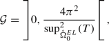  (8.3)

  then ${{\mathcal {A}}}$ also has an eigenvalue in ${\mathcal {G}}$.

• (b) If there exists $\mu \ge 1$ such that $-\bar{{\mathcal {D}}}^2 - \frac{1}{\mu }\bar{{\mathcal {B}}}$ possesses an eigenvalue in the principal gap

  

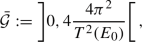  (8.4)

  then $\bar{{\mathcal {A}}}$ also has an eigenvalue in $\bar{{\mathcal {G}}}$.

Proof

For part (a), ${{\mathcal {B}}}\ge 0$ (in the sense of quadratic forms, see [29, Definition 5.11]) and $\frac{1}{\mu }\le 1$ yield $-{{\mathcal {D}}}^2-\frac{1}{\mu }{{\mathcal {B}}}\ge {{\mathcal {A}}}$. Note that $-{{\mathcal {D}}}^2-\frac{1}{\mu }{{\mathcal {B}}}$ is self-adjoint since ${{\mathcal {D}}}^2$ is self-adjoint and ${{\mathcal {B}}}$ is bounded and symmetric. By assuming the existence of an eigenvalue of $-{{\mathcal {D}}}^2-\frac{1}{\mu }{{\mathcal {B}}}$ in the principal gap, we have $-{{\mathcal {D}}}^2 - \frac{1}{\mu }{{\mathcal {B}}}<\frac{4\pi ^2}{\sup ^2(T)} \mathrm {id}$, where < is defined as $\not \ge$. Thus, transitivity yields ${{\mathcal {A}}}<\frac{4\pi ^2}{\sup ^2(T)} \mathrm {id}$, which means that

cf. [29]. Since ${{\mathcal {A}}}$ is restricted to functions odd in v here, Theorem 7.5 (see also Remark 7.6 (a)) implies $\sigma ({{\mathcal {A}}})\subset ]0,\infty [$, i.e., we obtain $\sigma ({{\mathcal {A}}})\cap {\mathcal {G}}\ne \emptyset$. By Theorem 5.9 every element of the spectrum of ${{\mathcal {A}}}$ within ${\mathcal {G}}$ has to be an eigenvalue of ${\mathcal {A}}$; see also [58, Theorem XIII.1].

The proof of part (b) is analogous; the positivity of the resulting eigenvalue is ensured by Theorem 7.9. Recall however that we have restricted the operators onto $\bar{{\mathcal {H}}}$ in the planar setting and the essential spectrum of $\bar{{\mathcal {A}}}$ is given by (5.25). In particular, the bottom of the essential spectrum is $4\frac{4\pi ^2}{T^2(E_0)}$. $\square$

We now investigate the properties of $Q_\lambda$ and $\bar{Q}_\lambda$ for fixed $\lambda \in \rho (-{{\mathcal {D}}}^2)$ and $\lambda \in \rho (-\bar{{\mathcal {D}}}^2)$ respectively. As usual, $\rho {:}{=}{\mathbb {C}}\setminus \sigma$ denotes the resolvent set. Since all involved operators are self-adjoint, we always restrict ourselves to real $\lambda$.

Lemma 8.3

The operators $Q_\lambda :H^{odd}\rightarrow H^{odd}$ and $\bar{Q}_\lambda :\bar{{\mathcal {H}}}\rightarrow \bar{{\mathcal {H}}}$ are both linear, continuous, and compact.

Proof

We only prove the claim for $Q_\lambda$ as the claim for $\bar{Q}_\lambda$ follows analogously. Linearity is obvious, continuity follows by Lemma 4.3 together with the boundedness of the resolvent operator $R_{-{{\mathcal {D}}}^2}(\lambda )$ in the case $\lambda \in \rho (-{{\mathcal {D}}}^2)$. The compactness of $Q_\lambda$ is equivalent to the relative $(-{{\mathcal {D}}}^2)$-compactness of ${{\mathcal {B}}}$, see Theorem 5.9 (and [29, Definition 14.1]). $\square$

Since $\text {im}(Q_\lambda )\subset \text {im}({\mathcal {B}})$, it is of interest to characterize measurable functions $G:[0,\infty [\rightarrow {\mathbb {R}}$ such that $g(r,w,L) = \vert \varphi '(E,L)\vert \,w\,G(r)\in H$; recall the definition of ${{\mathcal {B}}}$ in (4.4).

Lemma 8.4

• (a) If a spherically symmetric $g:\Omega _0\rightarrow {\mathbb {R}}$ is of the form $g(r,w,L) = \vert \varphi '(E,L)\vert \,w\,G(r)$, then

  $$\begin{aligned} g\in H\Leftrightarrow \int _0^\infty r^2\,\rho _0(r)\,G^2(r) \mathop {}\!\mathrm {d}r < \infty . \end{aligned}$$

  In particular, by the boundedness of $\rho _0$, $\int _0^\infty r^2\,G^2(r) \mathop {}\!\mathrm {d}r < \infty$ implies $g\in H$.

• (b) If $g:{\bar{\Omega }}_0\rightarrow {\mathbb {R}}$ is of the form $g(x,v) = \vert \varphi '(E,\bar{v})\vert \,v_1\,G(x)$, then

  $$\begin{aligned} g\in {\bar{H}}\Leftrightarrow \int _{{\mathbb {R}}} \rho _0(x)\,G^2(x) \mathop {}\!\mathrm {d}x < \infty . \end{aligned}$$

  In particular, by the boundedness of $\rho _0$, $\int _{{\mathbb {R}}} G^2(x) \mathop {}\!\mathrm {d}x < \infty$ implies $g\in {\bar{H}}$. Furthermore, g is odd in x if and only if G is odd in x.

Proof

As to part (a), Fubini’s theorem shows that $g\in H$ is equivalent to

$$\begin{aligned} \infty > \Vert g\Vert _{H}^2&= 4\pi ^2 \int _0^\infty G^2(r) \int _0^\infty \int _{{\mathbb {R}}} w^2\,\vert \varphi '(E,L)\vert \mathop {}\!\mathrm {d}w \mathop {}\!\mathrm {d}L \mathop {}\!\mathrm {d}r \\&= 4\pi \int _0^\infty r^2\,\rho _0(r)\,G^2(r)\mathop {}\!\mathrm {d}r, \end{aligned}$$

where we used (4.5) for the last equality.

Similarly, for $g:{\bar{\Omega }}_0\rightarrow {\mathbb {R}}$,

$$\begin{aligned} \Vert g\Vert _{{\bar{H}}}^2&= \int _{{\mathbb {R}}}G^2(x)\int _{{\mathbb {R}}^3}v_1^2\, \vert \varphi '(E,\bar{v})\vert \mathop {}\!\mathrm {d}v\mathop {}\!\mathrm {d}x = \int _{{\mathbb {R}}}\rho _0(x)\,G^2(x)\mathop {}\!\mathrm {d}x \end{aligned}$$

by (4.12), and part (b) follows. $\square$

Let

$$\begin{aligned} S&{:}{=}\left\{ r\ge 0\mid \rho _0(r)\ne 0 \right\} \subset [0,R_0[, \end{aligned}$$

(8.5)

$$\begin{aligned} \bar{S}&{:}{=}\left\{ x\in {\mathbb {R}}\mid \rho _0(x)\ne 0 \right\} =]-R_0,R_0[, \end{aligned}$$

(8.6)

denote the spatial support of the respective steady states. Based on the previous lemma, it is natural to introduce the spaces

$$\begin{aligned} {\mathcal {F}}&{:}{=}\left\{ G:S\rightarrow {\mathbb {R}}\text { measurable}\mid \int _S r^2\,\rho _0(r)\,G^2(r)\mathop {}\!\mathrm {d}r < \infty \right\} , \end{aligned}$$

(8.7)

$$\begin{aligned} {\mathcal {F}}_1&{:}{=}\left\{ G:S\rightarrow {\mathbb {R}}\text { measurable}\mid \int _S r^2\,G^2(r)\mathop {}\!\mathrm {d}r < \infty \right\} \subset {\mathcal {F}}, \end{aligned}$$

(8.8)

and similarly

$$\begin{aligned} \bar{{\mathcal {F}}}&{:}{=}\left\{ G:\bar{S}\rightarrow {\mathbb {R}}\text { measurable and odd}\mid \int _{\bar{S}} \rho _0(x) G^2(x)\mathop {}\!\mathrm {d}x < \infty \right\} , \end{aligned}$$

(8.9)

$$\begin{aligned} \bar{{\mathcal {F}}}_1&{:}{=}\left\{ G:\bar{S}\rightarrow {\mathbb {R}}\text { measurable and odd}\mid \int _{\bar{S}} G^2(x)\mathop {}\!\mathrm {d}x < \infty \right\} \subset \bar{{\mathcal {F}}}. \end{aligned}$$

(8.10)

We treat ${\mathcal {F}}, {\mathcal {F}}_1, \bar{{\mathcal {F}}}, \bar{{\mathcal {F}}}_1$ as (subsets of weighted) $L^2$-spaces, i.e., we identify functions which are equal a.e. on S or $\bar{S}$ respectively. Their norms $\Vert \cdot \Vert _{{\mathcal {F}}}$, $\Vert \cdot \Vert _{{\mathcal {F}}_1}$, $\Vert \cdot \Vert _{\bar{{\mathcal {F}}}}$, $\Vert \cdot \Vert _{\bar{{\mathcal {F}}}_1}$ and scalar products $\langle \cdot ,\cdot \rangle _{{\mathcal {F}}}$, $\langle \cdot ,\cdot \rangle _{{\mathcal {F}}_1}$, $\langle \cdot ,\cdot \rangle _{\bar{{\mathcal {F}}}}$, $\langle \cdot ,\cdot \rangle _{\bar{{\mathcal {F}}}_1}$ are defined accordingly.

Definition & Remark 8.5

(The Mathur operators)

• (a) Let $G\in {\mathcal {F}}$ and define $g(r,w,L){:}{=}\vert \varphi '(E,L)\vert \,w\,G(r)$. Then by Lemma 8.4, $g\in H^{odd}$. Since $Q_\lambda g \in \mathrm {im}({{\mathcal {B}}})$, there exists $F\in {\mathcal {F}}$ such that $(Q_\lambda g)(r,w,L)=\vert \varphi '(E,L)\vert \,w\,F(r)$ for a.e. $(r,w,L)\in \Omega _0^r$, and F is uniquely determined by G. This defines a map

  $$\begin{aligned} {\mathcal {M}}_\lambda :{\mathcal {F}}\rightarrow {\mathcal {F}},~ G\mapsto F . \end{aligned}$$

• (b) Let $G\in \bar{{\mathcal {F}}}$ and define $g(x,v){:}{=}\vert \varphi '(E,\bar{v})\vert \, v_1\, G(x)$. Then by Lemma 8.4, $g\in \bar{{\mathcal {H}}}$. Since $\bar{Q}_\lambda g\in \mathrm {im}(\bar{{\mathcal {B}}})$, there exists a unique $F\in \bar{{\mathcal {F}}}$ such that $(\bar{Q}_\lambda g)(x,v)=\vert \varphi '(E,\bar{v})\vert \, v_1\, F(x)$ for a.e. $(x,v)\in {\bar{\Omega }}_0$. This defines a map

  $$\begin{aligned} \bar{{\mathcal {M}}}_\lambda :\bar{{\mathcal {F}}}\rightarrow \bar{{\mathcal {F}}},~ G\mapsto F . \end{aligned}$$

These operators were introduced by Mathur [52], and we refer to ${\mathcal {M}}_\lambda$ $(\bar{{\mathcal {M}}}_\lambda )$ as the (planar) Mathur operator. The following key integral kernel representation of ${\mathcal {M}}_\lambda$ is essentially also contained in [52].

Proposition 8.6

For any $G\in {\mathcal {F}}$,

$$\begin{aligned} ({\mathcal {M}}_\lambda G)(r)= \int _S K_\lambda (r,\sigma )\,G(\sigma )\mathop {}\!\mathrm {d}\sigma \end{aligned}$$

(8.11)

for a.e. $r\in S$, where

$$\begin{aligned}&K_\lambda (r,\sigma ){:}{=}\frac{32\pi ^2}{r^2} \sum _{k=1}^\infty \int _{\Omega _0^{EL}(r)\cap \Omega _0^{EL}(\sigma )} \frac{\vert \varphi '(E,L)\vert }{T(E,L)} \nonumber \\ {}&\quad \times \frac{\sin (2\pi k\theta (r,E,L))\sin (2\pi k\theta (\sigma ,E,L))}{\frac{4\pi ^2}{T(E,L)^2}k^2-\lambda }\mathop {}\!\mathrm {d}(E,L) \end{aligned}$$

(8.12)

for $r,\sigma >0$,

$$\begin{aligned} \Omega _0^{EL}(r) {:}{=}\left\{ (E,L)\in \mathring{\Omega }_0^{EL} \mid r_-(E,L)<r<r_+(E,L) \right\} , \quad r>0, \end{aligned}$$

and $\theta$ is defined in (5.3). Moreover, the map $]0,\infty [^2\ni (r,\sigma )\mapsto K_\lambda (r,\sigma )\in {\mathbb {R}}$ is continuous.

Proof

To apply $Q_\lambda$ on $g\in H^{odd}$ defined by $g(r,w,L)=\vert \varphi '(E,L)\vert \,w\,G(r)$, we first have to apply the resolvent operator $R_{-{{\mathcal {D}}}^2}(\lambda )$. For this purpose we expand g in its $\theta$-Fourier series (recall that g is odd w.r.t. v):

$$\begin{aligned} g(\theta ,E,L) = \sum _{k=1}^\infty b_k(E,L) \sin (2\pi k\theta ), \end{aligned}$$

(8.13)

where

$$\begin{aligned} b_k(E,L) {:}{=}2\int _0^1 g(\theta ,E,L) \sin (2\pi k\theta )\mathop {}\!\mathrm {d}\theta ,\qquad (E,L)\in \mathring{\Omega }_0^{EL}. \end{aligned}$$

(8.14)

Using (8.13)—which holds as a limit in $H$—now allows us to apply the resolvent operator:

$$\begin{aligned} \left( R_{-{{\mathcal {D}}}^2}(\lambda ) g\right) (\theta ,E,L) = \sum _{k=1}^\infty \frac{1}{\frac{4\pi ^2}{T(E,L)^2}k^2-\lambda } b_k(E,L) \sin (2\pi k\theta ) \end{aligned}$$

(8.15)

as a limit in $H$; the representation (8.15) of the resolvent follows by Corollary 5.4.

To apply ${{\mathcal {B}}}$, we change variables via (5.3) and get

$$\begin{aligned} b_k(E,L)&= 4\int _0^{\frac{1}{2}} g(\theta ,E,L) \sin (2\pi k\theta ) \mathop {}\!\mathrm {d}\theta \nonumber \\&= 4 \frac{\vert \varphi '(E,L)\vert }{T(E,L)} \int _{r_-(E,L)}^{r_+(E,L)} G(r) \sin (2\pi k\theta (r,E,L)) \mathop {}\!\mathrm {d}r. \end{aligned}$$

(8.16)

As for ${{\mathcal {B}}}$, observe that for every $f\in H^{odd}$,

$$\begin{aligned} \left( {{\mathcal {B}}}f\right) (r,w,L)&= 8\pi ^2 \vert \varphi '(E,L)\vert \frac{w}{r^2}\int _{\Omega _0^{EL}(r)} f(r,\sqrt{2{\tilde{E}}-2\Psi _{{\tilde{L}}}(r)},{\tilde{L}})\mathop {}\!\mathrm {d}({\tilde{E}},{\tilde{L}}). \end{aligned}$$

(8.17)

Inserting $f=R_{-{{\mathcal {D}}}^2}(\lambda )g$ yields the following for the integral in (8.17) for $r>0$:

$$\begin{aligned}&\int _{\Omega _0^{EL}(r)} \left( R_{-{{\mathcal {D}}}^2}(\lambda )g\right) (\theta (r,E,L),E,L)\mathop {}\!\mathrm {d}(E,L) \nonumber \\ {}&\quad = 4 \int _{\Omega _0^{EL}(r)} \sum _{k=1}^\infty \frac{\vert \varphi '(E,L)\vert }{T(E,L)} \frac{\sin (2\pi k\theta (r,E,L))}{\frac{4\pi ^2}{T(E,L)^2}k^2-\lambda }\nonumber \\ {}&\qquad \times \int _{r_-(E,L)}^{r_+(E,L)}G(\sigma ) \sin (2\pi k\theta (\sigma ,E,L)) \mathop {}\!\mathrm {d}\sigma \mathop {}\!\mathrm {d}(E,L) \nonumber \\ {}&\quad = 4\int _0^\infty G(\sigma ) \sum _{k=1}^\infty \int _{\Omega _0^{EL}(r)\cap \Omega _0^{EL}(\sigma )}\frac{\vert \varphi '(E,L)\vert }{T(E,L)}\nonumber \\ {}&\qquad \times \frac{\sin (2\pi k\theta (r,E,L))\sin (2\pi k\theta (\sigma ,E,L))}{\frac{4\pi ^2}{T(E,L)^2}k^2-\lambda }\mathop {}\!\mathrm {d}(E,L)\mathop {}\!\mathrm {d}\sigma , \end{aligned}$$

(8.18)

where we used (8.15), (8.16), and Fubini’s theorem. Note that we switched the infinite sum with the $\sigma$-integral and then with the (E, L)-integral in the last equality. Switching with the $\sigma$-integral is verified by fixing $(E,L)\in \Omega _0^{EL}(r)$ and observing that the weight $r^2\rho _0(r)$ is bounded away from 0 on $[r_-(E,L),r_+(E,L)]$ if $L>0$, i.e., G is integrable over $[r_-(E,L),r_+(E,L)]$. Furthermore, recall that the distance of $\lambda$ to the essential spectrum of $-{{\mathcal {D}}}^2$ is positive. The second switch will be justified below. Together with (8.17) we get the desired representation (8.11) of ${\mathcal {M}}_\lambda G$.

To prove the continuity of $(r,\sigma )\mapsto K_\lambda (r,\sigma )$ we first extend the mapping $\theta$ from (5.3) by setting

$$\begin{aligned} \theta (r,E,L){:}{=}0 \text { for } r>0,~(E,L)\in \mathring{\Omega }_0^{EL}\setminus \Omega _0^{EL}(r). \end{aligned}$$

(8.19)

Then

$$\begin{aligned} (r,\sigma )\mapsto \frac{\vert \varphi '(E,L)\vert }{T(E,L)} \frac{\sin (2\pi k\theta (r,E,L))\sin (2\pi k\theta (\sigma ,E,L))}{\frac{4\pi ^2}{T(E,L)^2}k^2-\lambda } \end{aligned}$$

(8.20)

is continuous on $]0,\infty [^2$ for every $k\in {\mathbb {N}}$ and $(E,L)\in \mathring{\Omega }_0^{EL}$. Moreover, there exists a constant $C>0$ depending only on $\lambda$ such that

$$\begin{aligned}&\left| \sum _{k=1}^n\frac{\vert \varphi '(E,L)\vert }{T(E,L)} \frac{\sin (2\pi k\theta (r,E,L))\sin (2\pi k\theta (\sigma ,E,L))}{\frac{4\pi ^2}{T(E,L)^2}k^2-\lambda } \right| \nonumber \\&\quad \le \frac{\vert \varphi '(E,L)\vert }{\inf _{\mathring{\Omega }_0^{EL}}(T)} C\sum _{k=1}^n\frac{1}{k^2}\le \frac{\vert \varphi '(E,L)\vert }{\inf _{\mathring{\Omega }_0^{EL}}(T)}C\frac{\pi ^2}{6} \end{aligned}$$

(8.21)

for $r,\sigma >0$, $(E,L)\in \mathring{\Omega }_0^{EL}$ and $n\in {\mathbb {N}}$; note $\inf _{\mathring{\Omega }_0^{EL}}(T)>0$ by Proposition B.1. This shows that for fixed $(E,L)\in \mathring{\Omega }_0^{EL}$ the limit

$$\begin{aligned} \sum _{k=1}^\infty \frac{\vert \varphi '(E,L)\vert }{T(E,L)} \frac{\sin (2\pi k\theta (r,E,L))\sin (2\pi k\theta (\sigma ,E,L))}{\frac{4\pi ^2}{T(E,L)^2}k^2-\lambda } \end{aligned}$$

(8.22)

exists uniformly in $r,\sigma >0$ and (8.22) defines a continuous function in $(r,\sigma )$. Moreover, since $\vert \varphi '\vert$ is integrable over $\Omega _0^{EL}$ by (2.5) (after changing variables via (5.2)), we conclude that

$$\begin{aligned} \int _{\Omega _0^{EL}}\sum _{k=1}^\infty \frac{\vert \varphi '(E,L)\vert }{T(E,L)} \frac{\sin (2\pi k\theta (r,E,L))\sin (2\pi k\theta (\sigma ,E,L))}{\frac{4\pi ^2}{T(E,L)^2}k^2-\lambda } \mathop {}\!\mathrm {d}(E,L) \end{aligned}$$

(8.23)

is also continuous in $r,\sigma >0$. The dominated convergence theorem and (8.21) yield that we can switch the order of the integral and the infinite sum in (8.23), i.e., it follows that the kernel $K_\lambda$ is indeed continuous on $]0,\infty [^2$. $\square$

In the planar case, we can prove an analogous statement by exactly the same method.

Proposition 8.7

For any $G\in \bar{{\mathcal {F}}}$,

$$\begin{aligned} \bar{{\mathcal {M}}}_\lambda (G)(x)= \int _{\bar{S}} {\bar{K}}_\lambda (x,y)\,G(y)\,\mathop {}\!\mathrm {d}y \end{aligned}$$

(8.24)

for a.e. $x\in \bar{S}$, where

$$\begin{aligned} {\bar{K}}_\lambda (x,y){:}{=}32\pi \sum _{k=1}^\infty \int _{{\bar{\Omega }}_0^{E}(x)\cap {\bar{\Omega }}_0^{E}(y)} \frac{\vert \alpha '(E)\vert }{T(E)} \frac{\sin (4\pi k\theta (x,E))\sin (4\pi k\theta (y,E))}{\frac{4\pi ^2}{T(E)^2}(2k)^2-\lambda }\mathop {}\!\mathrm {d}E\end{aligned}$$

(8.25)

for $x,y\in {\mathbb {R}}$,

$$\begin{aligned} {\bar{\Omega }}_0^{E}(x) {:}{=}\left\{ E\in ]U_0(0),E_0[\, \mid x_-(E)<x<x_+(E) \right\} , \quad x\in {\mathbb {R}}, \end{aligned}$$

and $\theta$ is defined in (5.18). Moreover, ${\mathbb {R}}^2\ni (x,y)\mapsto {\bar{K}}_\lambda (x,y)\in {\mathbb {R}}$ is a bounded continuous function. Here $\alpha$ is the microscopic equation of state related to $f_0$ via (2.14).

Proof

Except for obvious changes the proof is almost identical to the one of Proposition 8.6. The resolvent operator reads

$$\begin{aligned} \left( R_{-\bar{{\mathcal {D}}}^2}(\lambda ) g\right) (\theta ,E, \bar{v}) = \sum _{k=1}^\infty \frac{1}{\frac{4\pi ^2}{T(E)^2} (2k)^2-\lambda } b_k(E,\bar{v}) \sin (4\pi k\theta ), \end{aligned}$$

(8.26)

where

$$\begin{aligned} b_k(E,\bar{v}) {:}{=}&2\int _0^1 g(\theta ,E,\bar{v}) \sin (4\pi k\theta )\mathop {}\!\mathrm {d}\theta \;\; \text{ and } \;\; \nonumber \\g(\theta ,E,\bar{v}) =&\sum _{k=1}^\infty b_k(E,\bar{v}) \sin (4\pi k\theta ) \end{aligned}$$

(8.27)

is the $\theta$-Fourier series expansion of $g\in \bar{{\mathcal {H}}}$ defined by $g(x,v)=\vert \varphi '(E,\bar{v})\vert \,v_1\,G(x)$. Recall that g is odd in x and $v_1$, so the Fourier series does not contain any $\cos$-terms nor $\sin (2\pi k\cdot )$-terms with odd k, see also Remark 5.18. We then follow the proof above and note that the $\bar{v}$-integral can be computed explicitly since $\varphi '(E,\bar{v})=\alpha '(E)\,\beta (\bar{v})$. $\square$

For the spectral analysis it is beneficial to treat ${\mathcal {M}}_\lambda$ ($\bar{{\mathcal {M}}}_\lambda$) as an operator on ${\mathcal {F}}_1$ ($\bar{{\mathcal {F}}}_1$) instead of ${\mathcal {F}}$ ($\bar{{\mathcal {F}}}$), since the Mathur operators are symmetric on the former spaces.

Lemma 8.8

Define ${\mathcal {M}}_\lambda :{\mathcal {F}}_1\rightarrow {\mathcal {F}}_1$ and $\bar{{\mathcal {M}}}_\lambda :\bar{{\mathcal {F}}}_1\rightarrow \bar{{\mathcal {F}}}_1$ by (8.11) and (8.24) respectively. These operators are well-defined, linear, bounded, and self-adjoint. Furthermore, they are Hilbert-Schmidt operators and therefore compact, see e.g. [59, Theorems VI.22 and VI.23].

Proof

For all the claimed properties except of the self-adjointness, it suffices to show that the integrals

$$\begin{aligned} \int _S\int _S \frac{r^2}{\sigma ^2} K_\lambda ^2(r,\sigma )\mathop {}\!\mathrm {d}\sigma \mathop {}\!\mathrm {d}r, \ \ \int _{\bar{S}}\int _{\bar{S}}{\bar{K}}_\lambda ^2(x,y)\mathop {}\!\mathrm {d}y\mathop {}\!\mathrm {d}x \end{aligned}$$

(8.28)

are finite, since for $G\in {\mathcal {F}}_1$ we have by Cauchy-Schwarz

$$\begin{aligned} \Vert {\mathcal {M}}_\lambda G\Vert _{{\mathcal {F}}_1}^2&= \int _S r^2\,\left( \int _S K_\lambda (r,\sigma )\,G(\sigma )\mathop {}\!\mathrm {d}\sigma \right) ^2\mathop {}\!\mathrm {d}r\\&\le \Vert G\Vert _{{\mathcal {F}}_1}^2 \int _S\int _S \frac{r^2}{\sigma ^2} K_\lambda ^2(r,\sigma )\mathop {}\!\mathrm {d}\sigma \mathop {}\!\mathrm {d}r; \end{aligned}$$

a similar estimate holds in the planar case.

If the spherically symmetric steady state is of polytropic form (2.2) with $L_0>0$, then the spatial support is bounded away from 0 due to the presence of an inner vacuum region. In this case (8.28) is obviously finite since the integrand is bounded on $S^2$. In the planar setting, the finiteness of the second integral in (8.28) follows similarly by the boundedness of the integrand as there are no singular terms in (8.25). The finiteness of the first integral in (8.28) for the remaining radial steady states is more challenging but will be shown below. Before that, observe that the symmetry of ${\mathcal {M}}_\lambda :{\mathcal {F}}_1\rightarrow {\mathcal {F}}_1$ follows from

$$\begin{aligned} \langle {\mathcal {M}}_\lambda G,F\rangle _{{\mathcal {F}}} = \int _S\int _Sr^2K_\lambda (r,\sigma )\,G(\sigma )\,F(r)\mathop {}\!\mathrm {d}\sigma \mathop {}\!\mathrm {d}r \end{aligned}$$

and the symmetry of $r^2K_\lambda (r,\sigma )$ in $(r,\sigma )$. The planar case is obvious.

Now consider a radial steady state of King type (2.3) or a polytrope (2.2) with $L_0=0$. In particular, $\varphi (E,L)=\varphi (E)$ in both cases, i.e., the steady state is isotropic. For every $f\in L^2(S\times S)$,

$$\begin{aligned}&\left| \int _S\int _S\frac{r}{\sigma }K_\lambda (r,\sigma )f(r,\sigma )\mathop {}\!\mathrm {d}\sigma \mathop {}\!\mathrm {d}r\right| \\ {}&\quad \le 32\pi ^2\sum _{k=1}^\infty \int _{\Omega _0^{EL}}\frac{\vert \varphi '(E)\vert }{T(E,L)}\frac{1}{\frac{4\pi ^2}{T(E,L)^2}k^2-\lambda }\\&\qquad \times \int _{r_-(E,L)}^{r_+(E,L)}\int _{r_-(E,L)}^{r_+(E,L)}\left| \frac{\sin (2\pi k\theta (r,E,L))}{r}\frac{\sin (2\pi k\theta (\sigma ,E,L))}{\sigma }f(r,\sigma )\right| \mathop {}\!\mathrm {d}\sigma \mathop {}\!\mathrm {d}r\mathop {}\!\mathrm {d}(E,L)\\ {}&\quad \le 32\pi ^2\Vert f\Vert _{L^2(S\times S)}\sum _{k=1}^\infty \int _{\Omega _0^{EL}}\frac{\vert \varphi '(E)\vert }{T(E,L)}\\ {}&\qquad \times \frac{1}{\frac{4\pi ^2}{T(E,L)^2}k^2-\lambda }\int _{r_-(E,L)}^{r_+(E,L)}\frac{\sin ^2(2\pi k\theta (r,E,L))}{r^2}\mathop {}\!\mathrm {d}r\mathop {}\!\mathrm {d}(E,L) \end{aligned}$$

by inserting (8.12); the following calculations will show that we can switch the infinite sum with the integrals. Thus,

$$\begin{aligned}&\int _S\int _S\frac{r^2}{\sigma ^2} K_\lambda ^2(r,\sigma )\mathop {}\!\mathrm {d}\sigma \mathop {}\!\mathrm {d}r\\&\quad \le 32\pi ^2\sum _{k=1}^\infty \int _{\Omega _0^{EL}}\frac{\vert \varphi '(E)\vert }{T(E,L)}\frac{1}{\frac{4\pi ^2}{T(E,L)^2}k^2-\lambda }\\&\qquad \quad \times \int _{r_-(E,L)}^{r_+(E,L)}\frac{\sin ^2(2\pi k\theta (r,E,L))}{r^2}\mathop {}\!\mathrm {d}r\mathop {}\!\mathrm {d}(E,L)\\&\quad \le \frac{32\pi ^2}{\inf _{\mathring{\Omega }_0^{EL}}(T)}\sum _{k=1}^\infty \int _{\Omega _0^{EL}}\frac{\vert \varphi '(E)\vert }{\frac{4\pi ^2}{T(E,L)^2}k^2-\lambda }\int _{r_-(E,L)}^{r_+(E,L)}\frac{\mathop {}\!\mathrm {d}r}{r^2} \mathop {}\!\mathrm {d}(E,L)\\&\quad \le C\int _{\Omega _0^{EL}} \frac{\vert \varphi '(E)\vert }{r_-(E,L)}\mathop {}\!\mathrm {d}(E,L) \end{aligned}$$

for some constant $C>0$ depending on the steady state and $\lambda$; note that T is bounded away from 0 by Proposition B.1 and that the distance between $\lambda$ and the spectrum of $-{{\mathcal {D}}}^2$ is positive. To show that the latter integral is finite, recall that $r_-(E,L)$ is defined in Lemma 2.1 as a solution of

$$\begin{aligned} E=\Psi _L(r_-(E,L))=U_0(r_-(E,L))+\frac{L}{2r_-^2(E,L)}, \end{aligned}$$

which implies

$$\begin{aligned} \frac{1}{r_-(E,L)}=\frac{\sqrt{2E-2U_0(r_-(E,L))}}{\sqrt{L}}\le \sqrt{2}\frac{\sqrt{E_0-U_0(0)}}{\sqrt{L}}. \end{aligned}$$

Thus,

$$\begin{aligned} \int _{\Omega _0^{EL}} \frac{\vert \varphi '(E)\vert }{r_-(E,L)}\mathop {}\!\mathrm {d}(E,L)\le \sqrt{2E_0-2U_0(0)}\int _0^{L_{max}}\frac{\mathop {}\!\mathrm {d}L}{\sqrt{L}}\;\int _{U_0(0)}^{E_0} \vert \varphi '(E)\vert \mathop {}\!\mathrm {d}E <\infty , \end{aligned}$$

where $L_{max}\in ]0,\infty [$ is the maximal L-value in the steady state support and the finiteness of the latter integral follows since $k>0$ in the polytropic case. We therefore conclude that the first integral in (8.28) is indeed finite. $\square$

In the next lemma we show that ${\mathcal {M}}_\lambda$ ($\bar{{\mathcal {M}}}_\lambda$) map ${\mathcal {F}}$ ($\bar{{\mathcal {F}}}$) into the smaller spaces ${\mathcal {F}}_1$ ($\bar{{\mathcal {F}}}_1$).

Lemma 8.9

${\mathcal {M}}_\lambda ({\mathcal {F}})\subset {\mathcal {F}}_1$ and $\bar{{\mathcal {M}}}_\lambda (\bar{{\mathcal {F}}})\subset \bar{{\mathcal {F}}}_1$.

Proof

Let $F\in {\mathcal {M}}_\lambda ({\mathcal {F}})$, i.e., there exists $G\in {\mathcal {F}}$ such that ${\mathcal {M}}_\lambda G=F$. Define the spherically symmetric functions $f,g:\Omega _0\rightarrow {\mathbb {R}}$ by

$$\begin{aligned}&f(r,w,L)=\vert \varphi '(E,L)\vert \,w\,F(r),\\&g(r,w,L)=\vert \varphi '(E,L)\vert \,w\,G(r),\quad (r,w,L)\in \Omega _0^r. \end{aligned}$$

Lemma 8.4 yields $f,g\in H^{odd}$, and $Q_\lambda g=f$ by the definition of ${\mathcal {M}}_\lambda$, see Definition 8.5. In other words,

$$\begin{aligned}&f(r,w,L)={{\mathcal {B}}}h(r,w,L) = 4\pi ^2\vert \varphi '(E,L)\vert \,\frac{w}{r^2}\\&\quad \int _0^\infty \int _{\mathbb {R}}{\tilde{w}}\,h(r,{\tilde{w}},{\tilde{L}})\mathop {}\!\mathrm {d}{\tilde{w}}\mathop {}\!\mathrm {d}{\tilde{L}},\quad (r,w,L)\in \Omega _0^r, \end{aligned}$$

where $h{:}{=}R_{-{{\mathcal {D}}}^2}(\lambda )g\in \mathrm D({{\mathcal {D}}}^2)\cap H^{odd}$. Using the representation of F provided by the formula above, we arrive at

$$\begin{aligned} \Vert F\Vert _{{\mathcal {F}}_1}^2&=\int _Sr^2\,F^2(r)\mathop {}\!\mathrm {d}r=16\pi ^4\int _S\frac{1}{r^2}\,\left( \int _0^\infty \int _{{\mathbb {R}}}w\,h(r,w,L)\mathop {}\!\mathrm {d}w\mathop {}\!\mathrm {d}L\right) ^2\mathop {}\!\mathrm {d}r\\&\le 16\pi ^4\int _S\frac{1}{r^2}\,\left( \int _0^\infty \int _{\mathbb {R}}w^2\,\vert \varphi '(E,L)\vert \mathop {}\!\mathrm {d}w\mathop {}\!\mathrm {d}L\right) \\&\qquad \times \left( \int _0^\infty \int _{\mathbb {R}}\frac{h^2(r,w,L)}{\vert \varphi '(E,L)\vert } \mathop {}\!\mathrm {d}w\mathop {}\!\mathrm {d}L\right) \mathop {}\!\mathrm {d}r\\&\le C\Vert h\Vert _H^2, \end{aligned}$$

where we used (4.5) and the boundedness of $\rho _0$ in the last inequality. In the planar setting the proof is analogous; apply (4.12) instead of (4.5) for the last step. $\square$

We are now in the position to show the equivalence of the eigenvalues of $Q_\lambda$ ($\bar{Q}_\lambda$) and the ones of the Mathur operator ${{\mathcal {M}}}_\lambda$ ($\bar{{\mathcal {M}}}_\lambda$):

Lemma 8.10

Let $\mu \in {\mathbb {R}}\setminus \{0\}$.

• (a) $\mu$ is an eigenvalue of $Q_\lambda$ if and only if $\mu$ is an eigenvalue of ${\mathcal {M}}_\lambda$. Here, ${\mathcal {M}}_\lambda$ can be seen as an operator ${\mathcal {F}}\rightarrow {\mathcal {F}}$ or ${\mathcal {F}}_1\rightarrow {\mathcal {F}}_1$.

• (b) $\mu$ is an eigenvalue of $\bar{Q}_\lambda$ if and only if $\mu$ is an eigenvalue of $\bar{{\mathcal {M}}}_\lambda$, where $\bar{{\mathcal {M}}}_\lambda$ can be seen as an operator $\bar{{\mathcal {F}}}\rightarrow \bar{{\mathcal {F}}}$ or $\bar{{\mathcal {F}}}_1\rightarrow \bar{{\mathcal {F}}}_1$.

Proof

We only prove part (a), similar arguments apply in the planar setting.

If there exists $g\in H^{odd}$ with $Q_\lambda g= \mu g$, then $g\in \mathrm {im}({{\mathcal {B}}})$ since $\mu \ne 0$. Thus, there exists $G:S\rightarrow {\mathbb {R}}$ such that g is of the form $g(r,w,L)=\vert \varphi '(E,L)\vert \,w\,G(r)$, and $G\in {\mathcal {F}}$ by Lemma 8.4. Using Definition 8.5, the eigenvalue equation becomes

$$\begin{aligned} \vert \varphi '(E,L)\vert \,w\,{\mathcal {M}}_\lambda G(r) = \mu \,\vert \varphi '(E,L)\vert \,w\,G(r),\qquad (r,w,L)\in \Omega _0^r. \end{aligned}$$

(8.29)

Hence, ${\mathcal {M}}_\lambda G=\mu G$. In particular, $G\in {\mathcal {F}}_1$ by Lemma 8.9.

Conversely, let $G\in {\mathcal {F}}$ (recall ${\mathcal {F}}_1\subset {\mathcal {F}}$) be such that ${\mathcal {M}}_\lambda G=\mu G$ and define $g(r,w,L)=\vert \varphi '(E,L)\vert \,w\,G(r)$. Then $g\in H^{odd}$ and (8.29) holds true. $\square$

Since ${\mathcal {M}}_\lambda :{\mathcal {F}}_1\rightarrow {\mathcal {F}}_1$ ($\bar{{\mathcal {M}}}_\lambda :\bar{{\mathcal {F}}}_1\rightarrow \bar{{\mathcal {F}}}_1$) is a symmetric and compact Hilbert-Schmidt operator by Lemma 8.8, the spectrum of ${\mathcal {M}}_\lambda$ is real and its largest element is given by

$$\begin{aligned} M_\lambda {:}{=}\sup \left\{ \langle G,{\mathcal {M}}_\lambda G\rangle _{{\mathcal {F}}_1} \mid G\in {\mathcal {F}}_1,\,\Vert G\Vert _{{\mathcal {F}}_1}=1\right\} . \end{aligned}$$

(8.30)

Similarly, the largest element in the spectrum of $\bar{{\mathcal {M}}}_\lambda$ is

$$\begin{aligned} \bar{M}_\lambda {:}{=}\sup \left\{ \langle G,\bar{{\mathcal {M}}}_\lambda G\rangle _{\bar{{\mathcal {F}}}_1} \mid G\in \bar{{\mathcal {F}}}_1,\,\Vert G\Vert _{\bar{{\mathcal {F}}}_1}=1\right\} . \end{aligned}$$

(8.31)

Furthermore, if $M_\lambda \ne 0$ ($\bar{M}_\lambda \ne 0$), then $M_\lambda$ ($\bar{M}_\lambda$) is actually an eigenvalue of ${\mathcal {M}}_\lambda$ ($\bar{{\mathcal {M}}}_\lambda$).

Theorem 8.11

(Criterion for the existence of oscillating modes)

• (a) Let $f_0$ be a radial steady state of the form (2.2) or (2.3). Then the linearized operator ${{\mathcal {A}}}$ possesses an eigenvalue in the principal gap ${\mathcal {G}}$—defined in (8.3)—with associated eigenfunction odd in v if and only if there exists a $\lambda \in {\mathcal {G}}$ such that

  $$\begin{aligned} M_\lambda \ge 1. \end{aligned}$$

  (8.32)

• (b) Let $f_0$ be a planar steady state as specified in Sect. 2.2. Then the linearized operator $\bar{{\mathcal {A}}}$ possesses an eigenvalue in the principal gap $\bar{{\mathcal {G}}}$—defined in (8.4)—with associated eigenfunction odd in $v_1$ and x if and only if there exists a $\lambda \in \bar{{\mathcal {G}}}$ such that

  $$\begin{aligned} \bar{M}_\lambda \ge 1. \end{aligned}$$

  (8.33)

Proof of part (a)

If $\lambda \in {\mathcal {G}}$ is an eigenvalue of ${{\mathcal {A}}}$ (restricted to $H^{odd}$, i.e., functions in the spherically symmetric, weighted $L^2$-space $H$ which are odd in v), then 1 is an eigenvalue of $Q_\lambda$ by Lemma 8.1. Thus, Lemma 8.10 yields that 1 is also an eigenvalue of ${\mathcal {M}}_\lambda :{\mathcal {F}}_1\rightarrow {\mathcal {F}}_1$, which implies $M_\lambda \ge 1$.

Conversely, if there exists $\lambda \in {\mathcal {G}}$ such that $M_\lambda \ge 1$, then ${\mathcal {M}}_\lambda$ has an eigenvalue $\mu \ge 1$. Lemma 8.10 implies that $\mu$ is also an eigenvalue of $Q_\lambda$, and therefore $\lambda$ is an eigenvalue of $-{{\mathcal {D}}}^2-\frac{1}{\mu }{{\mathcal {B}}}$ by Lemma 8.1. Using Lemma 8.2, we conclude that ${{\mathcal {A}}}$ indeed has an eigenvalue in the principal gap ${\mathcal {G}}$. $\square$

Proof of part (b)

The proof is analogous to the radial setting and uses the planar statements of Lemmas 8.1, 8.2, and 8.10. However, recall that we restricted $\bar{{\mathcal {A}}}$ to $\bar{{\mathcal {H}}}$, i.e., functions odd in $v_1$ and x, in the planar setting, which causes the top of the principal gap $\bar{{\mathcal {G}}}$ to quadruple, see (8.4) and also Theorem 5.19. $\square$

Before verifying these criteria for selected steady states, we state some properties of $M_\lambda$ and $\bar{M}_\lambda$.

Remark 8.12

(Criterion for the existence of eigenvalues in the principal gap) Using the kernel representation of the radial Mathur operator provided by Proposition 8.6, the associated quadratic form can be rewritten as

$$\begin{aligned}&\langle G,{\mathcal {M}}_\lambda G\rangle _{{\mathcal {F}}_1} = \int _S\int _Sr^2\,K_\lambda (r,\sigma )\,G(r)\,G(\sigma )\mathop {}\!\mathrm {d}\sigma \mathop {}\!\mathrm {d}r\nonumber \\&\quad =32\pi ^2\sum _{k=1}^\infty \int _{\Omega _0^{EL}}\frac{\vert \varphi '(E,L)\vert }{T(E,L)} \frac{1}{\frac{4\pi ^2k^2}{T(E,L)^2}-\lambda } \left( \int _{r_-(E,L)}^{r_+(E,L)}\sin (2\pi k\theta (r,E,L))\,G(r)\nonumber \right. \\&\left. \qquad \mathop {}\!\mathrm {d}r\right) ^2 \mathop {}\!\mathrm {d}(E,L) \end{aligned}$$

(8.34)

for $G\in {\mathcal {F}}_1$. Since $\lambda$ is in the principal gap, the latter integral is obviously non-negative, i.e., the spectrum of the Mathur operator is non-negative as well.

Hence $M_\lambda$ coincides with the operator norm of ${\mathcal {M}}_\lambda$, cf. [29, Theorem 5.14]. Furthermore, $M_\lambda$ increases in $\lambda$, which can for example be seen in the integral (8.34). Theorem 8.11 now allows us to translate the existence of an oscillating mode corresponding to an eigenvalue of ${{\mathcal {A}}}$ in the principal gap into a condition on the size of

$$\begin{aligned} M{:}{=}\sup _{\lambda \in {\mathcal {G}}}M_\lambda =\sup _{\lambda \in {\mathcal {G}}}\Vert {\mathcal {M}}_\lambda \Vert _{{\mathcal {F}}_1\rightarrow {\mathcal {F}}_1}: \end{aligned}$$

(8.35)

• (a) If $M>1$, then ${{\mathcal {A}}}$ possesses at least one eigenvalue in the principal gap.

• (b) If $M<1$, then ${{\mathcal {A}}}$ has no eigenvalues in the principal gap.

• (c) In the case $M=1$, the existence of an eigenvalue of ${{\mathcal {A}}}$ in the principal gap depends on whether or not the supremum (8.35) is attained.

Similar statements hold true in the plane symmetric setting. In particular, the spectrum of $\bar{{\mathcal {M}}}_\lambda :\bar{{\mathcal {F}}}_1\rightarrow \bar{{\mathcal {F}}}_1$ is non-negative, and

$$\begin{aligned} \bar{M}{:}{=}\sup _{\lambda \in \bar{{\mathcal {G}}}}\bar{M}_\lambda =\sup _{\lambda \in \bar{{\mathcal {G}}}}\Vert \bar{{\mathcal {M}}}_\lambda \Vert _{\bar{{\mathcal {F}}}_1\rightarrow \bar{{\mathcal {F}}}_1} \end{aligned}$$

(8.36)

being larger (smaller) than 1 implies the existence one (no) eigenvalue(s) of $\bar{{\mathcal {A}}}$ in the principal gap.

8.2 Examples of linear oscillations

We now apply Theorem 8.11 to give a class of examples of steady states which allow for pulsating modes. A particularly simple-minded approach is to identify steady states for which $M_\lambda$ ($\bar{M}_\lambda$) tends to infinity as $\lambda$ approaches the top of the principal gap.

8.2.1 Linear oscillations in the planar case

In the plane symmetric setting we are able to analytically show the existence of linearly pulsating modes for a large class of steady state models by pursuing the approach discussed above.

Theorem 8.13

Let $f_0$ be a planar steady state of polytropic form (2.18) with $\frac{1}{2}<k\le 1$ or of King type (2.19). Then the associated linearized operator $\bar{{\mathcal {A}}}$—restricted to $\bar{{\mathcal {H}}}$, i.e., functions in ${\bar{H}}$ which are odd in $v_1$ and x—possesses an eigenvalue in the principal gap $\bar{{\mathcal {G}}}=]0,4\frac{4\pi ^2}{T^2(E_0)}[$.

Proof

For $G\in \bar{{\mathcal {F}}}_1$, the quadratic form in (8.31) is

$$\begin{aligned}&\langle G,\bar{{\mathcal {M}}}_\lambda G\rangle _{\bar{{\mathcal {F}}}_1} = \int _{\bar{S}} \int _{\bar{S}} {\bar{K}}_\lambda (x,y)\,G(x)\,G(y)\mathop {}\!\mathrm {d}x\mathop {}\!\mathrm {d}y \nonumber \\&\quad =32\pi \sum _{k=1}^\infty \int _{\bar{S}}\int _{\bar{S}} \int _{{\bar{\Omega }}_0^{E}(x)\cap {\bar{\Omega }}_0^{E}(y)}\nonumber \\&\qquad \times \frac{\vert \alpha '(E)\vert }{T(E)}\frac{\sin (4\pi k\theta (x,E)) \sin (4\pi k\theta (y,E))}{\frac{4\pi ^2}{T(E)^2}(2k)^2-\lambda }\mathop {}\!\mathrm {d}E\,G(x)\,G(y)\mathop {}\!\mathrm {d}x \mathop {}\!\mathrm {d}y \nonumber \\&\quad =32\pi \sum _{k=1}^\infty \int _{U_0(0)}^{E_0}\frac{\vert \alpha '(E)\vert }{T(E)}\frac{1}{\frac{4\pi ^2}{T(E)^2}(2k)^2-\lambda }\nonumber \\&\qquad \times \left( \int _{x_-(E)}^{x_+(E)} \sin (4\pi k\theta (x,E))\,G(x)\mathop {}\!\mathrm {d}x \right) ^2 \mathop {}\!\mathrm {d}E, \end{aligned}$$

(8.37)

see Proposition 8.7 for the definition of ${\bar{K}}_\lambda$. Note that the exchange of the infinite sum and the integration can be justified similarly to the radial case, see for example a related argument in the proof of Proposition 8.6. In particular, for any $\lambda$ in the principal gap, i.e., $0<\lambda <4\frac{4\pi ^2}{T^2(E_0)}$, we conclude that for all non-zero $G\in \bar{{\mathcal {F}}}_1$,

$$\begin{aligned} \bar{M}_\lambda&\ge \frac{\langle G,\bar{{\mathcal {M}}}_\lambda G\rangle _{\bar{{\mathcal {F}}}_1} }{\Vert G\Vert _{\bar{{\mathcal {F}}}_1}^2} \nonumber \\&\ge \frac{32\pi }{\Vert G\Vert _{\bar{{\mathcal {F}}}_1}^2}\int _{U_0(0)}^{E_0}\frac{\vert \alpha '(E)\vert }{T(E)}\frac{1}{\frac{16\pi ^2}{T(E)^2}-\lambda }\left( \int _{x_-(E)}^{x_+(E)} \sin (4\pi \theta (x,E))\,G(x)\mathop {}\!\mathrm {d}x\right) ^2\mathop {}\!\mathrm {d}E. \end{aligned}$$

(8.38)

Consider a neighborhood ${\bar{N}}_\eta {:}{=}[E_0-\eta ,E_0]$ of the cut-off energy $E_0$ for some sufficiently small parameter $0<\eta <E_0-U_0(0)$. By an easy continuity argument we can choose a closed interval ${\bar{I}}\subset ]x_-(E_0),0[=]-R_0,0[$ such that

$$\begin{aligned} \sin (4\pi \theta (x,E)) \ge \frac{1}{2} \quad \text { for } E\in {\bar{N}}_\eta , \ x\in {\bar{I}}, \end{aligned}$$

(8.39)

if $\eta >0$ is sufficiently small, in particular, ${\bar{I}}\subset ]x_-(E),0[$ for $E\in {\bar{N}}_\eta$. Now let

$$\begin{aligned} G:\bar{S}\rightarrow {\mathbb {R}},\quad G(x){:}{=}{\left\{ \begin{array}{ll} 1, &{} x\in {\bar{I}}, \\ -1, &{} -x\in {\bar{I}},\\ 0,&{}\text {else}. \end{array}\right. } \end{aligned}$$

(8.40)

Clearly, G is odd and $G\in \bar{{\mathcal {F}}}_1$ with $\Vert G\Vert _{\bar{{\mathcal {F}}}_1}^2 = 2|{\bar{I}}|$. Moreover,

$$\begin{aligned} \int _{x_-(E)}^{x_+(E)}\sin (4\pi \theta (x,E))\,G(x)\mathop {}\!\mathrm {d}x\ge \vert {\bar{I}}\vert \end{aligned}$$

for any $E\in {\bar{N}}_\eta$; observe that the symmetry of $U_0$ implies $4\pi \theta ([x_-(E),0],E)=[0,\pi ]$ and $4\pi \theta ([0,x_+(E)],E)=[\pi ,2\pi ]$ as well as $\theta (x,E)+\theta (-x,E)=\frac{1}{2}$ for $x\in [x_-(E),0]$, recall the definition (5.18) of $\theta$. Plugging G into (8.38) yields

$$\begin{aligned} \bar{M}_\lambda \ge 16\pi \vert {\bar{I}}\vert \int _{{\bar{N}}_\eta }\frac{\vert \alpha '(E)\vert }{T(E)}\frac{1}{\frac{16\pi ^2}{T(E)^2}-\lambda }\mathop {}\!\mathrm {d}E. \end{aligned}$$

We now let $\lambda \rightarrow \sup \bar{{\mathcal {G}}}=\frac{16\pi ^2}{T(E_0)^2}$—notice that ${\bar{I}}$ is independent of $\lambda$—and conclude by the monotone convergence theorem that

$$\begin{aligned} \limsup _{\lambda \rightarrow \frac{16\pi ^2}{T(E_0)^2}} \bar{M}_\lambda&\ge 16\pi \vert {\bar{I}}\vert \int _{{\bar{N}}_\eta }\frac{\vert \alpha '(E)\vert }{T(E)}\frac{1}{\frac{16\pi ^2}{T(E)^2}-{\frac{16\pi ^2}{T(E_0)^2}}} \mathop {}\!\mathrm {d}E\nonumber \\&=\frac{\vert {\bar{I}}\vert }{\pi }\int _{{\bar{N}}_\eta }\frac{\vert \alpha '(E)\vert }{T(E_0)-T(E)}\,\frac{T(E)\,T(E_0)^2}{T(E)+T(E_0)}\mathop {}\!\mathrm {d}E\nonumber \\&\ge C\int _{{\bar{N}}_\eta }\frac{\vert \alpha '(E)\vert }{T(E_0)-T(E)}\mathop {}\!\mathrm {d}E \end{aligned}$$

(8.41)

for some $C>0$; recall that $T$ is bounded and bounded away from 0 on $[U_0(0),E_0[$ by Proposition 2.8. To show that the latter integral is infinite, we expand the denominator of its integrand. By the mean value theorem, for each $E\in {\bar{N}}_\eta$ there exists $E^*\in {\bar{N}}_\eta$ such that $T(E_0)-T(E)=T'(E^*)\,(E_0-E)$. Since $T'$ is continuous by Lemma 2.6, we obtain $T(E_0)-T(E)\le C\,(E_0-E)$ for $E\in {\bar{N}}_\eta$ and some constant $C>0$ depending on the steady state and $\eta$. Inserting this estimate in (8.41) then yields

$$\begin{aligned} \limsup _{\lambda \rightarrow \frac{16\pi ^2}{T(E_0)^2}} \bar{M}_\lambda&\ge C\int _{{\bar{N}}_\eta }\frac{\vert \alpha '(E)\vert }{E_0-E}\mathop {}\!\mathrm {d}E\\&=C{\left\{ \begin{array}{ll}k\int _{E_0-\eta }^{E_0}\left( E_0-E\right) ^{k-2}\mathop {}\!\mathrm {d}E,&{}\alpha \text { is polytropic with }\frac{1}{2}<k\le 1\\ \int _{E_0-\eta }^{E_0}\frac{e^{E_0-E}}{E_0-E}\mathop {}\!\mathrm {d}E,&{}\alpha \text { is of King type} \end{array}\right. }\\&=\infty . \end{aligned}$$

The claim now follows by part (b) of Theorem 8.11. $\square$

Remark 8.14

• (a) Since $T'>0$ on $]U_0(0),\infty [$, we can not expect to show that the integral (8.41) is infinite for polytropes with exponent $k>1$ by expanding $T$ to higher order.

• (c) For the above proof—and everything in the preceding sections—the exact polytropic (2.18) or King type (2.19) structure of $\alpha$ is not essential. Only the behavior of $\alpha$ near the cut-off energy $E_0$ matters for our argument.

8.2.2 Linear oscillations in the radial case

In order to apply the same idea as in the proof of Theorem 8.13 we need to know where the period function $\mathring{\Omega }_0^{EL}\ni (E,L)\mapsto T(E,L)$ attains its maximal values. This is an involved technical question about the behavior of solutions to semi-linear radial ODEs of Lane-Emden type, which will be rigorously addressed in future work. However, numerical calculations conclusively show that for a wide range of steady states of the form (2.2)–(2.3) the period function has the property that

$$\begin{aligned} \sup _{\mathring{\Omega }_0^{EL}}(T) = T(E_0,L_0), \end{aligned}$$

(8.42)

where $L_0\ge 0$ is the lowest occurring L-value in the steady state support. Note that $T(E_0,L_0)$ may formally not be defined by Definition 2.2, but T can easily be extended to $L=0$ by replacing $\Psi _L$ with $U_0$ in the definition.

In order to Taylor-expand T near its maximal value similar to the planar setting, we further require that

$$\begin{aligned} T\text { is differentiable and }\partial _ET,\,\partial _LT\text { are bounded near }(E_0,L_0). \end{aligned}$$

(8.43)

The latter can be shown by explicitly computing the derivatives of T with respect to E and L, but we choose to leave out the proof of this rather technical statement.

One way to validate (8.42) is to show

$$\begin{aligned} \partial _E T(E,L)&\ge 0, \ \ \partial _L T(E,L) \le 0, \ \quad \text { for } (E,L)\in \mathring{\Omega }_0^{EL}, \end{aligned}$$

(8.44)

and numerical computations indicate that (8.44) is indeed true for a wide range of steady states. We discuss this matter in more detail at the end of Sect. B.3 in the appendix, and give explicit parameters of a steady state for which (8.42) and (8.44) have been verified numerically in Remark 8.16.

Theorem 8.15

Let $f_0$ be a radial steady state of polytropic form (2.2) with parameters $k,l,L_0$ satisfying

$$\begin{aligned} L_0>0,\ \ k>0,\ \ l>-1,\ \ k<l+\frac{7}{2},\ \ k+l+\frac{1}{2}\ge 0,\ \ k+l\le 0. \end{aligned}$$

(8.45)

Assume further that the assumptions (8.42) and (8.43) hold. Then the associated linearized operator ${{\mathcal {A}}}$—restricted to $H^{odd}$, i.e., functions in $H$ which are odd in v—possesses an eigenvalue in the principal gap ${\mathcal {G}}=]0,\frac{4\pi ^2}{\sup ^2(T)}[$.

Proof

Just like in the proof of Theorem 8.13 we can show that

$$\begin{aligned}&M_\lambda \ge \frac{32\pi ^2}{\Vert G\Vert _{{\mathcal {F}}_1}^2} \int _{\Omega _0^{EL}}\frac{\vert \varphi '(E,L)\vert }{T(E,L)}\frac{1}{\frac{4\pi ^2}{T(E,L)^2}-\lambda }\nonumber \\&\qquad \quad \, \times \left( \int _{r_-(E,L)}^{r_+(E,L)} \sin (2\pi k\theta (r,E,L))\,G(r)\mathop {}\!\mathrm {d}r \right) ^2 \mathop {}\!\mathrm {d}(E,L) \end{aligned}$$

(8.46)

for any $G\in {\mathcal {F}}_1\setminus \{0\}$ and $\lambda \in {\mathcal {G}}$. Letting $\lambda \rightarrow \frac{4\pi ^2}{\sup ^2(T)}=\frac{4\pi ^2}{T(E_0,L_0)^2}$, using the monotone convergence theorem, and the boundedness of T from above and away from zero (see Proposition B.1), we conclude that

$$\begin{aligned}&\limsup _{\lambda \rightarrow \frac{4\pi ^2}{\sup ^2(T)}}M_\lambda \ge \frac{C}{\Vert G\Vert _{{\mathcal {F}}_1}^2} \\&\quad \int _{\Omega _0^{EL}} \frac{\vert \varphi '(E,L)\vert }{T(E_0,L_0)-T(E,L)}\left( \int _{r_-(E,L)}^{r_+(E,L)} \sin (2\pi \theta (r,E,L))\,G(r)\mathop {}\!\mathrm {d}r \right) ^2 \mathop {}\!\mathrm {d}(E,L) \end{aligned}$$

for some constant $C>0$ depending on the steady state.

Consider a closed neighborhood $N_\eta$ of the T-maximizer $(E_0,L_0)$ of the form

$$\begin{aligned} N_\eta {:}{=}[E_0-\eta ,E_0]\times [L_0,L_0+\eta ] \end{aligned}$$

for a sufficiently small $\eta >0$ such that $\mathring{N}_\eta \subset \Omega _0^{EL}$. Next, choose a non-empty, closed interval $I\subset S$ such that

$$\begin{aligned} \sin (2\pi \theta (r,E,L)) \ge \frac{1}{2} \quad \text { for } (E,L)\in N_\eta ,~r\in I. \end{aligned}$$

(8.47)

Now let $G{:}{=}\mathbb {1}_I \in {\mathcal {F}}_1$. Analogously to (8.41) we conclude that

$$\begin{aligned} \limsup _{\lambda \rightarrow \frac{4\pi ^2}{T(E_0,L_0)^2}} M_\lambda&\ge C \int _{E_0-\eta }^{E_0}\int _{L_0}^{L_0+\eta }\frac{\vert \varphi '(E,L)\vert }{T(E_0,L_0)-T(E,L)} \mathop {}\!\mathrm {d}L \mathop {}\!\mathrm {d}E. \end{aligned}$$

(8.48)

Taylor-expanding the denominator in this integral gives

$$\begin{aligned} T(E_0,L_0)-T(E,L)&= c_E\,(E_0-E) - c_L\,(L-L_0)\nonumber \\&\quad + o_{(E,L)\rightarrow (E_0,L_0)}\left( \vert (E,L)-(E_0,L_0)\vert \right) , \end{aligned}$$

(8.49)

where we denote $c_E{:}{=}\partial _ET(E_0,L_0),\ c_L{:}{=}\partial _LT(E_0,L_0)<\infty$; recall the assumption (8.43). Thus, after choosing a possibly smaller $\eta$, we use (8.48) and the polytropic structure (2.2) of the steady state model to obtain

$$\begin{aligned} \limsup _{\lambda \rightarrow \frac{4\pi ^2}{T(E_0,L_0)^2}} M_\lambda&\ge C \int _{E_0-\eta }^{E_0}\int _{L_0}^{L_0+\eta } \frac{(E_0-E)^{k-1}(L-L_0)^l}{E_0-E + L-L_0} \mathop {}\!\mathrm {d}L\mathop {}\!\mathrm {d}E \nonumber \\&= C \int _0^\eta \int _0^\eta \frac{x^{k-1}y^l}{x+y} \mathop {}\!\mathrm {d}y\mathop {}\!\mathrm {d}x, \end{aligned}$$

(8.50)

where we used the obvious change of variables $x=E_0-E$ and $y=L-L_0$. The latter integral is infinite precisely when $k+l\le 0$. Together with part (a) of Theorem 8.11 this concludes the proof. $\square$

Remark 8.16

The steady state parameter conditions (8.45) are for example satisfied with

$$\begin{aligned} k=\frac{1}{2},\quad l=-\frac{1}{2},\quad L_0>0\text { arbitrary}, \end{aligned}$$

(8.51)

and numerical computations—e.g. with $L_0=\frac{1}{10}$ and $E_0-U_0(0)=1$—clearly show that in this case the monotonicity assumptions (8.44) are valid.

Appendices

Auxiliary Results on Potentials

In this section we discuss the properties of potentials induced by functions of the form ${{\mathcal {D}}}g$ for $g\in \mathrm D({{\mathcal {D}}})$ and $\bar{{\mathcal {D}}}g$ for $g\in \mathrm D(\bar{{\mathcal {D}}})$ respectively.

1.1 Potentials in the spherically symmetric case

For $g\in \mathrm D({{\mathcal {D}}})$, let

$$\begin{aligned} \rho = \rho _{{{\mathcal {D}}}g} {:}{=}\int _{{\mathbb {R}}^3} {{\mathcal {D}}}g(\cdot ,v)\mathop {}\!\mathrm {d}v. \end{aligned}$$

We extend all functions by 0 on ${\mathbb {R}}^3\times {\mathbb {R}}^3$. Using (2.5) yields

$$\begin{aligned} \Vert \rho \Vert _2^2&= \int _{{\mathbb {R}}^3}\left( \int _{{\mathbb {R}}^3} {{\mathcal {D}}}g(x,v)\mathop {}\!\mathrm {d}v\right) ^2\mathop {}\!\mathrm {d}x\le C\int _{{\mathbb {R}}^3}\int _{{\mathbb {R}}^3} \frac{\vert {{\mathcal {D}}}g(x,v)\vert ^2}{\vert \varphi '(E,L)\vert }\mathop {}\!\mathrm {d}v\mathop {}\!\mathrm {d}x= C\Vert {{\mathcal {D}}}g\Vert _{H}^2, \end{aligned}$$

and $\mathrm {supp}\,(\rho )\subset B_{R_0}(0)$, i.e., $\rho \in L^1\cap L^2({\mathbb {R}}^3)$. Furthermore, the integral of $\rho$ vanishes, since

$$\begin{aligned} \int _{{\mathbb {R}}^3}\rho (x)\mathop {}\!\mathrm {d}x=\langle \vert \varphi '(E,L)\vert ,{{\mathcal {D}}}g\rangle _{H} \end{aligned}$$

and $\vert \varphi '(E,L)\vert \in \ker ({{\mathcal {D}}})\subset H$ by (2.5) as well as ${{\mathcal {D}}}g\in \mathrm {im}({{\mathcal {D}}})\perp \ker ({{\mathcal {D}}})$ by the skew-adjointness of ${{\mathcal {D}}}$.

Now let $U{:}{=}U_\rho =U_{{{\mathcal {D}}}g}$ be the gravitational potential induced by ${{\mathcal {D}}}g$, i.e.,

$$\begin{aligned} U(x) = -\int _{{\mathbb {R}}^3}\frac{\rho (y)}{\vert x-y\vert } \mathop {}\!\mathrm {d}y ,\quad x\in {\mathbb {R}}^3. \end{aligned}$$

Since $\rho \in L^1\cap L^2({\mathbb {R}}^3)$, basic potential theory yields $U \in C({\mathbb {R}}^3)$ with $\lim _{\vert x\vert \rightarrow \infty } U(x)=0$ and $\Vert U\Vert _\infty \le C\Vert \rho \Vert _2$ as well as $\partial _x U\in L^2({\mathbb {R}}^3)$ with

$$\begin{aligned} \Vert \partial _x U\Vert _2\le C\Vert \rho \Vert _{\frac{6}{5}}\le C\Vert \rho \Vert _2, \end{aligned}$$

and obviously $\Delta U = 4\pi \rho \in L^2({\mathbb {R}}^3)$. In particular, all derivatives exist in the weak sense. Furthermore, for all $x\in {\mathbb {R}}^3$ with $\vert x\vert \ge 2R_0$ the vanishing integral of $\rho$ implies that

$$\begin{aligned} \vert U(x)\vert&= \left| \int _{{\mathbb {R}}^3}\frac{\rho (y)}{\vert x-y\vert } \mathop {}\!\mathrm {d}y \right| = \left| \int _{B_{R_0}(0)}\frac{\rho (y)}{\vert x-y\vert } \mathop {}\!\mathrm {d}y - \int _{B_{R_0}(0)}\frac{\rho (y)}{\vert x\vert } \mathop {}\!\mathrm {d}y \right| \\&\le \int _{B_{R_0}(0)} \vert \rho (y)\vert \frac{\left| \vert x\vert - \vert x-y\vert \right| }{\vert x\vert \cdot \vert x-y\vert } \mathop {}\!\mathrm {d}y \le \int _{B_{R_0}(0)} \vert \rho (y)\vert \frac{2R_0}{\vert x\vert ^2} \mathop {}\!\mathrm {d}y= \frac{2 R_0\Vert \rho \Vert _1}{\vert x\vert ^2}. \end{aligned}$$

Thus,

$$\begin{aligned} \int _{\vert x\vert \ge 2R_0} \vert U(x)\vert ^2\mathop {}\!\mathrm {d}x\le 4 R_0^2\Vert \rho \Vert _1^2 \int _{\vert x\vert \ge 2R_0} \frac{\mathop {}\!\mathrm {d}x}{\vert x\vert ^4} = 8 \pi R_0\Vert \rho \Vert _1^2 \le C \Vert \rho \Vert _2^2. \end{aligned}$$

Overall we obtain $U\in H^2({\mathbb {R}}^3)$ with

$$\begin{aligned} \Vert U\Vert _{H^2({\mathbb {R}}^3)}\le C\Vert \rho \Vert _2 \le C\Vert {{\mathcal {D}}}g\Vert _{H}, \end{aligned}$$

(A.1)

where $C>0$ only depends on the fixed steady state $f_0$. Related arguments have also been used in the proof of Theorem 1.1 in [23].

Lastly, U inherits the symmetry of $\rho$, ${{\mathcal {D}}}g$ and g, i.e., we can write $U(x)=U(\vert x\vert )$. Then,

$$\begin{aligned} U_{{{\mathcal {D}}}g}'(r) = U'(r) = \frac{4\pi ^2}{r^2} {{\mathcal {J}}}(g)(r) = \frac{4\pi ^2}{r^2} \int _0^\infty \int _{\mathbb {R}}w\, g(r,w,L)\mathop {}\!\mathrm {d}w\mathop {}\!\mathrm {d}L \end{aligned}$$

(A.2)

for a.e. $r>0$. For $g\in C^{\infty }_{c,r}(\Omega _0)$ this follows by integrating the radial Poisson equation, since

$$\begin{aligned} \rho (r) = \frac{\pi }{r^2} \int _0^\infty \int _{\mathbb {R}}{{\mathcal {D}}}g(r,w,L)\mathop {}\!\mathrm {d}w\mathop {}\!\mathrm {d}L = \frac{\pi }{r^2}\;\partial _r\left( \int _0^\infty \int _{\mathbb {R}}w\,g(r,w,L)\mathop {}\!\mathrm {d}w\mathop {}\!\mathrm {d}L \right) . \end{aligned}$$

(A.2) can be extended to $\mathrm D({{\mathcal {D}}})$ by using the approximation scheme from [61, 65] together with (4.5).

1.2 Potentials in the plane symmetric case

In the plane symmetric case, we let $g\in \mathrm D(\bar{{\mathcal {D}}})$ and

$$\begin{aligned} \rho (x)=\rho _{\bar{{\mathcal {D}}}g}(x){:}{=}\int _{{\mathbb {R}}^3} \bar{{\mathcal {D}}}g(x,v)\mathop {}\!\mathrm {d}v,\quad x\in {\mathbb {R}}, \end{aligned}$$

where we again extend all functions by 0 to ${\mathbb {R}}\times {\mathbb {R}}^3$. By (2.25), $\Vert \rho \Vert _2\le C\Vert \bar{{\mathcal {D}}}g\Vert _{{\bar{H}}}$ with some constant $C>0$ depending only on the steady state. Obviously, $\mathrm {supp}(\rho )\subset [-R_0,R_0]$, i.e., $\rho \in L^1\cap L^2({\mathbb {R}})$. As in the spherically symmetric case, $\int _{{\mathbb {R}}}\rho =\langle \vert \varphi '(E,\bar{v})\vert ,\bar{{\mathcal {D}}}g\rangle _{{\bar{H}}} =0$ by the skew-adjointness of $\bar{{\mathcal {D}}}$.

Now let $U=U_{\rho }=U_{\bar{{\mathcal {D}}}g}$ be the potential induced by $\bar{{\mathcal {D}}}g$, cf. (1.12). Since $\rho$ vanishes outside of $[-R_0,R_0]$ and $\int _{\mathbb {R}}\rho =0$, (1.14) implies that

$$\begin{aligned} U'(x) = 2\pi \int _{-R_0}^{R_0} {\mathrm {sign}}(x-y)\, \rho (y) \mathop {}\!\mathrm {d}y = 4\pi \int _{-R_0}^{x} \rho (y) \mathop {}\!\mathrm {d}y, \end{aligned}$$

and $U'(x)=0$ for $x\in {\mathbb {R}}\setminus [-R_0,R_0]$. Hence

$$\begin{aligned} \Vert U'\Vert _2^2=\int _{-R_0}^{R_0} \vert U'(x)\vert ^2\mathop {}\!\mathrm {d}x \le 16\pi ^2R_0^2 \, \Vert \rho \Vert _2^2. \end{aligned}$$

Altogether,

$$\begin{aligned} \Vert U'\Vert _2+\Vert U''\Vert _2\le C\Vert \rho \Vert _2\le C\Vert \bar{{\mathcal {D}}}g\Vert _{{\bar{H}}}^2. \end{aligned}$$

(A.3)

Lastly, we obtain the representation

$$\begin{aligned} U_{\bar{{\mathcal {D}}}g}'(x) = 4\pi \int _{-R_0}^x \int _{{\mathbb {R}}^3}\bar{{\mathcal {D}}}g(y,v)\mathop {}\!\mathrm {d}v\mathop {}\!\mathrm {d}y = 4\pi \int _{{\mathbb {R}}^3} v_1\,g(x,v)\mathop {}\!\mathrm {d}v,\quad x\in {\mathbb {R}}\end{aligned}$$

(A.4)

for smooth g, which once again can be extended onto $\mathrm D(\bar{{\mathcal {D}}})$ by approximation, for example as in Remark 5.18, using the bound (4.12).

Properties of the Radial Period Function

This appendix is devoted to the properties of the period function T in the case of a spherically symmetric equilibrium, since it gives the essential spectrum of the linearized operator ${{\mathcal {A}}}$ and is a crucial quantity for the existence of oscillating modes. Recall the definition (2.11) of T(E, L) for $L>0$ and $\Psi _L(r_L)< E < 0$. In the two upcoming sections we prove the following result:

Proposition B.1

There exist $c,C>0$ such that $c\le T(E,L)\le C$ for $(E,L)\in \mathring{\Omega }_0^{EL}$.

Afterwards we discuss the regularity and potential monotonicity of the period function.

1.1 An upper bound on T

First we recall the bound (2.12), i.e.,

$$\begin{aligned} T(E,L) \le 2\pi \frac{\Vert f_0\Vert _1^2}{E^2\sqrt{L}} \end{aligned}$$

for $L>0$ and $\Psi _L(r_L)<E<0$. This estimate has earlier been used in [61, 65], where the reader may also find a rather straight-forward proof. In particular, it shows that in the case of a polytropic shell steady state, i.e., the ansatz function is of the form (2.2) with $L_0>0$, T is bounded from above on the whole set $\mathring{\Omega }_0^{EL}$.

Unfortunately, the boundedness from above is harder to show in the case where no inner vacuum region exists, for example in the case of isotropic steady states. In order to handle these models we use the maximum principle to estimate T as follows:

Lemma B.2

Consider an isotropic steady state, i.e., $\varphi$ is of the form (2.3) or (2.2) with $L_0=0=l$, in particular $\mathrm {supp}\,(\rho _0)=[0,R_0]$ and $\rho _0(0)>0$. Suppose that there exist $S,c>0$ such that $\rho _0\ge c$ on $[0,S]\subset [0,R_0]$. Then

$$\begin{aligned} E-\Psi _L(r)\ge \frac{2\pi }{3} c \frac{(r_+(E,L)- r)(r-r_-(E,L))(r+r_+(E,L)+r_-(E,L))}{r} \end{aligned}$$

(B.1)

for $(E,L)\in \mathring{\Omega }_0^{EL}$ and $r>0$ such that $0<r_-(E,L)\le r\le r_+(E,L)\le S$. This leads to

$$\begin{aligned} T(E,L) \le \sqrt{\frac{3\pi }{c}} \end{aligned}$$

(B.2)

for $(E,L)\in \mathring{\Omega }_0^{EL}$ satisfying $r_+(E,L)\le S$.

Proof

Fix $(E,L)\in \mathring{\Omega }_0^{EL}$ with $r_+(E,L)\le S$ and let

$$\begin{aligned} U_c(r)&{:}{=}- \frac{2\pi }{3} c \frac{(r_+(E,L)- r)(r-r_-(E,L))(r+r_+(E,L)+r_-(E,L))}{r} \nonumber \\&= \frac{2\pi }{3} c \left( r^2 - \left( r_+-r_-\right) ^2 + r_-r_+ + \frac{1}{r} r_-r_+(r_++r_+) \right) \end{aligned}$$

for $r\in [r_-(E,L),r_+(E,L)]$, where we used the abbreviation $r_\pm = r_\pm (E,L)$. Obviously, $U_c(r_\pm (E,L)) = 0= E-\Psi _L(r_\pm (E,L))$. Applying the (radial) Laplacian $\Delta = \left( \partial _r^2+\frac{2}{r}\partial _r\right)$ yields

$$\begin{aligned} \Delta U_c(r)&= 4\pi c,\\ \Delta \Psi _L (r)&= \Delta U_0(r) + \frac{L}{r^4} = 4\pi \rho _0(r) + \frac{L}{r^4} \end{aligned}$$

for $r\in [r_-(E,L),r_+(E,L)]$. Thus, by the choice of c,

$$\begin{aligned} \Delta \left( U_c + E - \Psi _L \right) < 0 \text { on } [r_-(E,L),r_+(E,L)]. \end{aligned}$$

By the maximum principle we therefore conclude that

$$\begin{aligned} U_c + E - \Psi _L > 0 \text { on } ]r_-(E,L),r_+(E,L)[, \end{aligned}$$

which shows (B.1). Inserting this into the definition of T yields

$$\begin{aligned} T(E,L)&\le \sqrt{\frac{3}{c\pi }} \int _{r_-(E,L)}^{r_+(E,L)} \frac{\mathop {}\!\mathrm {d}r}{\sqrt{(r_+(E,L)-r)(r-r_-(E,L))}} = \sqrt{\frac{3\pi }{c}}. \end{aligned}$$

$\square$

The bound (2.12) shows that for any choice of $L_1>0$ the period function T is bounded on the set $L\ge L_1$. For any choice of $U_0(0)<E_1<E_0$ orbits corresponding to (E, L) with $E\le E_1$ are radially restricted to some interval $[0,R_1]$ with $R_1<R_0$. For an isotropic steady state, $\rho _0$ is bounded away from zero on such an interval, and the previous lemma shows that the period function T is bounded on the set $E \le E_1$. The next lemma closes the remaining gap.

Lemma B.3

Consider a steady state of the form (2.3) or (2.2) with $L_0=0=l$, in particular $\mathrm {supp}\,(\rho _0)=[0,R_0]$. Then there exist $U_0(0)< E_1 < E_0$ and $L_1>0$ and a constant $C>0$ such that

$$\begin{aligned} T(E,L) \le C \text { for } E_1\le E \le E_0,\ 0< L \le L_1. \end{aligned}$$

In particular, $L_1$ and $E_1$ can be chosen such that $\Psi _L(r_L)<E$ for $E_1\le E \le E_0,\ 0< L \le L_1$, i.e., T is well-defined for points as above.

Proof

For $L>0$ let $E_L{:}{=}\Psi _L(r_L) < E \le E_0$ and $\epsilon >0$ such that $E - \epsilon >E_L$; $\epsilon$ will be specified more precisely below. Then

$$\begin{aligned} r_-(E,L)< r_-(E-\epsilon ,L)< r_+(E-\epsilon ,L) < r_+(E,L). \end{aligned}$$

Step 1. We estimate the time a particle takes to travel from $r_-(E,L)$ to $r_-(E-\epsilon ,L)$. To do so we first show that $\Psi _L$ is convex on the interval $]0,r_L]$, which contains the radii specified above. This follows from

$$\begin{aligned} \Psi _L''(r) = 4 \pi \rho _0(r) - \frac{2}{r} U_0'(r) + 3 \frac{L}{r^4} \end{aligned}$$

and the fact that by definition of $r_L$,

$$\begin{aligned} \Psi _L' (r) = U_0'(r) - \frac{L}{r^3} < 0 \end{aligned}$$

on $]0,r_L[$. For any $r\in [r_-(E,L),r_-(E-\epsilon ,L)]$ we let

$$\begin{aligned} \alpha := \frac{r-r_-(E,L)}{r_-(E-\epsilon ,L)-r_-(E,L)}. \end{aligned}$$

Then

$$\begin{aligned} \Psi _L(r) \le (1-\alpha ) \Psi _L(r_-(E,L)) + \alpha \Psi _L(r_-(E-\epsilon ,L)) = E - \alpha \epsilon . \end{aligned}$$

Hence

$$\begin{aligned}&\int _{r_-(E,L)}^{r_-(E-\epsilon ,L)} \frac{\mathop {}\!\mathrm {d}r}{\sqrt{E-\Psi _L(r)}}\\&\quad \le \frac{\sqrt{r_-(E-\epsilon ,L)-r_-(E,L)}}{\sqrt{\epsilon }} \int _{r_-(E,L)}^{r_-(E-\epsilon ,L)} \frac{\mathop {}\!\mathrm {d}r}{\sqrt{r-r_-(E,L)}}\\&\quad = 2 \frac{r_-(E-\epsilon ,L)-r_-(E,L)}{\sqrt{\epsilon }}. \end{aligned}$$

Step 2. Here we estimate the time a particle takes to travel from $r_-(E-\epsilon ,L)$ to $r_+(E-\epsilon ,L)$. On this interval, $\Psi _L(r) \le E-\epsilon$, and hence

$$\begin{aligned} \int _{r_-(E-\epsilon ,L)}^{r_+(E-\epsilon ,L)} \frac{\mathop {}\!\mathrm {d}r}{\sqrt{E-\Psi _L(r)}} = \frac{r_+(E-\epsilon ,L)-r_-(E-\epsilon ,L)}{\sqrt{\epsilon }}. \end{aligned}$$

Step 3. Here we estimate the time a particle takes to travel from $r_+(E-\epsilon ,L)$ to $r_+(E,L)$, which is the crucial part. Let

$$\begin{aligned} \mu := \min \{ \Psi _L'(r) \mid r\in [r_+(E-\epsilon ,L),r_+(E,L)]\}. \end{aligned}$$

Clearly, $\Psi _L(r) \le E - \mu \, (r_+(E,L) -r)$ for $r\in [r_+(E-\epsilon ,L),r_+(E,L)]$. Since $\mu >0$ this implies that

$$\begin{aligned} \int _{r_+(E-\epsilon ,L)}^{r_+(E,L)} \frac{\mathop {}\!\mathrm {d}r}{\sqrt{E-\Psi _L(r)}}&\le \int _{r_+(E-\epsilon ,L)}^{r_+(E,L)} \frac{\mathop {}\!\mathrm {d}r}{\sqrt{\mu (r_+(E,L) -r)}}\\&= 2 \frac{\sqrt{r_+(E,L)-r_+(E-\epsilon ,L)}}{\sqrt{\mu }}, \end{aligned}$$

so it remains to estimate $\mu$ independently of E and L.

We observe that $r_+(E,L)\rightarrow R_0>0$ as $(E,L) \rightarrow (E_0,0)$, and $r_L \rightarrow 0$ as $L\rightarrow 0$. Hence there exist $U_0(0)< {\tilde{E}}_1 < E_0$ and $L_1 > 0$ such that

$$\begin{aligned} r_+(E,L)> r_{2 L_1} > r_{L_1} \ge r_L \end{aligned}$$

as well as $E_L<E$ for all ${\tilde{E}}_1 \le E \le E_0$ and $0 < L \le L_1$. We define

$$\begin{aligned} \epsilon {:}{=}\frac{E_0 - {\tilde{E}}_1}{2},\quad E_1 {:}{=}\frac{E_0 + {\tilde{E}}_1}{2} \end{aligned}$$

Consider any $E_1\le E \le E_0$ and $0< L \le L_1$. Then $E-\epsilon \ge {\tilde{E}}_1$, and hence $r_+(E-\epsilon ,L) > r_{2L_1}$ and for $r\in [r_+(E-\epsilon ,L),r_+(E,L)]$,

$$\begin{aligned} \Psi _L'(r)&= U_0'(r) - \frac{L}{r^3} \ge U_0'(r) - \frac{L_1}{r^3} = \Psi _{L_1}'(r) \\&\ge \min \{\Psi _{L_1}'(s) \mid s\in [r_{2 L_1},R_0]\} >0. \end{aligned}$$

The latter constant depends only on the given steady state and the parameter $L_1$ and provides the required lower bound on $\mu$.

All three steps together yield the desired estimate for T(E, L), where we note that also $\epsilon$, which enters in the estimates from the first two steps, has now been chosen to depend only on the parameters $L_1$ and ${\tilde{E}}_1=2 E_1 - E_0$. $\square$

1.2 A lower bound on T

Lemma B.4

For all $(E,L)\in \mathring{\Omega }_0^{EL}$,

$$\begin{aligned} T(E,L) \ge \left( 4\pi \Vert \rho _0\Vert _\infty +3\frac{L}{r_L^4}\right) ^{-\frac{1}{2}}. \end{aligned}$$

Proof

First,

$$\begin{aligned} T(E,L)\ge \sqrt{2} \frac{r_+(E,L)-r_-(E,L)}{\sqrt{E-\Psi _L(r_L)}}\ge \sqrt{2}\frac{r_+(E,L)-r_L}{\sqrt{E-\Psi _L(r_L)}}. \end{aligned}$$

We now apply the mean value theorem to the mapping $]\Psi _L(r_L),0[\ni \eta \mapsto r_+(\eta ,L)$, continuously extended by $r_+(\Psi _L(r_L),L){:}{=}r_L$. Note that $r_+(\cdot ,L)$ is differentiable on $]\Psi _L(r_L),0[$ with

$$\begin{aligned} \frac{\partial r_+}{\partial E} (\eta , L) = \frac{1}{\Psi _L'(r_+(\eta ,L))} ,\qquad \eta \in ]\Psi _L(r_L),0[ \end{aligned}$$

by the inverse function theorem. Hence there exists $\eta \in ]\Psi _L(r_L),E[$ such that

$$\begin{aligned} r_+(E,L)-r_L = \frac{E-\Psi _L(r_L)}{\Psi _L'(r_+(\eta ,L))}. \end{aligned}$$

Thus,

$$\begin{aligned} T(E,L)&\ge \sqrt{2} \frac{\sqrt{{E-\Psi _L(r_L)}}}{\Psi _L'(r_+(\eta ,L))} \ge \sqrt{2} \frac{\sqrt{{\eta -\Psi _L(r_L)}}}{\Psi _L'(r_+(\eta ,L))} \\&= \sqrt{2} \left( \frac{\Psi _L(r_+(\eta ,L)) - \Psi _L(r_L)}{(\Psi _L')^2(r_+(\eta ,L)) - (\Psi _L')^2(r_L)} \right) ^{\frac{1}{2}}, \end{aligned}$$

where we used $\Psi _L'(r_L)=0$ and $\Psi _L'(r_+(\eta ,L))>0$ in the last equality. By the (extended) mean value theorem, there exists $s\in ]r_L,r_+(\eta ,L)[$ such that

$$\begin{aligned} 2\Psi _L'(s)\Psi _L''(s)\left( \Psi _L(r_+(\eta ,L)) - \Psi _L(r_L) \right) = \Psi _L'(s) \left( (\Psi _L')^2(r_+(\eta ,L)) - (\Psi _L')^2(r_L) \right) . \end{aligned}$$

We therefore conclude that

$$\begin{aligned} T(E,L)&\ge \sqrt{2} \left( \frac{\Psi _L'(s)}{2\Psi _L'(s)\Psi _L''(s)} \right) ^{\frac{1}{2}} = \frac{1}{\sqrt{\Psi _L''(s)}}, \end{aligned}$$

note that $\Psi _L'>0$ on $]r_L,\infty [$ and the above equality yields $\Psi _L''(s)>0$. Moreover,

$$\begin{aligned} \Psi _L''(s)&= U_0''(s)+ 3\frac{L}{s^4} = -2 \frac{m_0(s)}{s^3} + 4\pi \rho _0(s)+3\frac{L}{s^4} \le 4\pi \Vert \rho _0\Vert _\infty + 3\frac{L}{s^4}, \end{aligned}$$

and

$$\begin{aligned} T(E,L)&\ge \left( 4\pi \Vert \rho _0\Vert _\infty +3\frac{L}{s^4}\right) ^{-\frac{1}{2}} \ge \left( 4\pi \Vert \rho _0\Vert _\infty +3\frac{L}{r_L^4}\right) ^{-\frac{1}{2}}. \end{aligned}$$

$\square$

In order to obtain the boundedness of T away from zero when arbitrary small Ls are in the steady state support, we have to ensure that the continuous function $]0,\infty [\ni L\mapsto \frac{L}{r_L^4}$ is bounded for $L\rightarrow 0$; note that $r_L\rightarrow 0$ as $L\rightarrow 0$.

Lemma B.5

It holds that

$$\begin{aligned} \lim \limits _{L\rightarrow 0} \frac{L}{r_L^4} = \frac{4\pi }{3} \rho _0(0). \end{aligned}$$

Proof

Recall that $r_L$ is the unique solution of the equation $rm_0(r)=L$. By the implicit function theorem, the mapping $]0,\infty [\ni L\mapsto r_L$ is differentiable with

$$\begin{aligned} \frac{\partial r_L}{\partial L} (L) = \frac{1}{m_0(r_L)+4\pi r_L^3\rho _0(r_L)} ,\quad L>0. \end{aligned}$$

Therefore, by l’Hospital’s rule,

$$\begin{aligned} \lim \limits _{L\rightarrow 0} \frac{L}{r_L^4} = \lim \limits _{L\rightarrow 0} \frac{m_0(r_L)+4\pi r_L^3\rho _0(r_L)}{4r_L^3} = \lim \limits _{L\rightarrow 0} \frac{m_0(r_L)}{4r_L^3} + \pi \rho _0(0). \end{aligned}$$

Applying l’Hospital’s rule once again we arrive at

$$\begin{aligned} \lim \limits _{L\rightarrow 0} \frac{m_0(r_L)}{4r_L^3} = \lim \limits _{r\rightarrow 0} \frac{m_0(r)}{4r^3} = \lim \limits _{r\rightarrow 0} \frac{4\pi r^2\rho _0(r)}{12r^2} = \frac{\pi }{3} \rho _0(0).&\end{aligned}$$

$\square$

Since $\rho _0(0)<\infty$ if the steady state possesses no inner vacuum region, the previous two lemmata yield the boundedness of the period function T away from zero on $\mathring{\Omega }^{EL}$.

Remark B.6

Another approach to bound the period function T from below and above is to extend it continuously onto the boundary of $\mathring{\Omega }_0^{EL}$.

1.3 Regularity & monotonicity of T

Lemma B.7

T is continuous on $\{ (E,L)\in ]-\infty ,0[\times ]0,\infty [\mid \Psi _L(r_L)<E \}$.

Proof

The change of variables $r=s\left( r_+(E,L)-r_-(E,L)\right) +r_-(E,L)$ yields

$$\begin{aligned} T(E,L) =&\,\,\sqrt{2} \left( r_+(E,L)-r_-(E,L)\right) \\&\times \cdot \int _0^1 \frac{\mathop {}\!\mathrm {d}s}{\sqrt{E-\Psi _L\left[ s\left( r_+(E,L)-r_-(E,L)\right) +r_-(E,L) \right] }}. \end{aligned}$$

Since $r_\pm$ are continuous by Lemma 2.1, it remains to show that the latter integral is also continuous. This can be seen by the dominated convergence theorem, since

$$\begin{aligned}&\frac{1}{\sqrt{E-\Psi _L\left[ s\left( r_+(E,L)-r_-(E,L)\right) +r_-(E,L) \right] }}\\&\quad \le \frac{\sqrt{2} M_0^2}{\sqrt{L}\, E_0^2}\,\frac{1}{\left( r_+(E,L)-r_-(E,L)\right) \sqrt{s(1-s)}} \end{aligned}$$

for $(E,L)\in ]-\infty ,0[\times ]0,\infty [$ with $\Psi _L(r_L)<E$ and $0\le s\le 1$ by Lemma 2.1. Note that $\left( r_+-r_-\right) ^{-1}$ is locally bounded and $\int _0^1\frac{\mathop {}\!\mathrm {d}s}{\sqrt{s(1-s)}}=\pi <\infty$. $\square$

In fact, one can show that T is even differentiable. The E-derivative can be computed similarly to the plane symmetric case (see Proposition 2.6), the L-derivative can be computed by related techniques. Unfortunately, the non-negativity of $\partial _ET$ is harder to show in the spherically symmetric case than in the planar setting.

Nonetheless, numerical simulations clearly indicate $\partial _ET\ge 0$ and $\partial _LT\le 0$ for a wide range of steady states, including the ones satisfying the assumptions of Theorem 8.15, see Remark 8.16 for an explicit example.

We again emphasize that whether period functions as the one above are monotonous is an involved question and has been widely studied [9, 64], especially in the context of bifurcation theory for Hamiltonian ODEs [11, 12, 27]. The rigorous monotonicity properties of T will be treated in future work.

References

Andréasson, H., Rein, G.: A numerical investigation of the stability of steady states and critical phenomena for the spherically symmetric Einstein-Vlasov system. Class. Quant. Grav. 23, 3659–3677, 2006
Antonov, V.A.: Remarks on the problems of stability in stellar dynamics. Soviet Astronom. AJ. 4, 859–867, 1960
Antonov, V.A.: The exact determination of the oscillation spectrum of stellar systems as represented by the model of a plane homogeneous layer. Trans. Astron. Obs. Leningrad Univ. 28, 64–85, 1971
Arnol’d, V.I.: Mathematical Methods of Classical Mechanics (second Edition), Graduate Texts in Mathematics 60. Springer, New York (1989)
Batt, J., Faltenbacher, W., Horst, E.: Stationary spherically symmetric models in stellar dynamics. Arch. Rational Mech. Anal. 93, 159–183, 1986
Batt, J., Morrison, P.J., Rein, G.: Linear stability of stationary solutions of the Vlasov-Poisson system in three dimensions. Arch. Rational Mech. Anal. 130, 163–182, 1995
Bedrossian, J., Masmoudi, N., Mouhot, C.: Landau damping: paraproducts and gevrey regularity. Ann. PDE 2(4), 71, 2016
Binney, J., Tremaine, S.: Galactic Dynamics (second edition), Princeton Series in Astrophysics 4, Princeton University Press 2008
Bonorino, L., Brietzke, E.H.M., Lukaszczyk, J.P., Taschetto, C.A.: Properties of the period function for some Hamiltonian systems and homogeneous solutions of a semilinear elliptic equation. J. Differ. Equ. 214, 156–175, 2005
Brezis, H.: Functional Analysis, Sobolev Spaces and Partial Differential Equations. Universitext, Springer, New York (2011)
Chicone, C.: The monotonicity of the period function for planar Hamiltonian vector fields. J. Differ. Equ. 69, 310–321, 1987
Chow, S.-N., Wang, D.: On the monotonicity of the period function of some second order equations. Časopis Pěst. Mat. 111, 14–25, 1986
Curtain, R.F., Zwart, H.: An Introduction to Infinite-Dimensional Linear Systems Theory, Texts in Applied Mathematics 21. Springer, New York (1995)
Doremus, J.-P., Feix, M.R., Baumann, G.: Stability of encounterless spherical stellar systems. Phys. Rev. Lett. 26, 725–728, 1971
Eddington, A.S.: On the pulsations of a gaseous star and the problem of the cepheid variables. Part I. Mon. Not. R. Astr. Soc. 79, 2–22, 1918
Engel, K.-J., Nagel, R.: One-Parameter Semigroups for Linear Evolution Equations, Graduate Texts in Mathematics 194. Springer, New York (2000)
Fridman, A.M., Polyachenko, V.L.: Physics of Gravitating Systems I. Springer, New York (1984)
Gidas, B., Ni, W.M., Nirenberg, L.: Symmetry and related properties via the maximum principle. Commun. Math. Phys. 68, 209–243, 1979
Glassey, R., Schaeffer, J.: Time decay for solutions to the linearized Vlasov equation. Trans. Theory Stat. Phys. 23, 411–453, 1994
Grenier, E., Nguyen, T.T., Rodnianski, I.: Landau damping for analytic and Gevrey data. Available atarXiv:2004.05979. 2020.
Günther, S., Körner, J., Lebeda, T., Pötzl, B., Rein, G., Straub, C., Weber, J.: A numerical stability analysis for the Einstein-Vlasov system. Class Quant. Gravity 38, 035003–035030, 2021
Günther, S., Rein, G., Straub, C.: Oscillating solutions of the Einstein-Vlasov system. In preparation.
Guo, Y., Lin, Z.: Unstable and stable galaxy models. Commun. Math. Phys. 279, 789–813, 2008
Guo, Y., Lin, Z.: The existence of stable BGK waves. Commun. Math. Phys. 352, 1121–1152, 2017
Guo, Y., Rein, G.: Isotropic steady states in galactic dynamics. Commun. Math. Phys. 219, 607–629, 2001
Guo, Y., Rein, G.: A non-variational approach to nonlinear stability in stellar dynamics applied to the King model. Commun. Math. Phys. 271, 489–509, 2007
Hale, J.K., Koçak, H.: Dynamics and Bifurcations, Texts in Applied Mathematics 3. Springer, New York (1991)
Hadžić, M., Rein, G., Straub, C.: On the existence of linearly oscillating galaxies. Available atarXiv:2102.11672v1, 104pp. 2021.
Hislop, P.D., Sigal, I.M.: Introduction to Spectral Theory, Applied Mathematical Sciences 113. Springer, New York (1996)
Ipser, J.R., Thorne, K.S.: Relativistic, spherically symmetric star clusters. I. Stability theory for radial perturbations. Astrophys. J. 154, 251–270, 1968
Jang, J.: Time periodic approximations of the Euler-Poisson system near Lane-Emden stars. Anal. PDE 9, 1043–1078, 2016
Jang, J., Masmoudi, N.: Well-posedness for compressible Euler equations with physical vacuum singularity. Commun. Pure Appl. Math. 62, 1327–1385, 2009
Kalnajs, A.J.: Dynamics of flat galaxies. I. Astrophys. J. 166, 275–293, 1971
Kalnajs, A.J.: Dynamics of flat galaxies. IV. The integral equation for normal modes in matrix form. Astrophys. J. 212, 637–644, 1977
Kandrup, H.E., Sygnet, J.F.: A simple proof of dynamical stability for a class of spherical clusters. Astrophys. J. 298, 27–33, 1985
Kulsrud, R.M., Mark, J.W.-K.: Collective instabilities and waves for inhomogeneous stellar systems. I. The necessary and sufficient energy principle. Astrophys. J. 160, 471–483, 1970
Kunze, M.: Personal communication (2020).
Kunze, M.: A Birman-Schwinger Principle in Galactic Dynamics, Progress in Mathematical Physics 77, Birkhäuser Basel (2021)
Kurth, R.: A global particular solution to the initial-value problems of stellar dynamics. Quart. Appl. Math. 36, 325–329, 1978
Landau, L.: On the vibrations of the electronic plasma. Akad. Nauk SSSR. Zhurnal Eksper. Teoret. Fiz. 16, 574–586, 1946
Landau, L.D., Lifshitz, E.M.: Mechanics (third edition), Course of Theoretical Physics 1, Elsevier Butterworth-Heinemann (1982)
Lemou, M., Méhats, F., Raphaël, P.: A new variational approach to the stability of gravitational systems. Commun. Math. Phys. 302, 161–224, 2011
Lemou, M., Méhats, F., Raphaël, P.: Orbital stability of spherical galactic models. Invent. Math. 187, 145–194, 2012
Lieb, E., Loss, M.: Analysis (second edition), Graduate Studies in Mathematics 14. American Mathematical Society, Providence, RI (2001)
Louis, P.D.: Discrete oscillation modes and damped stationary density waves in one-dimensional collisionless systems. Mon. Not. R. Astr. Soc. 258, 552–570, 1992
Louis, P.D., Gerhard, O.E.: Can galaxies oscillate? A self-consistent model of a non-stationary stellar system. Mon. Not. R. Astr. Soc. 233, 337–365, 1988
Lynden-Bell, D.: The stability and vibrations of a gas of stars. Mon. Not. R. Astr. Soc. 124, 279–296, 1962
Lynden-Bell, D.: Statistical mechanics of violent relaxation in stellar systems. Mon. Not. R. Astr. Soc. 136, 101–121, 1967
Lynden-Bell, D.: Lectures on stellar dynamics, in Galactic dynamics and \(N\)-body simulations, vol. 433, pp. 3–31. Lecture Notes in Physics. Springer-Verlag, Berlin (1994)
Makino, T.: On spherically symmetric motions of a gaseous star governed by the Euler-Poisson equations. Osaka J. Math. 52, 545–580, 2015
Mark, J.W.-K.: Collective instabilities and waves for inhomogeneous stellar systems. II. The normal-modes problem of the self-consistent plane-parallel slab. Astrophys. J. 169, 455–475, 1971
Mathur, S.D.: Existence of oscillation modes in collisionless gravitating systems. Mon. Not. R. Astr. Soc. 243, 529–536, 1990
Mouhot, C., Villani, C.: On Landau damping. Acta Math. 207, 29–201, 2011
Pausader, B., Widmayer, K.: Stability of a point charge for the Vlasov-Poisson system: the radial case. Commun. Math. Phys. 385, 1741–1769, 2021
Ramming, T., Rein, G.: Spherically symmetric equilibria for self-gravitating kinetic or fluid models in the non-relativistic and relativistic case–A simple proof for finite extension. SIAM J. Math. Anal. 45, 900–914, 2013
Ramming, T., Rein, G.: Oscillating solutions of the Vlasov-Poisson system–A numerical investigation. Phys. D 365, 72–79, 2018
Reed, M., Simon, B.: Methods of Modern Mathematical Physics, II. Fourier Analysis. Self-Adjointness, Academic Press, New York - London (1975)
Reed, M., Simon, B.: Methods of Modern Mathematical Physics, IV. Analysis of Operators. Academic Press, New York, London (1978)
Reed, M., Simon, B.: Methods of Modern Mathematical Physics. I. Functional analysis (second edition). Academic Press Inc., New York (1980)
Rein, G.: Collisionless Kinetic Equations from Astrophysics—The Vlasov-Poisson System, in Handb. Differ. Equ., Evolutionary Equations3, Elsevier/North-Holland, Amsterdam, pp. 383–476 (2007)
Rein, G., Straub, C.: On the transport operators arising from linearizing the Vlasov-Poisson or Einstein-Vlasov system about isotropic steady states. Kinet. Relat. Models 13(5), 933–949, 2020
Rioseco, P., Sarbach, O.: Phase space mixing in an external gravitational central potential. Class. Quant. Grav. 37, 195027–195069, 2020
Rosseland, S.: The pulsation theory of cepheid variables (George Darwin Lecture). Mon. Not. R. Astr. Soc. 103, 233–243, 1943
Schaaf, R.: A class of Hamiltonian systems with increasing periods. J. Reine Angew. Math. 363, 96–109, 1985
Straub, C.: Stability of the King model – a coercivity-based approach, Master thesis, Universität Bayreuth 2019.
Vandervoort, P.O.: On stationary oscillations of galaxies. Mon. Not. R. Astr. Soc. 339, 537–555, 2003
Wang, Z., Guo, Y., Lin, Z., Zhang, P.: Unstable galaxy models. Kinet. Relat. Models 6(4), 701–714, 2013
Weinberg, M.D.: Vertical oscillation of the galactic disk. Astrophys. J. 373, 391–404, 1991
Weinberg, M.D.: Weakly damped modes in star clusters and galaxies. Astrophys. J. 421, 481–490, 1994
Acknowledgements
M. Hadžić’s research is supported by the EPSRC Early Career Fellowship EP/S02218X/1. The authors thank Thomas Kriecherbauer, Alexander Pushnitski, and Manuel Schaller for helpful discussions.
Author information
Authors and Affiliations
Corresponding author
Additional information
Communicated by C. Mouhot
Publisher's Note
Springer Nature remains neutral with regard to jurisdictional claims in published maps and institutional affiliations.