Abstract
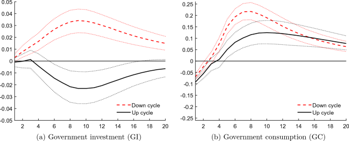
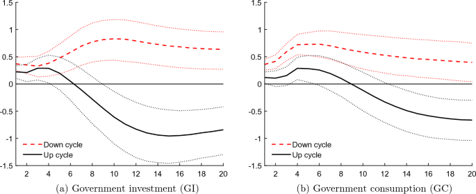
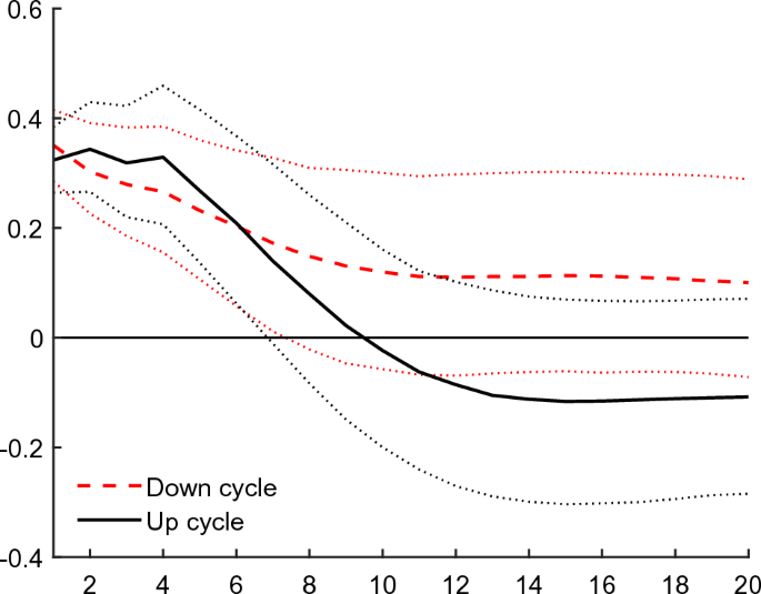
We investigate the impact of the financial cycle on fiscal policy by estimating fiscal multipliers for different types of government spending that are contingent on two states determined by the financial cycle. To obtain our estimates, we extend the threshold VAR method from a single country to a panel of high-income countries. Our results indicate that the multiplier for government investment is affected by the state of the financial cycle: while the initial impact is positive for both states, in an upturn it turns negative, while in a downturn it remains positive. In the case of government consumption, the multiplier does not seem to significantly depend on the financial cycle. However, jointly conditioning on the financial and business cycles produces multipliers of government consumption which vary over the states of both cycles. This contrasts with the results for government investment which are left essentially unchanged by the joint conditioning on the four states defined by both cycles.


Notes
The term “tight” for the credit regime suggests that the mechanism is supply driven, whereas it is also possible that the low level of credit is at least partially due to low demand.
Our code is based on the univariate TVAR estimation program by Gabriel Bruneau, freely available from his homepage.
We experimented with regime-dependent averages, this being the most flexible specification. This did not influence our main results in any noteworthy fashion. Results are available upon request.
Replacing the real interest rate by the nominal rate, to allow for the strict monetary policy reaction, does not alter the results.
Australia, Belgium, Canada, Denmark, Finland, France, Germany, Ireland, Italy, Japan, the Netherlands, Norway, South Korea, Spain, Sweden, Switzerland, UK, USA.
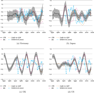
These data are based on the detrended credit-to-GDP gap using the HP-filter with \(\lambda _{\textrm{HP}}= 4\)00,000. We obtained these detrended series from the BIS (Drehmann et al. 2016). The relatively large value of \(\lambda _{\textrm{HP}}\) they use to detrend the credit gap only removes the long-term trend, leaving the longer frequency cycle associated with the financial cycle in their series. This approach, however, also allows the higher frequencies associated with the business cycle to pass through the filter and remain in their financial cycle measure. To obtain a cleaner series containing only the longer financial cycle frequencies, we HP-filter the BIS’s series again with \(\lambda _{\textrm{HP}}=1600\) and use the resulting HP-filter trend component to obtain a smoother financial cycle. In this way we remove the higher business cycle frequencies from the BIS’s series.
The Schüler cycles we received from the authors are smoothed using a six-quarter one-sided moving average based on the weights of a Bartlett window. We demean the Schüler cycles to ensure that they fluctuate around zero, instead of 0.5 as in Schüler et al. (2020). Their approach, the power cohesion method, maps the growth rates of financial variables (such as credit volumes and house prices) into an empirical cumulative distribution function between zero and one. Therefore, these series do not exhibit long-term trends.
The BIS kindly provided us with their financial cycle estimates.
A special thanks to Yves Schüler and colleagues for providing their financial cycle estimates.
For example, in the cast of the BIS estimates, we lose in total 366 observations, which is a little under 10% of our total number of observations.
The phase concordance index is a measure for co-movement between two cycles, say, f and b (see Harding and Pagan 2002). The corresponding expression for country i is given by \(\Phi ^{fb}_{i}=1/T\sum _t\left( \phi ^f_{it}\phi ^b_{it}+(1-\phi ^f_{it})(1-\phi ^b_{it})\right) \), where \(\phi ^{.}_{it}\) is 1 when the cycle is in an upturn and 0 when it is in a downturn as defined in the paper. If the phase concordance index equals 0 both cycles are perfectly counter-cyclical and when it equals 1 both cycles are perfectly pro-cyclical. If two cycles are independent we obtain the expected phase concordance, which can be obtained by replacing \(\phi ^{.}_{it}\) with fraction of time spent in an upturn for both cycles.
We have obtained higher concordance indices of around 0.6 between the Schüler cycle with a lead of two to eight quarters and the CPB cycle measures. A lead of two to eight quarters is actually short compared to the length of the financial cycle and there is still substantial overlap between the up- and down-phases of the Schüler and the CPB cycle.
When necessary we seasonally adjust the data using the X-12 algorithm.
Using other values for \(\lambda _{\textrm{HP}}\) yields qualitatively similar results.
We follow Hamilton (2018), who advises to use \(p=3\) and \(h=8\) for quarterly data.
If we include a short-term nominal interest rate (of the OECD’s Main Economic Indicators) instead of the real rate, all impulse responses are (roughly) unchanged aside from the interest rate. In this case the responses of the nominal rate display a resemblance of a standard Taylor rule for monetary policy with an increase following a rise in inflation, and a reduction after a drop in inflation.
We use the Fisher information matrix to calculate the standard error. However, because the log-likelihood is highly nonlinear, it is not certain that this results in a reliable standard error.
For the endogenous threshold 40% of the observations occur during an upturn of the financial cycle, while in the case of the exogenous threshold this percentage is 48%.
Austria, Germany, Italy, South Korea, The Netherlands, Sweden, and Switzerland show distinctly different patterns from the other countries and the overall main results. Denmark deviates to a lesser extent. For some of these countries, the data cover a shorter time period. However, it is also possible that an insufficient lag length, or a different underlying economic mechanism driving the interaction between the financial cycle and the investment multiplier might explain these results. We leave this for future research.
See footnote 16, replacing the real rate for a nominal rate does not change the results.
Germany, France, Japan, Norway, South Korea, Spain, The Netherlands, Switzerland and the USA show different patterns from the other countries and the overall main results (also see footnote 19).
To save space, the results are available upon request.
The results are also robust for the use of 2 lags, corresponding to 8 lags when using quarterly data. Since the information criteria only support the use of at most 6 lags when using quarterly data, there is no point in adding more lags to the model.
Changing the order of the endogenous variables leads indeed to identical results.
We find the same result with private GDP when using annual data.
Data are obtained from the World Bank over the period 1960–2016. The results are almost identical if we use the openness in 2016 instead of the entire sample.
Open economies: Belgium, Denmark, Ireland, the Netherlands, Norway, Sweden and Switzerland. The remaining eleven countries are closed economies.
Data obtained from Oxford Economics over the period 1980–2018.
Other orderings of the VAR model including debt lead to similar results.
Using the level of debt in 2017 instead of the entire sample, and using a cut-off of 100% such as Corsetti et al. (2012), yields similar results.
Highly indebted countries: Belgium, Canada, Denmark, France, Italy, Japan, the Netherlands and the USA. The remaining ten countries are all lowly indebted countries.
Belgium, Finland, France, Germany, Ireland, Italy, the Netherlands and Spain.
We have also estimated this truncated sample using an endogenous threshold. In this case the results are very similar to our baseline results.
Placing the financial cycle as endogenous variable in a different ordering does not change the results.
Their model also includes seasonal components to correct for any seasonality in the data. We omit this aspect of the model here for simplicity.
Note that the covariance matrices of both disturbance vectors \(\vec \kappa _{it}^{C}\) and \(\vec \kappa _{it}^{C*}\) are restricted to be equal. This restriction is standard, see Harvey (1991) for details.
Asymptotically, however, the two financial cycles will be qualitatively the same, only differing in their amplitude.
References
Abiad A, Furceri D, Topalova P (2016) The macroeconomic effects of public investment: evidence from advanced economies. J Macroecon 50:224–240
Afonso A, Baxa J, Slavík M (2018) Fiscal developments and financial stress: a threshold VAR analysis. Empir Econ 54(2):395–423
Aikman D, Lehnert A, Liang JN, Modugno M (2016) Financial vulnerabilities, macroeconomic dynamics, and monetary policy. In: Finance and economics discussion series 2016-055. Board of Governors of the Federal Reserve System (US)
Alichi A, Shibata I, Tanyeri K(2019) Fiscal policy multipliers in small states. IMF working papers 19/72. International Monetary Fund
Antonakakis N, Breitenlechner M, Scharler J (2015) Business cycle and financial cycle spillovers in the G7 countries. Q Rev Econ Finance 58:154–162
Auerbach AJ, Gorodnichenko Y (2012) Measuring the output responses to fiscal policy. Am Econ J Econ Policy 4(2):1–27
Balke NS (2000) Credit and economic activity: credit regimes and nonlinear propagation of shocks. Rev Econ Stat 82(2):344–349
Batini N, Eyraud L, Forni L, Weber A (2014) Fiscal multipliers: size, determinants, and use in macroeconomic projections. IMF technical notes and manuals 2014/04. International Monetary Fund
Baum A, Poplawski-Ribeiro M, Weber A (2012) Fiscal multipliers and the state of the economy. IMF working papers 12/286. International Monetary Fund
Beetsma R, Giuliodori M, Klaassen F (2008) The effects of public spending shocks on trade balances and budget deficits in the European Union. J Eur Econ Assoc 6(2–3):414–423
Beetsma R, Giuliodori M, Klaassen F (2009) Temporal aggregation and SVAR identification, with an application to fiscal policy. Econ Lett 105(3):253–255
Benetrix A, Lane P (2015) Financial cycles and fiscal cycles. Trinity College Dublin, Dublin, pp 315–346
Blanchard O, Perotti R (2002) An empirical characterization of the dynamic effects of changes in government spending and taxes on output. Q J Econ 117(4):1329–1368
Boehm CE (2020) Government consumption and investment: Does the composition of purchases affect the multiplier? J Monet Econ 115(C):80–93
Borio C (2014) The financial cycle and macroeconomics: What have we learnt? J Bank Finance 45(C):182–198
Borio C, Disyatat P, Juselius M (2017) Rethinking potential output: embedding information about the financial cycle. Oxf Econ Pap 69(3):655–677
Borsi MT (2018) Fiscal multipliers across the credit cycle. J Macroecon 56(C):135–151
Bouakez H, Guillard M, Roulleau-Pasdeloup J (2020) The optimal composition of public spending in a deep recession. J Monet Econ 114(C):334–349
Budina NT, Gracia B, Hu X, Saksonovs S (2015) Recognizing the bias; financial cycles and fiscal policy. IMF working papers 15/246. International Monetary Fund
Caggiano G, Castelnuovo E, Colombo V, Nodari G (2015) Estimating fiscal multipliers: news from a non-linear world. Econ J 125(584):746–776
Caldara D, Kamps C (2017) The analytics of SVARs: a unified framework to measure fiscal multipliers. Rev Econ Stud 84(05):1015–1040
Callegari G, Melina G, Batini N (2012) Successful austerity in the United States, Europe and Japan. IMF working papers 12/190. International Monetary Fund
Canzoneri M, Collard F, Dellas H, Diba B (2016) Fiscal multipliers in recessions. Econ J 126(590):75–108
Carrillo J, Poilly C (2013) How do financial frictions affect the spending multiplier during a liquidity trap? Rev Econ Dyn 16(2):296–311
Cerutti E, Claessens S, Rose AK (2019) How important is the global financial cycle? Evidence from capital flows. IMF Econ Rev 67(1):24–60
Christiano LJ, Eichenbaum M, Evans CL (1999) Monetary policy shocks: What have we learned and to what end? In: Taylor JB, Woodford M (eds) Handbook of macroeconomics, vol 1. Elsevier, Amsterdam, pp 65–148
Christiano L, Eichenbaum M, Rebelo S (2011) When is the government spending multiplier large? J Polit Econ 119(1):78–121
Claessens S, Kose MA, Terrones ME (2012) How do business and financial cycles interact? J Int Econ 87(1):178–190
Coenen G, Straub R, Trabandt M (2012) Fiscal policy and the great recession in the Euro area. Am Econ Rev 102(3):71–76
Corsetti G, Meier A, Müller GJ (2012) What determines government spending multipliers? Econ Policy 27(72):521–565
Danthine J-P (2012) Taming the financial cycle. Swiss National Bank, Speech at SUERF Colloquium 2012, Zurich
Dosi G, Fagiolo G, Napoletano M, Roventini A (2013) Income distribution, credit and fiscal policies in an agent-based Keynesian model. J Econ Dyn Control 37(8):1598–1625
Drehmann M, Borio C, Tsatsaronis K (2012) Characterising the financial cycle: Don’t lose sight of the medium term! BIS working papers 380. Bank for International Settlements
Drehmann M, Pradhan K, Wooldridge P, Santos M, Vidal J, Szemere R (2016) Recent enhancements to the BIS statistics. BIS Q Rev, pp 35–44
Ellahie A, Ricco G (2017) Government purchases reloaded: informational insufficiency and heterogeneity in fiscal VARs. J Monet Econ 90:13–27
Fernández-Villaverde J (2010) Fiscal policy in a model with financial frictions. Am Econ Rev 100(2):35–40
Ferraresi T, Roventini A, Fagiolo G (2015) Fiscal policies and credit regimes: a TVAR approach. J Appl Econom 30(7):1047–1072
Gechert S, Mentges R (2018) Financial cycles and fiscal multipliers. Appl Econ 50(24):2635–2651
Gechert S, Rannenberg A (2018) Which fiscal multipliers are regime-dependent? A meta-regression analysis. J Econ Surv 32(4):1160–1182
Gieve SJ (2008) The financial cycle and the UK economy. Speech at London Stock Exchange. Bank of England, London, p 2008
Gonzalez-Garcia JR, Lemus A, Mrkaic M (2013) Fiscal multipliers in the ECCU. IMF working papers 13/117. International Monetary Fund
Hamilton JD (2018) Why you should never use the Hodrick–Prescott filter. Rev Econ Stat 100(5):831–843
Hansen BE (1996) Inference when a nuisance parameter is not identified under the null hypothesis. Econometrica 64(2):413–430
Hansen BE (1997) Inference in TAR models. Stud Nonlinear Dyn Econom 2(1):1–16
Harding D, Pagan A (2002) Dissecting the cycle: a methodological investigation. J Monet Econ 49(2):365–381
Harvey AC (1991) Forecasting, structural time series models and the Kalman filter. Cambridge Books, no. 9780521405737. Cambridge University Press
Hebous S (2011) The effects of discretionary fiscal policy on macroeconomic aggregates: a reappraisal. J Econ Surv 25(4):674–707
Holmström B, Tirole J (1998) Private and public supply of liquidity. J Polit Econ 106(1):1–40
Huidrom R, Kose MA, Lim JJ, Ohnsorge FL (2020) Why do fiscal multipliers depend on fiscal positions? J Monet Econ 114(C):109–125
Ilzetzki E, Mendoza EG, Végh CA (2013) How big (small?) are fiscal multipliers? J Monet Econ 60(2):239–254
Jordà Ò, Taylor AM (2016) The time for austerity: estimating the average treatment effect of fiscal policy. Econ J 126(590):219–255
Jordà Ò, Schularick M, Taylor AM, Ward F (2019) Global financial cycles and risk premiums. IMF Econ Rev 67(1):109–150
Kamps C (2005) The dynamic effects of public capital: VAR evidence for 22 OECD countries. Int Tax Public Finance 12(4):533–558
Laeven L, Valencia F (2018) Systemic banking crises revisited. IMF working paper, 206, pp 1–47
Leeper EM, Walker TB, Yang S-CS (2010) Government investment and fiscal stimulus. J Monet Econ 57(8):1000–1012
Leeper EM, Traum N, Walker TB (2017) Clearing up the fiscal multiplier morass. Am Econ Rev 107(8):2409–2454
Luginbuhl R (2020) Estimation of the financial cycle with a rank-reduced multivariate state-space model. CPB discussion paper. CPB Netherlands Bureau for Economic Policy Analysis
Luginbuhl R, Soederhuizen B, Teulings R (2019) Estimates of the financial cycle for advanced economies. CPB discussion paper. CPB Netherlands Bureau for Economic Policy Analysis
Maddala DS (1977) Econometrics. McGraw-Hill, New York
Mumtaz H, Sunder-Plassmann L (2021) Nonlinear effects of government spending shocks in the USA: evidence from state-level data. J Appl Econom 36(1):86–97
Mumtaz H, Pirzada A, Theodoridis K (2018) Non-linear effects of oil shocks on stock prices. Working papers 865. Queen Mary University of London, School of Economics and Finance
Pereira AM (2000) Is all public capital created equal? Rev Econ Stat 82(3):513–518
Pesaran M, Smith R (1995) Estimating long-run relationships from dynamic heterogeneous panels. J Econom 68(1):79–113
Praet P (2016) Financial cycles and monetary policy. ECB, Speech in the Context of a Panel on International Monetary Policy, Beijing
Ramey VA (2011a) Can government purchases stimulate the economy? J Econ Lit 49(3):673–685
Ramey VA (2011b) Identifying government spending shocks: it’s all in the timing. Q J Econ 126(1):1–50
Ramey VA (2019) Ten years after the financial crisis: What have we learned from the renaissance in fiscal research? J Econ Perspect 33(2):89–114
Ramey VA, Shapiro MD (1998) Costly capital reallocation and the effects of government spending. In: Carnegie-Rochester conference series on public policy, vol 48. Elsevier, pp 145–194
Ramey VA, Zubairy S (2018) Government spending multipliers in good times and in bad: evidence from US historical data. J Polit Econ 126(2):850–901
Romer CD, Romer DH (2010) The macroeconomic effects of tax changes: estimates based on a new measure of fiscal shocks. Am Econ Rev 100(3):763–801
Rozite K, Bezemer DJ, Jacobs JPAM (2019) Towards a financial cycle for the US, 1973–2014. N Am J Econ Finance 50:101023
Rünstler G, Vlekke M (2018) Business, housing, and credit cycles. J Appl Econom 33(2):212–226
Schüler YS, Hiebert PP, Peltonen TA (2020) Financial cycles: characterisation and real-time measurement. J Int Money Finance 100:102082
Strohsal T, Proaño CR, Wolters J (2019) Characterizing the financial cycle: evidence from a frequency domain analysis. J Bank Finance 106:568–591
Traum N, Yang S-CS (2015) When does government debt crowd out investment? J Appl Econom 30(1):24–45
Tsay RS (1998) Testing and modeling multivariate threshold models. J Am Stat Assoc 93(443):1188–1202
Winter J, Koopman SJ, Hindrayanto I, Chouhan A (2017) Modeling the business and financial cycle in a multivariate structural time series model. DNB Working Papers 573. Netherlands Central Bank, Research Department
Woodford M (1990) Public debt as private liquidity. Am Econ Rev 80(2):382–388
Funding
This research did not receive any grant from funding agencies in the public, commercial, or not-for-profit sectors.
Author information
Authors and Affiliations
Corresponding author
Ethics declarations
Conflict of interest
The authors have no competing interests to declare that are relevant to the content of this article.
Ethical approval
This article does not contain any studies with human participants or animals performed by any of the authors.
Additional information
Publisher's Note
Springer Nature remains neutral with regard to jurisdictional claims in published maps and institutional affiliations.
We would like to thank Roel Beetsma, Adam Elbourne, Albert van der Horst, Clemens Kool, Bert Smid, seminar participants and the anonymous referees for their valuable comments that helped improve this paper.
Appendices
A State space model of CPB financial cycle
We denote the credit data for country i by \(y^1_{it}\) and the housing price index by \(y^2_{it}\) and define the data column vector \(\vec {y}_{it}=\left( y^1_{it}, y^2_{it}\right) '\). Similarly, we denote the vector of the financial cycles for credit and the housing price index of country i as \(\vec {f}_{it}\). We use the same notion for the vector of the business cycle components, \(\vec {b}_{it}\). The state space model also includes two local linear trend components, one for credit and one for the housing price index, giving rise to the vector \(\vec {\mu }_{it}\) to capture the growth dynamics in the data. Each trend component is itself affected by a random walk growth component, which for both series we also denote by a vector: \(\vec {\beta }_{it}\). Using this notation we can express the model in Luginbuhl et al. (2019) as followsFootnote 35:
where the financial cycle component is given by
and the business cycle component by
Note that the components \(\vec {b}_{it}^{*}\) and \(\vec {f}_{it}^{*}\) are only required for the construction of the cycle components \(\vec {b}_{it}\) and \(\vec {f}_{it}\). Also note that the model contains the vector disturbance terms \(\vec \varepsilon _{it}\), \(\vec \eta _{it}\), \(\vec \zeta _{it}\), as well as \(\vec \kappa _{it}^C \sim N\left( 0, \Omega _{\kappa ,i}^C \right) \) and \(\vec \kappa _{it}^{C*} \sim N\left( 0, \Omega _{\kappa ,i}^C \right) \) for \(C=b\) or f.Footnote 36
The state space model (Luginbuhl et al. 2019) use in the estimation of the financial cycle is closely related to work of Rünstler and Vlekke (2018) and Winter et al. (2017), which are also based on unobserved cycle components to model financial cycles. The main difference here being that the estimation method by Luginbuhl et al. (2019) imposes the restriction of there being only one shared stochastic process driving both financial cycle components in their bi-variate model. This restriction is necessary to help identify one financial cycle for each country. In fact the financial cycle estimate \(f_{it}\) is the cycle component for the credit data. Although the housing price index shares the same stochastic disturbance driving the cycle, the housing price index has its own starting value. As a result, the housing price index financial cycle can deviate from the credit cycle in the initial part of the sample period.Footnote 37
The bi-variate state space models distinguish between the business cycle and the financial cycle by assuming that the financial cycle has a longer period cycle than the business cycle. The financial cycles are full-information, Kalman smoothing estimates obtained using Bayesian Markov Chain Monte Carlo or MCMC methods.
B Data series
C Correlation and phase concordance between financial and business cycles
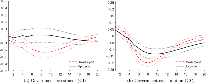
D IRFs of inflation and real interest rate, baseline specification
E Baseline results in alternative specifications
1.1 E.1 Figures for baseline results in alternative specifications
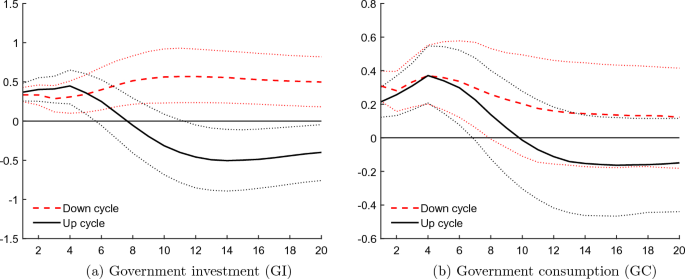
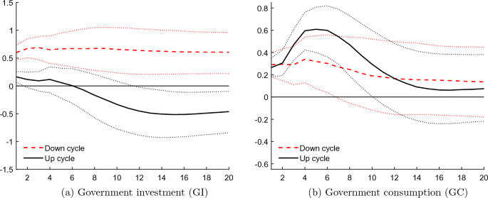
Cumulative fiscal multipliers with an endogenous threshold. See the note in Fig. 2 for more information
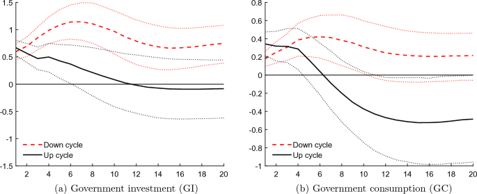
Cumulative fiscal multipliers using weighted mean group estimation. We only use 2 lags instead of 4 because of a shortage of degrees of freedom at the country level. We weight the country-specific cumulative fiscal multipliers using number of observations per country as weight and take the average to construct the weighted mean group estimate. See the note in Fig. 2 for more information
1.2 E.2 Alternative financial cycles
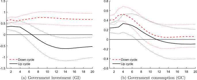
Cumulative fiscal multipliers using the BIS cycle as financial cycle. See the note in Fig. 2 for more information
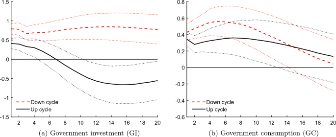
Cumulative fiscal multipliers using credit-to-GDP gap as financial cycle. See the note in Fig. 2 for more information
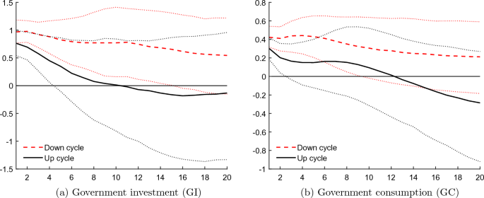
Cumulative fiscal multipliers using the Schüler financial cycles. See the note in Fig. 2 for more information
F Additional figures of the robustness checks
See Figs. 13, 14, 15, 16 and 17.
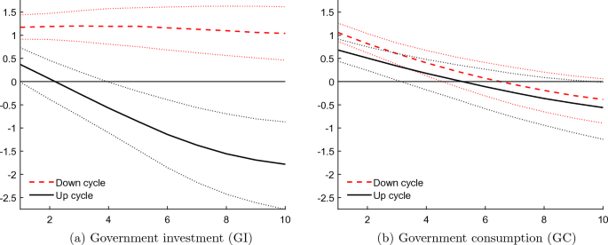
Cumulative fiscal multipliers with yearly data. The model is estimated with year data and include \(L=1\) lags. See the note in Fig. 2 for more information
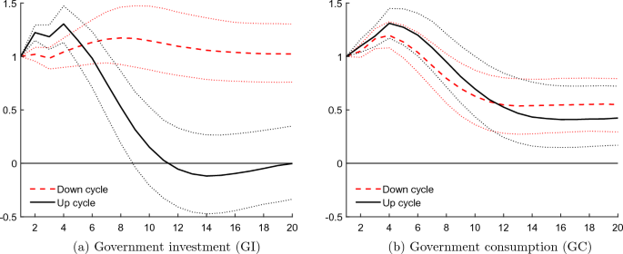
Cumulative fiscal multipliers with private GDP as first endogenous variable. Private GDP is ordered as the first endogenous variable. Therefore, the cumulative multipliers are equal to one by construction in the first period. See the note in Fig. 2 for more information
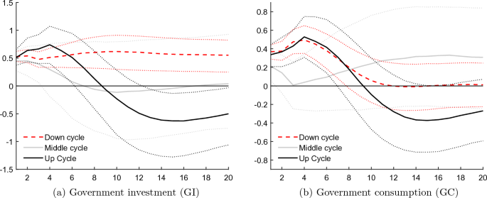
Cumulative fiscal multipliers with three regimes and two endogenous thresholds. See the note in Fig. 2 for more information
Cumulative fiscal multipliers for total government expenditure. See the note in Fig. 2 for more information
Rights and permissions
Springer Nature or its licensor (e.g. a society or other partner) holds exclusive rights to this article under a publishing agreement with the author(s) or other rightsholder(s); author self-archiving of the accepted manuscript version of this article is solely governed by the terms of such publishing agreement and applicable law.
About this article
Cite this article
Soederhuizen, B., Teulings, R. & Luginbuhl, R. Estimating the impact of the financial cycle on fiscal policy. Empir Econ 65, 2669–2709 (2023). https://doi.org/10.1007/s00181-023-02448-0
Received:
Accepted:
Published:
Issue Date:
DOI: https://doi.org/10.1007/s00181-023-02448-0


