
Abstract
The paper presents a new multi-material topology optimization method with a novel adjoint sensitivity analysis that can accommodate not only multiple plasticity but also multiple hardening models for individual materials in composite structures. Based on the proposed method, an integrated framework is developed which details the nonlinear finite element analysis, sensitivity analysis and optimization procedure. The proposed method and framework are implemented and illustrated by three numerical examples presented in this paper. An in-depth analysis of the numerical results has revealed the significant impact of the selection of plasticity and hardening model on the results of topology.
1 Introduction
Due to the increasingly high demand for lightweight materials with specific mechanical characteristics in various fields, such as structural engineering and aerospace, composite structures have drawn wide attention from both the research and design community. Composite designs are highly diverse, and the composite materials can be easily placed into free-form combinations, to achieve specific and more desirable designs. These designs exhibit increased strength, toughness, erosion resistance and antifatigue properties compared to single materials. A two-phase composite, where one material, acting as a reinforcing element, is embedded into another material matrix in the form of strips, sheets, or grids, is becoming more attractive for many practical applications. The material for these phases can be steel, aluminium, polymer, wood, concrete, etc., and there is a need to distribute these materials efficiently to maximize the contribution of each material.
The topology optimization technique is an effective tool, especially with complex boundary and loading conditions, that has been used by researchers to design a conceptual structural layout. Extensive research has been conducted on the implementation of topology optimization on single materials with linear elastic properties (Guan 2005; Bruggi 2009; Bruggi 2010). The resulting truss-like topology can be regarded as a strut-and-tie model based on the compression and tension regions. Multiphase linear elastic material optimization has also been developed by interpolating the lower bound of the design variable to a second material candidate (Bendsøe and Sigmund 1999; Huang and Xie 2009). However, linear-elastic material modelling is inadequate when the structural behaviour of the realistic real-life design exceeds the elastic range. Studies emerged to address the problem, especially for those materials such as concrete or soil that have unequal compression and tensile strength incorporating the different mechanical properties of composite materials into topology optimization (Querin et al. 2010; Victoria et al. 2011; Liu and Qiao 2011; Luo and Kang 2012; Luo et al. 2015). In recent decades, the nonlinear material behaviour has also been considered to achieve a more reliable design by topology optimization. Initial studies considering topology optimization with material nonlinearity focus on a single material problem (Yuge and Kikuchi 1995; Maute et al. 1998; Schwarz et al. 2001; Yoon and Kim 2007). In the most recent research, Wallin et al. (Wallin et al. 2016) succeeded in combining finite strain isotropic hardening plasticity with topology optimization. Zhang and Lei (Zhang et al. 2017) went further and accounted for plastic anisotropy in conjunction with topology optimization. The BESO optimization method, considering the von Mises isotropic hardening plasticity, is also applied in layout design in (Xia et al. 2017). Li et al. (Li et al. 2017) proposed a topology optimization procedure incorporating with the von Mises criteria employing various hardening rules to maximize the energy dissipation under cyclic loading.
In two-phase elastoplastic material optimization, the obtained topology significantly depends on the loading whether it is elastic or plastic dominated (Kato et al. 2015). However, there are few studies considering material nonlinearity for a multiphase optimization problem. For example, Swan and Kosaka (Swan and Kosaka 1997) presented a framework of continuous structural topology optimization for elastoplastic applications based on the Voigt and Reuss mixing formulation. An approach presented in Bogomolny and Amir’s (Bogomolny and Amir 2012) work applied the topology optimization method in a concrete and steel layout design taking into account both the yield criteria and the post yielding performance. Nakshatrala and Tortorelli (Nakshatrala and Tortorelli 2015) proposed a framework to distribute the two elastoplastic material phases to optimize energy dissipation under impact loading. Kato et al. (Kato et al. 2015) developed an analytical sensitivity approach for topology optimization in nonlinear composites.
The von Mises plastic material model is adopted in most of the aforementioned studies, and they all employ the isotropic hardening rule, where the radius of the yield surface increases based on the accumulated effective plastic strain. However, kinematic hardening, where the radius remains constant but the centre of the subsequent yield surface is moved by shift stress, is often overlooked, despite many practical materials such as polycrystalline metals, exhibiting combined properties of isotropic and kinematic hardening. In addition, except for the commonly used yielding criterion of von Mises that is widely applied to model metal materials, the Drucker-Prager yield criterion is usually used to describe pressure-dependent materials such as concrete or soil (Luo and Kang 2012; Bogomolny and Amir 2012; Li and Zhang 2018).
There is an increasing demand for the topology optimization technique to efficiently distribute material phases for composite structures. Therefore, it is necessary to consider more types of hardening rules, following multiple yield criteria, and incorporate the topology optimization method to achieve a more realistic and reliable design.
This study proposes a topology optimization procedure for a multiphase material distribution problem. Here, the material candidates are associated with kinematic hardening or mixed isotropic and kinematic hardening with the flexibility of combining different plasticity models. Moreover, the proposed framework also offers the flexibility of assigning different hardening rules to each single material phase by using the design variables to interpolate the permissible yielding stress surface into the topology optimization. For example, the von Mises or the Drucker-Prager plasticity model is applied to both phases, but one follows the isotropic hardening rule while kinematic hardening is assigned to the other. To illustrate the advantage of the proposed framework and method, three design examples are tested, and the results are presented in this paper. In the first two examples, several material models were created including (1) the von Mises and the Drucker-Prager yield criterion applied to each phase, respectively; (2) the von Mises yield criterion applied to both phases; and (3) the Drucker-Prager yield criterion applied to both phases. All cases in model (1) employ the kinematic hardening, while in model (2), they employ the combined isotropic/kinematic hardening rule, which enables the investigation into the influence of the plasticity model on the resulting topology. In the third example, several material models using the same plasticity model are employed for the composite structure but following various hardening rules. Isotropic, kinematic, or mixed isotropic and kinematic hardening was performed to study whether the post-yielding behaviour would affect the optimization results of multiphase material distribution.
This work successfully achieved the above objective of incorporating structural analysis with specific multiphase plasticity into topology optimization. The residual equilibriums on an integration point level are defined based on various plastic material modelling. The corresponding path-dependent sensitivity analysis expression is derived in this paper, by using a path-dependent adjoint method that followed the framework described by Michaleris et al. (Michaleris et al. 1994). The method of moving asymptotes (MMA) (Svanberg 1987) was applied to update design variables. Through a comparative analysis, this study highlights the importance of considering material properties with precision for multiphase optimization design.
2 Elastoplastic material with strain hardening model
2.1 Yielding criterion
The behaviour of some material is initially elastic and becomes plastic with the existence of the irreversible strain when the applied force exceeds the elastic limit, which is known as elastoplasticity. In this study, two types of yielding criterion are considered to describe the material elastoplasticity. The von Mises yielding criterion is widely used to predict the yielding of metals that have equal strength in compression and tension. In contrast, for those pressure-dependent materials, e.g. rock or soil, the Drucker-Prager yielding criterion is generally employed to consider the hydrostatic pressure. It is obtained by adding a mean stress term on the von Mises yielding based formulation as
where the material constant α is equal to zero when it corresponds to the von Mises yield function and k represents the permissible yielding stress surface, which will be discussed in the next subsection. The first invariant of the stress tensor I1 and the second invariant of the deviatoric stress tensor J2 are written as
and
2.2 Strain hardening model
When the plastic loading progresses, the yield stress may increase rather than remain constant according to the plastic deformation, which is called strain hardening. For some applications, the ideal assumption of material with elastic perfectly plasticity may not be adequate to simulate the problem; therefore, the strain hardening is essential to be considered in a two-material topology optimization. Here, three types of hardening models are applied: isotropic, kinematic and combined isotropic/kinematic hardening. In the isotropic hardening model, the yield surface with a fixed central location grows uniformly according to the effective plastic strain. However, the kinematic hardening rule enables the elastic domain stays constant while the subsequent yield surface moves following the strain hardening. Moreover, some materials are generally described by a combination of these two models as follows:
where σY denotes the initial yield stress, ep is the effective plastic strain and the plastic modulus Hp is a constant, as all hardening rules are assumed to be linear in this paper. ϕ is a parameter representing the combined effect for a combined isotropic/kinematic hardening model. For the isotropic hardening, ϕ equals 0, and for the kinematic hardening, ϕ equals 1.
2.3 Elastoplasticity model
According to the assumption in the small deformation elastoplasticity, the rate of the total strain \( \dot{\upvarepsilon} \) can be decomposed into the rate of the elastic strain \( {\dot{\upvarepsilon}}^{\mathrm{e}} \) and the plastic strain \( {\dot{\upvarepsilon}}^{\mathrm{p}} \) as
The elastic strain relates to the stress by using the fourth-order constitutive tensor D. And the plastic strain evolves in the direction normal to the flow potential that is associated to the yield function f in this study, which is given by
where γ is the non-negative plastic consistency parameter. It is governed by the Kuhn-Tucker conditions, i.e.
3 Nonlinear finite element analysis
The global equilibrium for the complete structure should be satisfied in the finite element analysis, which can be expressed as
with
where Rn represents the residual on the global level in loading step n, which is equal to the difference between the external applied force \( {\mathrm{R}}_{ext}^n \) and the internal force \( {\mathrm{R}}_{int}^n \)in the same step. B is the strain-displacement matrix.fB, fs and P denote the internal body force, surface traction and the external concentrated load, respectively. Also, the local residuals on each integration point are constructed and required to be sufficiently small throughout the analysis. In this study, a four-node quadrilateral plane stress element with four integration points is utilized for all examples. Thus, the expression of residual H on the loading increment n for a full structure is formed by embedding the local residuals on each integration point of each element into a global matrix:
where e is the number of elements, i represents the number of integration points, and j corresponds to the number of local residuals required on an integration point level based on the specified plasticity model and hardening rule. In the elastic incremental stage, for the material candidate modelled with either the von Mises or the Drucker-Prager yielding criterion, the local residuals \( {\mathrm{H}}_{eij}^n \) are defined in the same formulations as
Here the above residual describes the condition when the elastoplastic material model follows the kinematic or combined hardening rule, where Ue is the elemental nodal displacement vector; σei, aei and epei represent the stress, back stress and the equivalent plastic strain obtained on each integration point, respectively.
However, in the plastic stage, the local residuals for both materials using the von Mises model with kinematic or combined hardening rule are given by
where η is the shifted stress deviator defined as the difference between the stress deviator s and the back stress deviator a, i.e. η = s − a.
When one of the material phases is modelled by the Drucker-Prager yield criterion and accompanied with the isotropic hardening, the corresponding local residuals become
where the material constant αe and the hardening combined effect parameter ϕe corresponding to a specified element e are related to the density design variables. Also, due to the nature of the Drucker-Prager model where the hydrostatic pressure is considered, the direction of the plastic strain normal to the flow potential is described as
while in the previous case presented in (12), based on the von Mises yield criterion, the yield function is defined in a deviatoric space only as the volumetric stress is independent of plastic deformation. Thus, the plastic strain evolves in the direction:
In the case where isotropic hardening is applied to both materials, the centre of the yielding surface is fixed on a certain point means that the back stress a does not exist so as the related residual equation in both elastic and plastic stage is eliminated. Correspondingly, only three variables on each integration point are considered, i.e. \( {\mathrm{v}}^n=\left[{\boldsymbol{\sigma}}_{ei}^n\kern0.5em {e}_{pei}^n\kern0.5em \Delta {\gamma}_{ei}^n\right] \). However, in the kinematic/combined hardening model, the yielding surface moves following the plastic deformation; therefore, the required variables would be defined as \( {\mathrm{v}}^n=\left[{\boldsymbol{\sigma}}_{ei}^n\kern0.5em {\mathrm{a}}_{ei}^n\kern0.5em {e}_{pei}^n\kern0.5em \Delta {\gamma}_{ei}^n\right] \).
4 Topology optimization
4.1 Problem statement
For the linear elastic material topology optimization, minimizing the mean compliance is often used as the objective function. While for elastoplastic materials, minimizing the end compliance or maximizing the total plastic energy is commonly used as the objective function in topology optimization. In this paper, the displacement loading method is applied throughout the nonlinear analysis due to its relative stability. And the end compliance–related objective function is achieved by maximizing the final equivalent external load corresponding to the prescribed displacement. Also, based on the consideration of the material nonlinearity, the optimization statement should be coupled with the global equilibrium and the local residual conditions that satisfied at each step as shown below:
where xe depicts the elemental design variable updated in each iteration and V∗ is the prescribed target volume fraction of the design domain. Pref is a constant external load vector in which each element corresponding to a degree of freedom. When there is a prescribed displacement applied on a degree of freedom, the corresponding element equals to 1 otherwise will be 0. φN denotes the load factor at the final loading step calculated from the global equilibrium, and it is a scalar. The objective function stated in (16) is only valid under certain load conditions and will lead to a complicated sensitivity analysis. Thus, Amir et al. (Bogomolny and Amir 2012) proposed a simplified hybrid approach using the load-controlled concept to generate a more applicable objective function as follows:c(x) = PNuN, but the actual nonlinear analysis is performed through a displacement-controlled method.
4.2 Material interpolation
In this paper, the elastoplastic behaviour of a two-material-phase problem will be interpolated into topology optimization by utilizing the design variable. The elastic constitutive tensor can be written as
with
where l is the second-order unit tensor and I is the symmetric fourth-order unit tensor. v is the Poisson’s ratio, and from the relationship presented above, it can be observed that the Lame’s constants λ and μ are proportional to Young’s modulus E. The following shows the interpolating functions:
Particularly, when different plasticity model and hardening rules are adopted by each material phase, e.g. the von Mises model with kinematic hardening is applied to the first material, and the second material employs the Drucker-Prager model with isotropic hardening, two more interpolation functions need to be considered as
where the penalisation value \( {p}^{\lambda }={p}^{\mu }={p}^{\sigma_Y}={p}^{H_p}={p}^{\alpha }={p}^{\phi }=3 \) is assumed throughout this study. A lower penalty number may lack effectiveness to distinguish intermediate densities to black and white, while if it is too high, the model would risk unfavourable instability induced by nonlinearity. Therefore, a penalty number equal to 3 is widely used in many literatures (Bendsøe and Sigmund 1999; Huang and Xie 2009; Luo and Kang 2012; Luo et al. 2015). Equation (20) is one of the important interpolations proposed in this paper which develops a straightforward approach for adopting different plasticity models and hardening rules for each material phase. This is the pivoting interpolation that later articulated with (36–37), a key step to convert conventional adjoint sensitivity analysis for the single material phase to dual-material phase analysis. In particular, a specific yielding criterion or strain hardening model can be derived as a special case of (20), i.e. when xe = 1 yields a material phase with von Mises yielding criterion (αe = αmin = 0) and kinematic hardening (ϕe = ϕmax = 1). More details are given in Tables 1, 2 and 3 of the examples in Section 6.
5 Sensitivity analysis
5.1 Adjoint sensitivity analysis
The path-dependent adjoint method is applied to compute the sensitivity of the objective with respect to the design variables. The augmented objective function can be built by adding the global and the local residuals that are infinitely approaching to zero. Also, the objective function c and the global residual R only depend on the nodal displacement u and the variable v, respectively:
where ξn and θn are the adjoint vectors calculated during the sensitivity analysis. The differentiation of the objective function c is equivalent to the derivative of the augmented function \( \hat{c} \) with respect to design variables, and it can be decomposed into an explicit term and an implicit term
In order to eliminate the unknown term of derivatives \( \frac{\partial {\mathrm{u}}^n}{\mathrm{\partial x}} \) and \( \frac{\partial {\mathrm{v}}^n}{\mathrm{\partial x}} \), the backward incremental calculation approach is applied to obtain the Lagrange multipliers θn and ξn for all increments n = 1, …, N:
For the final step N
For steps from n = 1 to N − 1
Therefore, based on the obtained adjoint vector and the derivative of the explicit term, the design sensitivity with respect to the design variables can be written as follows:
Furthermore, the derivatives \( \frac{\partial c}{\partial {\mathrm{u}}^N} \), \( \frac{\partial {\mathrm{H}}^n}{\partial {\mathrm{u}}^n} \), \( \frac{\partial {\mathrm{H}}^{n+1}}{\partial {\mathrm{u}}^n} \), \( \frac{\partial {\mathrm{H}}^n}{\partial {\mathrm{v}}^n} \), \( \frac{\partial {\mathrm{H}}^{n+1}}{\partial {\mathrm{v}}^n} \) and \( \frac{\partial {\mathrm{R}}^n}{\partial {\mathrm{v}}^n} \) are required to solve the above equilibriums presented in (24) and (25). This will be discussed in the next subsection.
5.2 Derivative calculation
When the elastoplastic material employing kinematic or combined hardening rule, the variables vn on integration-point level consist of stresses σn, back stress an, equivalent plastic strain \( {e}_p^n \), and the plastic multiplier Δγn, whereas the back stress an is neglected when the isotropic hardening is applied. Corresponding to the material with elastoplastic kinematic or combined hardening, the required derivatives in matrix form are given as follows:
When the material response stays in the elastic stage
In the plastic stage, for both materials modelled with von Mises yield criterion, the derivatives of the local residual with respect to the variable v and the design variable x can be derived as follows:
with
where \( {\mathrm{I}}_{dev}=\mathrm{I}-\frac{1}{3}1\otimes 1 \) is the fourth-order unit deviatoric tensor. However, for the material phases associated with different plasticity models coupled with various hardening rules, the corresponding derivatives become
Since the volumetric parts of stress (first invariant of stress tensor) I1 are a first-order differential equation in terms of σ, the following expression \( \frac{\partial f}{\partial \boldsymbol{\sigma} \partial \boldsymbol{\sigma}} \) and \( \frac{\partial f}{\partial \boldsymbol{\sigma} \mathrm{\partial a}} \) are equivalent to \( \frac{\partial f}{\partial \boldsymbol{\eta} \partial \boldsymbol{\sigma}} \) and \( \frac{\partial f}{\partial \boldsymbol{\eta} \mathrm{\partial a}} \) as stated in (35). Opposite to the derivatives of Hn with respect to the internal variable vn and the design variable x that are different for materials incorporating with various yielding function in the elastic and plastic step, the following derivatives do not depend on the finite element analysis response:
Therefore, the matrix of the differentiation of Hn need to be adjusted according to the trial elastic condition, which keeps consistency with the analysis at each increment. Also, for the yield criterion incorporating with isotropic hardening, the derivatives of the global residual Rn and the local residual Hn are matrices of smaller size due to the elimination of one variable (back stress an).
6 Examples
Three numerical examples, a simply supported beam, a cantilever beam with a circular opening and an L-shaped bracket, are examined to evaluate the impacts of different yielding criterion and hardening rules on the resulting topologies through the proposed optimization framework for structure with two elastoplastic material phases. All examples are assumed to be in plane stress condition. The optimization procedure is either stopped by the limiting convergence tolerance (10−4in our case) or a stable topology achieved after an adequate number of iterations (300 to 500 in our case).
To accelerate the speed to obtain a stable topology with a clear boundary between the two materials, a step-contract filtering scheme is adopted. By gradually reducing the filter radius during the optimization procedure, a distinct layout can be achieved within 300–500 iterations, with no significant change in topology after these adequate number of iterations. A typical setup of such a filter scheme was designed as follows: filter radii are equal to 5 mm, 2 mm and 1.2 mm when the iterations are between 0 and 150, 150 and 200 and 200 and 300/500, respectively. When a gradual refinement is used, the optimization benefits from obtaining a distinct layout as well as saving computational cost by quickly escaping from the emergence of ‘grey’ areas.
The termination conditions are empirical conditions based on the try-and-error numerical trials. A filtering scheme using a step-contract filter radius was employed to accelerate the topological concentration process during the optimization procedure.
6.1 Simply supported beam
A simply supported beam, length-to-height ratio equals to 4, is shown in Fig. 1. A downward distributed prescribed displacement is applied to the central portion of the top edge. The whole design domain is discretized into 3600 (120 × 30) elements. And the desired volume fraction to the whole design domain is 30%. The prescribed displacement load of U ∗ = 0.5 mm is assumed throughout this example to achieve a plastic design.

Design domain of the simply supported beam
In this example, each material phase has the flexibility of adopting different elastic and plastic material model accompany with various hardening rules. The cases examined in this example include (1) both material with elastic model; (2) both material phases with the von Mises plasticity model and the kinematic hardening; (3) both material phases with the Drucker-Prager plasticity model and the kinematic hardening; and (4) one material phase with the von Mises plasticity model while the other with the Drucker-Prager plasticity model and the post-yielding behaviour of both follow the kinematic hardening, as detailed in Table 1.
The purpose of this example is to investigate the influence of the plasticity model on the results of the optimization design. The mechanical properties of the two material candidates are detailed as follows:
Poisson’s ratio v = 0.3 is adopted for both material candidates. If the Drucker-Prager model is adopted, the material parameter α is required and assumed to be equal to 0.8 in this example. The material models are derived from steel and concrete with reasonable simplification and enable the following numerical simulations. To maintain comparability, the values of the material properties remain constant for all cases.
The resulting distribution of two material phases is shown in black and green in Fig. 2. The first material is presented in black while the second material is presented in green. One can notice that the resulting topology of cases C and D is very similar. This is because material 1 has much higher-yielding strength than material 2. Material 2 may enter the plastic stage much earlier than material 1. When under a relatively small loading/deflection, material 1 may still well be in the post-elastic/early plastic stage, while material 2 has entered the full plastic stage. If different yielding criteria were used for material 1, but the same yielding criterion for material 2, they will not have a significant impact on the resulting topology. Using the resulting topology as the final design, the contour plots of the second principal stress for cases A–D are shown in Fig. 3, which is able to highlight the microstructure of the final design. For clarity, only the stresses of material 2 are plotted, and that of material 1 is plotted as void.

Optimized layouts of cases A–D. a Case A, b Case B, c Case C, d Case D

The corresponding contour plots of the second principal stress for cases A–D. a Case A, b Case B, c Case C, d Case D
Several important findings are summarized below:
-
1)
Adopting different plasticity models for material 2 results in different final topologies. When von Mises plasticity model is used, the mechanical properties are symmetrical in tension and compression, and both of them are much weaker than phase material 1. This leads to an arch shape of topology as shown in Fig. 6(b) in which the structural skeleton, no matter in compression (the arch) and tension (the tie), is all made of material 1 as material 2 is not able to take the loading. As shown in Fig. 3 (b), it is noticeable that around the top-middle area of the beam where the prescribed loading is applied, there is a chuck of material 1 allocated due to the high compressive stress concentration in this area.
In cases C and D, while using Drucker-Prager plasticity model for the second material, empowered with the ability of modelling the relatively higher compressive and lower tensile yielding strength, different resulting topologies are obtained as shown in Fig. 2(c) and (d). In comparison with Fig. 2 (b), there are two main differences that can be observed from the contour plots, (i) some parts of the structural members, as shown in Fig. 4(a), filled with material 1 suffering from compression are replaced by a block of material 2, as shown in Fig. 4(b–c), acting as struts; (ii) the resulting topologies developed in different cases demonstrate different ways to address the compressive stress concentration around the loading area. A pad-shaped structure as shown in Fig. 5(a) is formed by stiff material 1 supported by soft material 2 under. While in Fig. 5(c) and (d), showing the results of cases C and D, respectively, material 2 is modelled with the Drucker-Prager yielding criterion, which allows material 2 to sustain a much higher compression, a pile-shape structure is evolved taking the advantage of the end support underpinned by the Drucker-Prager model.

Comparison of the arch components of case B to cases C and D. a Case B, b Case C, c Case D

Comparison of the punching stiffeners of case B to cases C and D. a Case B, b Case C, c Case D
Although adopting different plasticity models for material phase 2 leads to noticeable different topologies as shown in Fig. 2, the fundamental principle of loading transfer through the structure and optimized topology constituted is quite similar.
As shown in Fig. 6, the components of the beam can be easily identified in three common parts: the arch, the tie and the punching stiffener. The arch is spanning between the two supports demonstrating the arch effect. In Fig. 6(b), case B, when material 2 is modelled by von Mises plasticity model with a relatively lower compressive strength, the arch is formed by material 1 only. While in cases C and D, as shown in Fig. 6 (c) and (d), the parts of the arch between the structural support and the upper chord of the arch are replaced by material 2.

Summary of microstructures in the resulting topology for cases A–D. a Case A, b Case B, c Case C, d Case D
The same situation can be observed in case A as shown in Fig. 6 (a), in which both materials are simulated with linear elastic model. In this model, without considering the yielding behaviour, the compressive stress in material 2 can become infinitely large, which allows material 2 to replace material 1 in some regions of the arch. Although the models used in cases A, C and D are different, the reason for material 2 distributing in these regions is the same: compressive strength. In all four cases, the bottom ties are all made of material 1, and the plasticity model of material 2 has a strong impact on the shape of tie in the resulting topology.
Apart from the arch and tie, the punching stiffener is another important component in this structure. Their shapes are similar in cases A, C and D, all are pile-shaped structures. For case B, it is a pad-shaped structure instead. The evolutionary histories of the objective function are shown in Fig. 7.

Evolutionary histories of the objective function for the simply supported beam example. a Case A, b Case B, c Case C, d Case D
It can be concluded that although the obtained topologies look different, the optimized microarchitecture of the internal mechanical system will not change fundamentally.
6.2 Optimization of a cantilever beam with a circular opening
In this example, the design of the two-phase material layout for a cantilever beam with a circular opening is considered, as shown in Fig. 8. The radius of the hole R = 60 mm and the distance from the centre of the opening to the left and the top edge are 400 mm and 150 mm, respectively. The beam is subjected to a prescribed distributed displacement of 2 mm applied at 50-mm-long central region of the right vertical edge. The left side edge is fully clamped. The FE mesh with an element size of 10 mm is shown in Fig. 9. The design variables for the elements within the circular opening are equal to zero and not updated during the optimization procedure. The percentage of material 1 used in the whole domain is limited to 50%. The mechanical properties of the two material candidates are the same as those presented in the previous example. The Poisson’s ratio and the material parameter α for the Drucker-Prager model remain unchanged. All the plasticity models adopt a combined isotropic and kinematic hardening rule with the combined effect parameter φ = 0.5. The cases examined in this example are detailed in Table 2.

Design domain of the cantilever beam with a circular opening

Mesh condition of the cantilever beam with a circular opening
The resulting topologies of different cases are shown in Fig. 10, and the corresponding contour of the second principal stress is shown in Fig. 11. The evolutionary histories of the objective function are shown in Fig. 12. For the sake of clarity of the following discussion, all the areas filled with material 1 are removed, and only the stress distribution of material 2 is plotted. Several important findings are presented as follows:

Optimized layouts of cases A–D. a Case A, b Case B, c Case C, d Case D

The corresponding contour plots of the second principal stress for cases A–D. a Case A, b Case B, c Case C, d Case D

Evolutionary histories of the objective function for cantilever beam with a circular opening. a Case A, b Case B, c Case C, d Case D
-
1)
When material elastoplasticity is considered, i.e. cases B, C and D, similar to the previous example, the type of plasticity model adopted for material 2 has a great impact on the design results. As indicated in Fig. 10(b) (case B), when von Mises plasticity model is applied to material 2, a truss-shaped skeleton of material 1 is generated to contribute more in resisting the structural response, due to its stiffer material property and equivalent strength in compression and tension. While in cases C and D, when using the Drucker-Prager model for material 2, their resulting topologies are remarkably different from case B results, though the two topologies themselves are quite similar to each other. One noticeable minor difference between cases C and D is the shape and pitch of the diagonal bar made of material 1 located at the middle of the beam, which hints that the plasticity model of material 1 does have some level of influence on the final topology but less intensive than the choice of model for material 2.
-
2)
As shown in Fig. 11, when using Drucker-Prager model to simulate the material 2 with a higher compressive strength but lower tensile strength, a leg of the truss member in compression made of material 1, as shown in Fig. 11(b) (case B), is replaced by material 2 to take the advantage of its compressive strength that comes with Drucker-Prager model. This similar situation is noticed in example 1. The results of both examples revealed the impact of the type of plasticity models on the material distribution for a nonlinear multi-material-phase optimization design.
6.3 Optimization of an L-shape bracket
The purpose of this example is to investigate the impact of the post-yielding behaviour on the resulting topology. As there are few previous studies on the impact of the post-yielding hardening model on the resulting topologies even for single material nonlinear optimization design, it is the intention to evaluate the significance of its impact on the optimized layout for both single and two-material phase optimization.
As shown in Fig. 13, an L-shape bracket with 600-mm equal length of legs is subjected to a prescribed 1-mm uniform displacement applied to the 3.75-mm long centre region of the right-end surface of the horizontal leg. The top surface of the vertical leg is fully clamped. The FE mesh is shown in Fig. 14. The volume fraction of the first material to the whole composite domain is limited to 40%.

Design domain of the L-shaped bracket

Mesh condition of the L-shaped bracket
For single material design problem, the von Mises plasticity model is adopted in all three cases (Fig. 15), while each case is coupled with isotropic, kinematic, and combined isotropic/kinematic hardening (φ = 0.5), respectively. The initial stiffness is Y.
E = 30 GPa and yield stress σ 0 = 7 MPa are set up the same as for the second material in the next step. For two-material design problem, both materials phases adopt the von Mises plasticity model to eliminate the influence of the plasticity model so that the impact of the hardening rule can be insulated. In the three cases considered, the first material phase employs the isotropic hardening while the second phase is associated with various hardening models: (1) elastic perfectly plastic(without strain hardening); (2) isotropic hardening; and (3) kinematic hardening.

Optimized layouts of cases A–C
The plastic modulus Hp is equal to 2060 MPa for both materials and not modified by the design variables, while all the values of the other plastic material parameters are exactly the same as the previous examples. A summary of the hardening rule employed is presented in Table 3.
Several important findings are concluded as follows:
-
1)
The results obtained from the single material design cases A, B and C are presented in Fig. 13(a), (b) and (c), respectively. It can be easily found that the resulting topologies are similar. Hence, in single material design cases, where the design material is associated with the same plasticity model but follow a different strain-hardening rule, the impact of the post-yielding hardening on the resulting topology is not significant.
-
2)
Contrary to the single material cases, different post-yielding hardening models do produce palpable differences among the resulting topologies in cases D, E and F examined in this example for two-material phase optimization. The optimized layout and the corresponding contour of the first principal stress for the part of the lower horizontal structure marked in a red rectangular box are presented in Fig. 16. The contour plot of the first principal stress can clearly reveal the tensile zone in the part of the structure. It can be observed from Fig. 16(a–c) that the two vertical branches in the left upper structure end up with similar material distributions, and for the inclined branch in between, its position and the amount of material used show a remarkable difference in Fig. 16(a) in comparison with the other two designs where the strain hardening is considered for the second material. Also, the optimized layouts of the lower structure of the bracket are obviously different in these three cases. Figure 16(a) shows the result of case D in which the second material is described as elastic perfectly plastic, i.e. no hardening after yielding, the tensile tie at the top of the horizontal leg, and the compressive strut at the bottom is made of material 1, as material 2 is limited by its weaker yielding strength.
Fig. 16 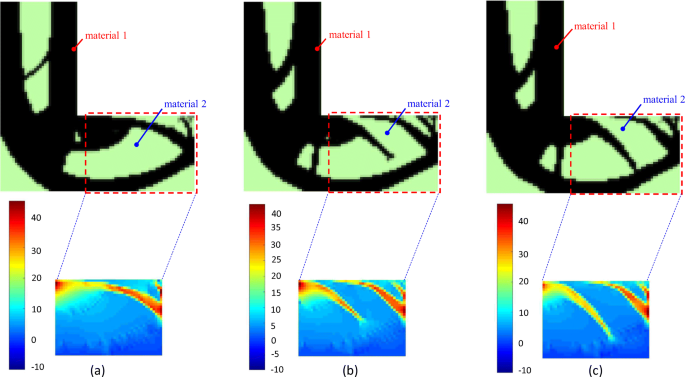
Optimized layouts and the corresponding contour plots of the first principal stress for cases D–F. a Case D, b Case E, c Case F

While for cases E and F, as shown in Fig. 16 (b) and (c), in which isotropic and kinematic hardening is applied to material 2, respectively, a noticeable change can be observed in the final topologies. The top ties are replaced by a smeared-strut-and-tie microstructure as illustrated in Fig. 17. The evolutionary histories of the objective function are shown in Fig. 18.

Strut-and-tie, smeared-strut-and-tie analogy for cases D–F. a Case D, b Case E, c Case F

Evolutionary histories of objective function for the cantilever beam with a circular opening. a Case A, b Case B, c Case C, d Case D, e Case E, f Case F
7 Conclusion and discussion
In this paper, a framework for multiphase material nonlinear topology optimisation is developed, implemented and validated. This new framework offers the flexibility that highly desired in complex composite structural optimization when each material has different nonlinear characteristics and hardening behaviours. As in this type of multiphase material nonlinear optimization, each material phase will not only associate with different plasticity models but also following different hardening rule so that each material elastoplastic properties can be closely characterized during the optimization process. In some practical design optimizations, having the flexibility of modelling the different actual material elastoplasticity, for example, von Mises plasticity with isotropic hardening for one material, while Drucker-Prager plasticity with kinematic hardening for the other, will lead to a better approximation of the real optimum design. Few studies focused on this area, and even fewer studies achieved this level of flexibilities that come with the proposed framework.
In supporting the proposed framework, a modified path-dependent adjoint sensitivity analysis is developed for calculating the design sensitivities when the two-phase elastoplastic materials are associated with various hardening rules.
As demonstrated in the examples, the proposed framework is effective, versatile and highly adaptive to the different elastoplastic and hardening models. The results of the example presented in this paper have also revealed the impact on the resulting topology when adopting different plasticity models and hardening rules in a composite structural optimization which has also demonstrated the flexibility of adapting to different material combinations for modern composite structures. Some of the topologies produced by the proposed method are novel yet fulfil the engineering common sense when looking into the details of microstructures.
References
Bendsøe MP, Sigmund O (1999) Material interpolation schemes in topology optimization. Arch Appl Mech (Ingenieur Archiv) 69(9–10):635–654
Bogomolny M, Amir O (2012) Conceptual design of reinforced concrete structures using topology optimization with elastoplastic material modeling. Int J Numer Methods Eng 90(13):1578–1597
Bruggi M (2009) Generating strut-and-tie patterns for reinforced concrete structures using topology optimization. Comput Struct 87(23):1483–1495
Bruggi M (2010) On the automatic generation of strut and tie patterns under multiple load cases with application to the aseismic design of concrete structures. Adv Struct Eng 13(6):1167–1181
Guan H (2005) Strut-and-tie model of deep beams with web openings - an optimisation approach. Struct Eng Mech 19(4):361–380
Huang X, Xie YM (2009) Bi-directional evolutionary topology optimization of continuum structures with one or multiple materials. Comput Mech 43(3):393–401
Kato J et al (2015) Analytical sensitivity in topology optimization for elastoplastic composites. Struct Multidiscip Optim 52(3):507–526
Li M, Zhang H (2018) Topology optimization of structures with elasto-plastic strain hardening material modeling. Springer International Publishing, Cham
Li L, Zhang G, Khandelwal K (2017) Design of energy dissipating elastoplastic structures under cyclic loads using topology optimization. Struct Multidiscip Optim 56(2):391–412
Liu S, Qiao H (2011) Topology optimization of continuum structures with different tensile and compressive properties in bridge layout design. Struct Multidiscip Optim 43:369–380
Luo Y, Kang Z (2012) Topology optimization of continuum structures with Drucker–Prager yield stress constraints. Comput Struct 90-91:65–75
Luo Y et al (2015) Topology optimization of reinforced concrete structures considering control of shrinkage and strength failure. Comput Struct 157:31–41
Maute K, Schwarz S, Ramm E (1998) Adaptive topology optimization of elastoplastic structures. Struct Optim 15(2):81–91
Michaleris P, Tortorelli DA, Vidal CA (1994) Tangent operators and design sensitivity formulations for transient non-linear coupled problems with applications to elastoplasticity. Int J Numer Methods Eng 37(14):2471–2499
Nakshatrala PB, Tortorelli DA (2015) Topology optimization for effective energy propagation in rate-independent elastoplastic material systems. Comput Methods Appl Mech Eng 295:305–326
Querin O, Victoria Nicolás M, Martí-Montrull P (2010) Topology optimization of truss-like continua with different material properties in tension and compression. Struct Multidiscip Optim 42:25–32
Schwarz S, Maute K, Ramm E (2001) Topology and shape optimization for elastoplastic structural response. Comput Methods Appl Mech Eng 190(15):2135–2155
Svanberg K (1987) The method of moving asymptotes—a new method for structural optimization. Int J Numer Methods Eng 24(2):359–373
Swan CC, Kosaka I (1997) Voigt–Reuss topology optimization for structures with nonlinear material behaviors. Int J Numer Methods Eng 40(20):3785–3814
Victoria M, Querin OM, Martí P (2011) Generation of strut-and-tie models by topology design using different material properties in tension and compression. Struct Multidiscip Optim 44(2):247–258
Wallin M, Jönsson V, Wingren E (2016) Topology optimization based on finite strain plasticity. Struct Multidiscip Optim 54(4):783–793
Xia L, Fritzen F, Breitkopf P (2017) Evolutionary topology optimization of elastoplastic structures. Struct Multidiscip Optim 55(2):569–581
Yoon GH, Kim YY (2007) Topology optimization of material-nonlinear continuum structures by the element connectivity parameterization. Int J Numer Methods Eng 69(10):2196–2218
Yuge K, Kikuchi N (1995) Optimization of a frame structure subjected to a plastic deformation. Struct Optim 10(3):197–208
Zhang G, Li L, Khandelwal K (2017) Topology optimization of structures with anisotropic plastic materials using enhanced assumed strain elements. Struct Multidiscip Optim 55(6):1965–1988
Acknowledgements
The authors would like to express their special gratitude to the supports from the Royal Academy of Engineering-Visiting Professor (VP2021\7\12); Royal Academy of Engineering-Industrial Fellowship (IF\192023); National Nature Science Foundation of China (51768008); British Council and Ministry of Education, China (UK-China-BRI Countries Education Partnership Initiative); Lawrence Ho Research fund, China Postdoctoral Science Foundation Project (2017M613273XB); and Nature Science Foundation of Guangxi Zhuang Autonomous Region (2019JJA160137) and Liuzhou Scientific Research and Technology Development Plan (2017 BC40202).
Author information
Authors and Affiliations
Corresponding author
Ethics declarations
Conflict of interest
The authors declare that they have no conflict of interest.
Replication of results
All presented results were obtained using a set of Matlab codes that are available upon request.
Additional information
Responsible Editor: Shikui Chen
Publisher's note
Springer Nature remains neutral with regard to jurisdictional claims in published maps and institutional affiliations.
Rights and permissions
Open Access This article is licensed under a Creative Commons Attribution 4.0 International License, which permits use, sharing, adaptation, distribution and reproduction in any medium or format, as long as you give appropriate credit to the original author(s) and the source, provide a link to the Creative Commons licence, and indicate if changes were made. The images or other third party material in this article are included in the article's Creative Commons licence, unless indicated otherwise in a credit line to the material. If material is not included in the article's Creative Commons licence and your intended use is not permitted by statutory regulation or exceeds the permitted use, you will need to obtain permission directly from the copyright holder. To view a copy of this licence, visit http://creativecommons.org/licenses/by/4.0/.
About this article

Cite this article
Li, M., Deng, Y., Zhang, H. et al. Topology optimization of multi-material structures with elastoplastic strain hardening model. Struct Multidisc Optim 64, 1141–1160 (2021). https://doi.org/10.1007/s00158-021-02905-3
Received:
Revised:
Accepted:
Published:
Issue Date:
DOI: https://doi.org/10.1007/s00158-021-02905-3