Hardy spaces associated to generalized Hardy operators and applications

Abstract

In this paper, we will study the Hardy and BMO spaces associated to the generalized Hardy operator $L_{\alpha }= (-\Delta )^{\alpha /2}+a|x|^{-\alpha }$. Similarly to the classical Hardy and BMO spaces, we will prove that our new function spaces will enjoy some important results such as molecular decomposition and duality. As applications, we show the boundedness of the spectral multiplier of Laplace transform type and the Sobolev norm inequalities involving the generalized Hardy operator.

1 Introduction

In this paper, we consider the following generalized Hardy operators on ${\mathbb {R}}^n, n\in {\mathbb {N}}$,

$$\begin{aligned} L_{\alpha }= (-\Delta )^{\alpha /2}+a|x|^{-\alpha } \quad \text {with} \quad 0<\alpha <\min \{2, n\} \ \ \text {and} \ \ \quad a\ge a^*, \end{aligned}$$

(1)

where

$$\begin{aligned} a^*=-\frac{2^\alpha \Gamma ((d+\alpha )/4)^2}{\Gamma ((d-\alpha )/4)^2}. \end{aligned}$$

The constant $a^*$ is reasoned by the sharp constant in the following Hardy-type inequality

$$\begin{aligned} \int _{{\mathbb {R}}^n} |x|^{-\alpha }|u(x)|^2dx \le -\frac{1}{a^*}\int _{{\mathbb {R}}^n} |\xi |^\alpha |{\widehat{u}}(\xi )|^2d\xi , \ \ \ \ \ u\in C_0^\infty ({\mathbb {R}}^n), \end{aligned}$$

where ${\widehat{u}}$ denotes the Fourier transform of u. Hence, the condition $a\ge a^*$ guarantees that the operator $L_{\alpha }$ is non-negative. See for example [12].

Following [12], we set

$$\begin{aligned} \Psi _{\alpha ,n}(\delta )=-2^\alpha \frac{\Gamma (\frac{\delta +\alpha }{2})\Gamma (\frac{n-\delta }{2})}{\Gamma (\frac{n-\delta -\alpha }{2})\Gamma (\frac{\delta }{2})}, \ \ \ \ \ \ \delta \in (-\alpha , (n-\alpha )/2]\backslash \{0\}, \end{aligned}$$

and $\Psi _{\alpha ,n}(0)=0$.

It was proved in [12] that the function $\Psi _{\alpha ,n}$ is continuous and strictly decreasing in $(-\alpha , (n-\alpha )/2]$ with

$$\begin{aligned} \lim \limits _{\delta \rightarrow -\alpha } \Psi _{\alpha ,n}(\delta )=\infty \ \ \ \ \text {and} \ \ \ \Psi _{\alpha ,n}\left( \frac{n-\alpha }{2}\right) =a^*. \end{aligned}$$

Therefore, for any $a\ge a^*$ we define

$$\begin{aligned} \sigma :=\Psi _{\alpha ,n}^{-1}(a) \end{aligned}$$

(2)

so that $\sigma \in (-\alpha , (n-\alpha )/2]$.

The operator $L_{\alpha }$ can be viewed as a Schödinger operator of the fractional Laplacian $L_{\alpha }= (-\Delta )^{\alpha /2} +V$ with $V=a|x|^{-\alpha }$. In this case the potential V might be negative. Therefore, the heat kernel of $L_{\alpha }$ fails to satisfy the Poisson upper bounds.

The main aim of this paper is twofold. Firstly, we develop the theory of Hardy spaces $H^p_{L_{\alpha }}({\mathbb {R}}^n)$ associated to the operator $L_{\alpha }$ for $\frac{n}{n+\alpha }<p\le 1$. We show that the Hardy spaces admit molecular decomposition which is similar to the classical Hardy space. Then we also prove the duality result of the Hardy spaces $H^p_{L_{\alpha }}({\mathbb {R}}^n)$ and new BMO spaces. See Sect. 3. Secondly, as applications we obtained our result to prove the boundedness of the spectral multiplier of Laplace transform type and the Sobolev norm equivalence involving the generalized Hardy operators $L_{\alpha }$.

We would like to point out that the ideas of Hardy spaces associated to operators in this paper are not new. In [2], such a function space spaces associated to L was investigated under the condition that the heat kernel of L enjoys a pointwise Gaussian upper bound. The theory of Hardy spaces associated to non-negative self adjoint operators satisfying Davies–Gaffney estimates was then introduced in [14]. We note that the Davies–Gaffney estimates do not require any pointwise estimates. For further information about this research direction, we refer [2, 3, 9, 11, 13, 14, 16] and the references therein. Although the approach in our paper bases on those in [11, 14], a number of important improvements and modifications are needed. This is because the kernel of $L_{\alpha }$ does not satisfy either Poisson upper bound or the Davies–Gaffney estimates. See Theorems 2.1 and 2.2. This also reasons why we are able to develop the theory of the Hardy spaces $H^p_{L_{\alpha }}({\mathbb {R}}^n)$ for $\frac{n}{n+\alpha }<p\le 1$ instead of $0<p\le 1$ as in [9, 16].

Regarding the second aim we would like to mention that the Sobolev norm equivalence involving the generalized Hardy operators $L_{\alpha }$ is an interesting topics in PDEs. In [12], the $L^2$-norm equivalence $\Vert L_{\alpha }^s f\Vert _2\sim \Vert (\Delta )^{s\alpha /2}f\Vert _2$ with $s\in (0,2]$ was obtained. The result was extended in [17] to $p\ne 2$ for $s=2$ and $s\in (0,2), a\ge 0$. The remaining case $s\in (0,2), a\ge a^*$ was proved recently by D’Ancona and the first-named author [6]. In this paper, we use the new theory of Hardy spaces $H^p_{L_{\alpha }}$ to recover the inequality $\Vert L_{\alpha }^s f\Vert _p\lesssim \Vert (\Delta )^{s\alpha /2}f\Vert _p$ for $p\ne 2$, $s\in (0,2]$ and $a\ge a^*$. This provides new thoughts and new ideas involving the Sobolev norm equivalence problem.

The organization of the paper is as follows. Section 2 proves some kernel estimates, recalls some properties on the tent spaces introduced in [8] and gives the boundedness of the conical and vertical square functions associated to $L_{\alpha }$. The theory of Hardy spaces and BMO spaces will be given in Sect. 3. In this section, we prove some important results such as molecular decomposition for the Hardy spaces and the duality result on the Hardy spaces and BMO type spaces. Finally, as applications, in Sect. 4 we will prove the boundedness of the spectral multiplier of $L_{\alpha }$ and an inequality regarding the Sobolev norm equivalence involving the operator $L_{\alpha }$.

Throughout the paper, we always use C and c to denote positive constants that are independent of the main parameters involved but whose values may differ from line to line. We will write $A\lesssim B$ if there is a universal constant C so that $A\le CB$ and $A\sim B$ if $A\lesssim B$ and $B\lesssim A$. We also denote

$$\begin{aligned} a\vee b =\max \{a,b\} \ \ \ \text {and} \ \ \ \ a \wedge b = \min \{a,b\} \end{aligned}$$

for $a,b \in {\mathbb {R}}$.

2 Preliminaries

2.1 Some kernel estimates

For a constant $\sigma \in {\mathbb {R}}$. We denote

$$\begin{aligned} D_\sigma (x,t)=\left( 1+\frac{t^\frac{1}{\alpha }}{|x|}\right) ^\sigma \end{aligned}$$

(3)

and

$$\begin{aligned} n_\sigma = {\left\{ \begin{array}{ll} \frac{n}{\sigma } &{}, \sigma > 0 \\ \infty &{}, \sigma \le 0. \end{array}\right. } \end{aligned}$$

We now recall the following heat kernel estimate in [4,5,6,7, 12, 15]

Theorem 2.1

Let $n\in {\mathbb {N}},0< \alpha < 2\wedge n, a \ge a^*, k\in {\mathbb {N}}\cup \{0\}$, and let $\sigma$ be defined as in (2). Let $p_{k,t}(x,y)$ be the kernel associated to the semi-group $L_{\alpha }^ke^{-tL_{\alpha }}$. Then there exist positive constant $C_k$ such that for all $t>0$ and $x,y \in {\mathbb {R}}^n \setminus \{0\}$,

$$\begin{aligned} p_{k,t}(x,y) \le C_k t^{-\left( k+\frac{n}{\alpha }\right) }D_{\sigma }(x,t) D_{\sigma }(y,t)\left( \frac{t^\frac{1}{\alpha }+|x-y|}{t^\frac{1}{\alpha }}\right) ^{-n-\alpha }. \end{aligned}$$

In what follows, given a ball B we denote $S_j(B) = 2^jB \setminus 2^{j-1}B$ for $j = 1,2,3,\dots$ and $S_0(B)=B$. For $f\in L^1_{\mathrm{loc}}({\mathbb {R}}^n)$ and a ball B, we denote

for $j=0,1,2\ldots .$

The following estimates are taken from [6].

Theorem 2.2

([6]) Let $L_{\alpha }$ be as in (1) with $\sigma$ defined by (2). Let $k\in {\mathbb {N}}\cup \{0\}$ and $T_t = \left( t^\alpha L_{\alpha }\right) ^k e^{-t^\alpha L_{\alpha }}$. Assume that $({n}_{\sigma })'<p\le q <{n}_{\sigma }$. Then for any ball B, for every $t>0$ and $j\in {\mathbb {N}}$ we have:

for all $f\in L^p({\mathbb {R}}^n)$ supported in B, and

for all $f\in L^p(S_j(B))$.

Lemma 2.3

Let $\sigma \in (-\infty ,n)$. For $r,t>0$, $x \in {\mathbb {R}}^n$ and $f \in L^2_{\mathrm{loc}}({\mathbb {R}}^n)$, we have

$$\begin{aligned} \int _{B(x,r)}D_{\sigma }(z,t)dz \lesssim \min \big \{t^\frac{n}{\alpha }+r^n, t^{\frac{\sigma }{\alpha }}r^{n-\sigma }+r^n\big \}, \end{aligned}$$

(4)

and

$$\begin{aligned} \int _{B(x,r)}|D_{\sigma }(z,t)f(z)|dz \lesssim t^{\frac{n}{2\alpha }}\Vert f\Vert _{L^2(B)}+\Vert f\Vert _{L^1(B(x,r)) }. \end{aligned}$$

(5)

Proof

We have

$$\begin{aligned} \int _{B(x,r)}D_{\sigma }(z,t)dz&=\int _{B(x,r)\cap B(0,t^\frac{1}{\alpha })}\left( 1+\frac{t^\frac{1}{\alpha }}{|z|}\right) ^\sigma dz\\&\quad +\int _{B(x,r)/B(0,t^\frac{1}{\alpha })}\left( 1+\frac{t^\frac{1}{\alpha }}{|z|}\right) ^\sigma dz\\&\lesssim \int _{B(x,r)\cap B(0,t^\frac{1}{\alpha })}\left( \frac{t^\frac{1}{\alpha }}{|z|}\right) ^\sigma dz+\int _{B(x,r)/B(0,t^\frac{1}{\alpha })}1 dz\\&\lesssim \min \big \{t^\frac{n}{\alpha }+r^n, t^{\frac{\sigma }{\alpha }}r^{n-\sigma }+r^n \big \}. \end{aligned}$$

Hence, the inequality (4) is proved.

For the estimate (5), we have

$$\begin{aligned} \int _{B(x,r)}|D_{\sigma }(z,t)f(z)|dz&=\int _{B(x,r)\cap B\left( 0,t^\frac{1}{\alpha }\right) }\left( 1+\frac{t^\frac{1}{\alpha }}{|z|}\right) ^\sigma |f(z)| dz\\&\quad +\int _{B(x,r)/B(0,t^\frac{1}{\alpha })}\left( 1+\frac{t^\frac{1}{\alpha }}{|z|}\right) ^\sigma |f(z)| dz\\&\lesssim \int _{B(x,r)\cap B(0,t^\frac{1}{\alpha })}\left( \frac{t^\frac{1}{\alpha }}{|z|}\right) ^\sigma |f(z)|dz\\&\quad +\int _{B(x,r)/B(0,t^\frac{1}{\alpha })}|f(z)| dz\\&\lesssim \left[ \int _{B(x,r)\cap B(0,t^\frac{1}{\alpha })}\left( \frac{t^\frac{1}{\alpha }}{|z|}\right) ^{2\sigma }dz \right] ^\frac{1}{2}\Vert f\Vert _{L^2(B)}+\Vert f\Vert _{L^1(B)} \\&\lesssim t^{\frac{n}{2\alpha }}\Vert f\Vert _{L^2(B(x,r))}+\Vert f\Vert _{L^1(B(x,r)) }. \end{aligned}$$

$\square$

2.2 Tent spaces

The tent spaces, which were first introduced in [8], become an effective tool in the study of function spaces in harmonic analysis including Hardy spaces. In this section we will recall the definitions of the tent spaces and their fundamental properties in [8]. We begin with some notations in [8].

• For $x\in {\mathbb {R}}^n$ and $\beta >0$, we denote

  $$\begin{aligned} \Gamma ^\beta (x):=\big \{(y,t)\in {\mathbb {R}}^n\times \left( 0,\infty \right) : |x-y| \le \beta t\big \}. \end{aligned}$$

  When $\beta =1$, we briefly write $\Gamma (x)$ instead of $\Gamma ^1(x)$.

• For any closed subset $F \subset {\mathbb {R}}^n$ , define

  $$\begin{aligned} R^\beta (F) = \cup _{x\in F} \Gamma ^\beta (x), \end{aligned}$$

  and we also denote $R^1(F)$ by R(F).

• If O is an open set in ${\mathbb {R}}^n$, then the tent over $\widehat{O}$ is defined as

  $$\begin{aligned} \widehat{O}=\left( R(O^c)\right) ^c. \end{aligned}$$

Let ${{\mathbb {R}}_+^{n+1}}= \{(y,t)\in {\mathbb {R}}^{n+1}, t>0\}$. For a measurable function F defined in ${{\mathbb {R}}_+^{n+1}}$, we define

$$\begin{aligned} A(F)(x)= & {} \left( \int _{\Gamma (x)}|F(y,t)|^2\frac{dydt}{t^{n+1}}\right) ^\frac{1}{2},\\ C(F)(x)= & {} \underset{x\in B}{\sup }\left( \frac{1}{|B|}\int _{\widehat{B}}|F(y,t)|^2\frac{dydt}{t}\right) ^\frac{1}{2}, \end{aligned}$$

and

$$\begin{aligned} C_p(F)(x)=\underset{x\in B}{\sup }\frac{1}{|B|^{\frac{1}{p}-\frac{1}{2}}}\left( \int _{\widehat{B}}|F(y,t)|^2\frac{dydt}{t}\right) ^\frac{1}{2} \ \ \ \text { for } 0 < p \le 1. \end{aligned}$$

The following definition is taken from [8].

Definition 2.4

(The tent spaces) The tent spaces are defined as follows.

• For $0<p < \infty$, we define $T_2^p:= \{F: \ A(F)\in L^p({\mathbb {R}}^n) \}$ with the norm $\Vert F\Vert _{T^p_2}= \Vert A(F)\Vert _{p}$ which is a Banach space for $1\le p<\infty$.

• For $p = \infty$, we define $T_2^\infty =\big \{F: \ C(F) \in L^\infty ({\mathbb {R}}^n) \big \}$ with the norm $\Vert F\Vert _{T_2^\infty ({\mathbb {R}}^n)}=\Vert C(F)\Vert _{\infty }$ which is a Banach space.

• For $0<p \le 1$, we define $T_2^{p,\infty }=\big \{F: \Vert C_p(F)\Vert _\infty <\infty \big \}$ with the norm $\Vert F\Vert _{T_2^{p,\infty }}=\Vert C_pF\Vert _\infty$. Obviously, $T^{1,\infty }_2=T_2^\infty$.

One of the most important properties of the tent spaces is atomic decomposition. We now recall the definition of atoms in the tent space $T_2^p$.

Definition 2.5

([8]) For $0<p\le 1$, a measurable function F on ${{\mathbb {R}}_+^{n+1}}$ is said to be a $T_2^p$-atom if there exists a ball $B\in {\mathbb {R}}^n$ such that F is supported in $\widehat{B}$ and

$$\begin{aligned} \int _{{\mathbb {R}}_+^{n+1}}|F(x,t)|^2\frac{dx dt}{t^{n+1}} \le |B|^{1-\frac{2}{p}}. \end{aligned}$$

Then we have:

Lemma 2.6

Let $0<p\le 1$. For every $F\in T_2^p$ there exist a constant $C_p>0$, a sequence of numbers $\big \{\lambda _j\big \}_{j=0}^\infty$ and a sequence of $T_2^p$-atom $\big \{A_j\big \}_{j=0}^\infty$ such that

$$\begin{aligned} F= \sum _{j=0}^{\infty }\lambda _jA_j \text { in} T_2^p \text { a.e in } {{\mathbb {R}}_+^{n+1}} \end{aligned}$$

and

$$\begin{aligned} \sum _{j=0}^{\infty }|\lambda _j|^p\le C_p\Vert F\Vert ^p_{T_2^p({\mathbb {R}}^n)}. \end{aligned}$$

Furthermore, if $F \in T_2^p \cap T_2^2$, then the sum also converges in $T^2_2$.

Proof

See Proposition 5 in [8] and Corollary 3.1 in [16]. $\square$

We also recall duality results of the tent spaces.

Proposition 2.7

• (i) The following inequality holds, whenever $f\in T_2^1$ and $g \in T_2^\infty$:

  $$\begin{aligned} \int _{{\mathbb {R}}^{n+1}_{+}}|f(x,t)g(x,t)|\frac{dxdt}{t}\le c\int _{{\mathbb {R}}^n}A(f)(x)C(g)(x)dx. \end{aligned}$$

• (ii) Suppose $1<p< \infty$, $f \in T^p_2$ and $g\in T_2^{p'}$ with $\frac{1}{p}+\frac{1}{p'}=1$ then

  $$\begin{aligned} \int _{{\mathbb {R}}_{+}^{n+1}}|f(y,t)g(y,t)|\frac{dydt}{t}\le \int _{{\mathbb {R}}^n}A(f)(x)A(g)(x)dx. \end{aligned}$$

• (iii) If $0 <p \le 1$, then the dual space of $T_2^p$ is $T_2^{p,\infty }$. More precisely, the pairing

  $$\begin{aligned} \left\langle f,g \right\rangle =\int _{{\mathbb {R}}^{n+1}_{+}}f(x,t)g(x,t)\frac{dxdt}{t} \end{aligned}$$

  realizes $T_2^{p,\infty }$ as the dual of $T_2^p$.

Proof

We refer Theorems 1 and 2 in [8] for the proof of (i) and (ii), and Proposition 3.2 in [19] for the proof of (iii). $\square$

2.3 Square functions

For $f\in L^2({\mathbb {R}}^n)$ and $x\in {\mathbb {R}}^n$, we define the vertical square function and the area square function by

$$\begin{aligned} G_{L_{\alpha }}f(x):= \left( \int _{0}^\infty \big | t^\alpha L_{\alpha }e^{-t^\alpha L_{\alpha }}f(x)\big |^2\frac{dt}{t} \right) ^\frac{1}{2} , \end{aligned}$$

and

$$\begin{aligned} S_{L_{\alpha }}(f)(x):= \left( \int _{0}^\infty \int _{B(x,t)} \Big |t^\alpha L_{\alpha }e^{-t^\alpha L_{\alpha }}f(y)\Big |^2\frac{dydt}{t^{n+1}} \right) ^\frac{1}{2}. \end{aligned}$$

Theorem 2.8

Let $L_{\alpha }$ be as in (1) with $\sigma$ defined by (2). For all $\left( {n}_{\sigma }\right) '< p < {n}_{\sigma }$, we have

$$\begin{aligned} \big \Vert G_{L_{\alpha }}f\big \Vert _p \sim \Vert f\Vert _p. \end{aligned}$$

Proof

The proof of this theorem is similar to that of [6, Theorem 4.1] and we omit the detail. $\square$

For the boundedness of the area square function $S_{L_{\alpha }}$ we have the following result.

Theorem 2.9

The area square function $S_{L_{\alpha }}$ is bounded on $L^p({\mathbb {R}}^n)$ for all $\left( {n}_{\sigma }\right) '< p < {n}_{\sigma }$.

In order to prove the theorem, we need the following result in [1].

Theorem 2.10

Let $1\le p_0<2$ and T be sublinear operator which is bounded on $L^2({\mathbb {R}}^n)$. Assume that there exists a family of operators $\{ A_t\}_{t>0}$ satisfying that for every ball B and for all f supported in B

• (1)
  

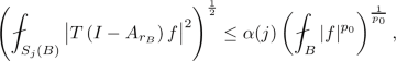
  when $j \ge 3$ and

• (2)
  

when $j \ge 2$ . If $\sum _{j=2}^\infty \alpha (j) 2^{jn} < \infty$, then T is bounded on $L^p({\mathbb {R}}^n)$ for all $p\in \left( p_0,2\right)$.

Proof of Theorem 2.9

For $\left( {n}_{\sigma }\right) '<p < 2$, we apply Theorem 2.10 with

$$\begin{aligned} \alpha (j)= \max \{2^{-j\alpha (1-\frac{1}{M+\alpha })},2^{-j(M\alpha -n)}\} \end{aligned}$$

and

$$\begin{aligned} A_{r_B}=I-\left( I-e^{-r_B^\alpha L_{\alpha }}\right) ^M, \end{aligned}$$

where M is a fixed constant such that $M\in {\mathbb {N}}$ and $M>\frac{n}{\alpha }$. We have (2) from Theorem 2.10 is a direct result of Theorem 2.2. Hence, we have to show that for all $j \ge 3$, balls $B=B(x_B,r_B)$ and $f\in L^p({\mathbb {R}}^n)$ supported in B, it holds that

where $\sum _{j=2}^\infty 2^{nj}\alpha (j) <\infty$. First, we write

We will now study $A_1$. Let

$$\begin{aligned} F_j(B):=\left\{ z\in {\mathbb {R}}^n: \text {there is } x\in S_j(B) \text { such that } |x-z| < \frac{|x-x_B|}{4} \right\} . \end{aligned}$$

Then $F_j(B) \subset S_{j-1}(B)\cup S_j(B) \cup S_{j+1}(B)=:Y_j(B).$ Hence, using the following identity

$$\begin{aligned} \left( I-e^{-r_B^\alpha L_{\alpha }}\right) ^M= \int _{[0,r_B^\alpha ]^M} L_{\alpha }^M e^{-(s_1+\ldots +s_M)L_{\alpha }} d\mathbf {s}, \end{aligned}$$

(6)

where $d\mathbf {s}=ds_1 \ldots ds_M$.

we have

$$\begin{aligned} A_1&\le \left( \frac{1}{|2^jB|}\int _{F_j(B)}\int _{0}^{\frac{d(x_B,x)}{4}}\big |t^\alpha L_{\alpha }e^{-t^\alpha L_{\alpha }}\left( I-e^{-r_B^\alpha L_{\alpha }}\right) ^Mf(y)\big |^2\frac{dt}{t}dy\right) ^\frac{1}{2}\\&\lesssim \left( \frac{1}{|2^jB|}\int _{Y_j(B)}\int _{0}^{2^jr_B}\Big |t^\alpha L_{\alpha }e^{-t L_{\alpha }}\int _{[0,r_B^\alpha ]^M} L_{\alpha }^M e^{-(s_1+\ldots +s_M)L_{\alpha }}f(y) d\mathbf {s}\Big |^2\frac{dt}{t}dy\right) ^\frac{1}{2} \end{aligned}$$

In order to estimate $A_1$, we need only to estimate the term

$$\begin{aligned} \left( \frac{1}{|2^jB|}\int _{S_j(B)}\int _{0}^{2^jr_B}\Big |t^\alpha L_{\alpha }e^{-t^\alpha L_{\alpha }}\int _{[0,r_B^\alpha ]^M} L_{\alpha }^M e^{-(s_1+\cdots +s_M)L_{\alpha }}f(y) d\mathbf {s}\Big |^2\frac{dt}{t}dy\right) ^{\frac{1}{2}}, \end{aligned}$$

since the estimates of the integrals over $S_{j-1}$ and $S_{j+1}$ can be done similarly.

Let $\tau = t^\alpha + s_1+\cdots +s_M$. By using Minkowski’s inequality we have

$$\begin{aligned}&\left( \frac{1}{|2^jB|}\int _{S_j(B)}\int _{0}^{2^jr_B}\Big |t^\alpha L_{\alpha }e^{-t^\alpha L_{\alpha }}\int _{[0,r_B^\alpha ]^M} L_{\alpha }^M e^{-(s_1+\cdots +s_M)L_{\alpha }}f(y) d\mathbf {s}\Big |^2 \frac{dt}{t}dy\right) ^\frac{1}{2}\\&\quad \lesssim \frac{1}{|2^jB|^\frac{1}{2}}\int _{[0,r_B^\alpha ]^M}\\&\qquad \left( \int _{0}^{2^jr_B}\int _{S_j(B)}\big |t^\alpha L_{\alpha }^{M+1} e^{-(t^\alpha +s_1+\cdots +s_M)L_{\alpha }}f(y)\big |^2dy\frac{dt}{t}\right) ^\frac{1}{2} d\mathbf {s}\\&\quad \lesssim \int _{[0,r_B^\alpha ]^M} \left( \int _{0}^{2^jr_B}\frac{1}{|2^jB|}\int _{S_j(B)}\big |t^\alpha L_{\alpha }^{M+1} e^{-\tau L_{\alpha }}f(y)\big |^2dy\frac{dt}{t} \right) ^\frac{1}{2} d\mathbf {s} \end{aligned}$$

In addition, by using Theorem 2.2 and the fact $\tau \lesssim (2^jr_B)^\alpha$ in this situation, we have

Then, by a straightforward calculation we have

which implies

We now take care of $A_2$. Let $B_t=B(x_B,4t)$, we have

In case of $B_1$ and $B_2$ we have $t> r_B$ and hence $B \subset B(x_B,t)$. Therefore, $f=f.1_{B(x_B,t)}$. Let $\tau =t^\alpha +s_1+\ldots +s_M$. By using Theorem 2.2 and Minkowski’s inequality we have

Hence, we have

Similarly, for all $k\in {\mathbb {N}}$ with $k \ge 2$, we have

$$\begin{aligned}&\frac{1}{|2^jB|^\frac{1}{2}}\left( \int _{2^{j-2}r_B}^\infty \left( \int _{S_k(B_t)}\Big |t^\alpha L_{\alpha }e^{-t^\alpha L_{\alpha }}\left( I-e^{-r_B^\alpha L_{\alpha }}\right) ^M f(y)\Big |^2dy\right) \frac{dt}{t}\right) ^\frac{1}{2} \\&\quad \lesssim \frac{1}{|2^jB|^\frac{1}{2}}\left( \int _{2^{j-2}r_B}^\infty \int _{S_k(B_t)}\Big |t^\alpha L_{\alpha }e^{-t^\alpha L_{\alpha }} \int _{[0,r_B^\alpha ]^M}L_{\alpha }^M e^{-(s_1+\ldots +s_M)L_{\alpha }}f(y) d\mathbf {s}\Big |^2 dy\frac{dt}{t}\right) ^\frac{1}{2}. \end{aligned}$$

In addition, by using Theorem 2.2 and Minkowski’s inequality,

Therefore,

Hence, using Theorem 2.10 we conclude that $S_{L_{\alpha }}$ is bounded on $L^p({\mathbb {R}}^n)$ for all $p \in \left( {n}_{\sigma }',2\right)$. Let ${\mathcal {M}}$ be the Hardy–Litllewood maximal operator. By using Fubini’s theorem and Hölder inequality, and for $p\in (2,{n}_{\sigma })$, for any $h\in L^{(\frac{p}{2})'}({\mathbb {R}}^n)$, we have

$$\begin{aligned} \int _{{\mathbb {R}}^n}\left( S_{L_{\alpha }}f(x)\right) ^2h(x)dx&\le \int _{{\mathbb {R}}^n}\int _0^\infty \int _{B(x,t)}\left( t^\alpha L_{\alpha }e^{-t^\alpha L_{\alpha }}f(y)\right) ^2 h(x) \frac{dydt}{t^{n+1}}dx\\&\le \int _{{\mathbb {R}}^n}\int _0^\infty \int _{B(y,t)}\left( t^\alpha L_{\alpha }e^{-t^\alpha L_{\alpha }}f(y)\right) ^2 h(x) \frac{dxdt}{t^{n+1}}dy \\&\lesssim \int _{{\mathbb {R}}^n}\int _0^\infty \left( t^\alpha L_{\alpha }e^{-t^\alpha L_{\alpha }}f(y)\right) ^2{\mathcal {M}}(h)(y)\frac{dt}{t}dy\\&\lesssim \int _{{\mathbb {R}}^n}\left( G_{L_{\alpha }}f(y)\right) ^2 {\mathcal {M}}(h)(y)dy \le \big \Vert G_{L_{\alpha }}(f)\big \Vert _{L^p}^2\big \Vert {\mathcal {M}}(h)\big \Vert _{L^{(\frac{p}{2})'}}. \end{aligned}$$

By using Theorem 2.8 we have $G_{L_{\alpha }}$ is bounded on $L^p$. In addition, we have $\left( \frac{p}{2}\right) '>1$. Hence ${\mathcal {M}}$ is bounded on $L^{\left( \frac{p}{2}\right) '}$. Therefore,

$$\begin{aligned} \int _{{\mathbb {R}}^n}\left( S_{L_{\alpha }} f(x)\right) ^2h(x)dx \lesssim \Vert f|\Vert ^2_{L^p({\mathbb {R}}^n)}\Vert h\Vert _{L^{(\frac{p}{2})'}}, \end{aligned}$$

which imply that $S_{L_{\alpha }}$ is bounded on $L^p({\mathbb {R}}^n)$ for all $p \in \left( 2, \frac{n}{\sigma }\right)$. Thus, Theorem 2.9 is proved. $\square$

3 Hardy spaces and BMO spaces associated to generalized Hardy operators

In this section, we always assume that $L_{\alpha }$ is the operator defined by (1) with $\sigma$ defined by (2). Our approach based on the approaches in [2, 3, 9,10,11, 14, 16, 19]. However, since the heat kernel estimates of $L_{\alpha }$ are weaker than those in existing settings, new ideas and modifications are required.

3.1 Hardy spaces associated to generalized Hardy operators

We now follow [2] to define the new Hardy spaces via the area square function associated to $L_{\alpha }$.

Definition 3.1

For $0<p\le 1$, we set

$$\begin{aligned} {\mathbb {H}}^p_{S_{L_{\alpha }}}({\mathbb {R}}^n) =\Big \{f\in L^2({\mathbb {R}}^n): S_{L_{\alpha }}(f) \in L^p({\mathbb {R}}^n)\Big \}. \end{aligned}$$

We then defined the Hardy space $H^p_{S_{L_{\alpha }}}({\mathbb {R}}^n)$ to be the completion of the set ${\mathbb {H}}^p_{S_{L_{\alpha }}}({\mathbb {R}}^n)$ under the norm

$$\begin{aligned} \Vert f\Vert _{{\mathbb {H}}^p_{S_{L_{\alpha }}}({\mathbb {R}}^n)}:= \big \Vert S_{L_{\alpha }}(f)\big \Vert _p. \end{aligned}$$

Similarly to the classical case, we will show that our new Hardy spaces admit molecular decomposition property. We adapt ideas in [9, 13, 14] to introduce a notion of molecules in our setting.

Definition 3.2

For $0< p \le 1$, we defined $m(x) \in L^2({\mathbb {R}}^n)$ to be a $(p,2,M, \epsilon )_{L_{\alpha }}$-molecule associated to $L_{\alpha }$, if there exist a function $b \in D\left( L^M\right)$ and a ball $B=B(x_B,r_B)$ such that

• (i) $m = L_{\alpha }^M b$.

• (ii) For every $k=0,1,..,M$ and $j \in {\mathbb {N}}$ one has

  $$\begin{aligned} \big \Vert \left( r^\alpha _B L_{\alpha }\right) ^k b \big \Vert _{L^2(S_j(B))} \le 2^{-j \epsilon }r_B^{\alpha M}|2^jB|^{\frac{1}{2}-\frac{1}{p}}. \end{aligned}$$

Then we can define the Hardy spaces associated to $L_{\alpha }$ via molecular decomposition. Furthermore, we have

$$\begin{aligned} \begin{aligned} \Vert m\Vert _{L^2({\mathbb {R}}^n)}&\le \sum _{j=0}^\infty \Vert L_{\alpha }^M b\Vert _{L^2(S_j(B))} \\&\le \sum _{j=0}^\infty 2^{-j \epsilon }|B|^{\frac{1}{2}-\frac{1}{p}}\\&\le c |B|^{\frac{1}{2}-\frac{1}{p}}. \end{aligned} \end{aligned}$$

(7)

Definition 3.3

Given $0 < p \le 1$ and $\epsilon >0$, we say that $f= \sum _i \lambda _i m_i$ is an molecular $(p,2,M,\epsilon )_{L_{\alpha }}$-representation of f if $\left( \sum _{j=0}^\infty |\lambda _i|^p\right) ^\frac{1}{p} <\infty$, each $m_j$ is a $\left( p,2,M,\epsilon \right)$-molecule, and the sum converges in $L^2({\mathbb {R}}^n)$. Set

$$\begin{aligned} {\mathbb {H}}^p_{L_{\alpha }, \mathrm{mol},M,\epsilon }({\mathbb {R}}^n) = \big \{f \in L^2({\mathbb {R}}^n) : \text {f has a } (p,2,M, \epsilon )_{L_{\alpha }}\text {-representation} \big \} \end{aligned}$$

for $0<p\le 1$, with the norm given by

$$\begin{aligned}&\Vert f\Vert _{{\mathbb {H}}^p_{L_{\alpha },\mathrm{mol},M,\epsilon }({\mathbb {R}}^n)}\\&\quad = \inf \left\{ \left( \sum _{i=0}^{\infty } |\lambda _i|^p\right) ^\frac{1}{p}:f=\sum _{i=0}^{\infty }\lambda _im_i \text { is a }(p,2,M,\epsilon )_{L_{\alpha }}-representation\right\} . \end{aligned}$$

For $0<p\le 1$, the space $H^p_{L_{\alpha }, \mathrm{mol},M,\epsilon }({\mathbb {R}}^n)$ is defined to be the completion of ${\mathbb {H}}^p_{L_{\alpha },\mathrm{mol},M,\epsilon }({\mathbb {R}}^n)$ with respect to the norm $\Vert .\Vert _{{\mathbb {H}}^p_{{L_{\alpha }},\mathrm{mol},M,\epsilon }({\mathbb {R}}^n)}$.

The main result in this section is formulated by the following theorem.

Theorem 3.4

Let $\frac{n}{n +\alpha } <p\le 1$, $\epsilon =\alpha +n -\frac{n}{p}$ and $M>\frac{n}{\alpha p}$. Then the two Hardy spaces $H^p_{L_{\alpha },\mathrm{mol},M,\epsilon }({\mathbb {R}}^n)$ and $H^p_{S_{L_{\alpha }}}({\mathbb {R}}^n)$ coincide with equivalent norms.

Proof

Theorem 3.4 is a direct consequence of Proposition 3.6 and Proposition 3.8 below. $\square$

To begin the proof of Theorem 3.4, we state the following lemma. The proof of this lemma is similar to that of Lemma 3.3 in [13] and we omit it here.

Lemma 3.5

Fix $\frac{n}{n +\alpha } <p\le 1$, $\epsilon >0$ and $M >\frac{n}{\alpha p} .$ Assume that T is a linear operator , or non-negative sublinear operator of weak-type (2, 2), and that for every $(p,2,M, \epsilon )_{L_{\alpha }}$-molecule m, we have $\Vert Tm\Vert _{L^p{({\mathbb {R}}^n)}} \le C$ with constant C independent of m. Then T is bounded from ${\mathbb {H}}^p_{L_{\alpha }, \mathrm{mol},M,\epsilon }({\mathbb {R}}^n)$ to $L^p({\mathbb {R}}^n)$, and

$$\begin{aligned} \Vert Tf\Vert _{L^p({\mathbb {R}}^n)} \le C \Vert f\Vert _{H^p_{L_{\alpha }, \mathrm{mol},M,\epsilon }({\mathbb {R}}^n)}. \end{aligned}$$

Hence, by using density argument, T extends to a bounded operator from $H^p_{L_{\alpha }, \mathrm{mol}, M,\epsilon }({\mathbb {R}}^n)$ to $L^p({\mathbb {R}}^n)$.

Proposition 3.6

For $p\in \left( \frac{n}{n+\alpha },1\big ]\right.$, $\epsilon >0$ and $M> \frac{n}{\alpha p}$, we have

$$\begin{aligned} {\mathbb {H}}^p_{L_{\alpha },\mathrm{mol},M,\epsilon }({\mathbb {R}}^n) \hookrightarrow {\mathbb {H}}^p_{S_{L_{\alpha }}}({\mathbb {R}}^n), \end{aligned}$$

and hence,

$$\begin{aligned} H^p_{L_{\alpha },\mathrm{mol},M,\epsilon }({\mathbb {R}}^n) \hookrightarrow H^p_{S_{L_{\alpha }}}({\mathbb {R}}^n). \end{aligned}$$

Proof

Fix $p\in \Big (\frac{n}{n+\alpha },1\big ]$, $\epsilon >0$ and $M> \frac{n}{\alpha p}$. By Lemma 3.5, it suffices to prove that there exists $C>0$ such that

$$\begin{aligned} \big \Vert S_{L_{\alpha }}(m)\big \Vert _{L^p({\mathbb {R}}^n)}\le C \end{aligned}$$

for every $(p,2,M,\epsilon )_{L_{\alpha }}$-molecule m.

Let m be a $(p,2,M,\epsilon )_{L_{\alpha }}$-molecule and $B(x_B,r_B)$ be the ball associated to m. Then we have

$$\begin{aligned} \Vert S_{L_{\alpha }} m\Vert _p^p&= \int _{{\mathbb {R}}^n} \left( \iint _{\Gamma (x)} \big |t^{\alpha } L_{\alpha } e^{-t^{\alpha } L_{\alpha }} m(y)\big |^2 \frac{dydt}{t^{n+1}}\right) ^\frac{p}{2} dx \\&\le \int _{{\mathbb {R}}^n}\left( \iint _{\Gamma (x)}1_{2B\times (0,2r_B)}\big |t^{\alpha } L_{\alpha } e^{-t^{\alpha } L_{\alpha }} m(y)\big |^{2}\frac{dydt}{t^{n+1}}\right) ^\frac{p}{2}dx\\&\quad + \sum _{j=2}^\infty \int _{{\mathbb {R}}^n}\left( \iint _{\Gamma (x)}1_{S_j(B)\times (0,r_B)}\big |t^{\alpha } L_{\alpha } e^{-t^{\alpha } L_{\alpha }} m(y)\big |^{2}\frac{dydt}{t^{n+1}}\right) ^\frac{p}{2}dx\\&\quad +\sum _{j=2}^\infty \int _{{\mathbb {R}}^n}\left( \iint _{\Gamma (x)}1_{S_j(B)\times (r_B,2^{j}r_B)}\big |t^{\alpha } L_{\alpha } e^{-t^{\alpha } L_{\alpha }} m(y)\big |^{2}\frac{dydt}{t^{n+1}}\right) ^\frac{p}{2}dx\\&\quad +\sum _{j=2}^\infty \int _{{\mathbb {R}}^n}\left( \iint _{\Gamma (x)}1_{2^{j-1}B\times (2^{j-1}r_B,2^{j}r_B)}\big |t^{\alpha } L_{\alpha } e^{-t^{\alpha } L_{\alpha } }m(y)\big |^{2}\frac{dydt}{t^{n+1}}\right) ^\frac{p}{2}dx. \end{aligned}$$

Thus it suffices to show that there is $a'>0$ such that

$$\begin{aligned} \int _{{\mathbb {R}}^n}\left( \iint _{\Gamma (x)}1_{X_j}\big |t^{\alpha } L_{\alpha } e^{-t^{\alpha } L_{\alpha }} m(y)\big |^{2}\frac{dydt}{t^{n+1}}\right) ^\frac{p}{2}dx \le c 2^{-a'j}, \end{aligned}$$

where $X_j$ is either $2B \times (0,2r_B)$ or $S_j(B)\times (0,r_B)$ or $S_j(B)\times (r_B,2^{j+1}r_B)$ or $2^{j-1}B\times (2^{j-1}r_B,2^{j}r_B)$.

Note that

$$\begin{aligned} F(x)=\iint _{\Gamma (x)}1_{X_j}\big |t^{\alpha } L_{\alpha } e^{-t^{\alpha } L_{\alpha }} m(y)\big |^{2}\frac{dydt}{t^{n+1}} \end{aligned}$$

is supported in ${2^{j+2}B}$. Hence, by using Holder’s inequality we have

$$\begin{aligned} \begin{aligned}&\int _{{\mathbb {R}}^n}\left( \iint _{\Gamma (x)}1_{X_j}\big |t^{\alpha } L_{\alpha } e^{-t^{\alpha } L_{\alpha }} m(y)\big |^{2}\frac{dydt}{t^{n+1}}\right) ^\frac{p}{2}dx\\&\quad \le C \left( \int _{{\mathbb {R}}^n}\left( \iint _{\Gamma (x)}1_{X_j}\big |t^{\alpha } L_{\alpha } e^{-t^{\alpha } L_{\alpha }} m(y)\big |^{2}\frac{dydt}{t^{n+1}}\right) dx\right) ^\frac{p}{2}|2^jB|^{1-\frac{p}{2}}. \end{aligned} \end{aligned}$$

Therefore, it is enough to prove that there is $a''>0$ such that

$$\begin{aligned} \left( \int _{{\mathbb {R}}^n}\left( \iint _{\Gamma (x)}1_{X_j}\big |t^{\alpha } L_{\alpha } e^{-t^{\alpha } L_{\alpha }} m(y)\big |^{2}\frac{dydt}{t^{n+1}}\right) dx \right) ^\frac{1}{2}\le c 2^{-a''j}|2^jB|^{\frac{1}{2}-\frac{1}{p}}. \end{aligned}$$

(8)

We will consider four cases corresponding to possibilities of $X_j$.

Case 1: $X_j=2B\times (0,2r_B)$

Using the inequality $\displaystyle \int _{|x-y|<t} \frac{dx}{t^n}\lesssim 1$ and (7), we have

$$\begin{aligned}&\int _{{\mathbb {R}}^n}\left( \iint _{\Gamma (x)}1_{2B\times (0,2r_B)}\big |t^{\alpha } L_{\alpha } e^{-t^{\alpha } L_{\alpha }} m(y)\big |^{2}\frac{dydt}{t^{n+1}}\right) dx \\&\quad \le c \int _{0}^{\infty }\int _{{\mathbb {R}}^n}\big |t^{\alpha } L_{\alpha } e^{-t^{\alpha } L_{\alpha }} m(y)\big |^{2}\frac{dydt}{t}\\&\quad \le c\Vert m\Vert ^2_{L^2({\mathbb {R}}^n)}\le c |B|^{1-\frac{2}{p}}, \end{aligned}$$

where in the second inequality we used the $L^2$-boundedness of the square function $G_{L_{\alpha }}$.

This proves (8).

Case 2: $X_j=S_j(B)\times (0,r_B)$

In this case, we have

$$\begin{aligned}&\left( \int _{{\mathbb {R}}^n}\left( \iint _{\Gamma (x)}1_{S_j(B)\times (0,r_B)}\big |t^{\alpha } L_{\alpha } e^{-t^{\alpha } L_{\alpha }} m(y)\big |^{2}\frac{dydt}{t^{n+1}}\right) dx \right) ^\frac{1}{2}\\&\quad \lesssim \sum _{i=0}^\infty \left( \int _{0}^{r_B}\int _{S_j(B)} \big |t^{\alpha } L_{\alpha } e^{-t^{\alpha } L_{\alpha }} \left( \left( 1_{S_i(B)} m\right) \right) (y)\big |^{2}\frac{dydt}{t}\right) ^\frac{1}{2} \\&\quad =\sum _{i=0}^{j-3} \cdots + \sum _{i=j-2}^{j+2} \cdots + \sum _{j+3}^{\infty } \cdots = E_1+E_2+E_3. \end{aligned}$$

By using Theorem 2.2 and the definition of molecules, we have

$$\begin{aligned} E_1&=\sum _{i=0}^{j-3} \left( \int _{0}^{r_B}\int _{S_j(B)} \big |t^{\alpha } L_{\alpha } e^{-t^{\alpha } L_{\alpha }} \left( 1_{S_i(B)} m\right) (y)\big |^{2}\frac{dydt}{t}\right) ^\frac{1}{2} \\&\lesssim \sum _{i=0}^{j-3}\left( \int _{0}^{r_B}\int _{S_{j-i}(2^iB)} \big |t^{\alpha } L_{\alpha } e^{-t^{\alpha } L_{\alpha }} \left( 1_{S_i(B)} m\right) (y)\big |^{2}\frac{dydt}{t}\right) ^\frac{1}{2} \\&\lesssim \sum _{i=0}^{j-3}\left( 2^{n(j-i)} \int _{0}^{r_B} \left( \frac{2^ir_B}{t}\right) ^{2n} \left( \frac{2^jr_B}{t}\right) ^{-2n-2\alpha }\frac{dt}{t}\Vert m\Vert ^2_{L^2(S_i(B))}\right) ^\frac{1}{2}\\&\lesssim \sum _{i=0}^{j-3} \left( 2^{-j(n+2\alpha )+in}\int _{0}^{r_B} \left( \frac{r_B}{t}\right) ^{2n} \left( \frac{r_B}{t}\right) ^{-2n-2\alpha }\frac{dt}{t}2^{-2i\epsilon }|2^iB|^{1-\frac{2}{p}}\right) ^\frac{1}{2}\\&\lesssim \sum _{i=0}^{j-3}\left( 2^{-j(n+2\alpha )+in}2^{-i2\epsilon }2^{n(i-j)\left( 1-\frac{2}{p}\right) }|2^jB|^{1-\frac{2}{p}}\right) ^\frac{1}{2} \lesssim 2^{-j\left( n+\alpha -\frac{n}{p}\right) }|2^jB|^{\frac{1}{2}-\frac{1}{p}}. \end{aligned}$$

For the term $E_2$, using Theorem 2.8 and the definition of 3.2 we have

$$\begin{aligned} \begin{aligned} E_2&=\sum _{i=j-2}^{j+2} \left( \int _{0}^{r_B}\int _{S_j(B)}|t^{\alpha }L_{\alpha } e^{-t^{\alpha } L_{\alpha }} \left( 1_{S_i(B)} m\right) (y)|^{2}\frac{dydt}{t}\right) ^\frac{1}{2}\\&\lesssim \sum _{i=j-2}^{j+2}\Vert 1_{S_i(B)}m\Vert _{L^2({\mathbb {R}}^n)}\\&\lesssim 2^{-\epsilon j}|2^jB|^{\frac{1}{2}-\frac{1}{p}}. \end{aligned} \end{aligned}$$

Furthermore, using Theorem 2.2 we have

$$\begin{aligned} E_3&=\sum _{i=j+3}^{\infty }\left( \int _{0}^{r_B}\int _{S_j(B)}\big |t^{\alpha }L_{\alpha } e^{-t^{\alpha } L_{\alpha }} \left( 1_{S_i(B)} m\right) (y)\big |^{2}\frac{dydt}{t}\right) ^\frac{1}{2} \\&\lesssim \sum _{i=j+3}^\infty \left( \int _0^{r_B} \left( \frac{2^ir_B}{t}\right) ^{2n}\left( \frac{2^ir}{t}\right) ^{-2n-2\alpha }\frac{dt}{t} 2^{n(j-i)}\Vert m\Vert ^2_{L_{S_i(B)}^2}\right) ^\frac{1}{2} \\&\lesssim \sum _{i=j+3}^\infty \left( 2^{-2i\alpha }2^{n(j-i)}2^{-i2\epsilon +n(i-j)\left( 1-\frac{2}{p}\right) }|2^jB|^{1-\frac{2}{p}} \right) ^\frac{1}{2} \\&\lesssim 2^{-j(\alpha + \epsilon )}|2^jB|^{\frac{1}{2}-\frac{1}{p}}. \end{aligned}$$

Collecting the estimates of $E_1, E_2$ and $E_3$, we obtain (8) for this case.

Case 3: $X_j=S_j(B)\times (r_B,2^{j}r_B)$

Using the inequality $\displaystyle \int _{|x-y|<t} \frac{dx}{t^n}\lesssim 1$, we can dominate the left hand side of (8) by

$$\begin{aligned} \left( \int _{r_B}^{2^jr_B}\int _{S_j(B)} \big |t^\alpha L_{\alpha } e^{-t^{\alpha } L_{\alpha }} m(y)\big |^{2}\frac{dydt}{t} \right) ^\frac{1}{2} . \end{aligned}$$

Since $m=L^Mb$, we have

$$\begin{aligned}&\left( \int _{r_B}^{2^jr_B}\int _{S_j(B)} \big |t^\alpha L_{\alpha } e^{-t^{\alpha } L_{\alpha }} m(y)\big |^{2}\frac{dydt}{t} \right) ^\frac{1}{2}\\&\quad \lesssim \sum _{i=0}^\infty \left( \int _{r_B}^{2^jr_B}\int _{S_j(B)} \big |\left( t^{\alpha } L_{\alpha }\right) ^{M+1} e^{-t^{\alpha } L_{\alpha }} \left( 1_{S_i(B)} b\right) (y)\big |^{2}\frac{dydt}{t^{2\alpha M+1}}\right) ^\frac{1}{2}. \end{aligned}$$

In addition, by using Theorem 2.2 and the similar argument used to estimate $E_1$, we have

$$\begin{aligned}&\sum _{i=0}^{j-2} \left( \int _{r_B}^{2^jr_B}\int _{S_j(B)} \big |\left( t^{\alpha } L_{\alpha }\right) ^{M+1} e^{-t^{\alpha } L_{\alpha }} \left( 1_{S_i(B)} b\right) (y)\big |^{2}\frac{dydt}{t^{2\alpha M+1}} \right) ^\frac{1}{2}\\&\quad \lesssim \sum _{i=0}^{j-2} \Big [ 2^{-2jn-2j\alpha } \left( 2^{2in}\int _{r_B}^{2^jr_B} \left( \frac{r_B}{t}\right) ^{-2\alpha }\frac{dt}{t^{2 \alpha M+1}} \right) \Big ]^\frac{1}{2}\\&\qquad \times r_{B}^{\alpha M}2^{-i\epsilon -(i-j)\frac{n}{p}}|2^jB|^{\frac{1}{2}-\frac{1}{p}}\\&\quad \lesssim \sum _{i=0}^{j-2} \left( 2^{2in-2jn-2j\alpha } 2^{-2i\epsilon }2^{-(i-j)\frac{2n}{p}} \right) ^\frac{1}{2}|2^jB|^{\frac{1}{2}-\frac{1}{p}} \\&\quad = \sum _{i=0}^{j-2} \left( 2^{2in-2i\epsilon -i\frac{2n}{p}} 2^{-2jn-2j\alpha +2j\frac{n}{p}} \right) ^\frac{1}{2}|2^jB|^{\frac{1}{2}-\frac{1}{p}} \\&\quad \lesssim 2^{-j\left( \alpha +n-\frac{n}{p}\right) }|2^jB|^{\frac{1}{2}-\frac{1}{p}}, \end{aligned}$$

where in the first inequality we used Definition 3.2.

Furthermore, using Theorem 2.2 we have

$$\begin{aligned}&\sum _{i=j-2}^{j+2} \left( \int _{r_B}^{2^jr_B}\int _{S_j(B)}\big |\left( t^{\alpha }L_{\alpha }\right) ^{M+1} e^{-t^{\alpha } L_{\alpha }} \left( 1_{S_i(B)} b\right) (y)\big |^{2}\frac{dydt}{t^{2\alpha M+1}}\right) ^\frac{1}{2}\\&\quad \lesssim \sum _{i=j-2}^{j+2}\frac{1}{r_B^{\alpha M}} \Vert 1_{S_i(B)}b\Vert _{L^2({\mathbb {R}}^n)} \\&\quad \lesssim 2^{-\epsilon j}|2^jB|^{\frac{1}{2}-\frac{1}{p}}, \end{aligned}$$

and

$$\begin{aligned}&\sum _{i=j+2}^{\infty } \left( \int _{r_B}^{2^jr_B}\int _{S_j(B)} \big |\left( t^{\alpha } L_{\alpha }\right) ^{M+1} e^{-t^{\alpha } L_{\alpha }} \left( 1_{S_i(B)} b\right) (y)\big |^{2}\frac{dydt}{t^{2\alpha M+1}}\right) ^\frac{1}{2}\\&\quad \lesssim \sum _{i=j+2}^{\infty } \left( \int _{r_B}^{2^jr_B}\left( \frac{2^ir_B}{t}\right) ^{2n}\left( \frac{2^ir_B}{t}\right) ^{-2n-2\alpha }\frac{dt}{t^{2\alpha M+1}}2^{n(j-i)}\Vert b\Vert _{L^2_{S_i(B)}}\right) ^ \frac{1}{2} \\&\quad \lesssim 2^{-j(\epsilon +\alpha )}|2^jB|^{\frac{1}{2}-\frac{1}{p}}. \end{aligned}$$

This proves (8).

Case 4: $X_j=2^{j-1}B\times (2^{j-1}r_B,2^{j}r_B)$

In this case, using the fact that $m=L_{\alpha }^Mb$ and the inequality $\int _{|x-y|<t} \frac{dx}{t^n}\lesssim 1$ again, we also have

$$\begin{aligned}&\sum _{i=0}^{j}\left( \int _{2^jr_B}^{2^{j+1}r_B} \int _{2^jB}\big |(t^{\alpha } L_{\alpha })^{M+1} e^{-t^{\alpha } L_{\alpha }} \left( 1_{S_i(B)} b\right) (y)\big |^{2}\frac{dydt}{t^{2\alpha M+1}}\right) ^\frac{1}{2} \\&\quad \lesssim \sum _{i=0}^{j}\left[ \int _{2^jr_B}^{2^{j+1}r_B}\left( \sum _{l=i}^{j}\int _{S_{l-i}(2^iB)}\big |\left( t^{\alpha } L_{\alpha }\right) ^{M+1} e^{-t^{\alpha } L_{\alpha }} \left( 1_{S_i(B)} b\right) (y)\big |^{2}dy\right) \frac{dt}{t^{2\alpha M+1}}\right] ^\frac{1}{2}\\&\quad \lesssim \sum _{i=0}^{j}\left[ \int _{2^jr_B}^{2^{j+1}r_B}\left( \sum _{l=i}^{j}\left( \frac{2^ir_B}{t}\right) ^n \left( \frac{t}{2^lr_B}\right) ^n \right) \right. \\&\left. \qquad \frac{dt}{t^{2\alpha M+1}}r_B^{2\alpha M}2^{n(j-i)-2\epsilon i+n(i-j)(1-\frac{2}{p})}|2^jB|^{1-\frac{2}{p}}\right] ^\frac{1}{2} \\&\quad \lesssim \sum _{i=0}^{j}\left( {2^{-2\alpha Mj}} 2^{-2i\epsilon }2^{-n(i-j)\frac{2}{p}}|2^jB|^{1-\frac{2}{p}}\right) ^\frac{1}{2}\\&\quad \lesssim \sum _{i=0}^{j}\left( {2^{-2\alpha Mj+2j\frac{n}{p}}}2^{-2i\epsilon -2i\frac{n}{p}}|2^jB|^{1-\frac{2}{p}}\right) ^\frac{1}{2}\\&\quad \lesssim 2^{-j\left( {\alpha M}-\frac{n}{p}\right) }|2^jB|^{\frac{1}{2}-\frac{1}{p}}. \end{aligned}$$

In addition,

$$\begin{aligned}&\sum _{i=j+1}^{\infty }\left( \int _{2^jr}^{2^{j+1}r} \int _{2^jB}\big |\left( t^{\alpha } L_{\alpha }\right) ^{M+1} e^{-t^{\alpha } L_{\alpha }} \left( 1_{S_i(B)} b\right) (y)\big |^{2}\frac{dydt}{t^{2\alpha M+1}}\right) ^\frac{1}{2}\\&\quad \lesssim \sum _{i=j+1}^{\infty } \left( \int _{2^jr}^{2^{j+1}r} \left( \frac{2^ir}{t}\right) ^{2n}\left( \frac{t}{2^jr}\right) ^n\left( \frac{2^ir}{t}\right) ^{-2n-2\alpha } \frac{dt}{t^{2\alpha M+1}}\right. \\&\qquad \left. \times \, 2^{n(j-i)}2^{n(i-j)\left( 1-\frac{2}{p}\right) }|2^{j}B|^{1-\frac{2}{p}} \right) ^\frac{1}{2}\\&\quad \lesssim 2^{-j(\alpha M)}|2^{j}B|^{\frac{1}{2}-\frac{1}{p}}. \end{aligned}$$

This proves (8).

Hence, we have proved (8). As a consequence,

$$\begin{aligned} {\mathbb {H}}^p_{L_{\alpha },\mathrm{mol},M,\epsilon }({\mathbb {R}}^n) \subseteq H^p_{S_{L_{\alpha }}}({\mathbb {R}}^n)\cap L^2({\mathbb {R}}^n), \end{aligned}$$

which implies that

$$\begin{aligned} H^p_{L_{\alpha },\mathrm{mol},M,\epsilon }({\mathbb {R}}^n) \subseteq H^p_{S_{L_{\alpha }}}({\mathbb {R}}^n). \end{aligned}$$

This completes our proof. $\square$

Now we will prove that $H_{S_{L_{\alpha }}}({\mathbb {R}}^n)\cap L^2({\mathbb {R}}^n) \subseteq {\mathbb {H}}_{L_{\alpha },\mathrm{mol},M,\epsilon }^p({\mathbb {R}}^n)$. The proof of this inclusion bases on the following results.

Lemma 3.7

Let $\frac{n}{n+\alpha }< p \le 1$ and $M\in {\mathbb {N}}$. Suppose that A is a $T_2^p$-atom supported in $\widehat{B}$ with some ball $B \in {\mathbb {R}}^n$ . Then for every $M \ge 1$ there is a constant $c_M>0$ such that the function

$$\begin{aligned} c_M\int _{0}^{\infty } \left( t^\alpha L_{\alpha }\right) ^M e^{-t^\alpha L_{\alpha }} A(x,t)\frac{dt}{t} \end{aligned}$$

define a multiple of $(p,2,M,\epsilon )_{L_{\alpha }}$-molecule associated to the ball B with $\epsilon =\alpha +n -\frac{n}{p}$.

Proof

Let A be a $T_2^p$-atom supported in $\widehat{B}$ with some ball B. Then we have,

$$\begin{aligned} \int _{0}^{\infty }|A(x,t)|^2\frac{dxdt}{t}\le |B|^{1-\frac{2}{p}}. \end{aligned}$$

We now define

$$\begin{aligned}&m (x) = \int _{0}^{\infty }\left( t^\alpha L_{\alpha }\right) ^M e^{-t^\alpha L_{\alpha }}\left( A(\cdot ,t)\right) (x)\frac{dt}{t}\\&\quad =L_{\alpha }^M\int _{0}^{\infty }\left( t^{M\alpha } e^{-t^\alpha L_{\alpha }}\left( A(\cdot ,t)\right) (x)\right) \frac{dt}{t}. \end{aligned}$$

Hence, $m = L_{\alpha }^Mb$, where

$$\begin{aligned} b = \int _{0}^{\infty }\left( t^{M\alpha } e^{-t^\alpha L_{\alpha }}\left( A(\cdot ,t)\right) (x)\right) \frac{dt}{t}. \end{aligned}$$

In addition, for a fixed $i\in {\mathbb {N}}$, let $f \in L^2(S_i(B))$ such that ${\text {supp}}f \subseteq S_i(B)$ and $\Vert f\Vert _{L^2(S_i(B))}=1$. Then

$$\begin{aligned} \Big |\int _{{\mathbb {R}}^n} m(x) \overline{f(x)}dx\Big |&\le \iint _{\widehat{B}} \Big |A(y,t)\left( t^\alpha L_{\alpha }\right) ^M e^{-t^\alpha L_{\alpha }} \overline{f(x)}\Big |\frac{dydt}{t}\\&\le \left( \iint _{\widehat{B}} |A(y,t)|^2\frac{dydt}{t}\right) ^\frac{1}{2} \left( \iint _{\widehat{B}} \Big |\left( t^\alpha L_{\alpha }\right) ^M e^{-t^\alpha L_{\alpha }} \overline{f(x)}\Big |^2\frac{dydt}{t}\right) ^\frac{1}{2}\\&\le |B|^{\frac{1}{2}-\frac{1}{p}}\left( \iint _{\widehat{B}} \Big |\left( t^\alpha L_{\alpha }\right) ^M e^{-t^\alpha L_{\alpha }}\overline{f(x)}\Big |^2\frac{dydt}{t}\right) ^\frac{1}{2}. \end{aligned}$$

Using Theorem 2.2, we have

$$\begin{aligned}&\left( \iint _{\widehat{B}} \big |\left( t^\alpha L_{\alpha }\right) ^M e^{-t^\alpha L_{\alpha }}\overline{f(x)}\big |^2\frac{dydt}{t}\right) ^\frac{1}{2}\\&\quad \le \left( \int _{0}^{r_B}\int _{B} |\left( t^\alpha L_{\alpha }\right) ^M e^{-t^\alpha L_{\alpha }}\overline{f(x)}|^2\frac{dydt}{t}\right) ^\frac{1}{2}\\&\quad \le c_M\left( \int _{0}^{r_B} \left( \frac{2^ir_B}{t}\right) ^{2n}\left( \frac{2^ir_B}{t}\right) ^{-2n-2\alpha }\frac{dt}{t}\right) ^\frac{1}{2}2^{-\frac{in}{2}}\Vert f\Vert _{L^2(S_i({\mathbb {R}}^n))}\\&\quad \le c_M 2^{-i\left( \alpha + \frac{n}{2}\right) }. \end{aligned}$$

Combining the two inequalities we have

$$\begin{aligned} \Big |\int _{{\mathbb {R}}^n} m(x) \overline{f(x)}dx\Big |\le c_M 2^{-i\left( \alpha +n-\frac{n}{p}\right) }|2^iB|^{\frac{1}{2}-\frac{1}{p}}. \end{aligned}$$

Taking supremum over all f such that $\Vert f\Vert _{L^2(2^iB)}=1$ we obtain

$$\begin{aligned} \Vert m\Vert _{L^2(S_i(B))}\le c_M 2^{-i\left( \alpha +n-\frac{n}{p}\right) }|2^iB|^{\frac{1}{2}-\frac{1}{p}}. \end{aligned}$$

In a similar way we can show that

$$\begin{aligned} \big \Vert \left( r^\alpha _BL\right) ^kb\big \Vert _{L^2(S_i(B))} \le c_Mr_B^{\alpha M}2^{-i\epsilon }|2^{i}B|^{\frac{1}{2}-\frac{1}{p}} \end{aligned}$$

for all integer k such that $k \le M$, where $\epsilon = \alpha +n-\frac{n}{p}>0$.

This ensures Lemma 3.7 and this completes the proof. $\square$

Proposition 3.8

For $\frac{n}{n+\alpha }<p\le 1$, $\epsilon = \alpha +n-\frac{n}{p}$ and $M \ge 1$. Then

$$\begin{aligned} {\mathbb {H}}_{S_{L_{\alpha }}}({\mathbb {R}}^n) \hookrightarrow {\mathbb {H}}_{L_{\alpha },\mathrm{mol},M,\epsilon }^p({\mathbb {R}}^n), \end{aligned}$$

and hence,

$$\begin{aligned} H^p_{S_{L_{\alpha }}}({\mathbb {R}}^n)\hookrightarrow H^p_{L_{\alpha },\mathrm{mol},M,\epsilon }({\mathbb {R}}^n). \end{aligned}$$

Proof

Let

$$\begin{aligned} f\in {\mathbb {H}}^p_{S_{L_{\alpha }}}({\mathbb {R}}^n). \end{aligned}$$

Define

$$\begin{aligned}F(x,t)=t^\alpha L_{\alpha }e^{-t^\alpha L_{\alpha }} f(x). \end{aligned}$$

From the definition of $H_{S_{L_{\alpha }}}^p$ and Theorem 2.9, we have $F(x,t) \in T_2^p \cap T_2^2$. Thus, by using Lemma 2.6, F can be represented in the form $F=\sum _{i=1}^{\infty }\lambda _i A_i$, where $A_i$ is $T_2^p$-atom and the sum converges in $T_2^p$ and $T_2^2$. In addition,

$$\begin{aligned} \sum _{i=0}^{\infty }|\lambda _i|^p \le C\Vert F\Vert ^p_{T_2^p}=C\Vert f\Vert ^p_{H^p_{S_{L_{\alpha }}}}. \end{aligned}$$

Using the $L^2$-functional calculus, there is $C>0$ such that

$$\begin{aligned} f(x) = C \int _{0}^{\infty }\left( t^\alpha L_{\alpha }\right) ^M e^{-t^\alpha L_{\alpha }} t^\alpha L_{\alpha }e^{-t^\alpha L_{\alpha }}f(x) \frac{dt}{t} \ \ \text {in } L^2({\mathbb {R}}^n). \end{aligned}$$

(9)

This, in combination with the fact that the operator $\pi _{L,M}$ defined by

$$\begin{aligned} \pi _{L,M}(F)(x):= \int _{0}^{\infty }\left( t^\alpha L_{\alpha }\right) ^M e^{-t^\alpha L_{\alpha }} F(x,t) \frac{dt}{t}, \end{aligned}$$

(10)

is a bounded from $T_2^2$ to $L^2({\mathbb {R}}^n)$, implies that

$$\begin{aligned} f(x)&=C \sum _{i=0}^{\infty }\lambda _i\int _{0}^{\infty }\left( t^\alpha L_{\alpha }\right) ^M e^{-t^\alpha L_{\alpha }} A_i(x,t) \frac{dt}{t}\\&=:C \sum _{i=0}^{\infty }\lambda _i m_i, \end{aligned}$$

where the convergence in $L^2({\mathbb {R}}^n)$.

In Lemma 3.7 we have proved that each $m_i$ is multiple of a $(p,2,M,\epsilon )_{L_{\alpha }}$-molecule with a harmless constant. Therefore, $f \in {\mathbb {H}}^p_{L_{\alpha }, \mathrm{mol},M,\epsilon }({\mathbb {R}}^n)$ and

$$\begin{aligned} \Vert f\Vert _{{\mathbb {H}}^p_{L_{\alpha }, \mathrm{mol},M,\epsilon }({\mathbb {R}}^n)} \lesssim \left( \sum _{i=0}^{\infty }\lambda _i^p\right) ^\frac{1}{p} \lesssim \Vert f\Vert _{H_{S_{L_{\alpha }}}^p}. \end{aligned}$$

This completes our proof. $\square$

Remark 3.9

Due to the coincidence between $H^p_{L_{\alpha },\mathrm{mol},M,\epsilon }({\mathbb {R}}^n)$ and $H^p_{S_{L_{\alpha }}}({\mathbb {R}}^n)$, in the sequel we will write $H^p_{L_{\alpha }}({\mathbb {R}}^n)$ for either $H^p_{L_{\alpha },\mathrm{mol},M,\epsilon }({\mathbb {R}}^n)$ or $H^p_{S_{L_{\alpha }}}({\mathbb {R}}^n)$ with $\frac{n}{n+\alpha }<p\le 1$, $\epsilon = \alpha +n-\frac{n}{p}$ and $M \ge n\alpha /p$.

3.2 BMO spaces associated to generalized Hardy operators

In this section we will develop the theory of BMO spaces associated to $L_{\alpha }$. This function space plays an important role in proving the duality of the Hardy spaces $H^p_{L_{\alpha }}({\mathbb {R}}^n)$.

Definition 3.10

Let $f \in L^2_{\mathrm{loc}}({\mathbb {R}}^n)$, and $\beta >0$, f is said to be of type $(L_{\alpha },\beta )$ if

$$\begin{aligned} \int _{{\mathbb {R}}^n}\frac{|f(x)|^2}{\left( 1+|x|\right) ^{n+\beta }}\left( 1+\frac{1}{|x|}\right) ^\sigma dx < \infty . \end{aligned}$$

We denote the set of all functions of type $(L_{\alpha },\beta )$ by $M_\beta$.

For $f\in M_\beta$, we define

$$\begin{aligned} \Vert f\Vert _{M_\beta }=\left[ \int _{{\mathbb {R}}^n}\frac{|f(x)|^2}{\left( 1+|x|\right) ^{n+\beta }}\left( 1+\frac{1}{|x|}\right) ^\sigma dx \right] ^\frac{1}{2}. \end{aligned}$$

It is easy to see that $M_\beta$ is a Banach space and $M_{\beta } \subset M_{\beta '}$ for $\beta < \beta '$.

Lemma 3.11

For $M\in {\mathbb {N}}\cup \{0\}$, $t>0$ and $f \in {M_\alpha }$, we have

$$\begin{aligned} \big |(tL_{\alpha })^Me^{-tL_{\alpha }}f(x)\big |<\infty , \end{aligned}$$

for almost all $x \in {\mathbb {R}}^n$.

Proof

We only prove the lemma for $M=0$. The case $M\in {\mathbb {N}}$ can be done similarly.

By Hölder’s inequality and the fact that $\sigma \in (-\alpha , \frac{n-\alpha }{2})$, it is easy to verify that if $f\in M_\beta$ for any $\beta >0$, then

$$\begin{aligned} \int _{{\mathbb {R}}^n}\frac{|f(x)|}{\left( 1+|x|\right) ^{n+\beta }}\left( 1+\frac{1}{|x|}\right) ^\sigma dx\lesssim \Vert f\Vert _{M_\beta }. \end{aligned}$$

Let $E_1 = \Big \{y \in {\mathbb {R}}^n: \ |y| >t^\frac{1}{\alpha }\Big \}$ and $E_2=\Big \{y \in {\mathbb {R}}^n: \ |y|\le t^\frac{1}{\alpha }\Big \}$. By using Theorem 2.1, we have

$$\begin{aligned} \big |e^{-tL_{\alpha }}f(x)\big |&\le \int _{{\mathbb {R}}^n}\big | t^{-\frac{n}{\alpha }}\left( 1+\frac{t^\frac{1}{\alpha }}{|x|}\right) ^\sigma \left( 1+\frac{t^\frac{1}{\alpha }}{|y|}\right) ^\sigma \left( \frac{t^\frac{1}{\alpha }+|x-y|}{t^\frac{1}{\alpha }}\right) ^{-n-\alpha }f(y)\big |dy\\&=I+II, \end{aligned}$$

where

$$\begin{aligned} I=\int _{E_1}\Big | t^{-\frac{n}{\alpha }}\left( 1+\frac{t^\frac{1}{\alpha }}{|x|}\right) ^\sigma \left( 1+\frac{t^\frac{1}{\alpha }}{|y|}\right) ^\sigma \left( \frac{t^\frac{1}{\alpha }+|x-y|}{t^\frac{1}{\alpha }}\right) ^{-n-\alpha }f(y)\Big |dy \end{aligned}$$

and

$$\begin{aligned} II=\int _{E_2}\Big | t^{-\frac{n}{\alpha }}\left( 1+\frac{t^\frac{1}{\alpha }}{|x|}\right) ^\sigma \left( 1+\frac{t^\frac{1}{\alpha }}{|y|}\right) ^\sigma \left( \frac{t^\frac{1}{\alpha }+|x-y|}{t^\frac{1}{\alpha }}\right) ^{-n-\alpha }f(y)\Big |dy. \end{aligned}$$

For the term I, we have

$$\begin{aligned} I=t^{-\frac{n}{\alpha }}\left( 1+\frac{t^\frac{1}{\alpha }}{|x|}\right) ^\sigma \int _{E_1}\left| \left( 1+\frac{t^\frac{1}{\alpha }}{|y|}\right) ^\sigma \left( \frac{t^\frac{1}{\alpha }+|x-y|}{t^\frac{1}{\alpha }}\right) ^{-n-\alpha }f(y)\right| dy. \end{aligned}$$

Let $B_1=\Big \{y \in E_1: \ |x-y|> \max \big \{t^\frac{1}{\alpha },1+|x|\big \}\Big \}$. For $y\in B_1$ we have

$$\begin{aligned} 1+|y|\le 1+|x|+|x-y| \le 2|x-y|. \end{aligned}$$

(11)

Hence,

$$\begin{aligned}&\int _{E_1}\left| \left( 1+\frac{t^\frac{1}{\alpha }}{|y|}\right) ^\sigma \left( \frac{t^\frac{1}{\alpha }+|x-y|}{t^\frac{1}{\alpha }}\right) ^{-n-\alpha }f(y)\right| dy\\&\quad \lesssim \int _{B_1} \left| \left( 1+\frac{t^\frac{1}{\alpha }}{|y|}\right) ^\sigma \left( \frac{t^\frac{1}{\alpha }}{t^\frac{1}{\alpha }+|x-y|}\right) ^{n+\alpha }\frac{\left( 1+|y|\right) ^{n+\alpha }}{\left( 1+\frac{1}{|y|}\right) ^\sigma }\frac{\left( 1+\frac{1}{|y|}\right) ^\sigma f(y)}{\left( 1+|y|\right) ^{n+\alpha }} \right| dy\\&\qquad +\int _{E_1 \setminus B_1} |f(y)|dy\\&\quad \lesssim t^\frac{n+\alpha }{\alpha }\Vert f\Vert _{M_\alpha }+\Vert f\Vert _{L^1\left( E_1\setminus B_1\right) }. \end{aligned}$$

Hence,

$$\begin{aligned} \begin{aligned} I&\lesssim t^{-\frac{n}{\alpha }}\left( 1+\frac{t^\frac{1}{\alpha }}{|x|}\right) ^\sigma \left( t^\frac{n+\alpha }{\alpha }\Vert f\Vert _{M_\alpha }+\Vert f\Vert _{L_1(E_1\setminus B_1)}\right) \\&<\infty \end{aligned} \end{aligned}$$

for a.e in $x\in {\mathbb {R}}^n$.

For the term II, we have

$$\begin{aligned} II \le t^{-\frac{n}{\alpha }}\left( 1+\frac{t^\frac{1}{\alpha }}{|x|}\right) ^\sigma \int _{E_2}\Big | \left( 1+\frac{t^\frac{1}{\alpha }}{|y|}\right) ^\sigma \left( \frac{t^\frac{1}{\alpha }+|x-y|}{t^\frac{1}{\alpha }}\right) ^{-n-\alpha }f(y)\Big |dy \end{aligned}$$

Let $B_2=\Big \{y\in E_2: \ |x-y|> \max \big \{t^\frac{1}{\alpha },1+|x|\big \} \Big \}$. Similarly to inequality (11), we have $1+|y| \le 2|x-y|$, whenever $y\in C$. Therefore,

$$\begin{aligned}&\int _{E_2}\Big | \left( 1+\frac{t^\frac{1}{\alpha }}{|y|}\right) ^\sigma \left( \frac{t^\frac{1}{\alpha }}{t^\frac{1}{\alpha }+|x-y|}\right) ^{n+\alpha }f(y)\Big |dy \\&\quad \lesssim \int _{B_2}\left( \frac{t^\frac{1}{\alpha }}{|y|}\right) ^\sigma \frac{t^{\frac{\alpha +n}{\alpha }}}{|x-y|^{\alpha +n}} \frac{\left( 1+|y|\right) ^{n+\alpha }}{\left( 1+\frac{1}{|y|}\right) ^\sigma }\frac{\left( 1+\frac{1}{|y|}\right) ^\sigma f(y)}{\left( 1+|y|\right) ^{n+\alpha }}dy\\&\qquad +\int _{E_2\setminus B_2}\left( \frac{t^\frac{1}{\alpha }}{|y|}\right) ^\sigma \frac{\left( 1+|y|\right) ^{n+\alpha }}{\left( 1+\frac{1}{|y|}\right) ^\sigma }\frac{\left( 1+\frac{1}{|y|}\right) ^\sigma f(y)}{\left( 1+|y|\right) ^{n+\alpha }}dy\\&\quad \lesssim t^{\frac{\sigma }{\alpha }+1+\frac{n}{\alpha }}\Vert f\Vert _{M_\alpha }+c_{x,t}\Vert f\Vert _{M_\alpha }. \end{aligned}$$

Hence, $II<\infty$. Taking the estimates of I and II into account, we get $|e^{-tL_{\alpha }}f(x)|<\infty$.

This completes our proof. $\square$

Definition 3.12

Let $M\in {\mathbb {N}}$ and $0 \le \gamma < \frac{\alpha }{n}$. We say that $f\in M_\alpha$ is in $BMO_{L_{\alpha },M}^\gamma ({\mathbb {R}}^n)$, if

$$\begin{aligned} \Vert f\Vert _{BMO_{L_{\alpha },M}^\gamma }:=\underset{B\in {\mathbb {R}}^n}{\sup }\left( \frac{1}{|B|^{1+2\gamma }}\int _B\left| \left( I-e^{-r_B^\alpha L_{\alpha }}\right) ^{M+1} f(x)\right| ^2dx\right) ^\frac{1}{2} <\infty ,\nonumber \\ \end{aligned}$$

(12)

where the supremum is taken over all balls $B=B(x_B,r_B)$ in ${\mathbb {R}}^n$.

Note that $BMO_{L_{\alpha },M}^\gamma ({\mathbb {R}}^n)$ is a seminormed vector space, with the semi norm vanishing on the space $K_{L_{\alpha },M}$, defined by

$$\begin{aligned} K_{L_{\alpha },M}=\left\{ f\in M_\alpha : \ \left( I- e^{t^\alpha L_{\alpha }}\right) ^{M+1}f(x)=0, \text { for a.e } x\in {\mathbb {R}}^n, \text { for all } t>0 \right\} . \end{aligned}$$

In this paper, $BMO_{L_{\alpha },M}^\gamma$ space is understood to be modulo $K_{L_{\alpha },M}$.

Lemma 3.13

Let $B=B(x_B,r_B)$ be a ball in ${\mathbb {R}}^n$, $0<t\le r_B$ and $f\in BMO_{L_{\alpha },M}^\gamma$. We have

$$\begin{aligned} \frac{1}{|2^jB|^\frac{1}{2}}\left( \int _{S_j(B)}\left| \left( I-e^{-t^\alpha L_{\alpha }}\right) ^{M+1}f(x)\right| ^2dx\right) ^\frac{1}{2}\le c|t|^{\gamma n}\Vert f\Vert _{BMO_{{L_{\alpha }},M}^\gamma }. \end{aligned}$$

Proof

The proof of this lemma is simple and we omit the details. $\square$

Recall that a measure $\nu$ is a Carleson measure of order $\beta \ge 1$, if there is a positive constant c such that for each ball B on ${\mathbb {R}}^n$

$$\begin{aligned} \nu \left( \widehat{B}\right) \le c|B|^\beta . \end{aligned}$$

(13)

The smallest constant in (13) is define to be the norm of $\nu$, and denoted $\Vert \nu \Vert _{V^\beta }$. See chapter XV of [18].

Lemma 3.14

Let $s,M\in {\mathbb {N}}$ such that $s\ge M$ and let $0 \le \gamma < \frac{\alpha }{n}$. If $f\in BMO_{L_{\alpha },M}^\gamma$, then

$$\begin{aligned} \nu (x,t)= \Big |\left( t^\alpha L_{\alpha }\right) ^s e^{-t^\alpha L_{\alpha }}\left( I-e^{-t^\alpha L_{\alpha }}\right) ^{M+1}(f)(x)\Big |^2\frac{dxdt}{t} \end{aligned}$$

is a Carlson measure of order $2\gamma +1$ with $\Vert \nu \Vert _{V^{2\gamma +1}} \lesssim \Vert f\Vert ^2_{BMO_{L_{\alpha },M}^\gamma }$.

Proof

It suffices to prove that for any ball $B=B(x_B,r_B)$ on ${\mathbb {R}}^n$,

$$\begin{aligned} \frac{1}{|B|}\iint _{\widehat{B}}\left| \left( t^\alpha L_{\alpha }\right) ^s e^{-t^\alpha L_{\alpha }}\left( I-e^{-t^\alpha L_{\alpha }}\right) ^{M+1}(f)(x)\right| ^2\frac{dxdt}{t}\lesssim |B|^{2\gamma } \Vert f\Vert _{BMO_{L_{\alpha },M}^\gamma }^2.\nonumber \\ \end{aligned}$$

(14)

We have

$$\begin{aligned}&\frac{1}{|B|}\iint _{\widehat{B}}\Big |\left( t^\alpha L_{\alpha }\right) ^se^{-t^\alpha L_{\alpha }}\left( I-e^{-t^\alpha L_{\alpha }}\right) ^{M+1}(f)(x)\Big |^2\frac{dxdt}{t}\\&\quad \le \sum _{j=0}^\infty \frac{1}{|B|}\int _{0}^{r_B}\int _{B}\Big |\left( t^\alpha L_{\alpha }\right) ^s e^{-t^\alpha L_{\alpha }} \left( 1_{S_j(B)}\right) \left( I-e^{-t^\alpha L_{\alpha }}\right) ^{M+1}f(x)\Big |^2\frac{dxdt}{t}. \end{aligned}$$

By using Theorem 2.2, Lemma 3.13 and that $\gamma < \frac{\alpha }{n}$, we have

Hence, $\nu (x,t)$ is a Carlson measure $V^{2\gamma +1}$ . $\square$

3.3 Duality of Hardy spaces associated to generalized Hardy operators

The main result of this section is the following theorem.

Theorem 3.15

For any $\frac{n}{n+\alpha } < p \le 1$ and $M>\max \big \{\frac{n+2\alpha }{2\alpha },\frac{n}{p\alpha }\big \}$, the dual space of $H_{L_{\alpha }}^p({\mathbb {R}}^n)$ space is $BMO_{L_{\alpha },M}^{\frac{1}{p}-1}({\mathbb {R}}^n)$ space in the following sense.

• (a) Suppose $f\in BMO_{L_{\alpha },M}^{\frac{1}{p}-1}$, then the linear function given by

  $$\begin{aligned} l(g)= \int f(x)g(x)dx, \end{aligned}$$

  (15)

  initially defined on $H^p_{L_{\alpha }}({\mathbb {R}}^n)\cap L^2({\mathbb {R}}^n)$ the dense subspace of $H^p_{L_{\alpha }}({\mathbb {R}}^n)$, has a unique bounded extension to $H^p_{L_{\alpha }}$.

• (b) Conversely, for every bounded linear functional $\ell$ on $H^p_{L_{\alpha }}({\mathbb {R}}^n)$ can be realized as in (15), i.e there exists $f\in BMO_{L_{\alpha },M}^{\frac{1}{p}-1}({\mathbb {R}}^n)$ such that (15) holds and

  $$\begin{aligned} \Vert f\Vert _{BMO_{L_{\alpha },M}^{\frac{1}{p}-1}({\mathbb {R}}^n)} \le c \Vert \ell \Vert _{H^p_{L_{\alpha }}({\mathbb {R}}^n)}. \end{aligned}$$

  for some c independent of $\ell$.

The proof of Theorem is quite long and relies on the following technical ingredients.

Lemma 3.16

Let $\frac{n}{n+\alpha } < p \le 1$ and $M>\frac{n+2\alpha }{2\alpha }$. For any $f \in L^2({\mathbb {R}}^n)$ supported in a ball $B=B(z_0,r_B)$ with $r_B >0$ and $z_0 \in {\mathbb {R}}^n$, there exists a positive constant C such that

$$\begin{aligned} \Big \Vert S_{L_{\alpha }}\left( I-e^{-r_B^\alpha L_{\alpha }}\right) ^Mf\Big \Vert _{p} \le C|B|^{\frac{1}{p}-\frac{1}{2}}\Vert f||_{2}. \end{aligned}$$

(16)

Proof

We first write

$$\begin{aligned} \big \Vert S_{L_{\alpha }}\left( I-e^{-r^\alpha _B{L_{\alpha }}}\right) ^M f(x)\big \Vert _{p}^p&= \int _{4B}\big |S_{L_{\alpha }}\left( I-e^{-r^\alpha _B{L_{\alpha }}}\right) ^M f(x)\big |^pdx\\&\quad +\int _{(4B)^c}\big |S_{L_{\alpha }}\left( I-e^{-r^\alpha _B{L_{\alpha }}}\right) ^M f(x)\big |^pdx \\&= I+II. \end{aligned}$$

By using Holder’s inequality and the boundedness of $S_{L_{\alpha }}$ and $e^{-tL_{\alpha }}$ on $L^2$, we have

$$\begin{aligned} I&=\int _{4B} \big |S_{L_{\alpha }}\left( I-e^{-r_B^\alpha {L_{\alpha }}}\right) ^M f(x)\big |^p dx \\&\le |4B|^{1-\frac{p}{2}}\big \Vert S_{L_{\alpha }}\left( I-e^{-r^\alpha _B{L_{\alpha }}}\right) ^M f\big \Vert _{2}^p\\&\lesssim |B|^{1-\frac{p}{2}}\big \Vert \left( I-e^{-r_B^\alpha L_{\alpha }}\right) ^M f\big \Vert _{2}\\&\lesssim |B|^{1-\frac{p}{2}}\Vert f\Vert _{2}^p. \end{aligned}$$

In order to estimate II, we will show that for any $x \notin 4B$,

$$\begin{aligned} \left[ \left( S_{L_{\alpha }}\left( I-e^{-r^\alpha _B{L_{\alpha }}}\right) ^M f\right) (x)\right] ^2 \lesssim r_B^{2\alpha +n}\Vert f\Vert ^2_{L_2}|x-z_0|^{-2(n+\alpha )}. \end{aligned}$$

(17)

Indeed, by using (6) we have

$$\begin{aligned}&\left( S_{L_{\alpha }}\left( I-e^{-r_B^\alpha {L_{\alpha }}}\right) ^M f\right) ^2(x)\\&\quad = \int _{0}^{\infty }\int _{|x-y|\le t} \left| t^\alpha L_{\alpha }e^{-t^\alpha L_{\alpha }}\left( I-e^{-r_B^\alpha L_{\alpha }}\right) ^M f(y)\right| ^2 \frac{dy dt}{t^{n+1}}\\&\quad =\int _{0}^{\infty }\int _{|x-y|\le t}\left| \int _{[0, r^\alpha _B]^M}t^\alpha L_{\alpha }^{M+1} e^{-(t^\alpha + s_1 +\cdots +s_M)L_{\alpha }}f(y) d\mathbf {s}\right| ^2 \frac{dy dt}{t^{n+1}}. \end{aligned}$$

Set $\zeta =t^\alpha +s_1+\cdots +s_M$. By using Theorem 2.1,

$$\begin{aligned}&\left[ \left( S_{L_{\alpha }}\left( I-e^{-r^\alpha _B{L_{\alpha }}}\right) ^M f\right) (x)\right] ^2 \\&\quad \lesssim \iint _{\Gamma (x)}\left| \int _{[0,r_B^\alpha ]^M} \int _{B(z_0,r_B)} \frac{t^\alpha }{\zeta ^{M+1+\frac{n}{\alpha }}}\left( \frac{\zeta ^\frac{1}{\alpha }}{\zeta ^\frac{1}{\alpha }+|z-y|}\right) ^{n+\alpha }\right. \\&\left. \qquad D_{\sigma }(z,\zeta )D_{\sigma }(y,\zeta )f(z)dz d\mathbf {s}\right| ^2 \frac{dy dt}{t^{n+1}}\\&\quad = \int _{0}^{\infty }\int _{|x-y|\le t}\left| \int _{[0, r_B^\alpha ]^M} \int _{B(z_0,r_B)} \frac{t^\alpha }{\zeta ^M \left( \zeta ^\frac{1}{\alpha }+|z-y|\right) ^{n+\alpha }}\right. \\&\left. \qquad D_{\sigma }(z,\zeta )D_{\sigma }(y,\zeta )f(z)dz d\mathbf {s}\right| ^2 \frac{dy dt}{t^{n+1}}. \end{aligned}$$

Furthermore, in the above integral, we have

$$\begin{aligned} |x-z_0|&\le |x-z|+|z-z_0|\\&\le |x-z|+r_B\\&\le |x-z|+\frac{|x-z_0|}{4}. \end{aligned}$$

Hence,

$$\begin{aligned} \frac{3}{4}|x-z_0|&\le |x-z|\\&\le |x-y|+|y-z|\\&\le t + |y-z|\\&\le \zeta ^\frac{1}{\alpha }+|y-z|. \end{aligned}$$

As a consequence,

$$\begin{aligned}&\left( S_{L_{\alpha }}\left( I-e^{-r^\alpha _B{L_{\alpha }}}\right) ^M f\right) ^2(x)\\&\quad \le \iint _{\Gamma (x)}\left| \int _{[0,r_B^\alpha ]^M} \int _{B(z_0,r_B)} \frac{t^\alpha }{\zeta ^M}D_{\sigma }(z,\zeta )D_{\sigma }(y,\zeta )f(z)dz d\mathbf {s}\right| ^2 \frac{dy dt}{t^{n+1}}|x-z_0|^{-2n-2\alpha }\\&\quad = \iint _{\Gamma (x)}\left| \int _{[0,r_B^\alpha ]^M} \frac{t^\alpha }{\zeta ^M}D_{\sigma }(y,\zeta )\int _{B(z_0,r_B)}D_{\sigma }(z,\zeta )f(z)dz d\mathbf {s}\right| ^2 \frac{dy dt}{t^{n+1}}|x-z_0|^{-2n-2\alpha }\\&\quad =\left( A+B\right) |x-z_0|^{-2n-2\alpha }, \end{aligned}$$

where

$$\begin{aligned} A= \int _{0}^{r_B}\int _{|x-y|\le t}\left| \int _{[0,r_B^\alpha ]^M} \frac{t^\alpha }{\zeta ^M}D_{\sigma }(y,\zeta )\int _{B(z_0,r_B)}D_{\sigma }(z,\zeta )f(z)dz d\mathbf {s}\right| ^2 \frac{dy dt}{t^{n+1}}, \end{aligned}$$

and

$$\begin{aligned} B= \int _{r_B}^{\infty }\int _{|x-y|\le t}\left| \int _{[0,r_B^\alpha ]^M} \frac{t^\alpha }{\zeta ^M}D_{\sigma }(y,\zeta )\int _{B(z_0,r_B)}D_{\sigma }(z,\zeta )f(z)dz d\mathbf {s}\right| ^2 \frac{dy dt}{t^{n+1}}. \end{aligned}$$

For an estimate of the term A, we write

$$\begin{aligned} A&\le \int _{0}^{r_B}\int _{B(x,t)}\left| \int _{[0,r_B^\alpha ]^M}\frac{t^\alpha }{\zeta ^M}D_{\sigma }(y,\zeta )\left( \zeta ^\frac{n}{2\alpha }\Vert f\Vert _{L^2(B)}+\Vert f\Vert _{L^1(B)}\right) d\mathbf {s}\right| ^2\frac{dydt}{t^{n+1}}\\&\lesssim \int _{0}^{r_B}\int _{B(x,t)}\left| \int _{[0,r_B^\alpha ]^M}\frac{t^\alpha }{\zeta ^M}D_{\sigma }(y,\zeta )r_B^\frac{n}{2}\Vert f\Vert _{L^2(B)}d\mathbf {s}\right| ^2\frac{dydt}{t^{n+1}}, \end{aligned}$$

where in the first inequality we used inequality (5), and in the second inequality we used the fact that t and $s_i, i=1,\ldots , M$ are bounded by $r_B$ and $r_B^\alpha$, respectively; and $\Vert f\Vert _{L^1(B)}\lesssim r_B^{\frac{n}{2}}\Vert f\Vert _{L^2(B)}$.

Hence, by using Minkowski’s inequality,

$$\begin{aligned} A^\frac{1}{2}&\lesssim r_B^\frac{n}{2} \Vert f\Vert _{L^2(B)}\int _{[0,r_B^\alpha ]^M}\left( \int _{0}^{r_B}\int _{B(x,t)}\Big |\frac{t^\alpha }{\zeta ^M}D_{\sigma }(y,\zeta )\Big |^2\frac{dydt}{t^{n+1}}\right) ^\frac{1}{2}d\mathbf {s}\\&\lesssim r_B^{\frac{n}{2}} \Vert f\Vert _{L^2(B)}\int _{[0,r_B^\alpha ]^M}\left( \int _{0}^{r_B}\frac{t^{2\alpha } }{\zeta ^{2M}}\Big [\int _{B(x,t)}D_{2\sigma }(y,\zeta )dy \Big ]\frac{dt}{t^{n+1}}\right) ^\frac{1}{2}d\mathbf {s}\\&\lesssim r_B^{\frac{n}{2}} \Vert f\Vert _{L^2(B)}\int _{[0,r_B^\alpha ]^M}\Big [\int _{0}^{r_B}\frac{t^{2\alpha } }{\zeta ^{2M}}\left( t^{n-2\sigma }\zeta ^\frac{2\sigma }{\alpha }+t^n\right) \frac{dt}{t^{n+1}}\Big ]^\frac{1}{2} d\mathbf {s}, \end{aligned}$$

where in the last inequality we used inequality (4).

By a straightforward calculation,

$$\begin{aligned} A&\lesssim r_B^{2\alpha +n}\Vert f\Vert ^2_{L^2(B)}. \end{aligned}$$

For the term B, we have

$$\begin{aligned} B&= \int _{r_B}^{\infty }\int _{|x-y|\le t}\Big |\int _{[0,r_B^\alpha ]^M} \frac{t^\alpha }{\zeta ^M}D_{\sigma }(y,\zeta )\int _{B(z_0,r_B)}D_{\sigma }(z,\zeta )f(z)dz d\mathbf {s}\Big |^2 \frac{dy dt}{t^{n+1}}\\&\le \int _{r_B}^\infty \int _{B(x,t)}\Big |\int _{[0,r_B^\alpha ]^M}\frac{t^\alpha }{t^{\alpha M}}D_\sigma \left( y,t^\alpha \right) \left( t^\frac{n}{2}\Vert f\Vert _{L^2(B)}+r_B^{\frac{n}{2}}\Vert f\Vert _{L^2(B)}\right) d\mathbf {s}\Big |^2 \frac{dy dt}{t^{n+1}}\\&\lesssim \int _{r_B}^\infty \int _{B(x,t)}D_{2\sigma } (y,t)t^{n+2\alpha -2\alpha M}r_B^{2M\alpha }\Vert f\Vert _{L^2(B)}^2 \frac{dydt}{t^{n+1}}\\&\lesssim \int _{r_B}^\infty {t^{n-2\alpha M +2\alpha }}\frac{dt}{t}r_B^{2M\alpha }\Vert f\Vert _{L^2(B)}^2 \sim r_B^{2\alpha +n}\Vert f\Vert ^2_{L^2(B)}, \end{aligned}$$

where in the second and third inequality we used the fact that $s^{1/\alpha }\le r_B\le t$ which implies $\zeta \approx t^\alpha$, and in the last inequality we used (4) and $M>\frac{n+2\alpha }{2\alpha }$.

In addition, given that $p>\frac{n}{n+\alpha }$ we have

$$\begin{aligned} II&= \int _{(4B)^c} (A+B)^\frac{p}{2}|x-z_0|^{-p(n+\alpha )}dx\\&\lesssim r_B^{p(\alpha +\frac{n}{2})}\Vert f\Vert _{L^2(B)}^p\int _{(4B)^c}|x-z_0|^{-p(n+\alpha )}dx\\&\lesssim r_B^{n(1-\frac{p}{2})}\Vert f\Vert _{L^2(B)}^p\\&\lesssim |B|^{1-\frac{p}{2}}\Vert f\Vert ^p_{L^2(B)}. \end{aligned}$$

Collecting the estimates of I and II, we obtain (16).

This completes our proof. $\square$

Proposition 3.17

Let $\frac{n}{n+\alpha } < p \le 1$ and $M, M'\ge 1$. Suppose that $f \in BMO_{L_{\alpha },M'}^{\frac{1}{p}-1}$ and A(x, t) is a $T^p_2$-atom supported in $\widehat{B}$ with $B=B(z_0,r_B) \subset {\mathbb {R}}^n$. Define

$$\begin{aligned} m=\int _{0}^{\infty }\left( t^\alpha L_{\alpha }\right) ^Me^{-t^\alpha L_{\alpha }}\left( I-e^{-t^\alpha L_{\alpha }}\right) ^{M'} \left( A(\cdot ,t)\right) \frac{dt}{t}. \end{aligned}$$

Then we have

$$\begin{aligned} \int _{{\mathbb {R}}^n} m(x)f(x)dx = \int _{{\mathbb {R}}_{+}^{n+1}}A(x,t)\left( t^\alpha L_{\alpha }\right) ^Me^{-t^\alpha L_{\alpha }}\left( I-e^{-t^\alpha L_{\alpha }}\right) ^{M'}f(x)\frac{dxdt}{t}.\nonumber \\ \end{aligned}$$

(18)

Proof

We have

$$\begin{aligned}&\int _{{\mathbb {R}}_{+}^{n+1}}A(x,t) \left( t^\alpha L_{\alpha }\right) ^Me^{-t^\alpha L_{\alpha }}\left( I-e^{-tL_{\alpha }}\right) ^{M'}f(x)\frac{dxdt}{t} \\&\quad = \underset{\delta \rightarrow 0}{\lim }\underset{N \rightarrow \infty }{\lim }\int _{\delta }^{N}\int _{{\mathbb {R}}^n}A(x,t)\left( t^\alpha L_{\alpha }\right) ^Me^{-t^\alpha L_{\alpha }}\left( I-e^{-t^\alpha L_{\alpha }}\right) ^{M'}f(x)\frac{dxdt}{t}\\&\quad =\underset{\delta \rightarrow 0}{\lim }\underset{N \rightarrow \infty }{\lim }\int _{\delta }^{N}\int _{{\mathbb {R}}^n}\left( t^\alpha L_{\alpha }\right) ^Me^{-t^\alpha L_{\alpha }}\left( I-e^{-t^\alpha L_{\alpha }}\right) ^{M'}(A(\cdot ,t))(x)f(x)\frac{dxdt}{t}\\&\quad =\underset{\delta \rightarrow 0}{\lim }\underset{N \rightarrow \infty }{\lim }\int _{{\mathbb {R}}^n}f_1(x)\int _{\delta }^{N}\left( t^\alpha L_{\alpha }\right) ^Me^{-t^\alpha L_{\alpha }}\left( I-e^{-t^\alpha L_{\alpha }}\right) ^{M'}(A(\cdot ,t))(x)\frac{dt}{t}dx\\&\qquad + \underset{\delta \rightarrow 0}{\lim }\underset{N \rightarrow \infty }{\lim }\int _{{\mathbb {R}}^n}f_2(x)\int _{\delta }^{N}\left( t^\alpha L_{\alpha }\right) ^Me^{-t^\alpha L_{\alpha }}\left( I-e^{-t^\alpha L_{\alpha }}\right) ^{M'}(A(\cdot ,t))(x)\frac{dt}{t}dx\\&\quad = I+II, \end{aligned}$$

where $f_1 = f.1_{4B}$ and $f_2=f.1_{(4B)^c}$.

Since $f_1 \in L^2 ({\mathbb {R}}^n)$, we have

$$\begin{aligned} I&=\underset{\delta \rightarrow 0}{\lim }\underset{N \rightarrow \infty }{\lim }\int _{{\mathbb {R}}^n}f_1(x)\int _{\delta }^{N}\left( t^\alpha L_{\alpha }\right) ^Me^{-t^\alpha L_{\alpha }}\left( I-e^{-t^\alpha L_{\alpha }}\right) ^{M'}(A(\cdot ,t))(x)\frac{dt}{t}dx\\&=\int _{{\mathbb {R}}^n}f_1(x)m(x)dx. \end{aligned}$$

In order to estimate II, we will show that for all $x \notin 4B$,

$$\begin{aligned}&\underset{\delta>0,N>0}{\sup }\left| \int _{\delta }^{N}\left( t^\alpha L_{\alpha }\right) ^Me^{-t^\alpha L_{\alpha }}\left( I-e^{-t^\alpha L_{\alpha }}\right) ^{M'}(A(\cdot ,t))(x)\frac{dt}{t}\right| \nonumber \\&\quad \lesssim r_B^{\alpha +n-\frac{n}{p}}\left( 1+\frac{r_B}{|x|}\right) ^\sigma |x-z_0|^{-n-\alpha } . \end{aligned}$$

(19)

Indeed, observe that

$$\begin{aligned}&\left| \int _{\delta }^{N}\left( t^\alpha L_{\alpha }\right) ^Me^{-t^\alpha L_{\alpha }}\left( I-e^{-t^\alpha L_{\alpha }}\right) ^{M'}(A(\cdot ,t))(x)\frac{dt}{t}\right| \\&\quad \lesssim \int _{\delta }^{N}\int _{[0,t^\alpha ]^{M'}}\Big |t^{M\alpha }L^{M'+M}e^{-(t^\alpha +s_1+s_2+\dots s_{M'})L_{\alpha }}(A(\cdot ,t))(x)\Big |ds_1ds_2\dots ds_{M'}\frac{dt}{t}. \end{aligned}$$

Set $\zeta =t^\alpha +s_1+s_2+\dots +s_{M'}$. Then using Theorem 2.1,

$$\begin{aligned}&\left| \int _{\delta }^{N}\left( t^\alpha L_{\alpha }\right) ^Me^{-t^\alpha L_{\alpha }}\left( I-e^{-t^\alpha L_{\alpha }}\right) ^{M'}(A(\cdot ,t))(x)\frac{dt}{t}\right| \\&\quad \lesssim \int _{\delta }^{N}\int _{[0,t^\alpha ]^{M'}} \int _{B(z_0,r_B)}\left| \frac{t^{\alpha M} \zeta ^{-(M+M'-1)} D_{\sigma }(y,\zeta ) D_{\sigma }(x,\zeta ) A(y,t)}{\left( \zeta ^\frac{1}{\alpha }+|x-y|\right) ^{n+\alpha }}\right| dyds_1ds_2\dots ds_{M'} \frac{dt}{t}\\&\quad \lesssim \int _{\delta }^{r_B}\int _{[0,t^\alpha ]^{M'}}\\&\qquad \int _{B(z_0,r_B)}\left| \frac{t^{\alpha M} \zeta ^{-(M+M'-1)} D_{\sigma }(y,\zeta ) D_{\sigma }(x,\zeta ) A(y,t)}{\left( |x-z_0|\right) ^{n+\alpha }}\right| dyds_1ds_2\dots ds_{M'} \frac{dt}{t}, \end{aligned}$$

where we used ${\text {supp}}A(\cdot ,\cdot )\subset \widehat{B}$ and then $|x-y| \ge \frac{|x-z_0|}{2}$ for $x\notin 4B(z_0,r_B)$.

Moreover, since $s_i \le t^{\alpha }$ for $i=1,\ldots , M'$, and $\zeta \approx t^\alpha$, we have

$$\begin{aligned}&\int _{\delta }^{r_B}\int _{[0,t^\alpha ]^{M'}} \int _{B(z_0,r_B)}\left| \frac{t^{\alpha M} \zeta ^{-\alpha (M+M'-1)} D_{\sigma }(y,\zeta ) D_{\sigma }(x,\zeta ) A(y,t)}{|x-z_0|^{n+\alpha }}\right| dyds_1ds_2\dots ds_{M'} \frac{dt}{t}\\&\quad \lesssim \int _{0}^{r_B} \int _{B(z_0,r_B)}\left| \frac{t^{\alpha (M+M')} {t}^{-\alpha (M'+M-1)} D_{\sigma }(y,t^\alpha ) D_{\sigma }(x,t^\alpha ) A(y,t)}{|x-z_0|^{n+\alpha }}\right| dy\frac{dt}{t}\\&\quad = \int _{0}^{r_B} \int _{B(z_0,r_B)}\left| \frac{t^{\alpha } D_{\sigma }(y,t^\alpha ) D_{\sigma }(x,t^\alpha ) A(y,t)}{|x-z_0|^{n+\alpha }}\right| dy\frac{dt}{t}\\&\quad = \int _0^{r_B}\int _{B(z_0,r_B)} t^{\alpha }\left( 1+\frac{t^\alpha }{|y|}\right) ^\sigma \left( 1+\frac{t^\alpha }{|x|}\right) ^\sigma |A(y,t)|\frac{dydt}{t}|x-z_0|^{-n-\alpha }\\&\quad \lesssim |x-z_0|^{-n-\alpha }\left( \int _0^{r_B}\int _{B(z_0,r_B)} |A(y,t)|^2\frac{dydt}{t}\right) ^\frac{1}{2}\\&\qquad \left[ \int _0^{r_B}t^{2\alpha }\left( 1+\frac{t}{|x|}\right) ^{2\sigma }\left( \int _{B(z_0,r_B)} \left( 1+\frac{t}{|y|}\right) ^{2\sigma }dy\right) \frac{dt}{t}\right] ^\frac{1}{2}\\&\quad \lesssim r_B^\alpha \left( 1+\frac{r_B}{|x|}\right) ^\sigma |x-z_0|^{-n-\alpha } r_B^\frac{n}{2}|B|^{\frac{1}{2}-\frac{1}{p}}\\&\quad \lesssim r_B^{\alpha +n-\frac{n}{p}}\left( 1+\frac{r_B}{|x|}\right) ^\sigma |x-z_0|^{-n-\alpha }, \end{aligned}$$

where in the last inequality we used (4), the definition of an atom, and the fact that the function $t \mapsto t^{2\alpha }\left( 1+\frac{t}{|x|}\right) ^{2\sigma }$ is increasing for $t>0$ because $-\alpha < \sigma$.

This confirms (19). Hence, for $f \in BMO_{L_{\alpha },M'}^{\frac{1}{p}-1}$ we have $f_2 \in M_{\beta }$. Hence,

$$\begin{aligned} \underset{\delta> 0,N>0}{\sup }\int _{{\mathbb {R}}^n}f_2(x)\int _{\delta }^{N}\left( t^\alpha L_{\alpha }\right) ^Me^{-t^\alpha L_{\alpha }}\left( I-e^{-t^\alpha L_{\alpha }}\right) ^{M'}A(x,t)\frac{dt}{t}dx<\infty , \end{aligned}$$

which implies

$$\begin{aligned} II&= \underset{\delta \rightarrow 0}{\lim }\underset{N \rightarrow \infty }{\lim }\int _{{\mathbb {R}}^n}f_2(x)\int _{\delta }^{N}\left( t^\alpha L_{\alpha }\right) ^Me^{-t^\alpha L_{\alpha }}\left( I-e^{-t^\alpha L_{\alpha }}\right) ^{M'}A(x,t)\frac{dt}{t}dx\\&=\int _{{\mathbb {R}}^n}f_2(x)\underset{\delta \rightarrow 0}{\lim }\underset{N \rightarrow \infty }{\lim }\int _{\delta }^{N}\left( t^\alpha L_{\alpha }\right) ^Me^{-t^\alpha L_{\alpha }}\left( I-e^{-t^\alpha L_{\alpha }}\right) ^{M'}A(x,t)\frac{dt}{t}dx\\&=\int _{{\mathbb {R}}^n}f_2(x)m(x)dx. \end{aligned}$$

From the estimates of I and II, we obtain the identity (18).

This completes our proof. $\square$

Lemma 3.18

For $M> \frac{n}{p\alpha }$ and $\frac{n}{n+\alpha }<p\le 1$, the operator $\pi _{L,M}$, which is as in (10), initially defined on $T_{2}^p \cap T^2_2$, extends to a bounded linear operator on $T_2^p$ to $H^p_{L_{\alpha }}({\mathbb {R}}^n)$.

Proof

For $F\in T_{2}^p \cap T^2_2$, we have $F= \sum _{i=0}^{\infty }\lambda _iA_i$, where $A_i$ are $T_2^p$-atom and $\left( \sum _i |\lambda _i|^p\right) ^\frac{1}{p} \approx \Vert F\Vert _{T^p_2}$. Hence,

$$\begin{aligned} \pi _{L,M}(F)(x)&=\int _{0}^{\infty }\left( t^\alpha L_{\alpha }\right) ^M e^{-t_{\alpha }L_{\alpha }} F(x,t) \frac{dt}{t}\\&=\sum _{i=0}^{\infty }\lambda _i\int _{0}^{\infty }\left( t^\alpha L_{\alpha }\right) ^M e^{-t_{\alpha }L_{\alpha }} A_i(x,t) \frac{dt}{t}\\&=\sum _{i=0}^{\infty }C_M\lambda _iC_M^{-1} m_i. \end{aligned}$$

Using Lemma 3.7, we have $C_M^{-1}m_i$ is a $(p,2,M,\epsilon )_{L_{\alpha }}$-molecule with $\epsilon = \alpha +n-\frac{n}{p}$.

Therefore,

$$\begin{aligned}\big \Vert \pi _{L,M}(F)\big \Vert _{H^p_{L_{\alpha }}({\mathbb {R}}^n)} \le C_M\left( \sum _{i=1}^\infty |\lambda _i|^p\right) ^\frac{1}{p} \approx \Vert F\Vert _{T^p_2}. \end{aligned}$$

This completes our proof. $\square$

We are now ready to prove Theorem 3.15.

Proof of Theorem 3.15

• (a) For $f\in BMO_{L_{\alpha }}^{\frac{1}{p}-1}$ and m be $(p,2,M,\epsilon )_{L_{\alpha }}$-molecule. Without loss of generality, we assume that

  $$\begin{aligned} m =c_{M}\int _{0}^{\infty }\left( t^\alpha L_{\alpha }\right) ^M e^{-t^\alpha L_{\alpha }} \left( I-e^{-t^\alpha L_{\alpha }}\right) ^{M+1}(A(\cdot ,t))(x)\frac{dt}{t}, \end{aligned}$$

  where A(x, t) is a $T_2^p$-atom. This can be obtained by using a similar proof of Lemma 3.7 in which we replace (9) by

  $$\begin{aligned} m(x) = {c}_{M} \int _{0}^{\infty }\left( t^\alpha L_{\alpha }\right) ^M e^{-t^\alpha L_{\alpha }} t^\alpha L_{\alpha }\left( I-e^{-t^\alpha L_{\alpha }}\right) ^{M+1}m(x) \frac{dt}{t}. \end{aligned}$$

  By using Hölder’s inequality, the identity (18) and Lemma 3.14, we have

  $$\begin{aligned} \left| \int _{{\mathbb {R}}^n}f(x)m(x)dx\right|&= \left| c_{M}\int _{{\mathbb {R}}^{n+1}_{+}} \left( t^\alpha L_{\alpha }\right) ^M e^{-t^\alpha L_{\alpha }}\left( I-e^{-t^\alpha L_{\alpha }}\right) ^{M+1}(f)(x)A(x,t)\frac{dxdt}{t}\right| \\&\lesssim \left( \iint _{\widehat{B}}|A(x,t)|^2\frac{dxdt}{t}\right) ^\frac{1}{2} \\&\quad \left( \iint _{ \widehat{B}}|\left( t^\alpha L_{\alpha }\right) ^{M} e^{-t_{\alpha }L_{\alpha }}\left( I-e^{-t^\alpha L_{\alpha }}\right) ^{M+1}f(x)|^2 \frac{dxdt}{t}\right) ^\frac{1}{2}\\&\lesssim |B|^{\frac{1}{2}-\frac{1}{p}}|B|^{\frac{1}{p}-\frac{1}{2}}\Vert f\Vert _{BMO_{L_{\alpha },M}^{\frac{1}{p}-1}}\\&= \Vert f\Vert _{BMO_{L_{\alpha },M}^{\frac{1}{p}-1}}. \end{aligned}$$

  In addition, by using Theorem 3.8 we have for any $g \in H^p_{L_{\alpha }}({\mathbb {R}}^n)\cap L^2({\mathbb {R}}^n)$, there exist a sequence of $(p,2,M,\epsilon )_{L_{\alpha }}$ molecules $\{m_k\}_{k\in {\mathbb {N}}}$ and a sequence of numbers $\{\lambda _k\}_{k\in {\mathbb {N}}}$ such that $g(x)=\sum _{k\in {\mathbb {N}}}\lambda _k m_k$ and $\sum _{k\in {\mathbb {N}}} \lambda _k^p \le \Vert g\Vert _{H^p_{L_{\alpha }}}^p$. Hence, we have

  $$\begin{aligned} \Big |\int _{{\mathbb {R}}^n}f(x)g(x)dx \Big |&\le \sum _k \Big |\lambda _k\int _{{\mathbb {R}}^n}m_k(x)f(x)dx\Big |\le c\sum _k \big |\lambda _k \big |\Vert f\Vert _{BMO_{L_{\alpha },M}^{\frac{1}{p}-1}}\\&\le c \left( \sum _k \lambda _k^p\right) ^\frac{1}{p}\Vert f\Vert _{BMO_{L_{\alpha },M}^{\frac{1}{p}-1}}\\&\le c\Vert g\Vert _{H^p_{L_{\alpha }}}\Vert f\Vert _{BMO_{L_{\alpha },M}^{\frac{1}{p}-1}}. \end{aligned}$$

  This proves item (a) of Theorem 3.15.

• (b) The proof of this part is similar to that of Theorem 3.1 (ii) in [11]. For the sake of completeness we sketch it here. For $M> \frac{n \alpha }{p}$, set

  $$\begin{aligned} E_{L_{\alpha }}=\Big \{h(x,t):h(x,t)=(t^\alpha L_{\alpha })^Me^{-t^\alpha L_{\alpha }}g(x) \text {, for some } g \in {\mathbb {H}}_{L_{\alpha }}^p\Big \}. \end{aligned}$$

  Hence, $E_{L_{\alpha }} \subseteq T_2^p$. On the other hand by using the spectral theorem we have for any $g\in {\mathbb {H}}^p_{L_{\alpha }}\cap L^2({\mathbb {R}}^n)$,

  $$\begin{aligned} g(x)&= c\int _{0}^{\infty }\left( t^\alpha L_{\alpha }\right) ^M e^{-t^\alpha L_{\alpha }}\left( t^\alpha L_{\alpha }\right) ^M e^{-t^\alpha L_{\alpha }} g(x)\frac{dt}{t}\\&=c\pi _{L,M}\Big [\left( t^\alpha L_{\alpha }\right) ^M e^{-t^\alpha L_{\alpha }}g\Big ](x). \end{aligned}$$

  Since $(t^\alpha L_{\alpha })^Me^{-t^{\alpha } L_{\alpha }}g\in T_p^2$ by the previous observation and since $\pi _{L,M}$ is bounded from $T_2^p \cap T_2^2$ to $H^p_{L_{\alpha }}$, we have

  $$\begin{aligned} \ell (g) = \ell \circ (c\pi _{L,M}) \circ \left( \left( t^\alpha L_{\alpha }\right) ^Me^{-t^\alpha L_{\alpha }}\right) (g) \end{aligned}$$

  for each continuous linear functional l on $H_{L_{\alpha }}^p$. Furthermore, by using Lemma 3.18, $\pi _{L,M}$ is bounded operator on $T_2^p\cap T_2^2$ to $H^p_{L_{\alpha }}$. Hence, $\ell \circ (c\pi _{L,M})$ is a continuous linear functional on $H_{L_{\alpha }}^p$ which satisfies

  $$\begin{aligned} \Vert \ell \circ (c\pi _{L,M})\Vert _{T_2^p\rightarrow {\mathbb {C}}}\le \Vert \ell \Vert _{(H_{L_{\alpha }}^p)^{*}}\big \Vert c\pi _{L,M}\big \Vert _{T_2^p\rightarrow H_{L_{\alpha }}^p}<\infty . \end{aligned}$$

  Using the Hahn–Banach theorem, we can extend $l\circ c\pi _{L,M}$ to a continuous functional $T_2^p$. In addition, since the dual of $T_2^p$ is $T^{p,\infty }_2$, there is a function $F(x,t) \in T^{p,\infty }_2$ such that

  $$\begin{aligned} \ell (g)&=(\ell \circ c\pi _{L,M}) \circ \left( \left( t^\alpha L_{\alpha }\right) ^Me^{-t^\alpha L_{\alpha }}\right) g\\&=\int _{{\mathbb {R}}^{n+1}_+}F(x,t) \left( \left( t^\alpha L_{\alpha }\right) ^Me^{-t^\alpha L_{\alpha }}g\right) (x)\frac{dxdt}{t}\\&=\int _{{\mathbb {R}}^n} \left( \int _{0}^{\infty } \left( t^\alpha L_{\alpha }\right) ^M e^{-t^\alpha L_{\alpha }}F(\cdot , t)(x)\frac{dt}{t} \right) g(x)dx . \end{aligned}$$

  Define

  $$\begin{aligned} f(x)=\int _{0}^{\infty } \left( t^\alpha L_{\alpha }\right) ^{M} e^{-t^\alpha L_{\alpha }}F(\cdot , t)(x)\frac{dt}{t}. \end{aligned}$$

  We now prove that $f\in BMO_{L_{\alpha },M}^{\frac{1}{p}-1}$. For any ball $B=B(x_B,r_B)$, we have

  $$\begin{aligned} \left( \int _B \big |\left( I-e^{-r^\alpha _BL_{\alpha }}\right) ^{M+1}f(x)\big |^2dx\right) ^\frac{1}{2}&\le \underset{\Vert g\Vert _{L^2(B)}\le 1}{\sup }\Big |\int _{{\mathbb {R}}^n} \left( I-e^{-r^\alpha _BL_{\alpha }}\right) ^{M+1}f(x)g(x)dx\Big |\\&\le \underset{\Vert g\Vert _{L^2(B)}\le 1}{\sup } \Big |\int _{{\mathbb {R}}^n}f(x) \left( I-e^{-r^\alpha _BL_{\alpha }}\right) ^{M+1}g(x)dx\Big |\\&\le \underset{\Vert g\Vert _{L^2(B)}\le 1}{\sup }\Big |\ell \left( \left( I-e^{-r^\alpha _BL_{\alpha }}\right) ^{M+1} g\right) \Big |\\&\le \Vert \ell \Vert _{(H_{L_{\alpha }}^p)^{*}} \underset{\Vert g\Vert _{L^2(B)}\le 1}{\sup }\Big \Vert \left( I-e^{-r^\alpha _BL_{\alpha }}\right) ^{M+1}g\Big \Vert _{H^p_{L_{\alpha }}}\\&\le c\Vert \ell \Vert _{(H_{L_{\alpha }}^p)^{*}}|B|^{\frac{1}{p}-\frac{1}{2}}=c\Vert \ell \Vert _{(H_{L_{\alpha }}^p)^{*}}|B|^{\frac{1}{2}+(\frac{1}{p}-1)}, \end{aligned}$$

  where the last inequality we used lemma 3.16.

It follows that $f \in BMO_{L_{\alpha },M}^{\frac{1}{p}-1}$.

This completes our proof. $\square$

3.4 An interpolation theorem

We have the following result.

Theorem 3.19

Let $\frac{n}{n+\alpha }<r\le 1$ and $n_\sigma '<q<n_\sigma$. Let T be a linear operator. If T is bounded from $H^r_{L_{\alpha }}({\mathbb {R}}^n)$ to $L^r({\mathbb {R}}^n)$ and is bounded on $L^q({\mathbb {R}}^n)$, then T is bounded on $L^p({\mathbb {R}}^n)$ for all $n_\sigma '<p<q$.

Proof

We follow Definition 3.1 to define the Hardy spaces ${\mathbb {H}}^p_{L_{\alpha }}({\mathbb {R}}^n)$ for $0<p<\infty$.

For $0<p<\infty$, we set

$$\begin{aligned} {\mathbb {H}}^p_{L_{\alpha }}({\mathbb {R}}^n) =\Big \{f\in L^2({\mathbb {R}}^n): S_{L_{\alpha }}(f) \in L^p({\mathbb {R}}^n)\Big \}. \end{aligned}$$

We then defined the Hardy space $H^p_{L_{\alpha }}({\mathbb {R}}^n)$ to be the completion of the set ${\mathbb {H}}^p_{L_{\alpha }}({\mathbb {R}}^n)$ under the norm

$$\begin{aligned} \Vert f\Vert _{{\mathbb {H}}^p_{L_{\alpha }}({\mathbb {R}}^n)}:= \big \Vert S_{L_{\alpha }}(f)\big \Vert _p. \end{aligned}$$

From the boundedness of the area square function in Theorem 2.9 we have

$$\begin{aligned} L^p({\mathbb {R}}^n)\hookrightarrow H^p_{L_{\alpha }}({\mathbb {R}}^n) \end{aligned}$$

(20)

for all $n_\sigma '<p<n_\sigma$.

By the argument in the proof of [14, Proposition 9.5], we obtain that for $\frac{n}{n+\alpha }<p_0<p_1<\infty$, $\theta \in (0,1)$ and $\frac{1}{p}=\frac{1-\theta }{p_0}+\frac{\theta }{p_1}$, we have

$$\begin{aligned}{}[H^{p_0}_{L_{\alpha }}({\mathbb {R}}^n), H^{p_1}_{L_{\alpha }}({\mathbb {R}}^n)]_\theta = H^{p}_{L_{\alpha }}({\mathbb {R}}^n), \end{aligned}$$

(21)

where $[\cdot ,\cdot ]_\theta$ denotes the complex interpolation bracket.

Then the conclusion of the theorem follows directly from (20) and (21).

This completes our proof. $\square$

4 Applications

In this section, we will apply our results to prove the boundedness of the spectral multiplier of Laplace transform type of the operator $L_{\alpha }$ and the Sobolev norm inequalities involving the generalized Hardy operator $L_{\alpha }$.

4.1 Spectral multipliers

Let $a(t): [0,\infty ) \rightarrow {\mathbb {C}}$ be a bounded Borel function. We define

$$\begin{aligned} F(L_{\alpha })f =\int _0^\infty a(t)L_{\alpha }e^{-tL_{\alpha }} f dt, \end{aligned}$$

(22)

which is bounded on $L^2({\mathbb {R}}^n)$. Note that when $a(t)=-\frac{t^{is}}{\Gamma (is)}$, the spectral multiplier turns out to be the imaginary power operator $F(L_{\alpha })=L_{\alpha }^{is}$.

Theorem 4.1

For each $\frac{n}{n+\alpha }<p\le 1$, the operator $F(L_{\alpha })$ is bounded from $H^p_{L_{\alpha }}({\mathbb {R}}^n)$ to $L^p({\mathbb {R}}^n)$. Consequently, $F(L_{\alpha })$ is bounded on $L^p({\mathbb {R}}^n)$ for $n_\sigma '<p<n_\sigma$.

Particularly, the imaginary power operator $L_{\alpha }^{is}, s\in \mathbb R$ is bounded on $L^p({\mathbb {R}}^n)$ for $n_\sigma '<p<n_\sigma$, and for fixed $n_\sigma '<p<n_\sigma$ its operator norm does not exceed $C_pe^{|s|}$.

Proof

Once we have proved that $F(L_{\alpha })$ is bounded from $H^p_{L_{\alpha }}({\mathbb {R}}^n)$ to $L^p({\mathbb {R}}^n)$ for $\frac{n}{n+\alpha }<p\le 1$, by using the fact that $F(L_{\alpha })$ is bounded on $L^2({\mathbb {R}}^n)$ and Theorem 3.19, $F(L_{\alpha })$ is bounded on $L^p({\mathbb {R}}^n)$ for all $n_\sigma '<p<2$. Then by the duality, $F(L_{\alpha })$ is bounded on $L^p({\mathbb {R}}^n)$ for all $2<p<n_\sigma$. The boundedness of the imaginary power operator $L^{is}$ is a direct consequence by taking $a(t)=-\frac{t^{is}}{\Gamma (is)}$.

Therefore, we need only to prove that $F(L_{\alpha })$ is bounded from $H^p_{L_{\alpha }}({\mathbb {R}}^n)$ to $L^p({\mathbb {R}}^n)$ for $\frac{n}{n+\alpha }<p\le 1$. To do this, suppose that $m=L_{\alpha }^Mb$ is a $(p,2,M, \epsilon )_{L_{\alpha }}$-molecule associated to a ball B with $\epsilon =\alpha +n-\frac{n}{p}$. We need to show that

$$\begin{aligned} \Vert F(L_{\alpha })m\Vert _p\lesssim 1. \end{aligned}$$

We now split $F(L_{\alpha })m$ into

$$\begin{aligned} \begin{aligned} F(L_{\alpha })m&= F(L_{\alpha })(I-e^{-r_B^\alpha L_{\alpha }})^Nm -\sum _{k=1}^N(-1)^kC^N_k F(L_{\alpha })e^{-kr_B^\alpha L_{\alpha }}m\\&= F(L_{\alpha })(I-e^{-r_B^\alpha L_{\alpha }})^Nm -\sum _{k=1}^N(-1)^kC^N_k F(L_{\alpha })L_{\alpha }^Me^{-kr_B^\alpha L_{\alpha }}b, \end{aligned} \end{aligned}$$

where $C^N_k$ are constants.

This follows that

$$\begin{aligned} \begin{aligned} \Vert F(L_{\alpha })m\Vert _p&\lesssim \Vert F(L_{\alpha })(I-e^{-r_B^\alpha L_{\alpha }})^Nm\Vert _p + \sum _{k=1}^N\Vert F(L_{\alpha })L_{\alpha }^Me^{-kr_B^\alpha L_{\alpha }}b\Vert _p\\&=: E + F. \end{aligned} \end{aligned}$$

It suffices to prove that

$$\begin{aligned} E+F\lesssim 1. \end{aligned}$$

We will take care of F first. We need only to show that

$$\begin{aligned} \Vert F(L_{\alpha })L_{\alpha }^Me^{-r_B^\alpha L_{\alpha }}b\Vert _p\lesssim 1, \end{aligned}$$

since the other terms can be done similarly.

To do this we write

$$\begin{aligned} \begin{aligned} \Vert F(L_{\alpha })L_{\alpha }^Me^{-r_B^\alpha L_{\alpha }}b\Vert _p^p&\le \sum _{j=0}^\infty \Vert F(L_{\alpha })L_{\alpha }^Me^{-r_B^\alpha L_{\alpha }}b_j\Vert _p^p\\&=:\sum _{j=0}^\infty F_j, \end{aligned} \end{aligned}$$

where $b_j= b.1_{S_j(B)}$.

For each j, by Hölder’s inequality we have

$$\begin{aligned} \begin{aligned} F_j&= \sum _{k=0}^\infty \Vert F(L_{\alpha })L_{\alpha }^Me^{-r_B^\alpha L_{\alpha }}b_j\Vert ^p_{L^p(S_k(2^jB))}\\&\le \sum _{k=0}^\infty |2^{k+j}B|^{\frac{2-p}{2}}\Vert F(L_{\alpha })L_{\alpha }^Me^{-r_B^\alpha L_{\alpha }}b_j\Vert ^p_{L^2(S_k(2^jB))}\\&=:\sum _{k=0}^\infty F_{jk}. \end{aligned} \end{aligned}$$

For $k=0,1,2$, using the definition of $(p,2,M, \epsilon )_{L_{\alpha }}$-molecule and the $L^2$-boundedness of F(L) and $(r_B^\alpha L_{\alpha })^Me^{-r_B^\alpha L_{\alpha }}$,

$$\begin{aligned} \begin{aligned} F_{jk}&\lesssim r_B^{-\alpha M}|2^{k+j}B|^{\frac{2-p}{2}} \Vert b_j\Vert ^p_2\\&\lesssim 2^{-jp\epsilon } r_B^{-\alpha M}|2^{j}B|^{\frac{2-p}{2}} r_B^{\alpha M}|2^jB|^{\frac{p-2}{2}}\\&= 2^{-jp\epsilon }. \end{aligned} \end{aligned}$$

For $k\ge 3$, using (22), Minkowski’s inequality and Theorem 2.2 we have

$$\begin{aligned} \begin{aligned}\Vert F(L_{\alpha }) e^{-r_B^\alpha L_{\alpha }}b_j\Vert _{L^2(S_k(2^jB))}&=\Big \Vert \int _0^\infty a(t)L_{\alpha }^{M+1} e^{-(t+r_B^\alpha )L_{\alpha }} b_j dt\Big \Vert _{L^2(S_k(2^jB))}\\ {}&\quad \lesssim \Vert a\Vert _\infty \int _0^\infty \Big \Vert L_{\alpha }^{M+1} e^{-(t+r_B^\alpha )L_{\alpha }} b_j\Big \Vert _{L^2(S_k(2^jB))} dt\\ {}&\quad \lesssim \int _0^\infty 2^{kn/2}\max \Big \{\left( \frac{2^jr_B}{t^{1/\alpha }+r_B}\right) ^\frac{n}{2},\\ {}&\qquad \left( \frac{2^jr_B}{t^{1/\alpha }+r_B}\right) ^n \Big \}\left( 1+\frac{t^{1/\alpha }+r_B}{2^{k+j} r_B}\right) ^\frac{n}{2}\\ {}&\qquad \left( 1+\frac{2^{k+j} r_B}{t^{1/\alpha }+r_B}\right) ^{-n-\alpha } \Vert b_j\Vert _2 \frac{dt}{(t+r_B^\alpha )^{M+1}} \end{aligned} \end{aligned}$$

We now break the integral into small parts corresponding to integrals over $(0,r_B^\alpha ], (r_B^\alpha , (2^jr_B)^\alpha ]$, $((2^jr_B)^\alpha , (2^{j+k}r_B)^\alpha ]$ and $[(2^{j+k}r_B)^\alpha , \infty )]$ and by using a simple calculation we come up with

$$\begin{aligned} \begin{aligned}&\Vert F(L_{\alpha })L_{\alpha }^M e^{-r_B^\alpha L_{\alpha }}b_j\Vert _{L^2(S_k(2^jB))}\\ {}&\quad \lesssim 2^{kn/2}\Vert b_j\Vert _2\left[ \int _0^{r_B^\alpha }\left( \frac{2^jr_B}{t^{1/\alpha }+r_B}\right) ^n\left( \frac{2^{k+j} r_B}{t^{1/\alpha }+r_B}\right) ^{-n-\alpha }\frac{dt}{(t+r_B^\alpha )^{M+1}}\right. \\ {}&\qquad +\int _{r_B^\alpha }^{(2^jr_B)^\alpha }\left( \frac{2^jr_B}{t^{1/\alpha }}\right) ^n\left( \frac{2^{k+j} r_B}{t^{1/\alpha }}\right) ^{-n-\alpha }\frac{dt}{(t+r_B^\alpha )^{M+1}} \\ {}&\qquad + \int _{(2^jr_B)^\alpha }^{(2^{j+k}r_B)^\alpha }\left( \frac{2^jr_B}{t^{1/\alpha }}\right) ^\frac{n}{2}\left( \frac{2^{k+j} r_B}{t^{1/\alpha }}\right) ^{-n-\alpha }\frac{dt}{(t+r_B^\alpha )^{M+1}}\\ {}&\left. \qquad + \int _{(2^{j+k}r_B)^\alpha }^\infty \left( \frac{2^jr_B}{t^{1/\alpha }}\right) ^\frac{n}{2}\left( \frac{t^{1/\alpha }}{2^{k+j} r_B}\right) ^\frac{n}{2}\frac{dt}{(t+r_B^\alpha )^{M+1}}\right] \\ {}&\quad \lesssim 2^{kn/2}\Vert b_j\Vert _2\Big [r_B^{-\alpha M}2^{-j\alpha }2^{-k(n+\alpha )}+r_B^{-\alpha M}2^{-k(n+\alpha )}2^{-jM}+r_B^{-\alpha M}2^{-kn/2}2^{-(j+k)M}\Big ]\\ {}&\quad \lesssim 2^{kn/2}\Vert b_j\Vert _2 r_B^{-\alpha M}2^{-j\alpha }2^{-k(n+\alpha )}=\Vert b_j\Vert _2 r_B^{-\alpha M}2^{-j\alpha }2^{-k(n/2+\alpha )}, \end{aligned} \end{aligned}$$

(23)

which, along with the bound of $\Vert b_j\Vert _2$, implies

$$\begin{aligned} \begin{aligned} F_{jk}&\lesssim r_B^{-\alpha Mp}|2^{k+j}B|^{\frac{2-p}{2}}\Vert b_j\Vert ^p_2 2^{-jp\alpha }2^{-kp(n/2+\alpha )}\\&\lesssim 2^{-jp\alpha } 2^{-jp\epsilon }2^{\frac{kn(2-p)}{2}}2^{-kp(n/2+\alpha )}\\&\lesssim 2^{-jp\epsilon }2^{-k(p\alpha +pn - n)}. \end{aligned} \end{aligned}$$

Therefore,

$$\begin{aligned} \sum _{k>3} F_{jk} \lesssim 2^{-jp\epsilon }, \end{aligned}$$

as long as $\frac{n}{n+\alpha }<p\le 1$.

As a consequence, $F_j\lesssim 2^{-jp\epsilon }$ for all $j=0, 1, 2, \ldots$ Hence

$$\begin{aligned} \Vert F(L_{\alpha })L_{\alpha }^Me^{-r_B^\alpha L_{\alpha }}b\Vert _p^p\lesssim 1, \end{aligned}$$

or equivalently, $F\lesssim 1$.

We now consider the contribution of E. Set $m_j = m.1_{S_j(B)}$, by using Hölder’s inequality,

$$\begin{aligned} \begin{aligned} E^p&\le \sum _{j=1}^\infty \Vert F(L_{\alpha })(I-e^{-r_B^\alpha L_{\alpha }})^Nm_j\Vert ^p_p\\&\le \sum _{j=1}^\infty \sum _{k=1}^\infty \Vert F(L_{\alpha })(I-e^{-r_B^\alpha L_{\alpha }})^Nm_j\Vert ^p_{L^p(S_k(2^j(B)))}\\&\le \sum _{j=1}^\infty \sum _{k=1}^\infty |2^{k+j}B|^{\frac{2-p}{2}}\Vert F(L_{\alpha })(I-e^{-r_B^\alpha L_{\alpha }})^Nm_j\Vert ^p_{L^2(S_k(2^j(B)))}\\&=:\sum _{j=1}^\infty \sum _{k=1}^\infty E_{jk}. \end{aligned} \end{aligned}$$

For $j\in {\mathbb {N}}\cup \{0\}$ and $k=0,1,2,3$, using the $L^2$-boundedness of $F(L_{\alpha })$ and $(I-e^{-r_B^\alpha L_{\alpha }})^N$ we have

$$\begin{aligned} \begin{aligned} E_{jk}&\lesssim |2^{k+j}B|^{\frac{2-p}{2}} \Vert m_j\Vert ^p_2\\&\lesssim 2^{-jp\epsilon } |2^{j}B|^{\frac{2-p}{2}} |2^jB|^{\frac{p-2}{2}}\\&\lesssim 2^{-jp\epsilon }. \end{aligned} \end{aligned}$$

For $k\ge 3$, using (22), Minkowski’s inequality and Theorem 2.2 we have

$$\begin{aligned} \begin{aligned}&\Vert F(L_{\alpha })L_{\alpha }^M e^{-tL_{\alpha }}(I-e^{-r_B^\alpha L_{\alpha }})^Nm_j\Vert _{L^2(S_k(2^jB))}\\&\quad =\Big \Vert \int _0^\infty a(t)L_{\alpha }e^{-tL_{\alpha }}(I-e^{-r_B^\alpha L_{\alpha }})^Nm_j dt\Big \Vert _{L^2(S_k(2^jB))}\\&\quad \le \int _0^\infty \Big \Vert a(t)L_{\alpha }e^{-tL_{\alpha }}(I-e^{-r_B^\alpha L_{\alpha }})^Nm_j\Big \Vert _{L^2(S_k(2^jB))} dt\\&\quad \le \Vert a\Vert _{\infty }\int _0^\infty \Big \Vert L_{\alpha }e^{-tL_{\alpha }}(I-e^{-r_B^\alpha L_{\alpha }})^Nm_j\Big \Vert _{L^2(S_k(2^jB))} dt\\&\quad \le \int _0^{r_B^\alpha } \ldots + \int _{r_B^\alpha }^\infty \ldots . \end{aligned} \end{aligned}$$

(24)

For the first term on the RHS of (24), using the identity

$$\begin{aligned} L_{\alpha }e^{-tL_{\alpha }}(I-e^{-r_B^\alpha L_{\alpha }})^N =\sum _{i=0}^N(-1)^iC^N_iL_{\alpha }e^{-(t+ir_B^\alpha )L_{\alpha }} \end{aligned}$$

where $C_i^N$ are constants and then arguing similarly to the estimate corresponding to the integral over $(0,r_B^\alpha ]$ in (23), we obtain

$$\begin{aligned} \int _0^{r_B^\alpha } \Big \Vert L_{\alpha }e^{-tL_{\alpha }}(I-e^{-r_B^\alpha L_{\alpha }})^Nm_j\Big \Vert _{L^2(S_k(2^jB))} dt\lesssim \Vert m_j\Vert _2 2^{-j\alpha }2^{-k(n/2+\alpha )}. \end{aligned}$$

For the second term on the RHS of (24), using the identity

$$\begin{aligned} L_{\alpha }e^{-tL_{\alpha }}(I-e^{-r_B^\alpha L_{\alpha }})^N =\int _{[0,r_B^\alpha ]^N}L_{\alpha }^{N+1} e^{-(t+s_1+\ldots +s_N)L_{\alpha }}ds_1\ldots ds_N, \end{aligned}$$

breaking the integral into three sub-integrals over $(r_B^\alpha , (2^jr_B)^\alpha ], ((2^jr_B)^\alpha , (2^{j+k}r_B)^\alpha ]$ and $[(2^{j+k}r_B)^\alpha , \infty )]$ and then arguing similarly to (23), we also obtain

$$\begin{aligned} \int _{r_B^\alpha }^\infty \Big \Vert L_{\alpha }e^{-tL_{\alpha }}(I-e^{-r_B^\alpha L_{\alpha }})^Nm_j\Big \Vert _{L^2(S_k(2^jB))} dt\lesssim \Vert m_j\Vert _2 2^{-j\alpha }2^{-k(n/2+\alpha )}. \end{aligned}$$

At this stage, arguing similarly to the estimate of F we also have

$$\begin{aligned} E\lesssim 1. \end{aligned}$$

This completes our proof. $\square$

4.2 Sobolev norm inequalities

The main result of this section is the following theorem.

Theorem 4.2

Let $n\in {\mathbb {N}}$, $\alpha \in (0,2 \wedge n)$ and $s\in (0,2]$. Let $a\ge a^*$. If $\frac{n}{n-\sigma \vee 0}<p<\frac{n}{(\sigma +\alpha s/2)\vee 0}$ with convention $\frac{n}{0}=\infty$, then we have

$$\begin{aligned} \Vert (-\Delta )^{\alpha s/4}f\Vert _{p}\lesssim \Vert L_{\alpha }^{s/2}f\Vert _{p}. \end{aligned}$$

(25)

Note that the estimate (25) was proved in [17] for $s=2$ and $s\in (0,2)$ with $a\ge 0$. We now fill the gap to prove the general case $s\in (0,2]$ and $a\ge a^*$. It is important to note that the general case $s\in (0,2]$ and $a\ge a^*$ was also proved in [6] but using a different approach.

Proof

Recall that the estimate (25) was proved in [17] for $s=2$, i.e.,

$$\begin{aligned} \Vert (-\Delta )^{\alpha /2}f\Vert _{p}\lesssim \Vert L_{\alpha }f\Vert _{p} \ \ \text {for} \ \frac{n}{n-\sigma \vee 0}<p<\frac{n}{(\sigma +\alpha )\vee 0}. \end{aligned}$$

(26)

We now prove (25) by using Stein’s complex interpolation. To do this, for each $z\in S=\{z: 0\le \Re z \le 0\}$, we define the linear operator $T_z$ by setting

$$\begin{aligned} T_z = (-\Delta )^{\alpha z/2}L_{\alpha }^{-z}. \end{aligned}$$

By Stein’s complex interpolation, the estimate (25) follows immediately if we can prove that for all $t\in {\mathbb {R}}$,

$$\begin{aligned} \Vert T_{it}\Vert _{p \rightarrow p} \lesssim e^{2 t}, \ \ n_\sigma '<p<n_\sigma , \end{aligned}$$

(27)

and

$$\begin{aligned} \Vert T_{1+it}\Vert _{p \rightarrow p} \lesssim e^{2 t}, \ \ \frac{n}{n-\sigma \vee 0}<p<\frac{n}{(\sigma +\alpha )\vee 0}. \end{aligned}$$

(28)

We now take care of (27). For $f\in L^p({\mathbb {R}}^n)$ and $g\in L^{p'}({\mathbb {R}}^n)$, by Theorem 4.1, we have

$$\begin{aligned} \begin{aligned} \Vert \Vert T_{it} f\Vert _p&=\sup _{\Vert g\Vert _{p'}=1} \langle T_{it} f, g\rangle \\&=\sup _{\Vert g\Vert _{p'}=1} \langle L_{\alpha }^{-it}f, (-\Delta )^{\alpha it/2}g\rangle \\&\le \sup _{\Vert g\Vert _{p'}=1}\Vert L_{\alpha }^{-it}f\Vert _p\Vert (-\Delta )^{\alpha it/2}g\Vert _{p'}\\&\lesssim e^{2 t}\Vert f\Vert _p, \end{aligned} \end{aligned}$$

which ensures (27).

For (28), for $f\in L^p({\mathbb {R}}^n)$ and $g\in L^{p'}({\mathbb {R}}^n)$ with $\frac{n}{n-\sigma \vee 0}<p<\frac{n}{(\sigma +\alpha )\vee 0}$, by Theorem 4.1 and (26), we have

$$\begin{aligned} \begin{aligned} \Vert T_{1+it} f\Vert _p&=\sup _{\Vert g\Vert _{p'}=1} \langle T_{1+it} f, g\rangle \\&=\sup _{\Vert g\Vert _{p'}=1} \langle (-\Delta )^{\alpha /2}L_{\alpha }^{-1}L_{\alpha }^{-it}f, (-\Delta )^{\alpha it/2}g\rangle \\&\le \sup _{\Vert g\Vert _{p'}=1}\Vert (-\Delta )^{\alpha /2}L_{\alpha }^{-1}L_{\alpha }^{-it}f\Vert _p\Vert (-\Delta )^{\alpha it/2}g\Vert _{p'}\\&\lesssim e^{t} \sup _{\Vert g\Vert _{p'}=1}\Vert (-\Delta )^{\alpha /2}L_{\alpha }^{-1}\Vert _{p\rightarrow p}\Vert L_{\alpha }^{-it}f\Vert _p\Vert g\Vert _{p'}\\&\lesssim e^{2 t}\Vert f\Vert _p. \end{aligned} \end{aligned}$$

This proves (27).

This competes our proof.$\square$

References

Auscher, P.: On Necessary and Sufficient Conditions for \( L^ p \)-Estimates of Riesz Transforms Associated to Elliptic Operators on \({{\mathbb{R}}}^ n \) and Related Estimates. American Mathematical Society, Providence (2007)
Auscher, P., Duong, X.T., McIntosh, A.: Boundedness of Banach space valued singular integral operators and Hardy spaces. Unpublished preprint 3(5) (2005)
Auscher, P., McIntosh, A., Russ, E.: Hardy spaces of differential forms on Riemannian manifolds. J. Geom. Anal. 18(1), 192–248 (2008)
Blumenthal, R.M., Getoor, R.K.: Some theorems on stable processes. Trans. Am. Math. Soc. 95(2), 263–273 (1960)
Bogdan, K., Grzywny, T., Jakubowski, T., Pilarczyk, D.: Fractional Laplacian with hardy potential. Commun. Partial Differ. Equ. 44(1), 20–50 (2019)
Bui, T.A., D’Ancona, P.: Generalized Hardy operators (2021)
Cho, S., Kim, P., Song, R., Vondraček, Z.: Factorization and estimates of Dirichlet heat kernels for non-local operators with critical killings. J. Math. Pures Appl. 143, 208–256 (2020)
Coifman, R.R., Meyer, Y., Stein, E.M.: Some new function spaces and their applications to harmonic analysis. J. Funct. Anal. 62(2), 304–335 (1985)
Duong, X.T., Li, J.: Hardy spaces associated to operators satisfying Davies–Gaffney estimates and bounded holomorphic functional calculus. J. Funct. Anal. 264(6), 1409–1437 (2013)
Duong, X.T., Yan, L.: New function spaces of BMO type, the John–Nirenberg inequality, interpolation, and applications. Commun. Pure Appl. Math. 58(10), 1375–1420 (2005)
Duong, X., Yan, L.: Duality of Hardy and BMO spaces associated with operators with heat kernel bounds. J. Am. Math. Soc. 18(4), 943–973 (2005)
Frank, R.L., Merz, K., Siedentop, H.: Equivalence of Sobolev norms involving generalized Hardy operators. Int. Math. Res. Not. 2021(3), 2284–2303 (2021)
Hofmann, S., Mayboroda, S.: Hardy and BMO spaces associated to divergence form elliptic operators. Math. Ann. 344(1), 37–116 (2009)
Hofmann, S., Lu, G., Mitrea, D., Yan, L., Mitrea, M.: Hardy Spaces Associated to Non-negative Self-adjoint Operators Satisfying Davies–Gaffney Estimates. American Mathematical Society, Providence (2011)
Jakubowski, T., Wang, J.: Heat kernel estimates of fractional Schrödinger operators with negative Hardy potential. Potential Anal. 53(3), 997–1024 (2020)
Jiang, R., Yang, D.: Orlicz–Hardy spaces associated with operators satisfying Davies–Gaffney estimates. Commun. Contemp. Math. 13(02), 331–373 (2011)
Merz, K.: On scales of Sobolev spaces associated to generalized Hardy operators. Math. Z. 299, 101–121 (2021)
Torchinsky, A.: Real-Variable Methods in Harmonic Analysis. Academic Press, Cambridge (1986)
Yan, L.: Classes of Hardy spaces associated with operators, duality theorem and applications. Trans. Am. Math. Soc. 360(8), 4383–4408 (2008)
Acknowledgements
T. A. Bui was supported by the research grant ARC DP220100285 from the Australian Research Council. The authors would like to thank the referee for his/her insightful comments and suggestions which helped to improve the paper.
Funding
Open Access funding enabled and organized by CAUL and its Member Institutions
Author information
Authors and Affiliations
Corresponding author
Additional information
Publisher's Note
Springer Nature remains neutral with regard to jurisdictional claims in published maps and institutional affiliations.
Rights and permissions
Open Access This article is licensed under a Creative Commons Attribution 4.0 International License, which permits use, sharing, adaptation, distribution and reproduction in any medium or format, as long as you give appropriate credit to the original author(s) and the source, provide a link to the Creative Commons licence, and indicate if changes were made. The images or other third party material in this article are included in the article’s Creative Commons licence, unless indicated otherwise in a credit line to the material. If material is not included in the article’s Creative Commons licence and your intended use is not permitted by statutory regulation or exceeds the permitted use, you will need to obtain permission directly from the copyright holder. To view a copy of this licence, visit http://creativecommons.org/licenses/by/4.0/.
About this article
Cite this article
Bui, T.A., Nader, G. Hardy spaces associated to generalized Hardy operators and applications. Nonlinear Differ. Equ. Appl. 29, 40 (2022). https://doi.org/10.1007/s00030-022-00765-4
Received:
Accepted:
Published:
DOI: https://doi.org/10.1007/s00030-022-00765-4