
Abstract
In this paper, we establish weighted \(L^{q}\)–\(L^{p}\)-maximal regularity for linear vector-valued parabolic initial-boundary value problems with inhomogeneous boundary conditions of static type. The weights we consider are power weights in time and in space, and yield flexibility in the optimal regularity of the initial-boundary data and allow to avoid compatibility conditions at the boundary. The novelty of the followed approach is the use of weighted anisotropic mixed-norm Banach space-valued function spaces of Sobolev, Bessel potential, Triebel–Lizorkin and Besov type, whose trace theory is also subject of study.
1 Introduction
This paper is concerned with weighted maximal \(L^{q}\)–\(L^{p}\)-regularity for vector-valued parabolic initial-boundary value problems of the form
Here, J is a finite time interval, \({\mathscr {O}} \subset \mathbb {R}^{d}\) is a smooth domain with a compact boundary \(\partial {\mathscr {O}}\) and the coefficients of the differential operator \({\mathcal {A}}\) and the boundary operators \({\mathcal {B}}_{1},\ldots ,{\mathcal {B}}_{n}\) are \({\mathcal {B}}(X)\)-valued, where X is a UMD Banach space. One could for instance take \(X=\mathbb {C}^{N}\), describing a system of N initial-boundary value problems. Our structural assumptions on \({\mathcal {A}},{\mathcal {B}}_{1},\ldots ,{\mathcal {B}}_{n}\) are an ellipticity condition and a condition of Lopatinskii–Shapiro type. For homogeneous boundary data (i.e., \(g_{j}=0\), \(j=1,\ldots ,n\)), these problems include linearizations of reaction–diffusion systems and of phase field models with Dirichlet, Neumann and Robin conditions. However, if one wants to use linearization techniques to treat such problems with nonlinear boundary conditions, it is crucial to have a sharp theory for the fully inhomogeneous problem.
During the last 25 years, the theory of maximal regularity turned out to be an important tool in the theory of nonlinear PDEs. Maximal regularity means that there is an isomorphism between the data and the solution of the problem in suitable function spaces. Having established maximal regularity for the linearized problem, the nonlinear problem can be treated with tools as the contraction principle and the implicit function theorem. Let us mention [7, 15] for approaches in spaces of continuous functions, [1, 45] for approaches in Hölder spaces and [3, 5, 13, 14, 24, 53, 55] for approaches in \(L^{p}\)-spaces (with \(p \in (1,\infty )\)).
As an application of his operator-valued Fourier multiplier theorem, Weis [65] characterized maximal \(L^{p}\)-regularity for abstract Cauchy problems in UMD Banach spaces in terms of an \({\mathcal {R}}\)-boundedness condition on the operator under consideration. A second approach to the maximal \(L^{p}\)-regularity problem is via the operator sum method, as initiated by Da Prato and Grisvard [16] and extended by Dore and Venni [23] and Kalton & Weis [37]. For more details on these approaches and for more information on (the history of) the maximal \(L^{p}\)-regularity problem in general, we refer to [17, 39].
In the maximal \(L^{q}\)–\(L^{p}\)-regularity approach to (1), one is looking for solutions u in the “maximal regularity space”
To be more precise, problem (1) is said to enjoy the property of maximal\(L^{q}\)–\(L^{p}\)-regularity if there exists a (necessarily unique) space of initial-boundary data \({\mathscr {D}}_{i.b.} \subset L^{q}(J;L^{p}(\partial {\mathscr {O}};X))^{n} \times L^{p}({\mathscr {O}};X)\) such that for every \(f \in L^{q}(J;L^{p}({\mathscr {O}};X))\) it holds that (1) has a unique solution u in (2) if and only if \((g=(g_{1},\ldots ,g_{n}),u_{0}) \in {\mathscr {D}}_{i.b.}\). In this situation, there exists a Banach norm on \({\mathscr {D}}_{i.b.}\), unique up to equivalence, with
which makes the associated solution operator a topological linear isomorphism between the data space \(L^{q}(J;L^{p}({\mathscr {O}};X)) \oplus {\mathscr {D}}_{i.b.}\) and the solution space \(W^{1}_{q}(J;L^{p}({\mathscr {O}};X)) \cap L^{q}(J;W^{2n}_{p}({\mathscr {O}};X))\). The maximal\(L^{q}\)–\(L^{p}\)-regularity problem for (1) consists of establishing maximal \(L^{q}\)–\(L^{p}\)-regularity for (1) and explicitly determining the space \({\mathscr {D}}_{i.b.}\).
The maximal \(L^{q}\)–\(L^{p}\)-regularity problem for (1) was solved by Denk, Hieber & Prüss [18], who used operator sum methods in combination with tools from vector-valued harmonic analysis. Earlier works on this problem are [40] (\(q=p\)) and [64] (\(p \le q\)) for scalar-valued second-order problems with Dirichlet and Neumann boundary conditions. Later, the results of [18] for the case that \(q=p\) have been extended by Meyries & Schnaubelt [48] to the setting of temporal power weights \(v_{\mu }(t)=t^{\mu }\), \(\mu \in [0,q-1)\); also see [47]. Works in which maximal \(L^{q}\)–\(L^{p}\)-regularity of other problems with inhomogeneous boundary conditions are studied, include [20,21,22, 24, 48] (the case \(q=p\)) and [50, 61] (the case \(q \ne p\)).
It is desirable to have maximal \(L^{q}\)–\(L^{p}\)-regularity for the full range \(q,p \in (1,\infty )\), as this enables one to treat more nonlinearities. For instance, one often requires large q and p due to better Sobolev embeddings, and \(q \ne p\) due to scaling invariance of PDEs (see, e.g., [30]). However, for (1) the case \(q \ne p\) is more involved than the case \(q=p\) due to the inhomogeneous boundary conditions. This is not only reflected in the proof, but also in the space of initial-boundary data ( [18, Theorem 2.3] versus [18, Theorem 2.2]). Already for the heat equation with Dirichlet boundary conditions, the boundary data g have to be in the intersection space
which in the case \(q=p\) coincides with \(W^{1-\frac{1}{2p}}_{p}(J;L^{p}(\partial {\mathscr {O}})) \cap L^{p}(J;W^{2-\frac{1}{p}}_{p}(\partial {\mathscr {O}}))\); here \(F^{s}_{q,p}\) denotes a Triebel–Lizorkin space and \(W^{s}_{p}=B^{s}_{p,p}\) a non-integer order Sobolev–Slobodeckii space.
In this paper, we will extend the results of [18, 48], concerning the maximal \(L^{q}\)–\(L^{p}\)-regularity problem for (1), to the setting of power weights in time and in space for the full range \(q,p \in (1,\infty )\). In contrast to [18, 48], we will not only view spaces (2) and (3) as intersection spaces, but also as anisotropic mixed-norm function spaces on \(J \times {\mathscr {O}}\) and \(J \times \partial {\mathscr {O}}\), respectively. Identifications of intersection spaces of type (3) with anisotropic mixed-norm Triebel–Lizorkin spaces have been considered in a previous paper [43], all in a generality including the weighted vector-valued setting. The advantage of these identifications is that they allow us to use weighted vector-valued versions of trace results of Johnsen & Sickel [36]. These trace results will be studied in their own right in the present paper.
The weights we consider are the power weights
where \(\mu \in (-1,q-1)\) and \(\gamma \in (-1,p-1)\). These weights yield flexibility in the optimal regularity of the initial-boundary data and allow to avoid compatibility conditions at the boundary, which is nicely illustrated by the result (see Example 3.7) that the corresponding version of (3) becomes
Note that one requires less regularity of g by increasing \(\gamma \).
The idea to work in weighted spaces equipped with weights like (4) has already proven to be very useful in several situations. In an abstract semigroup setting, temporal weights were introduced by Clément & Simonett [15] and Prüss & Simonett [54], in the context of maximal continuous regularity and maximal \(L^{p}\)-regularity, respectively. Other works on maximal temporally weighted \(L^{p}\)-regularity are [38, 41] for quasilinear parabolic evolution equations and [48] for parabolic problems with inhomogeneous boundary conditions. Concerning the use of spatial weights, we would like to mention [9, 46, 52] for boundary value problems and [2, 10, 25, 56, 62] for problems with boundary noise.
The paper is organized as follows. In Sect. 2 we discuss the necessary preliminaries, in Sect. 3 we state the main result of this paper, Theorem 3.4, in Sect. 4 we establish the necessary trace theory, in Sect. 5 we consider a Sobolev embedding theorem, and in Sect. 6 we finally prove Theorem 3.4.
2 Preliminaries
2.1 Weighted mixed-norm Lebesgue spaces
A weight on \(\mathbb {R}^{d}\) is a measurable function \(w:\mathbb {R}^{d} \longrightarrow [0,\infty ]\) that takes its values almost everywhere in \((0,\infty )\). We denote by \({\mathcal {W}}(\mathbb {R}^{d})\) the set of all weights on \(\mathbb {R}^{d}\). For \(p \in (1,\infty )\) we denote by \(A_{p} = A_{p}(\mathbb {R}^{d})\) the class of all Muckenhoupt \(A_{p}\)-weights, which are all the locally integrable weights for which the \(A_{p}\)-characteristic \([w]_{A_{p}}\) is finite. Here,
with the supremum taken over all cubes \(Q \subset \mathbb {R}^{d}\) with sides parallel to the coordinate axes. We furthermore set \(A_{\infty } := \bigcup _{p \in (1,\infty )}A_{p}\). For more information on Muckenhoupt weights we refer to [31].
Important for this paper are the power weights of the form \(w=\mathrm {dist}(\,\cdot \,,\partial {\mathscr {O}})^{\gamma }\), where \({\mathscr {O}}\) is a \(C^{\infty }\)-domain in \(\mathbb {R}^{d}\) and where \(\gamma \in (-1,\infty )\). If \(\gamma \in (-1,\infty )\) and \(p \in (1,\infty )\), then (see [27, Lemma 2.3] or [52, Lemma 2.3])
For the important model problem case \({\mathscr {O}} = \mathbb {R}^{d}_{+}\), we simply write \(w_{\gamma }:= w_{\gamma }^{\partial \mathbb {R}^{d}_{+}} = \mathrm {dist}(\,\cdot \,,\partial \mathbb {R}^{d}_{+})^{\gamma }\).
Replacing cubes by rectangles in the definition of the \(A_{p}\)-characteristic \([w]_{A_{p}} \in [1,\infty ]\) of a weight w gives rise to the \(A_{p}^{rec}\)-characteristic \([w]_{A_{p}^{rec}} \in [1,\infty ]\) of w. We denote by \(A_{p}^{rec} = A_{p}^{rec}(\mathbb {R}^{d})\) the class of all weights with \([w]_{A_{p}^{rec}} < \infty \). For \(\gamma \in (-1,\infty )\) it holds that \(w_{\gamma } \in A_{p}^{rec}\) if and only if \(\gamma \in (-1,p-1)\).
Let  with
with  . The decomposition

is called the  -decomposition of \(\mathbb {R}^{d}\). For \(x \in \mathbb {R}^{d}\) we accordingly write \(x = (x_{1},\ldots ,x_{l})\) and
  , where
  and \(x_{j,i} \in \mathbb {R}\)
 . We also say that we view \(\mathbb {R}^{d}\) as being
  -decomposed. Furthermore, for each \(k \in \{1,\ldots ,l\}\) we define the inclusion map

and the projection map

Suppose that \(\mathbb {R}^{d}\) is  -decomposed as above. Let \({\varvec{p}} = (p_{1},\ldots ,p_{l}) \in [1,\infty )^{l}\) and
  . We define the weighted mixed-norm space
 as the space of all \(f\in L^{0}(\mathbb {R}^{d})\) satisfying

We equip  with the norm
  , which turns it into a Banach space. Given a Banach space X, we denote by
  the associated Bochner space

2.2 Anisotropy
Suppose that \(\mathbb {R}^{d}\) is  -decomposed as in Sect. 2.1. Given \({\varvec{a}} \in (0,\infty )^{l}\), we define the
  -anisotropic dilation
  on \(\mathbb {R}^{d}\) by \(\lambda > 0\) to be the mapping
  on \(\mathbb {R}^{d}\) given by the formula

A  -anisotropic distance function on \(\mathbb {R}^{d}\) is a function \(u:\mathbb {R}^{d} \longrightarrow [0,\infty )\) satisfying
- (i)
\(u(x)=0\) if and only if \(x=0\).
- (ii)
 for all \(x \in \mathbb {R}^{d}\) and \(\lambda > 0\).
 - (iii)
There exists a \(c>0\) such that \(u(x+y) \le c(u(x)+u(y))\) for all \(x,y \in \mathbb {R}^{d}\).
 for all
 All  -anisotropic distance functions on \(\mathbb {R}^{d}\) are equivalent: Given two
  -anisotropic distance functions u and v on \(\mathbb {R}^{d}\), there exist constants \(m,M>0\) such that \(m u(x) \le v(x) \le M u(x)\) for all \(x \in \mathbb {R}^{d}\)
In this paper, we will use the  -anisotropic distance function
  given by the formula

2.3 Fourier multipliers
Let X be a Banach space. The space of X-valued tempered distributions on \(\mathbb {R}^{d}\) is defined as \({\mathcal {S}}'(\mathbb {R}^{d};X) := {\mathcal {L}}({\mathcal {S}}(\mathbb {R}^{d});X)\); for the theory of vector-valued distributions we refer to [4] (and [3, Section III.4]). We write \(\widehat{L^{1}}(\mathbb {R}^{d};X) := {\mathscr {F}}^{-1}L^{1}(\mathbb {R}^{d};X) \subset {\mathcal {S}}'(\mathbb {R}^{d};X)\). To a symbol \(m \in L^{\infty }(\mathbb {R}^{d};{\mathcal {B}}(X))\), we associate the Fourier multiplier operator
Given \({\varvec{p}} \in [1,\infty )^{l}\) and  , we call m a Fourier multiplier on
  if \(T_{m}\) restricts to an operator on
  which is bounded with respect to
  -norm. In this case, \(T_{m}\) has a unique extension to a bounded linear operator on
  due to denseness of \({\mathcal {S}}(\mathbb {R}^{d};X)\) in
  , which we still denote by \(T_{m}\). We denote by
  the set of all Fourier multipliers \(m \in L^{\infty }(\mathbb {R}^{d};{\mathcal {B}}(X))\) on
  . Equipped with the norm
  ,
,  becomes a Banach algebra (under the natural pointwise operations) for which the natural inclusion
  is an isometric Banach algebra homomorphism; see [39] for the unweighted non-mixed-norm setting.
For each \({\varvec{a}} \in (0,\infty )^{l}\) and \(N \in \mathbb {N}\), we define  as the space of all \(m \in C^{N}(\mathbb {R}^{d})\) for which

We furthermore define \(\mathscr {RM}(X)\) as the space of all operator-valued symbols \(m \in C^{1}(\mathbb {R}{\setminus }\{0\};{\mathcal {B}}(X))\) for which we have the \({\mathcal {R}}\)-bound
see, e.g., [17, 33] for the notion of \({\mathcal {R}}\)-boundedness.
If X is a UMD space, \({\varvec{p}} \in (1,\infty )^{l}\),

and \({\varvec{a}} \in (0,\infty )^{l}\), then there exists an \(N \in \mathbb {N}\) for which

If X is a UMD space, \(p \in (1,\infty )\) and \(w \in A_{p}(\mathbb {R})\), then
For these results, we refer to [26] and the references given there.
2.4 Function spaces
For the theory of vector-valued distributions, we refer to [4] (and [3, Section III.4]). For vector-valued function spaces, we refer to [51] (weighted setting) and the references given therein. Anisotropic spaces can be found in [6, 36, 42]; for the statements below on weighted anisotropic vector-valued function space, we refer to [42].
Suppose that \(\mathbb {R}^{d}\) is  -decomposed as in Sect. 2.1. Let X be a Banach space, and let \({\varvec{a}} \in (0,\infty )^{l}\). For \(0< A< B < \infty \), we define
  as the set of all sequences \(\varphi = (\varphi _{n})_{n \in \mathbb {N}} \subset {\mathcal {S}}(\mathbb {R}^{d})\) which are constructed in the following way: given a \(\varphi _{0} \in {\mathcal {S}}(\mathbb {R}^{d})\) satisfying

\((\varphi _{n})_{n \ge 1} \subset {\mathcal {S}}(\mathbb {R}^{d})\) is defined via the relations

Observe that

We put  . In case \(l=1\) we write
  , and \(\Phi _{A,B}(\mathbb {R}^{d}) \!=\! \Phi ^{1}_{A,B}(\mathbb {R}^{d})\).
To  , we associate the family of convolution operators \((S_{n})_{n \in \mathbb {N}} = (S_{n}^{\varphi })_{n \in \mathbb {N}} \subset {\mathcal {L}}({\mathcal {S}}'(\mathbb {R}^{d};X),{\mathscr {O}}_{M}(\mathbb {R}^{d};X)) \subset {\mathcal {L}}({\mathcal {S}}'(\mathbb {R}^{d};X))\) given by
Here, \({\mathscr {O}}_{M}(\mathbb {R}^{d};X)\) denotes the space of slowly increasing X-valued smooth functions on \(\mathbb {R}^{d}\). It holds that \(f = \sum _{n=0}^{\infty }S_{n}f\) in \({\mathcal {S}}'(\mathbb {R}^{d};X)\), respectively, in \({\mathcal {S}}(\mathbb {R}^{d};X)\) whenever \(f \in {\mathcal {S}}'(\mathbb {R}^{d};X)\), respectively, \(f \in {\mathcal {S}}(\mathbb {R}^{d};X)\).
Given \({\varvec{a}} \in (0,\infty )^{l}\), \({\varvec{p}} \in [1,\infty )^{l}\), \(q \in [1,\infty ]\), \(s \in \mathbb {R}\), and  , the Besov space
  is defined as the space of all \(f \in {\mathcal {S}}'(\mathbb {R}^{d};X)\) for which

and the Triebel–Lizorkin space  is defined as the space of all \(f \in {\mathcal {S}}'(\mathbb {R}^{d};X)\) for which

Up to an equivalence of extended norms on \({\mathcal {S}}'(\mathbb {R}^{d};X)\),  and
and  do not depend on the particular choice of
  .
.
Let us note some basic relations between these spaces. Monotonicity of \(\ell ^{q}\)-spaces yields that, for \(1 \le q_{0} \le q_{1} \le \infty \),

For \(\epsilon > 0\) it holds that

Furthermore, Minkowski’s inequality gives

Let \({\varvec{a}} \in (0,\infty )^{l}\). A normed space \(\mathbb {E}\subset {\mathcal {S}}'(\mathbb {R}^{d};X)\) is called  -admissible if there exists an \(N \in \mathbb {N}\) such that

where \(m(D)f={\mathscr {F}}^{-1}[m{\hat{f}}]\). The Besov space  and the Triebel–Lizorkin space
  are examples of
  -admissible Banach spaces.
To each \(\sigma \in \mathbb {R}\), we associate the operators  and
and  given by

We call  the
the  -anisotropic Bessel potential operator of order \(\sigma \).
Let \(\mathbb {E}\hookrightarrow {\mathcal {S}}'(\mathbb {R}^{d};X)\) be a Banach space. Write

Given \({\varvec{n}} \in \left( \mathbb {Z}_{\ge 1} \right) ^{l}\), \({\varvec{s}}, {\varvec{a}} \in (0,\infty )^{l}\), and \(s \in \mathbb {R}\), we define the Banach spaces  as follows:

with the norms

Note that  contractively in case that \({\varvec{s}} = (s/a_{1},\ldots ,s/a_{l})\). Furthermore, note that if \(\mathbb {F}\hookrightarrow {\mathcal {S}}'(\mathbb {R}^{d};X)\) is another Banach space, then

If \(\mathbb {E}\hookrightarrow {\mathcal {S}}'(\mathbb {R}^{d};X)\) is a  -admissible Banach space for a given \({\varvec{a}} \in (0,\infty )^{l}\), then

and

Furthermore,

Let \({\varvec{a}} \in (0,\infty )^{l}\), \({\varvec{p}} \in [1,\infty )^{l}\), \(q \in [1,\infty ]\), and  . For \(s,s_{0} \in \mathbb {R}\) it holds that

Let X be a Banach space, \({\varvec{a}} \in (0,\infty )^{l}\), \({\varvec{p}} \in (1,\infty )^{l}\),  , \(s \in \mathbb {R}\), \({\varvec{s}} \in (0,\infty )^{l}\) and \({\varvec{n}} \in (\mathbb {N}_{>0})^{l}\). We define

If
 , \({\varvec{n}} \in (\mathbb {Z}_{\ge 1})^{l}\), \({\varvec{n}}=s{\varvec{a}}^{-1}\); or
 ; or
; or , \({\varvec{a}} \in (0,1)^{l}\), \({\varvec{a}}=s{\varvec{a}}^{-1}\),
 ,
,  ; or
; or ,
, then we have the inclusions

Theorem 2.1
[43] Let X be a Banach space, \(l=2\), \({\varvec{a}} \in (0,\infty )^{2}\), \(p,q \in (1,\infty )\), \(s > 0\), and  . Then,

with equivalence of norms.
This intersection representation is actually a corollary of a more general intersection representation in [43]. In the above form, it can also be found in [42, Theorem 5.2.35]. For the case \(X=\mathbb {C}\),  , \({\varvec{w}}={\varvec{1}}\), we refer to [19, Proposition 3.23].
3 The main result
3.1 Maximal \(L^{q}_{\mu }\)–\(L^{p}_{\gamma }\)-regularity
In order to give a precise description of the maximal weighted \(L^{q}\)–\(L^{p}\)-regularity approach for (1), let \({\mathscr {O}}\) be either \(\mathbb {R}^{d}_{+}\) or a smooth domain in \(\mathbb {R}^{d}\) with a compact boundary \(\partial {\mathscr {O}}\). Furthermore, let X be a Banach space, let
let \(v_{\mu }\) and \(w^{\partial {\mathscr {O}}}_{\gamma }\) be as in (4), put
and let \(n,n_{1},\ldots ,n_{n} \in \mathbb {N}\) be natural numbers with \(n_{j} \le 2n - 1\) for each \(j \in \{1,\ldots ,n\}\). Suppose that for each \(\alpha \in \mathbb {N}^{d}, |\alpha | \le 2n\),
and that for each \(j \in \{1,\ldots ,n\}\) and \(\beta \in \mathbb {N}^{d}, |\beta | \le n_{j}\),
where the conditions \(a_{\alpha }D^{\alpha } \in {\mathcal {B}}(\mathbb {U}^{p,q}_{\gamma ,\mu },\mathbb {F}^{p,q}_{\gamma ,\mu })\) and \(b_{j,\beta }\mathrm {tr}_{\partial {\mathscr {O}}}D^{\beta } \in {\mathcal {B}}(\mathbb {U}^{p,q}_{\gamma ,\mu },\mathbb {B}^{p,q}_{\mu })\) have to be interpreted in the sense of bounded extension from the space of X-valued compactly supported smooth functions. Define \({\mathcal {A}}(D) \in {\mathcal {B}}(\mathbb {U}^{p,q}_{\gamma ,\mu },\mathbb {F}^{p,q}_{\gamma ,\mu })\) and \({\mathcal {B}}_{1}(D),\ldots ,{\mathcal {B}}_{n}(D) \in {\mathcal {B}}(\mathbb {U}^{p,q}_{\gamma ,\mu },\mathbb {B}^{p,q}_{\mu })\) by
In the above notation, given \(f \in \mathbb {F}^{p,q}_{\gamma ,\mu }\) and \(g=(g_{1},\ldots ,g_{n}) \in [\mathbb {B}^{p,q}_{\mu }]^{n}\), one can ask the question whether the initial-boundary value problem
has a unique solution \(u \in \mathbb {U}^{p,q}_{\gamma ,\mu }\).
Definition 3.1
We say that problem (20) enjoys the property of maximal\(L^{q}_{\mu }\)–\(L^{p}_{\gamma }\)-regularity if there exists a (necessarily unique) linear space \({\mathscr {D}}_{i.b.} \subset [\mathbb {B}^{p,q}_{\mu }]^{n} \times L^{p}({\mathscr {O}},w^{\partial {\mathscr {O}}}_{\gamma };X)\) such that (20) admits a unique solution \(u \in \mathbb {U}^{p,q}_{\gamma ,\mu }\) if and only if \((f,g,u_{0}) \in {\mathscr {D}} = \mathbb {F}^{p,q}_{\gamma ,\mu } \times {\mathscr {D}}_{i.b.}\). In this situation, we call \({\mathscr {D}}_{i.b.}\) the optimal space of initial-boundary data and \({\mathscr {D}}\) the optimal space of data.
Remark 3.2
Let the notations be as above. If problem (20) enjoys the property of maximal\(L^{q}_{\mu }\)–\(L^{p}_{\gamma }\)-regularity, then there exists a unique Banach topology on the space of initial-boundary data \({\mathscr {D}}_{i.b.}\) such that \({\mathscr {D}}_{i.b.} \hookrightarrow [\mathbb {B}^{p,q}_{\mu }]^{n} \times L^{p}({\mathscr {O}},w^{\partial {\mathscr {O}}}_{\gamma };X)\). Moreover, if \({\mathscr {D}}_{i.b.}\) has been equipped with a Banach norm generating such a topology, then the solution operator
is an isomorphism of Banach spaces, or equivalently,
The maximal\(L^{q}_{\mu }\)–\(L^{p}_{\gamma }\)-regularity problem for (20) consists of establishing maximal \(L^{q}_{\mu }\)–\(L^{p}_{\gamma }\)-regularity for (20) and explicitly determining the space \({\mathscr {D}}_{i.b.}\) together with a norm as in Remark 3.2. As the main result of this paper, Theorem 3.4, we will solve the maximal \(L^{q}_{\mu }\)–\(L^{p}_{\gamma }\)-regularity problem for (20) under the assumption that X is a UMD space and under suitable assumptions on the operators \({\mathcal {A}}(D),{\mathcal {B}}_{1}(D),\ldots ,{\mathcal {B}}_{n}(D)\).
3.2 Assumptions on \(({\mathcal {A}},{\mathcal {B}}_{1},\ldots ,{\mathcal {B}}_{n})\)
As in [18, 48], we will pose two type of conditions on the operators \({\mathcal {A}},{\mathcal {B}}_{1},\ldots ,{\mathcal {B}}_{n}\) for which we can solve the maximal \(L^{q}_{\mu }\)–\(L^{p}_{\gamma }\)-regularity problem for (20): smoothness assumptions on the coefficients and structural assumptions.
In order to describe the smoothness assumptions on the coefficients, let \(q,p \in (1,\infty )\), \(\mu \in (-1,q-1)\), \(\gamma \in (-1,p-1)\) and put
- \((\mathrm {SD})\):
For \(|\alpha | = 2n\) we have \(a_{\alpha } \in BUC({\mathscr {O}} \times J;{\mathcal {B}}(X))\), and for \(|\alpha | < 2n\) we have \(a_{\alpha } \in L^{\infty }({\mathscr {O}} \times J ;{\mathcal {B}}(X))\). If \({\mathscr {O}}\) is unbounded, the limits \(a_{\alpha }(\infty ,t) := \lim _{|x| \rightarrow \infty }a_{\alpha }(x,t)\) exist uniformly with respect to \(t \in J\), \(|\alpha |=2n\).
- \((\mathrm {SB})\):
For each \(j \in \{1,\ldots ,m\}\) and \(|\beta | \le n_{j}\), there exist \(s_{j,\beta } \in [q,\infty )\) and \(r_{j,\beta } \in [p,\infty )\) with
$$\begin{aligned} \kappa _{j,\gamma }> \frac{1}{s_{j,\beta }} + \frac{d-1}{2nr_{j,\beta }} + \frac{|\beta |-n_{j}}{2n} \quad \text{ and } \quad \mu > \frac{q}{s_{j,\beta }}-1 \end{aligned}$$such that
$$\begin{aligned} b_{j,\beta } \in F^{\kappa _{j,\gamma }}_{s_{j,\beta },p}(J;L^{r_{j,\beta }}(\partial {\mathscr {O}};{\mathcal {B}}(X))) \cap L^{s_{j,\beta }}(J;B^{2n\kappa _{j,\gamma }}_{r_{j,\beta },p}(\partial {\mathscr {O}};{\mathcal {B}}(X))). \end{aligned}$$If \({\mathscr {O}}=\mathbb {R}^{d}_{+}\), the limits \(b_{j,\beta }(\infty ,t) := \lim _{|x'| \rightarrow \infty }b_{j,\beta }(x',t)\) exist uniformly with respect to \(t \in J\), \(j \in \{1,\ldots ,n\}\), \(|\beta |=n_{j}\).
Remark 3.3
For the lower order parts of \(({\mathcal {A}},{\mathcal {B}}_{1},\ldots ,{\mathcal {B}}_{n})\), we only need \(a_{\alpha }D^{\alpha }\), \(|\alpha | < 2n\), and \(b_{j,\beta }\mathrm {tr}_{\partial {\mathscr {O}}}D^{\beta }\), \(|\beta _{j}|<n_{j}\), \(j=1,\ldots ,n\), to act as lower order perturbations in the sense that there exists \(\sigma \in [2n-1,2n)\) such that \(a_{\alpha }D^{\alpha }\), respectively, \(b_{j,\beta }\mathrm {tr}_{\partial {\mathscr {O}}}D^{\beta }\) is bounded from
to \(L^{q}(J,v_{\mu };L^{p}({\mathscr {O}},w^{\partial {\mathscr {O}}}_{\gamma };X)))\), respectively, \(F^{\kappa _{j,\gamma }}_{q,p}(J,v_{\mu };L^{p}(\partial {\mathscr {O}};X)) \cap L^{q}(J,v_{\mu };F^{2n\kappa _{j,\gamma }}_{p,p}(\partial {\mathscr {O}};X))\). Here, the latter space is the optimal space of boundary data, see the statement of the main result.
Let us now turn to the two structural assumptions on \({\mathcal {A}},{\mathcal {B}}_{1},\ldots ,{\mathcal {B}}_{n}\). For each \(\phi \in [0,\pi )\), we introduce the conditions \((\mathrm {E})_{\phi }\) and \((\mathrm {LS})_{\phi }\).
The condition \((\mathrm {E})_{\phi }\) is parameter ellipticity. In order to state it, we denote by the subscript \(\#\) the principal part of a differential operator: given a differential operator \(P(D)=\sum _{|\gamma | \le k}p_{\gamma }D^{\gamma }\) of order \(k \in \mathbb {N}\), \(P_{\#}(D) = \sum _{|\gamma | = k}p_{\gamma }D^{\gamma }\).
- \((\mathrm {E})_{\phi }\):
For all \(t \in {\overline{J}}\), \(x \in \overline{{\mathscr {O}}}\) and \(|\xi |=1\) it holds that \(\sigma ({\mathcal {A}}_{\#}(x,\xi ,t)) \subset \Sigma _{\phi }\). If \({\mathscr {O}}\) is unbounded, then it in addition holds that \(\sigma ({\mathcal {A}}_{\#}(\infty ,\xi ,t)) \subset \mathbb {C}_{+}\) for all \(t \in {\overline{J}}\) and \(|\xi |=1\).
The condition \((\mathrm {LS})_{\phi }\) is a condition of Lopatinskii–Shapiro type. Before we can state it, we need to introduce some notation. For each \(x \in \partial {\mathscr {O}}\), we fix an orthogonal matrix \(O_{\nu (x)}\) that rotates the outer unit normal \(\nu (x)\) of \(\partial {\mathscr {O}}\) at x to \((0,\ldots ,0,-1) \in \mathbb {R}^{d}\) and define the rotated operators \(({\mathcal {A}}^{\nu },{\mathcal {B}}^{\nu })\) by
- \((\mathrm {LS})_{\phi }\):
For each \(t \in {\overline{J}}\), \(x \in \partial {\mathscr {O}}\), \(\lambda \in {\overline{\Sigma }}_{\pi -\phi }\) and \(\xi ' \in \mathbb {R}^{d-1}\) with \((\lambda ,\xi ') \ne 0\) and all \(h \in X^{n}\), the ordinary initial value problem
$$\begin{aligned} \begin{array}{rlll} \lambda w(y) + {\mathcal {A}}^{\nu }_{\#}(\xi ',D_{y},t)w(y) &{}= 0, &{} y > 0 &{} \\ {\mathcal {B}}^{\nu }_{j,\#}(\xi ',D_{y},t)w(y)|_{y=0} &{}= h_{j}, &{} j=1,\ldots ,n. \end{array} \end{aligned}$$has a unique solution \(w \in C^{\infty }([0,\infty );X)\) with \(\lim _{y \rightarrow \infty }w(y)=0\).
3.3 Statement of the main result
Let \({\mathscr {O}}\) be either \(\mathbb {R}^{d}_{+}\) or a \(C^{\infty }\)-domain in \(\mathbb {R}^{d}\) with a compact boundary \(\partial {\mathscr {O}}\). Let X be a Banach space, \(q,p \in (1,\infty )\), \(\mu \in (-1,q-1)\), \(\gamma \in (-1,p-1)\) and \(n,n_{1},\ldots ,n_{n} \in \mathbb {N}\) natural numbers with \(n_{j} \le 2n - 1\) for each \(j \in \{1,\ldots ,n\}\), and \(\kappa _{1,\gamma },\ldots ,\kappa _{n,\gamma } \in (0,1)\) as defined in (21). Put
Furthermore, let \(\mathbb {U}^{p,q}_{\gamma ,\mu }\) and \(\mathbb {F}^{p,q}_{\gamma ,\mu }\) be as in (18).
Theorem 3.4
Let the notations be as above. Suppose that X is a UMD space, that \({\mathcal {A}}(D),{\mathcal {B}}_{1}(D),\ldots ,{\mathcal {B}}_{n}(D)\) satisfy the conditions \((\mathrm {SD})\), \((\mathrm {SB})\), \((\mathrm {E})_{\phi }\) and \((\mathrm {LS})_{\phi }\) for some \(\phi \in (0,\frac{\pi }{2})\), and that \(\kappa _{j,\gamma } \ne \frac{1+\mu }{q}\) for all \(j \in \{1,\ldots ,n\}\). Put
where \({\mathcal {B}}^{t=0}_{j}(D) := \sum _{|\beta | \le n_{j}}b_{j,\beta }(0,\,\cdot \,)\mathrm {tr}_{\partial {\mathscr {O}}}D^{\beta }\). Then, problem (20) enjoys the property of maximal \(L^{q}_{\mu }\)–\(L^{p}_{\gamma }\)-regularity with \(\mathbb {D}^{p,q}_{\gamma ,\mu }\) as the optimal space of initial-boundary data, i.e., problem (20) admits a unique solution \(u \in \mathbb {U}^{p,q}_{\gamma ,\mu }\) if and only if \((f,g,u_{0}) \in \mathbb {F}^{p,q}_{\gamma ,\mu } \oplus \mathbb {D}^{p,q}_{\gamma ,\mu }\). Moreover, the corresponding solution operator \({\mathscr {S}}: \mathbb {F}^{p,q}_{\gamma ,\mu } \oplus \mathbb {D}^{p,q}_{\gamma ,\mu } \longrightarrow \mathbb {U}^{p,q}_{\gamma ,\mu }\) is an isomorphism of Banach spaces.
Remark 3.5
The compatibility condition \(\mathrm {tr}_{t=0}g_{j} - {\mathcal {B}}^{t=0}_{j}(D)u_{0} = 0\) in the definition of \(\mathbb {D}^{p,q}_{\gamma ,\mu }\) is basically imposed when \((g_{j},u_{0}) \mapsto \mathrm {tr}_{t=0}g_{j} - {\mathcal {B}}^{t=0}_{j}(D)u_{0}\) makes sense as a continuous linear operator from \(\mathbb {G}^{p,q}_{\gamma ,\mu ,j} \oplus \mathbb {I}^{p,q}_{\gamma ,\mu }\) to some topological vector space V. That it is indeed a well-defined continuous linear operator from \(\mathbb {G}^{p,q}_{\gamma ,\mu ,j} \oplus \mathbb {I}^{p,q}_{\gamma ,\mu }\) to \(L^{0}(\partial {\mathscr {O}};X)\) when \(\kappa _{j,\gamma } > \frac{1+\mu }{q}\) can be seen by combining the following two points:
- (i)
Suppose \(\kappa _{j,\gamma } > \frac{1+\mu }{q}\). Then, the condition \((\mathrm {SB})\) yields \(b_{j,\beta } \in F^{\kappa _{j,\gamma }}_{s_{j,\beta },p}(J;L^{r_{j,\beta }}({\mathscr {O}};{\mathcal {B}}(X)))\) with \(\kappa _{j,\gamma }> \frac{1+\mu }{q} > \frac{1}{s_{j,\beta }}\). By [49, Proposition 7.4],
$$\begin{aligned} F^{\kappa _{j,\gamma }}_{s_{j,\beta },p}(J;L^{r_{j,\beta }}({\mathscr {O}};{\mathcal {B}}(X))) \hookrightarrow BUC(J;L^{r_{j,\beta }}({\mathscr {O}};{\mathcal {B}}(X))). \end{aligned}$$Furthermore, it holds that \(2n(1-\frac{1+\mu }{q}) > n_{j} + \frac{1+\gamma }{q}\), so each \(\mathrm {tr}_{\partial {\mathscr {O}}}D^{\beta }\), \(|\beta | \le n_{j}\), is a continuous linear operator from \(\mathbb {I}^{p,q}_{\gamma ,\mu }\) to \(B^{2n(1-\frac{1+\mu }{q})-n_{j}-\frac{1+\gamma }{p}}_{p,q}(\partial {\mathscr {O}};X) \hookrightarrow L^{p}(\partial {\mathscr {O}};X)\) by the trace theory from Sect. 4.1. Therefore, \({\mathcal {B}}^{t=0}_{j}(D) = \sum _{|\beta | \le n_{j}}b_{j,\beta }(0,\,\cdot \,)\mathrm {tr}_{\partial {\mathscr {O}}}D^{\beta }\) makes sense as a continuous linear operator from \(\mathbb {I}^{p,q}_{\gamma ,\mu }\) to \(L^{0}(\partial {\mathscr {O}};X)\).
- (ii)
Suppose \(\kappa _{j,\gamma } > \frac{1+\mu }{q}\). The observation that
$$\begin{aligned} \mathbb {G}^{p,q}_{\gamma ,\mu ,j} \hookrightarrow F^{\kappa _{j,\gamma }}_{q,p}(J,v_{\mu };L^{p}(\partial {\mathscr {O}};X)) \end{aligned}$$in combination with the trace theory from Sect. 4.1 yields that \(\mathrm {tr}_{t=0}\) is a well-defined continuous linear operator from \(\mathbb {G}^{p,q}_{\gamma ,\mu ,j}\) to \(L^{p}(\partial {\mathscr {O}};X) \hookrightarrow L^{0}(\partial {\mathscr {O}};X)\).
Remark 3.6
The \(C^{\infty }\)-smoothness on \(\partial {\mathscr {O}}\) in Theorem 3.4 can actually be reduced to \(C^{2n}\)-smoothness, which could be derived from the theorem itself by a suitable coordinate transformation.
Notice the dependence of the space of initial-boundary data on the weight parameters \(\mu \) and \(\gamma \). For fixed \(q,p \in (1,\infty )\), we can roughly speaking decrease the required smoothness (or regularity) of g and \(u_{0}\) by increasing \(\gamma \) and \(\mu \), respectively. Furthermore, compatibility conditions can be avoided by choosing \(\mu \) and \(\gamma \) big enough. So the weights make it possible to solve (20) for more initial-boundary data (compared to the unweighted setting). On the other hand, by choosing \(\mu \) and \(\gamma \) closer to \(-1\) (depending on the initial-boundary data), we can find more information about the behavior of u near the initial-time and near the boundary, respectively.
The dependence on the weight parameters \(\mu \) and \(\gamma \) is illustrated in the following example of the heat equation with Dirichlet and Neumann boundary conditions:
Example 3.7
Let \(N \in \mathbb {N}\) and let \(p,q,\gamma ,\mu \) be as above.
- (i)
The heat equation with Dirichlet boundary condition:
If \(2-\frac{2}{q}(1+\mu ) \ne \frac{1}{p}(1+\gamma )\), then the problem
$$\begin{aligned} \begin{array}{rll} \partial _{t}u -\Delta u &{}= f, \\ \mathrm {tr}_{\partial {\mathscr {O}}}u &{}= g, \\ u(0) &{}= u_{0}, \end{array} \end{aligned}$$has a unique solution \(u \in W^{1}_{q}(J,v_{\mu };L^{p}({\mathscr {O}},w^{\partial {\mathscr {O}}}_{\gamma };\mathbb {C}^{N})) \cap L^{q}(J,v_{\mu };W^{2}_{p}({\mathscr {O}},w^{\partial {\mathscr {O}}}_{\gamma };\mathbb {C}^{N}))\) if and only the data \((f,g,u_{0})\) satisfy:
\(f \in L^{q}(J,v_{\mu };L^{p}({\mathscr {O}},w^{\partial {\mathscr {O}}}_{\gamma };\mathbb {C}^{N}))\);
\(g \in F^{1-\frac{1}{2p}(1+\gamma )}_{q,p}(J,v_{\mu };L^{p}(\partial {\mathscr {O}};\mathbb {C}^{N})) \cap L^{q}(J,v_{\mu };F^{2-\frac{1}{p}(1+\gamma )}_{p,p}(\partial {\mathscr {O}};\mathbb {C}^{N}))\);
\(u_{0} \in B^{2-\frac{2}{q}(1+\mu )}_{p,q}({\mathscr {O}},w^{\partial {\mathscr {O}}}_{\gamma };\mathbb {C}^{N})\);
\(\mathrm {tr}_{t=0}g = \mathrm {tr}_{\partial {\mathscr {O}}}u_{0}\) when \(2-\frac{2}{q}(1+\mu ) > \frac{1}{p}(1+\gamma )\).
- (ii)
The heat equation with Neumann boundary condition:
If \(1-\frac{2}{q}(1+\mu ) \ne \frac{1}{p}(1+\gamma )\), then the problem
$$\begin{aligned} \begin{array}{rll} \partial _{t}u -\Delta u &{}= f, \\ \partial _{\nu }u &{}= g, \\ u(0) &{}= u_{0}, \end{array} \end{aligned}$$has a unique solution \(u \in W^{1}_{q}(J,v_{\mu };L^{p}({\mathscr {O}},w^{\partial {\mathscr {O}}}_{\gamma };\mathbb {C}^{N})) \cap L^{q}(J,v_{\mu };W^{2}_{p}({\mathscr {O}},w^{\partial {\mathscr {O}}}_{\gamma };\mathbb {C}^{N}))\) if and only the data \((f,g,u_{0})\) satisfy:
\(f \in L^{q}(J,v_{\mu };L^{p}({\mathscr {O}},w^{\partial {\mathscr {O}}}_{\gamma };\mathbb {C}^{N}))\);
\(g \in F^{\frac{1}{2}-\frac{1}{2p}(1+\gamma )}_{q,p}(J,v_{\mu };L^{p}(\partial {\mathscr {O}};\mathbb {C}^{N})) \cap L^{q}(J,v_{\mu };F^{1-\frac{1}{p}(1+\gamma )}_{p,p}(\partial {\mathscr {O}};\mathbb {C}^{N}))\);
\(u_{0} \in B^{2-\frac{2}{q}(1+\mu )}_{p,q}({\mathscr {O}},w^{\partial {\mathscr {O}}}_{\gamma };\mathbb {C}^{N})\);
\(\mathrm {tr}_{t=0}g = \mathrm {tr}_{\partial {\mathscr {O}}}u_{0}\) when \(1-\frac{2}{q}(1+\mu ) > \frac{1}{p}(1+\gamma )\).
4 Trace theory
In this section, we establish the necessary trace theory for the maximal \(L^{q}_{\mu }\)–\(L^{p}_{\gamma }\)-regularity problem for (20).
4.1 Traces of isotropic spaces
In this subsection, we state trace results for the isotropic spaces, for which we refer to [44] (also see the references there). Note that these are of course special cases of the more general anisotropic mixed-norm spaces, for which trace theory (for the model problem case of a half-space) can be found in the next subsections and in [42].
The following notation will be convenient:
Proposition 4.1
Let X be a Banach space, \({\mathscr {O}} \subset \mathbb {R}^{d}\) either \(\mathbb {R}^{d}_{+}\) or a \(C^{\infty }\)-domain in \(\mathbb {R}^{d}\) with a compact boundary \(\partial {\mathscr {O}}\), \({\mathscr {A}} \in \{B,F\}\), \(p \in [1,\infty )\), \(q \in [1,\infty ]\), \(\gamma \in (-1,\infty )\) and \(s>\frac{1+\gamma }{p}\). Then
uniquely extends to a retraction \(\mathrm {tr}_{\partial {\mathscr {O}}}\) from \({\mathscr {A}}^{s}_{p,q}(\mathbb {R}^{d},w^{\partial {\mathscr {O}}}_{\gamma };X)\) onto \(\partial {\mathscr {A}}^{s}_{p,q,\gamma }(\partial {\mathscr {O}};X)\). There is a universal coretraction in the sense that there exists an operator \(\mathrm {ext}_{\partial {\mathscr {O}}} \in {\mathcal {L}}({\mathcal {S}}'(\partial {\mathscr {O}};X),{\mathcal {S}}'(\mathbb {R}^{d};X))\) (independent of \({\mathscr {A}},p,q,\gamma ,s\)) which restricts to a coretraction for the operator \(\mathrm {tr}_{\partial {\mathscr {O}}} \in {\mathcal {B}}({\mathscr {A}}^{s}_{p,q}(\mathbb {R}^{d},w^{\partial {\mathscr {O}}}_{\gamma };X),\partial {\mathscr {A}}^{s}_{p,q,\gamma }(\partial {\mathscr {O}};X))\). The same statements hold true with \(\mathbb {R}^{d}\) replaced by \({\mathscr {O}}\).
Remark 4.2
Recall that \({\mathcal {S}}(\mathbb {R}^{d};X)\) is dense in \({\mathscr {A}}^{s}_{p,q}(\mathbb {R}^{d},w^{\partial {\mathscr {O}}}_{\gamma };X)\) for \(q<\infty \) but not for \(q=\infty \). For \(q=\infty \) uniqueness of the extension follows from the trivial embedding \({\mathscr {A}}^{s}_{p,\infty }(\mathbb {R}^{d},w^{\partial {\mathscr {O}}}_{\gamma };X) \hookrightarrow B^{s-\epsilon }_{p,1}(\mathbb {R}^{d},w^{\partial {\mathscr {O}}}_{\gamma };X)\), \(\epsilon > 0\).
Corollary 4.3
Let X be a Banach space, \({\mathscr {O}} \subset \mathbb {R}^{d}\) either \(\mathbb {R}^{d}_{+}\) or a \(C^{\infty }\)-domain in \(\mathbb {R}^{d}\) with a compact boundary \(\partial {\mathscr {O}}\), \(p \in (1,\infty )\), \(\gamma \in (-1,p-1)\), \(n \in \mathbb {N}_{>0}\) and \(s > \frac{1+\gamma }{p}\). Then
uniquely extends to retractions \(\mathrm {tr}_{\partial {\mathscr {O}}}\) from \(W^{n}_{p}(\mathbb {R}^{d},w^{\partial {\mathscr {O}}}_{\gamma };X)\) onto \(F^{n-\frac{1+\gamma }{p}}_{p,p}(\partial {\mathscr {O}};X)\) and from \(W^{s}_{p}(\mathbb {R}^{d},w^{\partial {\mathscr {O}}}_{\gamma };X)\) onto \(F^{s-\frac{1+\gamma }{p}}_{p,p}(\partial {\mathscr {O}};X)\). The same statement holds true with \(\mathbb {R}^{d}\) replaced by \({\mathscr {O}}\).
4.2 Traces of intersection spaces
For the maximal \(L^{q}_{\mu }\)–\(L^{p}_{\gamma }\)-regularity problem for (20), we need to determine the temporal and spatial trace spaces of Sobolev and Bessel potential spaces of intersection type. As the temporal trace spaces can be obtained from the trace results in [50], we will focus on the spatial traces.
By the trace theory of the previous subsection, the trace operator \(\mathrm {tr}_{\partial {\mathscr {O}}}\) can be defined pointwise in time on the intersection spaces in the following theorem. It will be convenient to use the notation \(\mathrm {tr}_{\partial {\mathscr {O}}}[\mathbb {E}]=\mathbb {F}\) to say that \(\mathrm {tr}_{\partial {\mathscr {O}}}\) is a retraction from \(\mathbb {E}\) onto \(\mathbb {F}\).
Theorem 4.4
Let \({\mathscr {O}}\) be either \(\mathbb {R}^{d}_{+}\) or a \(C^{\infty }\)-domain in \(\mathbb {R}^{d}\) with a compact boundary \(\partial {\mathscr {O}}\). Let X be a Banach space, Y a UMD Banach space, \(p,q \in (1,\infty )\), \(\mu \in (-1,q-1)\) and \(\gamma \in (-1,p-1)\). If \(n,m \in \mathbb {Z}_{>0}\) and \(r,s \in (0,\infty )\) with \(s > \frac{1+\gamma }{p}\), then
and
The main idea behind the proof of Theorem 4.4 is, as in [60], to exploit the independence of the trace space of a Triebel–Lizorkin space on its microscopic parameter. As in [60], our approach does not require any restrictions on the Banach space X.
The UMD restriction on Y comes from the localization procedure for Bessel potential spaces used in the proof, which can be omitted in the case \({\mathscr {O}} = \mathbb {R}^{d}_{+}\). This localization procedure for Bessel potential spaces could be replaced by a localization procedure for weighted anisotropic mixed-norm Triebel–Lizorkin spaces, which would not require any restrictions on the Banach space Y. However, we have chosen to avoid this as localization of such Triebel–Lizorkin spaces has not been considered in the literature before, while we do not need that generality anyway. For localization in the scalar-valued isotropic non-mixed-norm case, we refer to [44].
Proof of Theorem 4.4
By standard techniques of localization, it suffices to consider the case \({\mathscr {O}} = \mathbb {R}^{d}_{+}\) with boundary \(\partial {\mathscr {O}} = \mathbb {R}^{d-1}\). Moreover, using a standard restriction argument, we may turn to the corresponding trace problem on the full space \({\mathscr {O}} \times J = \mathbb {R}^{d} \times \mathbb {R}\).
From the natural identifications
and
(16) and Corollary 4.9, it follows that
and
An application of Theorem 2.1 finishes the proof. \(\square \)
4.3 Traces of anisotropic mixed-norm spaces
The goal of this subsection is to prove the trace result Theorem 4.6, which is a weighted vector-valued version of [36, Theorem 2.2].
In contrast to Theorem 4.6, the trace result [36, Theorem 2.2] is formulated for the distributional trace operator; see Remark 4.8 for more information. However, all estimates in the proof of that result are carried out for the “working definition of the trace.” The proof of Theorem 4.6 presented below basically consists of modifications of these estimates to our setting. As this can get quite technical at some points, we have decided to give the proof in full detail.
4.3.1 The working definition of the trace
Let  with associated family of convolution operators \((S_{n})_{n \in \mathbb {N}} \subset {\mathcal {L}}({\mathcal {S}}'(\mathbb {R}^{d};X))\) be fixed. In order to motivate the definition to be given in a moment, let us first recall that \(f = \sum _{n=0}^{\infty }S_{n}f\) in \({\mathcal {S}}(\mathbb {R}^{d};X)\) (respectively, in \({\mathcal {S}}'(\mathbb {R}^{d};X)\)) whenever \(f \in {\mathcal {S}}(\mathbb {R}^{d};X)\) (respectively, \(f \in {\mathcal {S}}'(\mathbb {R}^{d};X)\)), from which it is easy to see that
Furthermore, given a general tempered distribution \(f \in {\mathcal {S}}'(\mathbb {R}^{d};X)\), recall that \(S_{n}f \in {\mathscr {O}}_{M}(\mathbb {R}^{d};X)\); in particular, each \(S_{n}f\) has a well-defined classical trace with respect to \(\{0\} \times \mathbb {R}^{d-1}\). This suggests to define the trace operator \(\tau = \tau ^{\varphi }: {\mathcal {D}}(\gamma ^{\varphi }) \subset {\mathcal {S}}'(\mathbb {R}^{d};X) \longrightarrow {\mathcal {S}}'(\mathbb {R}^{d-1};X)\) by
on the domain \({\mathcal {D}}(\tau ^{\varphi })\) consisting of all \(f \in {\mathcal {S}}'(\mathbb {R}^{d};X)\) for which this defining series converges in \({\mathcal {S}}'(\mathbb {R}^{d-1};X)\). Note that \({\mathscr {F}}^{-1}{\mathcal {E}}'(\mathbb {R}^{d};X)\) is a subspace of \({\mathcal {D}}(\tau ^{\varphi })\) on which \(\tau ^{\varphi }\) coincides with the classical trace of continuous functions with respect to \(\{0\} \times \mathbb {R}^{d-1}\); of course, for an f belonging to \({\mathscr {F}}^{-1}{\mathcal {E}}'(\mathbb {R}^{d};X)\) there are only finitely many \(S_{n}f\) nonzero.
4.3.2 The distributional trace operator
Let us now introduce the concept of distributional trace operator. The reason for us to introduce it is the right inverse from Lemma 4.5.
The distributional trace operator r (with respect to the hyperplane \(\{0\} \times \mathbb {R}^{d-1}\)) is defined as follows. Viewing \(C(\mathbb {R};{\mathcal {D}}'(\mathbb {R}^{d-1};X))\) as subspace of \({\mathcal {D}}'(\mathbb {R}^{d};X) = {\mathcal {D}}'(\mathbb {R}\times \mathbb {R}^{d-1};X)\) via the canonical identification \({\mathcal {D}}'(\mathbb {R};{\mathcal {D}}'(\mathbb {R}^{d-1};X)) = {\mathcal {D}}'(\mathbb {R}\times \mathbb {R}^{d-1};X)\) (arising from the Schwartz kernel theorem),
we define \(r \in {\mathcal {L}}(C(\mathbb {R};{\mathcal {D}}'(\mathbb {R}^{d-1};X)),{\mathcal {D}}'(\mathbb {R}^{d-1};X))\) as the ’evaluation in 0 map’
Then, in view of
we have that the distributional trace operator r coincides on \(C(\mathbb {R}^{d};X)\) with the classical trace operator with respect to the hyperplane \(\{0\} \times \mathbb {R}^{d-1}\), i.e.,
The following lemma can be established as in [36, Section 4.2.1].
Lemma 4.5
Let \(\rho \in {\mathcal {S}}(\mathbb {R})\) such that \(\rho (0) = 1\) and \({{\,\mathrm{supp}\,}}{\hat{\rho }} \subset [1,2]\), \(a_{1} \in \mathbb {R}\),  with
with  , \(\tilde{{\varvec{a}}} \in (0,\infty )^{l-1}\), and
  . Then, for each \(g \in {\mathcal {S}}'(\mathbb {R}^{d-1};X)\),
defines a convergent series in \({\mathcal {S}}'(\mathbb {R}^{d};X)\) with

for some constant \(c>0\) independent of g. Moreover, the operator \(\mathrm {ext}\) defined via this formula is a linear operator
which acts as a right inverse of \(r:C(\mathbb {R};{\mathcal {S}}'(\mathbb {R}^{d-1};X)) \longrightarrow {\mathcal {S}}'(\mathbb {R}^{d-1};X)\).
4.3.3 Trace spaces of Triebel–Lizorkin, Sobolev and Bessel potential spaces
Theorem 4.6
Let X be a Banach space,  , \({\varvec{a}} \in (0,\infty )^{l}\), \({\varvec{p}} \in [1,\infty )^{l}\), \(q \in [1,\infty ]\), \(\gamma \in (-1,\infty )\) and \(s > \frac{a_{1}}{p_{1}}(1+\gamma )\). Let
  be such that \(w_{1}(x_{1}) = w_{\gamma }(x_{1}) = |x_{1}|^{\gamma }\) and
  for some \({\varvec{r}}''=(r_{2},\ldots ,r_{l}) \in (0,1)^{l-1}\) satisfying
  .Footnote 1 Then, the trace operator \(\tau = \tau ^{\varphi }\) (25) is well defined on
  , where it is independent of \(\varphi \), and restricts to a retraction

for which the extension operator \(\mathrm {ext}\) from Lemma 4.5 (with  and \(\tilde{{\varvec{a}}}= {\varvec{a}}''\)) restricts to a corresponding coretraction.
Remark 4.7
In the situation of Theorem 4.6, suppose that \(q < \infty \). Then, \({\mathcal {S}}(\mathbb {R}^{d};X)\) is a dense linear subspace of  and \(\tau \) is just the unique extension of the classical trace operator
to a bounded linear operator (28).
Remark 4.8
In contrary to the unweighted case considered in [36], one cannot use translation arguments to show that

for \(s\!>\! \frac{a_{1}}{p_{1}}(1+\gamma )\). However, for \(s\!>\! \frac{a_{1}}{p_{1}}(1+\gamma _{+})\), \({\varvec{p}} \in (1,\infty )^{l}\) and  , the inclusion

can be obtained as follows: picking \({\tilde{s}}\) with \(s> {\tilde{s}} > \frac{a_{1}}{p_{1}}(1+\gamma _{+})\), there holds the chain of inclusions

Here, the restriction \(s > \frac{a_{1}}{p_{1}}(1+\gamma _{+})\) when \(\gamma < 0\) is natural in view of the necessity of \(s>\frac{a_{1}}{p_{1}}\) in the unweighted case with \(p_{1}>1\) (cf. [36, Theorem 2.1]).
Note that the trace space of the weighted anisotropic Triebel–Lizorkin space is independent of the microscopic parameter \(q \in [1,\infty ]\). As a consequence, if \(\mathbb {E}\) is a normed space with

then the trace result of Theorem 4.6 also holds for \(\mathbb {E}\) in place of  . In particular, we have:
Corollary 4.9
Let X be a Banach space,  , \({\varvec{a}} \in (0,\infty )^{l}\), \({\varvec{p}} \in (1,\infty )^{l}\), \(\gamma \in (-1,p_{1}-1)\) and \(s > \frac{a_{1}}{p_{1}}(1+\gamma )\). Let
  be such that \(w_{1}(x_{1}) = w_{\gamma }(x_{1}) = |x_{1}|^{\gamma }\). Suppose that either
 , \({\varvec{n}} \in (\mathbb {Z}_{\ge 1})^{l}\), \({\varvec{n}}=s{\varvec{a}}^{-1}\); or
 ; or
; or , \({\varvec{s}} \in (0,\infty )^{l}\), \({\varvec{s}}=s{\varvec{a}}^{-1}\).
 ,
,  ; or
; or ,
, Then, the trace operator \(\tau = \tau ^{\varphi }\) (25) is well defined on \(\mathbb {E}\), where it is independent of \(\varphi \), and restricts to a retraction

for which the extension operator \(\mathrm {ext}\) from Lemma 4.5 (with  and \(\tilde{{\varvec{a}}}= {\varvec{a}}''\)) restricts to a corresponding coretraction.
4.3.4 Traces by duality for Besov spaces
Let \(i \in \{1,\ldots ,l\}\). For  , we define the hyperplane

and we simply put  . Furthermore, given sets \(S_{1},\ldots ,S_{l}\) and \(x = (x_{1},\ldots ,x_{l}) \in \prod _{j=1}^{l}S_{j}\), we write \({\varvec{x}}^{[i]} = (x_{1},\ldots ,x_{i-1},x_{i+1},\ldots ,x_{l})\).
Proposition 4.10
Let X be a Banach space, \(i \in \{1,\ldots ,l\}\), \({\varvec{a}} \in (0,\infty )^{l}\), \({\varvec{p}} \in (1,\infty )^{l}\), \(q \in [1,\infty )\),  and
and  . Let
. Let  be such that \(w_{i}(x_{i}) = w_{\gamma }(x_{i}) = |x_{i}|^{\gamma }\) and \(w_{j} \in A_{p_{j}}\) for each \(j \ne i\). Then, the trace operator

extends to a retraction

for which the extension operator \(\mathrm {ext}\) from Lemma 4.5 (with  and \(\tilde{{\varvec{a}}}= {\varvec{a}}^{[i]}\), modified in the obvious way to the ith multidimensional coordinate) restricts to a corresponding coretraction. Furthermore, if
  , then

where \(\rho _{p_{i},\gamma } := \max \{|\,\cdot \,|,1\}^{-\frac{\gamma _{-}}{p_{i}}}\).
Corollary 4.11
Let X be a Banach space, \({\varvec{a}} \in (0,\infty )^{l}\), \({\varvec{p}} \in (1,\infty )^{l}\), \(q \in [1,\infty )\),  and
and  . Let
. Let  be such that \(w_{j}(x_{j}) = w_{\gamma }(x_{j}) = |x_{j}|^{\gamma }\) for each \(j \in \{1,\ldots ,l\}\). Then,

Proof
Thanks to the Sobolev embedding of Proposition 5.1, it is enough to treat the case  , which can be obtained by l iterations of Proposition 4.10.
\(\square \)
Remark 4.12
The above proposition and its corollary remain valid for \(q=\infty \). In this case the norm estimate corresponding to (29) can be obtained in a similar way, from which the unique extendability to a bounded linear operator (29) can be derived via the Fatou property, (10) and the case \(q=1\). The remaining statements can be established in the same way as for the case \(q<\infty \).
Remark 4.13
Note that if \({\varvec{\gamma }} \in [0,\infty )^{l}\) in the situation of the above corollary, then

by density of the Schwartz space \({\mathcal {S}}(\mathbb {R}^{d};X) \subset BUC(\mathbb {R}^{d};X)\) in  . This could also be established in the standard way by the Sobolev embedding Proposition 5.1, see for instance [49, Proposition 7.4].
Let X be a Banach space. Then,
via the pairings induced by
see [4, Corollary 1.4.10].
Let \(i \in \{1,\ldots ,l\}\) and  . Let
. Let  be given by
  . Then, the adjoint operator
  is given by
  , which can be seen by testing on the dense subspace
  of \({\mathcal {S}}(\mathbb {R}^{d})\). Now suppose that \(\mathbb {E}\) is a locally convex space with \({\mathcal {S}}(\mathbb {R}^{d};X) {\mathop {\hookrightarrow }\limits ^{d}} \mathbb {E}\) and that \(\mathbb {F}\) is a complete locally convex space with
  . Then, \(\mathbb {E}' \hookrightarrow {\mathcal {S}}'(\mathbb {R}^{d};X^{*})\) and
  under the natural identifications, and
  extends to a continuous linear operator \(\mathrm {tr}_{\mathbb {E}\rightarrow \mathbb {F}}\) from \(\mathbb {E}\) to \(\mathbb {F}\) if and only if
  restricts to a continuous linear operator \(T_{\mathbb {F}' \rightarrow \mathbb {E}'}\) from \(\mathbb {F}'\) to \(\mathbb {E}'\), in which case \([\mathrm {tr}_{\mathbb {E}\rightarrow \mathbb {F}}]' = T_{\mathbb {F}' \rightarrow \mathbb {E}'}\).
Estimates in the classical Besov and Triebel–Lizorkin spaces for the tensor product with the one-dimensional delta-distribution \(\delta _{0}\) can be found in [34, Proposition 2.6], where a different proof is given than the one below.
Lemma 4.14
Let X be a Banach space, \(i \in \{1,\ldots ,l\}\), \({\varvec{a}} \in (0,\infty )^{l}\), \({\varvec{p}} \in [1,\infty )^{l}\), \(q \in [1,\infty ]\),  . Let
. Let  be such that \(w_{i}(x_{i}) = w_{\gamma }(x_{i}) = |x_{i}|^{\gamma }\). For each
  consider the linear operator

- (i)
If
 , then
  is bounded from
  to
to  .
. - (ii)
If
 , then
  is bounded from
  to
to  with norm estimate
 , then
  is bounded from
  to
to  .
. , then
  is bounded from
  to
to  with norm estimate
In order to perform all the estimates in Lemma 4.14, we need the following two lemmas.
Lemma 4.15
Let \(\psi :\mathbb {R}^{d} \longrightarrow \mathbb {C}\) be a rapidly decreasing measurable function and put \(\psi _{R}:=R^{d}\psi (R\,\cdot \,)\) for each \(R>0\). Let \(p \in [1,\infty )\) and \(\gamma \in (-1,\infty )\). For every \(R>0\) and \(a \in \mathbb {R}^{d}\), the following estimate holds true:
Proof
By [11, Condition \(B_{p}\)] (see [49, Lemma 4.5] for a proof), if w is an \(A_{q}\)-weight on \(\mathbb {R}^{d}\) with \(q \in (1,\infty )\), then
So let us pick \(q \in (1,\infty )\) so that \(|\,\cdot \,|^{\gamma } \in A_{q}\). Then, as \(\psi \) is rapidly decreasing, there exists \(C>0\) such that \(|\psi (x)| \le C (1+|x|)^{-q/p}\) for every \(x \in \mathbb {R}^{d}\). We can thus estimate
\(\square \)
Lemma 4.16
For every \(r \in [1,\infty ]\) and \(t>0\), there exists a constant \(C > 0\) such that, for all sequences \((b_{k})_{k \in \mathbb {N}} \in \mathbb {C}^{\mathbb {N}}\), the following two inequalities hold true:
Proof
See [36, Lemma 4.2] (and the references given there). \(\square \)
Proof of Lemma 4.14
Take  with
with  , where
  and
and  . For
. For  , we then have

and, for \(n \ge 1\),

Applying Lemma 4.15, we obtain the estimate

(i) Using (32), we can estimate

As  , we obtain the desired estimate by an application of the triangle inequality in
  followed by Lemma 4.15.
(ii) Observing that

the desired estimate can be derived in the same way as in (i). \(\square \)
Proof of Proposition 4.10
Let us first establish (29) and (30). Thanks to the Sobolev embedding Proposition 5.1, we may restrict ourselves to the case \(\gamma \in (-1,p-1)\), so that  . As
. As  and
and  (\(s,t \in \mathbb {R}\)), we have

under the natural identifications; also see the discussion preceding Lemma 4.14. In this way, we explicitly have

and

by [43] as  , where \({\varvec{p}}'=(p_{1}',\ldots ,p_{l}')\) and \({\varvec{w}} = (w_{1}^{-\frac{1}{p_{1}-1}},\ldots ,w_{l}^{-\frac{1}{p_{l}-1}})\). Note here that \({\varvec{w}}'_{i}(x_{i}) = |x_{i}|^{\gamma '}\) with \(\gamma '= -\frac{\gamma }{p_{i}-1}\). Since
  and
and  , it follows from Lemma 4.14 and the discussion preceding that

and, if  ,
,

These two inequalities imply (29) and (30), respectively.
Let us finally show that the extension operator \(\mathrm {ext}\) from Lemma 4.5 (with  and \(\tilde{{\varvec{a}}}= {\varvec{a}}^{[i]}\), modified in the obvious way to the ith multidimensional coordinate) restricts to a coretraction for
  . To this end, we fix \(X)\). In view of (the modified version of) (27) and Lemma A.3, it suffices to estimate

A simple computation even shows that

\(\square \)
4.3.5 The proof of Theorem 4.6
For the proof of Theorem 4.6, we need three lemmas. Two lemmas concern estimates in Triebel–Lizorkin spaces for series satisfying certain Fourier support conditions, which can be found in “Appendix A.” The other lemma is Lemma 4.16.
Proof of Theorem 4.6
Let the notations be as in Proposition 4.5. We will show that, for an arbitrary  ,
,
- (I)
\(\tau ^{\varphi }\) exists on
 and defines a continuous operator
- (II)
The extension operator \(\mathrm {ext}\) from Proposition 4.5 (with
 and \(\tilde{{\varvec{a}}}={\varvec{a}}''\)) restricts to a continuous operator
 and defines a continuous operator
 and
and 
Since  is a dense subspace of
  , the right inverse part in the first assertion follows from (I) and (II). The independence of \(\varphi \) in the first assertion follows from denseness of \({\mathcal {S}}(\mathbb {R}^{d};X)\) in
  in case \(q<\infty \), from which the case \(q=\infty \) can be deduced via a combination of (10) and (11).
(I): We may with out loss of generality assume that \(q=\infty \). Let \({(w_{\gamma },{\varvec{w}}'');X)}\) and write \(f_{n} := S_{n}f\) for each n. Then each \(f_{n} \in {\mathcal {S}}'(\mathbb {R}^{d};X)\) has Fourier support

for some constant \(c>0\) only depending on \(\varphi \). Therefore, as a consequence of the Paley–Wiener–Schwartz theorem, we have \(f_{n}(0,\cdot ) \in {\mathcal {S}}'(\mathbb {R}^{d-1};X)\) with Fourier support contained in  . In view of Lemma-A.1, it suffices to show that

In order to establish estimate (33), we pick an \(r_{1} \in (0,1)\) such that \(w_{\gamma } \in A_{p_{1}/r_{1}}(\mathbb {R})\), and write \({\varvec{r}}:=(r_{1},{\varvec{r}}'') \in (0,1)^{l}\). For all \(x=(x_{1},x'') \in [2^{-na_{1}},2^{(1-n)a_{1}}] \times \mathbb {R}^{d-1}\) and every \(n \in \mathbb {N}\), we have

where \({\varvec{b}}^{[n]}:= (2^{na_{1}},\ldots ,2^{na_{l}}) \in (0,\infty )^{l}\) and where  is the maximal function of Peetre–Fefferman–Stein type given in (59). Raising this to the \(p_{1}\)th power, multiplying by \(2^{nsp_{1}}|x_{1}|^{\gamma }\), and integrating over \(x_{1} \in [2^{-na_{1}},2^{(1-n)a_{1}}]\), we obtain

It now follows that

from which we in turn obtain

Since \((f_{k})_{k \in \mathbb {N}} \subset {\mathcal {S}}'(\mathbb {R}^{d};X)\) satisfies  for each \(k \in \mathbb {N}\) and some \(c>0\), the desired estimate (33) is now a consequence of Proposition A.6.
(II): We may with out loss of generality assume that \(q=1\). Let \({(\mathbb {R}^{d-1},{\varvec{w}}'';X)}\) and write \(g_{n}=T_{n}g\) for each n. By construction of \(\mathrm {ext}\) we have \(\mathrm {ext}\,g = \sum _{n=0}^{\infty }\rho (2^{na_{1}}\,\cdot \,) \otimes g_{n}\) in \({\mathcal {S}}'(\mathbb {R}^{d};X)\) with each \(\rho (2^{na_{1}}\,\cdot \,) \otimes g_{n}\) satisfying (27) for a \(c > 1\) independent of g. In view of Lemma A.2, it is thus enough to show that

In order to establish estimate (34), we define, for each \(x'' \in \mathbb {R}^{d-1}\),
We furthermore first choose a natural number \(N > \frac{1}{p_{1}}(1+\gamma )\) and subsequently pick a constant \(C_{1} > 0\) for which the Schwartz function \(\rho \in {\mathcal {S}}(\mathbb {R})\) satisfies the inequality \(|\rho (2^{na_{1}}x_{1})| \le C_{1}|2^{na_{1}}x_{1}|^{-N}\) for every \(n \in \mathbb {N}\) and all \(x_{1} \ne 0\).
Denoting by \(I_{1}(x'')\) the integral over \(\mathbb {R}{\setminus } [-1,1]\) in (35), we have
Next we denote, for each \(k \in \mathbb {N}\), by \(I_{0,k}(x'')\) the integral over \(D_{k}:=\{ x_{1} \in \mathbb {R}\mid 2^{-(k+1)a_{1}} \le |x_{1}| \le 2^{-ka_{1}}\}\) in (35). Since the \(D_{k}\) are of measure \(w_{\gamma }(D_{k}) \le C_{3} 2^{-ka_{1}(\gamma +1)}\) for some constant \(C_{3}>0\) independent of k, we can estimate
Writing \(I_{0}(x''):= \sum _{k=0}^{\infty }I_{0,k}(x'')\), which is precisely the integral over \([-1,1]\) in (35), we obtain
which via an application of Lemma 4.16 can be further estimated as
Combining estimates (36) and (37), we get
from which (34) follows by taking  -norms. \(\square \)
5 Sobolev embedding for Besov spaces
The result below is a direct extension of part of [49, Proposition 1.1]. We refer to [35] for embedding results for unweighted anisotropic mixed-norm Besov space, and we refer to [32] for embedding results of weighted Besov spaces.
Proposition 5.1
Let X be a Banach space, \({\varvec{p}},\tilde{{\varvec{p}}} \in (1,\infty )^{l}\), \(q,{\tilde{q}} \in [1,\infty ]\), \(s,{\tilde{s}} \in \mathbb {R}\), \({\varvec{a}} \in (0,\infty )^{l}\), and  . Suppose that \(J \subset \{1,\ldots ,l\}\) is such that
\(p_{j} = {\tilde{p}}_{j}\) and \(w_{j} = {\tilde{w}}_{j}\) for \(j \notin J\);
\(w_{j}(x_{j}) = |x_{j}|^{\gamma _{j}}\) and \({\tilde{w}}_{j}(x_{j}) = |x_{j}|^{{\tilde{\gamma }}_{j}}\) for \(j \in J\) for some
 satisfying
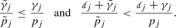
 satisfying
Furthermore, assume that \(q \le {\tilde{q}}\) and that  . Then

Proof
This is an immediate consequence of inequality of Plancherel–Pólya–Nikol’skii type given in Lemma 5.2. \(\square \)
Lemma 5.2
Let X be a Banach space, \({\varvec{p}},\tilde{{\varvec{p}}} \in (1,\infty )^{l}\), and  . Suppose that \(J \subset \{1,\ldots ,l\}\) is such that
\(p_{j} = {\tilde{p}}_{j}\) and \(w_{j} = {\tilde{w}}_{j}\) for \(j \notin J\);
\(w_{j}(x_{j}) = |x_{j}|^{\gamma _{j}}\) and \({\tilde{w}}_{j}(x_{j}) = |x_{j}|^{{\tilde{\gamma }}_{j}}\) for \(j \in J\) for some
 satisfying
 satisfying
Then, there exists a constant \(C>0\) such that, for all \(f \in {\mathcal {S}}'(\mathbb {R}^{d};X)\) with  for some \(R_{1},\ldots ,R_{l} > 0\), we have the inequality

where  for each \(j \in J\).
Proof
Step I.The case\(l=1\):
We refer to [49, Proposition 4.1].
Step II.The case\(J=\{l\}\):
Under the canonical isomorphism  (Schwartz kernel theorem), f corresponds to an element of
  having compact Fourier support contained in
  . Given a compact subset
  we have the continuous linear operator

where  , \({\varvec{p}}':=(p_{1},\ldots ,p_{l-1})\), and \({\varvec{w}}'=(w_{1},\ldots ,w_{l-1})\). Accordingly, for each compact \(K \subset \mathbb {R}^{d'}\) we have
  with compact Fourier support contained in
  , so that we may apply Step I to obtain that

for some constant \(C>0\) independent of f and K. Since  and
and  , the desired result follows by taking
  and letting \(n \rightarrow \infty \).
Step III.The case\(\#J=1\):
Let us say that \(J=\{j_{0}\}\). Then, as a consequence of the Banach space-valued Paley–Wiener–Schwartz theorem, for each fixed  we have that \(f(\cdot ,x'')\) defines an X-valued tempered distribution having compact Fourier support contained in
  . The desired inequality follows by applying Step II to \(f(\cdot ,x'')\) for each \(x''\) and subsequently taking
  -norms with respect to \(x''\).
Step IV. The general case:
Just apply Step III repeatedly (\(\#J\) times). \(\square \)
6 Proof of the main result
In this section, we prove the main result of this paper, Theorem 3.4.
6.1 Necessary conditions on the initial-boundary data
Let the notations and assumptions be as in Theorem 3.4. Suppose that \(g=({\mathcal {B}}_{1}(D)u,\ldots ,{\mathcal {B}}_{n}(D)u)\) and \(u_{0} = \mathrm {tr}_{t=0}u\) for some \(u \in \mathbb {U}^{p,q}_{\gamma ,\mu }\). We show that \((g,u_{0}) \in \mathbb {D}^{p,q}_{\gamma ,\mu }\).
It follows from [50, Theorem 1.1] (also see [55, Theorem 3.4.8]) that
Using standard techniques, one can derive the same result with \(\mathbb {R}\) replaced by J and \(\mathbb {R}^{d}\) replaced by \({\mathscr {O}}\):
In particular, we must have \(u_{0} \in \mathbb {I}^{p,q}_{\gamma ,\mu } \).
In order to show that \(g = (g_{1},\ldots ,g_{n}) \in \mathbb {G}^{p,q}_{\gamma ,\mu }\), we claim that
Combining the fact that
is a \(\left( (d,1),(\frac{1}{2n},1)\right) \)-admissible Banach space (cf. (6)) with (13), (15) and standard techniques of localization, we find
From Theorem 4.4, it thus follows that, for each \(\beta \in \mathbb {N}^{d}\), \(j \in \{1,\ldots ,n\}\) with \(|\beta | \le n_{j}\), \(\mathrm {tr}_{\partial {\mathscr {O}}} \circ D^{\beta }_{x}\) is continuous linear operator
The regularity assumption \((\mathrm {SB})\) on the coefficients \(b_{j,\beta }\) thus gives (39), where we use Lemmas B.1, B.3 and B.4 for \(|\beta |=n_{j}\) and Lemma B.5 for \(|\beta _{j}|<n_{j}\).
Finally, suppose that \(\kappa _{j,\gamma } > \frac{1+\mu }{q}\). Then, by combination of (38), (39) and Remark 3.5,
By a density argument these operators coincide. Hence,
6.2 Elliptic boundary value model problems
Let X be a UMD Banach space. Let \({\mathcal {A}}(D) = \sum _{|\alpha | = 2n}a_{\alpha }D^{\alpha }\)\({\mathcal {B}}_{j}(D) = \sum _{|\beta | =}{ n_{j}}b_{j,\beta }\mathrm {tr}_{\partial \mathbb {R}^{d}_{+}}D^{\beta }\), \(j=1,\ldots ,n\) with constant coefficients \(a_{\alpha },b_{\beta ,j} \in {\mathcal {B}}(X)\).
In this subsection, we study the elliptic boundary value problem
on \(\mathbb {R}^{d}_{+}\). By the trace result of Corollary 4.3, in order to get a solution \(v \in W^{2n}_{p}(\mathbb {R}^{d}_{+},w_{\gamma };X)\) we need \(g=(g_{1},\ldots ,g_{n}) \in \prod _{j=1}^{n}F_{p,p}^{2n\kappa _{j,\gamma }}(\mathbb {R}^{d-1};X)\). In Proposition 6.2, we will see that there is existence and uniqueness plus a certain representation for the solution (which we will use to solve (49)). In this representation, we have the operator from the following lemma.
Lemma 6.1
Let E be a UMD Banach space, let \(p \in (1,\infty )\), \(w \in A_{p}(\mathbb {R}^{d})\), and \(n \in \mathbb {Z}_{>0}\). For each \(\lambda \in \mathbb {C}{\setminus } (-\infty ,0]\) and \(\sigma \in \mathbb {R}\), we define \(L^{\sigma }_{\lambda } \in {\mathcal {L}}({\mathcal {S}}'(\mathbb {R}^{d};E))\) by
Then, \(L^{\sigma }_{\lambda }\) restricts to a topological linear isomorphism from \(H^{s+2n\sigma }_{p}(\mathbb {R}^{d},w;E)\) to \(H^{s}_{p}(\mathbb {R}^{d},w;E)\) (with inverse \(L^{-\sigma }_{\lambda }\)) for each \(s \in \mathbb {R}\). Moreover,
defines an analytic mapping for every \(\sigma \in \mathbb {R}\) and \(s \in \mathbb {R}\).
Proof
For the first part, one only needs to check the Mikhlin condition corresponding to (6) (with \(l=1\) and \({\varvec{a}}=1\)) for the symbol \(\xi \mapsto (1+|\xi |^{2})^{-(n\sigma )/2}(\lambda +|\xi |^{2n})^{\sigma }\). So let us go to the analyticity statement. We only treat the case \(\sigma \in \mathbb {R}{\setminus } \mathbb {N}\), the case \(\sigma \in \mathbb {N}\) being easy. So suppose that \(\sigma \in \mathbb {R}{\setminus } \mathbb {N}\) and fix a \(\lambda _{0} \in \mathbb {C}{\setminus } (-\infty ,0]\). We shall show that \(\lambda \mapsto L^{\sigma }_{\lambda }\) is analytic at \(\lambda _{0}\). Since \(L^{\tau }_{\lambda _{0}}\) is a topological linear isomorphism from \(H^{s+2n\tau }_{p}(\mathbb {R}^{d},w;E)\) to \(H^{s}_{p}(\mathbb {R}^{d},w;E)\), \(\tau \in \mathbb {R}\), for this it suffices to show that
is analytic at \(\lambda _{0}\). To this end, we first observe that, for each \(\xi \in \mathbb {R}^{d}\),
is an analytic mapping with power series expansion at \(\lambda _{0}\) given by
for \(\lambda \in B(\lambda _{0},\delta )\), where \(\delta := d\left( 0,\{\lambda _{0}+t \mid t \ge 0\}\right) > 0\). We next recall that \(L_{\lambda _{0}}^{-1}\) restricts to a topological linear isomorphism from \(L^{p}(\mathbb {R}^{d},w;E)\) to \(H^{2n}_{p}(\mathbb {R}^{d},w;E)\); in particular, \(L_{\lambda _{0}}^{-1}\) restricts to a bounded linear operator on \(L^{p}(\mathbb {R}^{d},w;E)\). Since \(L_{\lambda _{0}}^{-k} = (L_{\lambda _{0}}^{-1})^{k}\) for every \(k \in \mathbb {N}\), there thus exists a constant \(C > 0\) such that
Now we let \(\rho > 0\) be the radius of convergence of the power series \(z \mapsto \sum _{k \in \mathbb {N}}\left[ \prod _{j=0}^{k-1}(\sigma -j)\right] C^{k}z^{k}\), set \(r:= \min (\delta ,\rho ) > 0\), and define, for each \(\lambda \in B(\lambda _{0},r)\), the multiplier symbols \(m^{\lambda },m^{\lambda }_{0},m^{\lambda }_{1},\ldots :\mathbb {R}^{d} \longrightarrow \mathbb {C}\) by
Then, by (42) and (43), we get
and
respectively. Via the \(A_{p}\)-weighted version of [39, Facts 3.3.b], we thus obtain that
for \(\lambda \in B(\lambda _{0},r)\). This shows that the map \(\mathbb {C}{\setminus } (-\infty ,0] \ni \lambda \mapsto L^{\sigma }_{\lambda }L^{-\sigma }_{\lambda _{0}} \in {\mathcal {B}}(L^{p}(\mathbb {R}^{d},w;E))\) is analytic at \(\lambda _{0}\), as desired. \(\square \)
Before we can state Proposition 6.2, we first need to introduce some notation. Given a UMD Banach space X and a natural number \(k \in \mathbb {N}\), we have, for the UMD space \(E=L^{p}(\mathbb {R}_{+},|\,\cdot \,|^{\gamma };X)\), the natural inclusion
and the natural identification
By Lemma 6.1, we accordingly have that, for \(\lambda \in \mathbb {C}{\setminus } (-\infty ,0]\), that the partial Fourier multiplier operator
restricts to a bounded linear operator
Moreover, we even get an analytic operator-valued mapping
In particular, we have
with analytic dependence on the parameter \(\lambda \in \mathbb {C}{\setminus } (-\infty ,0]\).
Proposition 6.2
Let X be a UMD Banach space, \(p \in (1,\infty )\), \(\gamma \in (-1,p-1)\), and assume that \(({\mathcal {A}},{\mathcal {B}}_{1},\ldots ,{\mathcal {B}}_{n})\) satisfies \((\mathrm {E})\) and \((\mathrm {LS})\) for some \(\phi \in (0,\pi )\). Then, for each \(\lambda \in \Sigma _{\pi -\phi }\), there exists an operator
which assigns to a \(g \in \bigoplus _{j=1}^{n}F_{p,p}^{2n\kappa _{j,\gamma }}(\mathbb {R}^{d-1};X)\) the unique solution \(v={\mathcal {S}}(\lambda )g \in W^{2n}_{p}(\mathbb {R}^{d}_{+},w_{\gamma };X)\) of the elliptic boundary value problem
recall here that \(\kappa _{j,\gamma } = 1-\frac{n_{j}}{2n}-\frac{1}{2np}(1+\gamma )\). Moreover, for each \(j \in \{1,\ldots ,n\}\), we have that
defines an analytic mapping, for which the operators \(D^{\alpha }\tilde{{\mathcal {S}}}_{j}(\lambda ) \in {\mathcal {B}}(W^{2n-n_{j}}_{p}(\mathbb {R}^{d}_{+},w_{\gamma };X),L^{p}(\mathbb {R}^{d}_{+},w_{\gamma };X))\), \(|\alpha | \le 2n\), can be represented as
for analytic operator-valued mappings
satisfying the \({\mathcal {R}}\)-bounds
Comments on the proof of Proposition 6.2
This proposition can be proved in the same way as [18, Lemma 4.3 & Lemma 4.4]. In fact, in the unweighted case this is just a modification of [18, Lemma 4.3 & Lemma 4.4] (also see the formulation of [47, Lemma 2.2.6]). Here, [18, Lemma 4.3] corresponds to the existence of the solution operator, whose construction was essentially already contained in [17], plus its representation, and [18, Lemma 4.4] basically corresponds to the analytic dependence of (47) plus the \({\mathcal {R}}\)-bounds (48). The analytic dependence of the operators \(\tilde{{\mathcal {S}}}_{j}(\lambda )\) on \(\lambda \) subsequently follows from Lemma 6.1 and (46). For more details, we refer to [42, Chapter 6] and Remark 6.4. \(\square \)
Remark 6.3
We could have formulated Proposition 6.2 only in terms of the mappings \(\tilde{{\mathcal {S}}}_{j}\). Namely, for each \(j \in \{1,\ldots ,n\}\) there exists an analytic mapping
with the property that, for every \(u \in W^{2n}_{p}(\mathbb {R}^{d}_{+},w_{\gamma };X)\), \(v = \tilde{{\mathcal {S}}}_{j}u\) is the unique solution in \(W^{2n}_{p}(\mathbb {R}^{d}_{+},w_{\gamma };X)\) of (45) with \(g_{i}=\delta _{i,j}{\mathcal {B}}_{i}(D)u\), for which the operators
can be represented as (46) for analytic operator-valued mappings (47) satisfying the \({\mathcal {R}}\)-bounds (48). Then, given extension operators \({\mathcal {E}}_{j} \in {\mathcal {B}}(F^{2n\kappa _{j,\gamma }}_{p,p}(\mathbb {R}^{d-1};X),W^{2n-n_{j}}_{p}(\mathbb {R}^{d}_{+},w_{\gamma };X))\) (right inverse of the trace \(\mathrm {tr}_{y=0} \in {\mathcal {B}}(W^{2n-n_{j}}_{p}(\mathbb {R}^{d}_{+},w_{\gamma };X),F^{2n\kappa _{j,\gamma }}_{p,p}(\mathbb {R}^{d-1};X))\)), \(j=1,\ldots ,n\), the composition \({\mathcal {S}}(\lambda ) = ( {\mathcal {S}}_{1}(\lambda ) \ldots {\mathcal {S}}_{n}(\lambda ) ) := ( {\mathcal {S}}_{1}(\lambda ) \ldots {\mathcal {S}}_{n}(\lambda ) ) \circ ({\mathcal {E}}_{1} \ldots {\mathcal {E}}_{n})\) defines the desired solution operator.
In this formulation, the proposition the weight \(w_{\gamma }\) can actually be replaced by any weight w on \(\mathbb {R}^{d}\) which is uniformly \(A_{p}\) in the y-variable. Indeed, in the proof the weight only comes into play in [17, Lemma 7.1]. For weights w of the form \(w(x',y) = v(x')|y|^{\gamma }\) with \(v \in A_{p}(\mathbb {R}^{d-1})\), we can then still define \({\mathcal {S}}(\lambda )\) as above thanks to the available trace theory from Sect. 4.1.
Remark 6.4
In [18] the specific extension operator \({\mathcal {E}}_{\lambda } = e^{-\,\cdot \,L^{1/2n}_{\lambda }}\) was used in the construction of the solution operator \({\mathcal {S}}(\lambda ) = ({\mathcal {S}}_{1}(\lambda ),\ldots ,{\mathcal {S}}_{n}(\lambda ))\), which has the advantageous property that \(D_{y}{\mathcal {E}}_{\lambda } = \imath L_{\lambda }^{1/2n}{\mathcal {E}}_{\lambda }\). Whereas in this way the obtained representation formulae \({\mathcal {S}}_{j}(\lambda ) = {\mathcal {T}}_{j}(\lambda )L_{\lambda }^{1-\frac{n_{j}}{2n}}{\mathcal {E}}_{\lambda }\) can only be used in the case \(q=p\) to solve (49) via a Fourier transformation in time (cf. [18, Proposition 4.5] and [47, Lemma 2.2.7]), our representation formulae (46) can (in combination with the theory of anisotropic function spaces) be used to solve (49) in the full parameter range \(q,p \in (1,\infty )\) (cf. Corollary 6.8). However, the alternative more involved proof of Denk, Hieber & Prüss [18, Theorem 2.3] also contains several ingredients which are of independent interest.
6.3 Solving inhomogeneous boundary data for a model problem
Let the notations and assumptions be as in Theorem 3.4, but for the model problem case of top-order constant coefficients on the half-space considered in Sect. 6.2.
The goal of this subsection is to solve the model problem
for \(g=(g_{1},\ldots ,g_{n})\) with \((0,g,0) \in \mathbb {D}^{p,q}_{\gamma ,\mu }\).
Let us first observe that, in view of the compatibility condition in the definition of \(\mathbb {D}^{p,q}_{\gamma ,\mu }\), \((0,g,0) \in \mathbb {D}^{p,q}_{\gamma ,\mu }\) if and only if
for all \(j \in \{1,\ldots ,n\}\). Defining
we thus have \((0,g,0) \in \mathbb {D}^{p,q}_{\gamma ,\mu }\) if and only if \(g \in {_{0}}\mathbb {G}\). So we need to solve (49) for \(g \in {_{0}}\mathbb {G}\).
We will solve (49) by passing to the corresponding problem on \(\mathbb {R}\) (instead of \(\mathbb {R}_{+}\)). The advantage of this is that it allows us to use the Fourier transform in time. This will give
where \({\mathcal {S}}(1+\imath \theta )\) is the solution operator from Proposition 6.2.
Recall that for the operator \(\tilde{{\mathcal {S}}}_{j}(\lambda ) = {\mathcal {S}}_{j}(\lambda ) \circ \mathrm {tr}_{y=0}\) we have the representation formula (46) in which the operators \(L^{\sigma }_{\lambda }\) occur. It will be useful to note that, for \(h \in {\mathcal {S}}(\mathbb {R}^{d}_{+} \times \mathbb {R};X)\),
where
Lemma 6.5
Let E be a UMD space, \(p,q \in (1,\infty )\), \(v \in A_{q}(\mathbb {R})\), and \(n \in \mathbb {Z}_{>0}\). For each \(\sigma \in \mathbb {R}\),
restricts to a bounded linear operator
Proof
This can be shown by checking that the symbol
satisfies the anisotropic Mikhlin condition from (6). \(\square \)
Lemma 6.6
Let X be a UMD space, \(q,p \in (1,\infty )\), \(\gamma \in (-1,p-1)\), \(v \in A_{q}(\mathbb {R})\). Put
where we recall that \(\kappa _{j,\gamma } = 1-\frac{n_{j}}{2n}-\frac{1}{2np}(1+\gamma ) \in (0,1)\). Furthermore, define \({_{0}}{\overline{\mathbb {G}}}_{j}\) similarly to \({_{0}}\mathbb {G}_{j}\) and put \({_{0}}{\overline{\mathbb {G}}}_{j} := {_{0}}{\overline{\mathbb {G}}}_{1} \oplus \ldots \oplus {_{0}}{\overline{\mathbb {G}}}_{n}\). Then the problem
admits a bounded linear solution operator \(\overline{{\mathscr {S}}} : {\overline{\mathbb {G}}} \longrightarrow {\overline{\mathbb {U}}}\) which maps \({_{0}}{\overline{\mathbb {G}}}\) to \({_{0}}{\overline{\mathbb {U}}} = \{ u \in {\overline{\mathbb {U}}} : u(0)=0 \}\).
For the statement that \(\overline{{\mathscr {S}}}\) maps \({_{0}}{\overline{\mathbb {G}}}\) to \({_{0}}{\overline{\mathbb {U}}}\), we will use the following lemma.
Lemma 6.7
\(\{g_{j} \in {\mathcal {S}}(\mathbb {R}^{d};X) : \mathrm {tr}_{t=0}g_{j}=0\}\) is dense in \({_{0}}{\overline{\mathbb {G}}}_{j}\)
Proof
As a consequence of Theorem 2.1,
where
Let \((S_{n})_{n \in \mathbb {N}}\) be the family of convolution operator corresponding to some \(\varphi = (\varphi _{n})_{n \in \mathbb {N}} \in \Phi (\mathbb {R}^{d-1})\). Then, \(S_{n} {\mathop {\longrightarrow }\limits ^{\mathrm {SOT}}} I\) as \(n \rightarrow \infty \) in both \(L^{p}(\mathbb {R}^{d-1};X)\) as \(F^{2n\kappa _{j,\gamma }}_{p,p}(\mathbb {R}^{d-1};X)\). For the pointwise induced operator family, we thus have \(S_{n} {\mathop {\longrightarrow }\limits ^{\mathrm {SOT}}} I\) in \({_{0}}{\overline{\mathbb {G}}}_{j}\). Since
it follows that
is dense in \({_{0}}{\overline{\mathbb {G}}}_{j}\); in fact,
Since
by [44], the desired density follows. \(\square \)
Proof of Lemma 6.6
(I) Put \({\overline{\mathbb {F}}}:= L^{q}(\mathbb {R},v;L^{p}(\mathbb {R}^{d}_{+},w_{\gamma };X))\) and \(V:= {\mathscr {F}}^{-1}C^{\infty }_{c}(\mathbb {R}^{d-1};X) \otimes {\mathscr {F}}^{-1}C^{\infty }_{c}(\mathbb {R})\). Then \(V^{n}\) is dense in \({\overline{\mathbb {G}}}\). So, in view of
it suffices to construct a solution operator \(\overline{{\mathscr {S}}}:V^{n} \longrightarrow {\overline{\mathbb {U}}}\) which is bounded when \(V^{n}\) carries the induced norm from \({\overline{\mathbb {G}}}\). In order to define such an operator, fix \(g=(g_{1},\ldots ,g_{n}) \in V^{n}\). Let
be extension operators (right inverses of the trace operator \(\mathrm {tr}_{y=0}\)) as in Corollary 4.9. Then, \({\mathcal {E}}_{j}\) maps \(V^{n}\) into \({\mathcal {S}}(\mathbb {R}^{d}_{+};X)) \otimes {\mathscr {F}}^{-1}(C^{\infty }_{c}(\mathbb {R}))\); in particular,
So, for each \(j \in \{1,\ldots ,n\}\), we have
and we may also view \({\mathscr {F}}_{t}{\mathcal {E}}_{j}g_{j}\) as a function
Since
with \(\tilde{{\mathcal {S}}}_{j}(1+\imath \theta )\) as in Proposition 6.2, we may thus define
(II) We now show that \(u=\overline{{\mathscr {S}}}g \in {\mathcal {S}}(\mathbb {R};W^{2n}_{p}(\mathbb {R}^{d}_{+},w_{\gamma };X))\) is a solution of (52) for \(g \in V^{n}\). To this end, let \(\theta \in \mathbb {R}\) be arbitrary. Then, we have that \(({\mathscr {F}}_{t}{\mathcal {E}}_{j}g_{j})(\theta ) \in {\mathcal {S}}(\mathbb {R}^{d}_{+};X) \subset W^{2n-n_{j}}_{p}(\mathbb {R}^{d}_{+},w_{\gamma };X)\) and \(({\mathscr {F}}_{t}g_{j})(\theta ) \in {\mathcal {S}}(\mathbb {R}^{d-1};X) \subset F^{2n\kappa _{j,\gamma }}_{p,p}(\mathbb {R}^{d-1};X)\) are related by \(\mathrm {tr}_{y=0}({\mathscr {F}}_{t}{\mathcal {E}}_{j}g_{j})(\theta ) = ({\mathscr {F}}_{t}g_{j})(\theta )\); just note that \(({\mathscr {F}}_{t}{\mathcal {E}}_{j}g_{j})(0,x',\theta ) = ({\mathscr {F}}_{t}g_{j})(x',\theta )\) for every \(x' \in \mathbb {R}^{d-1}\). Therefore, by Proposition 6.2, \(v(\theta ) = ({\mathscr {F}}_{t}u)(\theta ) =({\mathscr {F}}_{t}\overline{{\mathscr {S}}}g)(\theta ) = \sum _{j=1}^{n}\tilde{{\mathcal {S}}}_{j}(1+\imath \theta ) ({\mathscr {F}}_{t}{\mathcal {E}}_{j}g_{j})(\theta ) \in W^{2n}_{p}(\mathbb {R}^{d}_{+},w_{\gamma };X)\) is the unique solution of the problem
Applying the inverse Fourier transform \({\mathscr {F}}_{t}^{-1}\) with respect to \(\theta \), we find
(III) We next derive a representation formula for \(\overline{{\mathscr {S}}}\) that is well suited for proving the boundedness of \(\overline{{\mathscr {S}}}\). To this end, fix a \(g=(g_{1},\ldots ,g_{n}) \in V^{n}\). Then we have, for each multi-index \(\alpha \in \mathbb {N}^{d}, |\alpha | \le 2n\),
(IV) We next show that \(||\overline{{\mathscr {S}}}g||_{{\overline{\mathbb {U}}}} \lesssim ||g||_{{\overline{\mathbb {G}}}}\) for \(g \in V^{n}\). Being a solution of (52), \(\overline{{\mathscr {S}}}g\) satisfies
Hence, it suffices to establish the estimate \(||D^{\alpha }\overline{{\mathscr {S}}}g||_{{\overline{\mathbb {F}}}} \lesssim ||g||_{{\overline{\mathbb {G}}}}\) for all multi-indices \(\alpha \in \mathbb {N}^{d}, |\alpha | \le 2n\). So fix such an \(|\alpha | \le 2n\). Then, in view of the representation formula (54), it is enough to show that
and
We only treat estimate (56), estimate (55) being similar (but easier): Fix a \(j \in \{1,\ldots ,n\}\). For the full \((d+1)\)-dimensional Euclidean space \(\mathbb {R}^{d} \times \mathbb {R}\) instead of \(\mathbb {R}^{d}_{+} \times \mathbb {R}\),
follows from (15) (and the fact that \(L_{(p,q),(d,1)}(\mathbb {R}^{d+1},(w_{\gamma },v_{\mu });X)\) is an admissible Banach space of X-valued tempered distributions on \(\mathbb {R}^{d+1}\) in view of (6)), from which the \(\mathbb {R}^{d}_{+} \times \mathbb {R}\)-case follows by restriction. In combination with (53) and Lemma 6.5, this yields
Furthermore, we have that \({\mathcal {T}}^{2}_{j,\alpha }(1+\imath \cdot ) \in C^{\infty }(\mathbb {R};{\mathcal {B}}(L^{p}(\mathbb {R}^{d}_{+},w_{\gamma };X)))\) satisfies
by the Kahane contraction principle and (48); in particular, \({\mathcal {T}}^{2}_{j,\alpha }(1+\imath \cdot )\) satisfies the Mikhlin condition corresponding to (7). As a consequence, \({\mathcal {T}}^{2}_{j,\alpha }(1+\imath \cdot )\) defines a bounded Fourier multiplier operator on \(L^{q}(\mathbb {R},v;L^{p}(\mathbb {R}^{d}_{+},w_{\gamma };X))\). In combination with (57), this gives estimate (56).
(V) We finally show that \(\overline{{\mathscr {S}}} \in {\mathcal {B}}({\overline{\mathbb {G}}},{\overline{\mathbb {U}}})\) maps \({_{0}}{\overline{\mathbb {G}}}\) to \({_{0}}{\overline{\mathbb {U}}}\). As in the proof of [47, Lemma 2.2.7], it can be shown that, if
and
satisfy (52), then \(u(0)=0\). The desired statement thus follows from Lemma 6.7. \(\square \)
Corollary 6.8
Let the notations and assumptions be as in Theorem 3.4, but for the model problem case of top-order constant coefficients on the half-space considered in Sect. 6.2. Then, problem (49) admits a bounded linear solution operator
6.4 Proof of Theorem 3.4
We can now finally prove the main result of this paper.
Proof of Theorem 3.4
In view of Sect. 6.1, it remains to establish existence and uniqueness of a solution \(u \in \mathbb {U}^{p,q}_{\gamma ,\mu }\) of (20) for given \((f,g,u_{0}) \in \mathbb {G}^{p,q}_{\gamma ,\mu } \oplus \mathbb {D}^{p,q}_{\gamma ,\mu }\). By a standard (but quite technical) perturbation and localization procedure, it is enough to consider the model problem
on the half-space, where \({\mathcal {A}}\) and \({\mathcal {B}}_{1},\ldots ,{\mathcal {B}}_{n}\) are top-order constant coefficient operators as considered in Sect. 6.2. This procedure is worked out in full detail in [47]; for further comments we refer to “Appendix 7.”
Let \((f,g,u_{0}) \in \mathbb {F}^{p,q}_{\gamma ,\mu } \oplus \mathbb {D}^{p,q}_{\gamma ,\mu }\). In view of Theorem 4.4 and the fact that \(\mathrm {tr}_{t=0} \circ {\mathcal {B}}_{j}(D) = {\mathcal {B}}_{j}(D)\) on \(\mathbb {U}^{p,q}_{\gamma ,\mu } \circ \mathrm {tr}_{t=0}\) when \(\kappa _{j,\gamma } < \frac{1+\mu }{q}\), we may without loss of generality assume that \(u_{0}=0\). By Corollary 6.8 we may furthermore assume that \(g=0\). Defining \(A_{B}\) as the operator on \(Y = L^{p}(\mathbb {R}^{d}_{+},w_{\gamma })\) with domain
and given by the rule \(A_{B}v :={\mathcal {A}}(D)v\), we need to show that \(1+A_{B}\) enjoys the property of maximal \(L^{q}_{\mu }\)-regularity: for every \(f \in L^{q}(\mathbb {R}_{+},v_{\mu };Y)\) there exists a unique \(u \in {_{0}}W^{1}_{q}(\mathbb {R}_{+},v_{\mu };Y) \cap L^{q}(\mathbb {R}_{+},v_{\mu };D(A_{B}))\) with \(u'+(1+A_{B})u=f\). In the same way as in [17, Theorem 7.4] it can be shown that \(A_{B} \in {\mathcal {H}}^{\infty }(Y)\) with angle \(\phi ^{\infty }_{A_{B}} < \frac{\pi }{2}\). As Y is a UMD space, \(1+A_{B}\) enjoys maximal \(L^{q}_{\mu }\)-regularity for \(\mu =0\); see, e.g., [66, Section 4.4] and the references therein. By [12, 54] this extrapolates to all \(\mu \in (-1,q-1)\) (i.e., all \(\mu \) for which \(v_{\mu } \in A_{q}\)). \(\square \)
Notes
This technical condition on \({\varvec{w}}''\) is in particular satisfied when \({\varvec{p}}'' \in (1,\infty )^{l-1}\) and
 .
.
 .
.References
P. Acquistapace and B. Terreni. A unified approach to abstract linear nonautonomous parabolic equations. Rend. Sem. Mat. Univ. Padova, 78:47–107, 1987.
E. Alòs and S. Bonaccorsi. Stability for stochastic partial differential equations with Dirichlet white-noise boundary conditions. Infin. Dimens. Anal. Quantum Probab. Relat. Top., 5(4):465–481, 2002.
H. Amann. Linear and quasilinear parabolic problems. Vol. I, volume 89 of Monographs in Mathematics. Birkhäuser Boston, Inc., Boston, MA, 1995. Abstract linear theory.
H. Amann. Vector-Valued Distributions and Fourier Multipliers. Unpublished notes, 2003.
H. Amann. Maximal regularity and quasilinear parabolic boundary value problems. In Recent advances in elliptic and parabolic problems, pages 1–17. World Sci. Publ., Hackensack, NJ, 2005.
H. Amann. Anisotropic function spaces and maximal regularity for parabolic problems. Part 1. Jindr̆ich Nec̆as Center for Mathematical Modeling Lecture Notes, 6. Matfyzpress, Prague, 2009.
S.B. Angenent. Nonlinear analytic semiflows. Proc. Roy. Soc. Edinburgh Sect. A, 115(1-2):91–107, 1990.
J. Bourgain. Vector-valued singular integrals and the \(H^1\)-BMO duality. In Probability theory and harmonic analysis (Cleveland, Ohio, 1983), volume 98 of Monogr. Textbooks Pure Appl. Math., pages 1–19. Dekker, New York, 1986.
K. Brewster and M. Mitrea. Boundary value problems in weighted Sobolev spaces on Lipschitz manifolds. Mem. Differ. Equ. Math. Phys., 60:15–55, 2013.
Z. Brzeźniak, B. Goldys, S. Peszat, and F. Russo. Second order PDEs with Dirichlet white noise boundary conditions. J. Evol. Equ., 15(1):1–26, 2015.
H-Q Bui. Weighted Besov and Triebel spaces: interpolation by the real method. Hiroshima Math. J., 12(3):581–605, 1982.
R. Chill and A. Fiorenza. Singular integral operators with operator-valued kernels, and extrapolation of maximal regularity into rearrangement invariant Banach function spaces. J. Evol. Equ., 14(4-5):795–828, 2014.
P. Clément and S. Li. Abstract parabolic quasilinear equations and application to a groundwater flow problem. Adv. Math. Sci. Appl., 3(Special Issue):17–32, 1993/94.
P. Clément and J. Prüss. Global existence for a semilinear parabolic Volterra equation. Math. Z., 209(1):17–26, 1992.
P. Clément and G. Simonett. Maximal regularity in continuous interpolation spaces and quasilinear parabolic equations. J. Evol. Equ., 1(1):39–67, 2001.
G. Da Prato and P. Grisvard. Sommes d’opérateurs linéaires et équations différentielles opérationnelles. J. Math. Pures Appl. (9), 54(3):305–387, 1975.
R. Denk, M. Hieber, and J. Prüss. \({\cal{R}}\)-boundedness, Fourier multipliers and problems of elliptic and parabolic type. Mem. Amer. Math. Soc., 166(788):viii+114, 2003.
R. Denk, M. Hieber, and J. Prüss. Optimal \(L^p\)-\(L^q\)-estimates for parabolic boundary value problems with inhomogeneous data. Math. Z., 257(1):193–224, 2007.
R. Denk and M. Kaip. General parabolic mixed order systems in \({L_p}\)and applications, volume 239 of Operator Theory: Advances and Applications. Birkhäuser/Springer, Cham, 2013.
R. Denk, J. Prüss, and R. Zacher. Maximal \(L_p\)-regularity of parabolic problems with boundary dynamics of relaxation type. J. Funct. Anal., 255(11):3149–3187, 2008.
R. Denk, J. Saal, and J. Seiler. Inhomogeneous symbols, the Newton polygon, and maximal \(L^p\)-regularity. Russ. J. Math. Phys., 15(2):171–191, 2008.
R. Denk and R. Schnaubelt. A structurally damped plate equation with Dirichlet–Neumann boundary conditions. J. Differential Equations, 259(4):1323–1353, 2015.
G. Dore and A. Venni. On the closedness of the sum of two closed operators. Math. Z., 196(2):189–201, 1987.
J. Escher, J. Prüss, and G. Simonett. Analytic solutions for a Stefan problem with Gibbs–Thomson correction. J. Reine Angew. Math., 563:1–52, 2003.
G. Fabbri and B. Goldys. An LQ problem for the heat equation on the halfline with Dirichlet boundary control and noise. SIAM J. Control Optim., 48(3):1473–1488, 2009.
S. Fackler, T.P. Hytönen, and N. Lindemulder. Weighted Estimates for Operator-Valued Fourier Multipliers. arXiv e-prints, page arXiv:1810.00172, Sep 2018.
R. Farwig and H. Sohr. Weighted \(L^q\)-theory for the Stokes resolvent in exterior domains. J. Math. Soc. Japan, 49(2):251–288, 1997.
C. Gallarati, E. Lorist, and M.C. Veraar. On the \(\ell ^s\)-boundedness of a family of integral operators. Rev. Mat. Iberoam., 32(4):1277–1294, 2016.
J. García-Cuerva, R. Macías, and J. L. Torrea. The Hardy–Littlewood property of Banach lattices. Israel J. Math., 83(1-2):177–201, 1993.
Y. Giga. Solutions for semilinear parabolic equations in \(L^p\) and regularity of weak solutions of the Navier–Stokes system. J. Differential Equations, 62(2):186–212, 1986.
L. Grafakos. Modern Fourier analysis, volume 250 of Graduate Texts in Mathematics. Springer, New York, second edition, 2009.
D.D. Haroske and L. Skrzypczak. Entropy and approximation numbers of embeddings of function spaces with Muckenhoupt weights, II. General weights. Ann. Acad. Sci. Fenn. Math., 36(1):111–138, 2011.
T.P. Hytönen, J.M.A.M. van Neerven, M.C. Veraar, and L. Weis. Analysis in Banach spaces. Volume I. Martingales and Littlewood–Paley theory. Ergebnisse der Mathematik und ihrer Grenzgebiete, Springer-Verlag. 2016.
J. Johnsen. Elliptic boundary problems and the Boutet de Monvel calculus in Besov and Triebel–Lizorkin spaces. Math. Scand., 79(1):25–85, 1996.
J. Johnsen and W. Sickel. A direct proof of Sobolev embeddings for quasi-homogeneous Lizorkin–Triebel spaces with mixed norms. J. Funct. Spaces Appl., 5(2):183–198, 2007.
J. Johnsen and W. Sickel. On the trace problem for Lizorkin–Triebel spaces with mixed norms. Math. Nachr., 281(5):669–696, 2008.
N. J. Kalton and L. Weis. The \(H^\infty \)-calculus and sums of closed operators. Math. Ann., 321(2):319–345, 2001.
M. Köhne, J. Prüss, and M. Wilke. On quasilinear parabolic evolution equations in weighted \(L_p\)-spaces. J. Evol. Equ., 10(2):443–463, 2010.
P.C. Kunstmann and L. Weis. Maximal \(L_p\)-regularity for parabolic equations, Fourier multiplier theorems and \(H^\infty \)-functional calculus. In Functional analytic methods for evolution equations, volume 1855 of Lecture Notes in Math., pages 65–311. Springer, Berlin, 2004.
O. A. Ladyženskaja, V. A. Solonnikov, and N. N. Ural’ceva. Linear and quasilinear equations of parabolic type. Translated from the Russian by S. Smith. Translations of Mathematical Monographs, Vol. 23. American Mathematical Society, Providence, R.I., 1968.
J. LeCrone, J. Pruess, and M. Wilke. On quasilinear parabolic evolution equations in weighted \(L_p\)-spaces II. J. Evol. Equ., 14(3):509–533, 2014.
N. Lindemulder. Parabolic Initial-Boundary Value Problems with Inhomogeneous Data: A weighted maximal regularity approach. Master’s thesis, Utrecht University, 2014.
N. Lindemulder. An Intersection Representation for a Class of Vector-valued Anisotropic Function Spaces. ArXiv e-prints (arXiv:1903.02980), March 2019.
N. Lindemulder, M. Meyries, and M.C. Veraar. Interpolation with normal boundary conditions for function spaces with power weights. 2019. In preparation.
A. Lunardi. Analytic semigroups and optimal regularity in parabolic problems. Progress in Nonlinear Differential Equations and their Applications, 16. Birkhäuser Verlag, Basel, 1995.
V. Maz’ya and T. Shaposhnikova. Higher regularity in the layer potential theory for Lipschitz domains. Indiana Univ. Math. J., 54(1):99–142, 2005.
M. Meyries. Maximal regularity in weighted spaces, nonlinear boundary conditions, and global attractors. PhD thesis, Karlsruhe Institute of Technology, 2010.
M. Meyries and R. Schnaubelt. Maximal regularity with temporal weights for parabolic problems with inhomogeneous boundary conditions. Math. Nachr., 285(8-9):1032–1051, 2012.
M. Meyries and M.C Veraar. Sharp embedding results for spaces of smooth functions with power weights. Studia Math., 208(3):257–293, 2012.
M. Meyries and M.C. Veraar. Traces and embeddings of anisotropic function spaces. Math. Ann., 360(3-4):571–606, 2014.
M. Meyries and M.C. Veraar. Pointwise multiplication on vector-valued function spaces with power weights. J. Fourier Anal. Appl., 21(1):95–136, 2015.
M. Mitrea and M. Taylor. The Poisson problem in weighted Sobolev spaces on Lipschitz domains. Indiana Univ. Math. J., 55(3):1063–1089, 2006.
J. Prüss. Maximal regularity for evolution equations in \(L_p\)-spaces. Conf. Semin. Mat. Univ. Bari, (285):1–39 (2003), 2002.
J. Prüss and G. Simonett. Maximal regularity for evolution equations in weighted \(L_p\)-spaces. Arch. Math. (Basel), 82(5):415–431, 2004.
Jan Prüss and Gieri Simonett. Moving interfaces and quasilinear parabolic evolution equations. Basel: Birkhäuser/Springer, 2016.
D. Roberts. Equations with Dirichlet Boundary Noise. PhD thesis, The University of New South Wales, 2011.
J.L. Rubio de Francia. Martingale and integral transforms of Banach space valued functions. In Probability and Banach spaces (Zaragoza, 1985), volume 1221 of Lecture Notes in Math., pages 195–222. Springer, Berlin, 1986.
T. Runst and W. Sickel. Sobolev spaces of fractional order, Nemytskij operators, and nonlinear partial differential equations, volume 3 of de Gruyter Series in Nonlinear Analysis and Applications. Walter de Gruyter & Co., Berlin, 1996.
V.S. Rychkov. On restrictions and extensions of the Besov and Triebel–Lizorkin spaces with respect to Lipschitz domains. J. London Math. Soc. (2), 60(1):237–257, 1999.
B. Scharf, H-J. Schmeißer, and W. Sickel. Traces of vector-valued Sobolev spaces. Math. Nachr., 285(8-9):1082–1106, 2012.
Y. Shibata and S. Shimizu. On the \(L_p\)-\(L_q\) maximal regularity of the Neumann problem for the Stokes equations in a bounded domain. J. Reine Angew. Math., 615:157–209, 2008.
R. B. Sowers. Multidimensional reaction-diffusion equations with white noise boundary perturbations. Ann. Probab., 22(4):2071–2121, 1994.
S.A. Tozoni. Vector-valued extensions of operators on martingales. J. Math. Anal. Appl., 201(1):128–151, 1996.
P. Weidemaier. Maximal regularity for parabolic equations with inhomogeneous boundary conditions in Sobolev spaces with mixed \(L_p\)-norm. Electron. Res. Announc. Amer. Math. Soc., 8:47–51, 2002.
L. Weis. Operator-valued Fourier multiplier theorems and maximal \(L_p\)-regularity. Math. Ann., 319(4):735–758, 2001.
L. Weis. The \(H^\infty \) holomorphic functional calculus for sectorial operators—a survey. In Partial differential equations and functional analysis, volume 168 of Oper. Theory Adv. Appl., pages 263–294. Birkhäuser, Basel, 2006.
Acknowledgements
The author would like to thank Mark Veraar for the supervision of his master thesis [42], which led to the present paper.
Author information
Authors and Affiliations
Corresponding author
Additional information
Publisher's Note
Springer Nature remains neutral with regard to jurisdictional claims in published maps and institutional affiliations.
The author is supported by the Vidi subsidy 639.032.427 of the Netherlands Organisation for Scientific Research (NWO).
Appendices
Appendix A: Series Estimates in Triebel–Lizorkin and Besov Spaces
Lemma A.1
Let X be a Banach space, \({\varvec{a}} \in (0,\infty )^{l}\), \({\varvec{p}} \in [1,\infty )^{l}\), \(q \in [1,\infty ]\), \(s > 0\), and  . Suppose that there exists an \({\varvec{r}} \in (0,1)^{l}\) such that
  and
and  . Then, for every \(c>0\), there exists a constant \(C>0\) such that, for all \((f_{k})_{k \in \mathbb {N}} \subset {\mathcal {S}}'(\mathbb {R}^{d};X)\) satisfying
  and
and

it holds that \(\sum _{k \in \mathbb {N}}f_{k}\) defines a convergent series in \({\mathcal {S}}'(\mathbb {R}^{d};X)\) with limit  of norm
  .
.
Proof
This can be proved in the same way as [36, Lemma 3.19], using Lemma A.5 below instead of [36, Proposition 3.14]. For more details, we refer to [42, Lemma 5.2.22].
\(\square \)
Lemma A.2
Let X be a Banach space, \({\varvec{a}} \in (0,\infty )^{l}\), \({\varvec{p}} \in [1,\infty )^{l}\), \(q \in [1,\infty ]\), \(s \in \mathbb {R}\), and  . For every \(c>1\), there exists a constant \(C>0\) such that, for all \((f_{k})_{k \in \mathbb {N}} \subset {\mathcal {S}}'(\mathbb {R}^{d};X)\) satisfying

and

it holds that \(\sum _{k \in \mathbb {N}}f_{k}\) defines a convergent series in \({\mathcal {S}}'(\mathbb {R}^{d};X)\) with limit  of norm
  .
.
Proof
This can be proved in the same way as [36, Lemma 3.20]. In fact, one only needs a minor modification of the proof of Lemma A.1. \(\square \)
Lemma A.3
Let X be a Banach space, \({\varvec{a}} \in (0,\infty )^{l}\), \({\varvec{p}} \in [1,\infty )^{l}\), \(q \in [1,\infty ]\), \(s \in \mathbb {R}\), and  . For every \(c>1\), there exists a constant \(C>0\) such that, for all \((f_{k})_{k \in \mathbb {N}} \subset {\mathcal {S}}'(\mathbb {R}^{d};X)\) satisfying (58) and

it holds that \(\sum _{k \in \mathbb {N}}f_{k}\) defines a convergent series in \({\mathcal {S}}'(\mathbb {R}^{d};X)\) with limit  of norm
  .
.
The above two lemmas are through Lemma A.5 based on the following maximal inequality:
Lemma A.4
Let \({\varvec{a}} \in (0,\infty )^{l}\) and  . Let \(j_{0} \in \{1,\ldots ,l\}\) and \(r_{j_{0}} \in (0,\min \{p_{j_{0}},\ldots ,p_{l}\})\) be such that
  . Then

gives rise to a well-defined bounded sublinear operator  on
on  . Moreover, there holds a Fefferman–Stein inequality for
  : for every \(q \in (\max \{1,r\},\infty ]\) there exists a constant \(C \in (0,\infty )\) such that, for all sequences
  ,
,

Proof
This can be easily derived from [28, Theorem 2.6], which is a weighted version of the special case of the \(L^{p}\)-boundedness of the Banach lattice version of the Hardy–Littlewood maximal function [8, 29, 57, 63] for mixed-norm spaces (also see [28, Remark 2.7]). \(\square \)
Lemma A.5
Let X be a Banach space, \({\varvec{p}} \in [1,\infty )^{l}\), \(q \in [1,\infty ]\), and  . Suppose \({\varvec{r}} \in (0,1)^{l}\) is such that
  for \(j=1,\ldots ,l\). Let \(\psi \in {\mathcal {S}}(\mathbb {R}^{d})\) be such that
  , and set
  for each \(n \in \mathbb {N}\). Then, there exists a constant \(C>0\) such that, for all \((f_{n})_{n \in \mathbb {N}} \subset {\mathcal {S}}'(\mathbb {R}^{d};X)\) with
  for some \(R \ge 1\), the following inequality holds true:

Proof
As in the proof of [36, Proposition 3.14], it can be shown that

for some constant \(c>0\) independent of \((f_{n})_{n}\). The desired result now follows from Lemma A.4. \(\square \)
Given a function \(f:\mathbb {R}^{d} \longrightarrow X\), \({\varvec{r}} \in (0,\infty )^{l}\) and \({\varvec{b}} \in (0,\infty )^{l}\), we define the maximal function of Peetre–Fefferman–Stein type by
by

Lemma A.6
Let X be a Banach space, \({\varvec{p}} \in [1,\infty )^{l}\), \(q \in [1,\infty ]\), and  . Let \({\varvec{r}} \in (0,1)^{l}\) be such that
  for \(j=1,\ldots ,l\). Then, there exists a constant \(C>0\) such that, for all \((f_{n})_{n \in \mathbb {N}} \subset {\mathcal {S}}'(\mathbb {R}^{d};X)\) and \(({\varvec{b}}^{[n]})_{n \in \mathbb {N}} \subset (0,\infty )^{l}\) with
  for all \(n \in \mathbb {N}\), we have the inequality

Proof
As in the proof of [36, Proposition 3.12], it can be shown that

for some constant \(c>0\) only depending on \({\varvec{r}}\). The desired result now follows from Lemma A.4. \(\square \)
Comments on the localization and perturbation procedure
As already mentioned in the proof of Theorem 3.4, the localization and perturbation procedure for reducing to the model problem case on \(\mathbb {R}^{d}_{+}\) is worked out in full detail in [47]. However, there only the case \(q=p\) with temporal weights having a positive power is considered. For some of the estimates used there (parts) of the proofs do not longer work in our setting, where the main difficulty comes from \(q \ne p\). It is the goal of this appendix to consider these estimates.
1.1 Top-order coefficients having small oscillations
The most crucial part in the localization and perturbation procedure where we need to take care of the estimates is [47, Proposition 2.3.1] on top-order coefficients having small oscillations. To be more specific, we only consider the estimates in Step (IV) of its proof.
Before we go to these estimates, let us start with the lemma that makes it possible to reduce to the situation of top-order coefficients having small oscillations.
Lemma B.1
Let X be a Banach space, \(J \subset \mathbb {R}\) and interval, \({\mathscr {O}} \subset \mathbb {R}^{d}\) a domain with compact boundary \(\partial {\mathscr {O}}\), \(\kappa \in \mathbb {R}\), \(n \in \mathbb {N}_{>0}\), \(s,r \in (1,\infty )\) and \(p \in [1,\infty ]\). If \(\kappa > \frac{1}{s}+\frac{d-1}{2nr}\), then
Proof
By a standard localization procedure, we may restrict ourselves to the case that \(J=\mathbb {R}\) and \({\mathscr {O}}=\mathbb {R}^{d}_{+}\) (so that \(\partial {\mathscr {O}} = \mathbb {R}^{d}_{+}\)). By [43],
with equivalence of norms, where \((S_{n})_{n \in \mathbb {N}}\) correspond to some fixed choice of \(\varphi \in \Phi ^{(d-1,1),(\frac{1}{2n},1)}(\mathbb {R}^{d})\). For \(\epsilon > 0\), we thus obtain
Choosing \({\tilde{\kappa }}\) with \(\kappa> {\tilde{\kappa }} > \frac{1}{s}+\frac{d-1}{2nr}\), the desired inclusion follows from Corollary 4.11.
\(\square \)
Lemma B.2
Let X be a Banach space, \(i \in \{1,\ldots ,l\}\), \(T \in \mathbb {R}\) and

Then, there exists an extension operator  which, for every \({\varvec{a}} \in (0,\infty )^{l}\), \(s \in \mathbb {R}\), \({\varvec{p}} \in [1,\infty )^{l}\), \(q \in [1,\infty ]\) and
  , restricts to a bounded linear operator from
  to
to  whose operator norm can be estimated by a constant independent of X and T.
Proof
This can be shown in the same way as in [59]. \(\square \)
Lemma B.3
Let X be a Banach space, \(I=(-\infty ,T)\) with \(T \in (-\infty ,\infty ]\), \(\kappa > 0\), \(n \in \mathbb {N}_{>0}\), \(p,q \in [1,\infty )\), \(r,u \in (p,\infty )\), \(s,v \in (q,\infty )\) with \(\frac{1}{p}=\frac{1}{r}+\frac{1}{u}\) and \(\frac{1}{q}=\frac{1}{s}+\frac{1}{v}\). Let \(\mu \in (-1,\infty )\) be such that \(\frac{v}{q}\mu \in (-1,v-1)\). Then,
with implicit constant independent of X and T.
Note here that \(\frac{v}{q}\mu < v-1\) when \(\mu < q-1\).
Proof
Extending f from \(\mathbb {R}^{d-1} \times I\) to \(\mathbb {R}^{d-1} \times \mathbb {R}\) by using an extension operator of Fichtenholz type and extending g from \(\mathbb {R}^{d-1} \times I\) to \(\mathbb {R}^{d-1} \times \mathbb {R}\) by using an extension operator as in Lemma B.2, we may restrict ourselves to the case \(I=\mathbb {R}\).
Let \((S_{n})_{n \in \mathbb {N}}\) correspond to some fixed choice of \(\varphi \in \Phi ^{(d-1,1),(\frac{1}{2n},1)}(\mathbb {R}^{d})\), say with \(A=1\) and \(B=\frac{3}{2}\). As in [58, Chapter 4] (the isotropic case), we can use paraproducts associated with \((S_{n})_{n \in \mathbb {N}}\) in order to treat the pointwise product fg. For this, it is convenient to define \(S^{k} \in {\mathcal {L}}({\mathcal {S}}'(\mathbb {R}^{d};X))\) by \(S^{k}:=\sum _{n=0}^{k}S_{n}\). Given \(f \in L^{\infty }(\mathbb {R}^{d};{\mathcal {B}}(X))\) and \(g \in F^{\kappa ,(\frac{1}{2n},1)}_{(p,q),p,(d-1,1)}(\mathbb {R}^{d},(1,v_{\mu });X) \hookrightarrow L^{(p,q),(d-1,1)}(\mathbb {R}^{d},(1,v_{\mu });X)\), if the paraproducts
exist (as convergent series) in \({\mathcal {S}}'(\mathbb {R}^{d};X)\), then
Here, the Fourier supports of the summands in the paraproducts satisfy

Using Lemma A.1, it can be shown as in [47, Lemma 1.3.19] that
and
The desired estimate now follows from (16) and (60). \(\square \)
Lemma B.4
Let the notations and assumptions be as in Lemma B.3. For each \(\delta > \frac{1}{s}+\frac{d-1}{2nr}\), the inclusion
holds true with a norm that can be estimated by a constant independent of T and X.
Proof
Thanks to Lemma B.2, we only need to establish the inclusion for \(I=\mathbb {R}\). Writing \(\epsilon := \delta - \left[ \frac{1}{s}+\frac{d-1}{2nr}\right] > 0\), we have
where the second inclusion is obtained from Proposition 5.1. \(\square \)
Let us write
A combination of Lemmas B.3 and B.4 followed by extension by zero for g and extension of Fichtenholz type for f yields
with implicit constant independent of X and T, which is a suitable substitute for the key estimate in the proof of [47, Proposition 2.3.1].
1.2 Lower order terms
By the trace result Theorem 4.4, in order that the condition for the boundary operators in Remark 3.3 is satisfied, it is enough that there exist \(\sigma _{j,\beta } \in [0,\frac{n_{j}-|\beta |}{2n})\) such that \(b_{j,\beta }\) is a pointwise multiplier from
to
This is achieved by the next lemma.
Lemma B.5
Let X be a Banach space, \(I=(-\infty ,T)\) with \(T \in (-\infty ,\infty ]\), \(\kappa ,\sigma > 0\), \(n \in \mathbb {N}_{>0}\), \(p,q \in [1,\infty )\), \(r,u \in (p,\infty )\), \(s,v \in (q,\infty )\) with \(\frac{1}{p}=\frac{1}{r}+\frac{1}{u}\) and \(\frac{1}{q}=\frac{1}{s}+\frac{1}{v}\). Let \(\mu \in (-1,\infty )\) be such that \(\frac{v}{q}\mu \in (-1,v-1)\). If \(\kappa + \sigma > \frac{1}{s}+\frac{d-1}{2nr}\), then
with implicit constant independent of X and T.
Note that for \(\mu \in (-1,\infty )\) to be such that \(\frac{v}{q}\mu \in (-1,v-1)\) it is sufficient that \(\mu \in (-1,q-1)\) with \(\mu > \frac{q}{s}-1\).
Proof
As in the proof of Lemma B.3, we may restrict ourselves to the case \(I=\mathbb {R}\) and use paraproducts. Using Lemma A.1 and Lemma 4.16, we find
Using Lemma A.1, for \(i=2,3\) we find
Similarly to Lemma B.1, choosing \({\tilde{\kappa }}\) with \(\kappa + \sigma> {\tilde{\kappa }} + \sigma > \frac{1}{s}+\frac{d-1}{2nr}\), we have
where we now use (the vector-valued version of) [35, Theorem 7] instead of Corollary 4.11. The desired estimate follows from Lemma B.4 and (16). \(\square \)
Rights and permissions
Open Access This article is distributed under the terms of the Creative Commons Attribution 4.0 International License (http://creativecommons.org/licenses/by/4.0/), which permits unrestricted use, distribution, and reproduction in any medium, provided you give appropriate credit to the original author(s) and the source, provide a link to the Creative Commons license, and indicate if changes were made.
About this article

Cite this article
Lindemulder, N. Maximal regularity with weights for parabolic problems with inhomogeneous boundary conditions. J. Evol. Equ. 20, 59–108 (2020). https://doi.org/10.1007/s00028-019-00515-7
Published:
Issue Date:
DOI: https://doi.org/10.1007/s00028-019-00515-7