
Abstract
We define and analyze the fermionic entanglement entropy of a Schwarzschild black hole horizon for the regularized vacuum state of an observer at infinity. Using separation of variables and an integral representation of the Dirac propagator, the entanglement entropy is computed to be a prefactor times the number of occupied angular momentum modes on the event horizon.
1 Introduction
Black hole thermodynamics is an exciting topic of current research in both physics and mathematics. It was initiated by the discovery of Bekenstein and Hawking that black holes behave thermally if one interprets surface gravity as temperature and the area of the event horizon as entropy [2, 18]. The analogy to the second law of thermodynamics suggests that the area of the black hole horizon should only increase in time. However, this is in contradiction with the discovery of Hawking radiation and the resulting “evaporation” of a black hole [16, 17]. This so-called information paradox [19] inspired the holographic principle [36, 37] and the current program of attempting to understand the structure of spacetime via information theory, entropies and gauge/gravity dualities.
The present work is concerned with the entropy of a black hole. Generally speaking, entropy is a measure for the disorder of a physical system. There are various notions of entropy, like the entropy in classical statistical mechanics as introduced by Boltzmann and Gibbs, the Shannon and Rényi entropies in information theory or the von Neumann entropy for quantum systems. Here we focus on the entanglement entropy, which quantifies the quantum entanglement of a spatial region with its surrounding (for the general physical and mathematical context, see, for example, [21, 29]). The entanglement entropy of the event horizon tells us about the quantum entanglement between the interior and exterior regions of the black hole. For technical simplicity, we here restrict attention to the simplest mathematical model of a black hole: a Schwarzschild black hole of mass M (more general black holes will be discussed in the outlook section after (8.2)). We consider the Rényi entropy functional for a general Rényi parameter \(\kappa >0\). The case \(\kappa =1\) gives the von Neumann entropy functional. We compute the corresponding entanglement entropies for the quasi-free fermionic state describing the vacuum of an observer at infinity. More precisely, we consider the quasi-free fermionic Hadamard state which is obtained by frequency splitting for the observer in a rest frame in Schwarzschild coordinates, with an ultraviolet regularization on a length scale \(\varepsilon \). In a more physical language, we consider a free Fermi gas formed of non-interacting one-particle Dirac states. Based on formulas derived in [20, 25] (for more details, see the preliminaries in Sect. 2.1), the entanglement entropy can be expressed in terms of the reduced one-particle density operator. We choose this one-particle density operator as the regularized projection operator to all negative frequency solutions of the Dirac equation in the exterior Schwarzschild geometry (where “frequency” refers to the Schwarzschild time of an observer at rest). Making use of the integral representation of the Dirac propagator in [8] and employing techniques developed in [25, 32,33,34, 39], it becomes possible to compute the entanglement entropy on the black hole horizon explicitly. We find that, up to a prefactor which depends on \(\varepsilon M\), this entanglement entropy is given by the number of occupied angular momentum modes, making it possible to reduce the computation of the entanglement entropy to counting the number of occupied one-particle states. A similar result is obtained for the Rényi entropies with Rényi index \(\kappa > \frac{2}{3}\).
We now outline our setting and the main result. The quasi-free regularized Dirac vacuum state can be described completely by the corresponding reduced one-particle density operator (for details see Sect. 2.1). We choose this operator as the regularized projection operator to the negative frequency solutions of the Dirac equation by \(\Pi _-^\varepsilon \) (for details see Sects. 3 and 4). Given a parameter \(\kappa >0\) (the Rényi index), we introduce the Rényi entropy function \(\eta _\kappa \) as follows. If \(t\notin (0,1)\), then we set \(\eta _\kappa (t) = 0\). For \(t\in (0, 1)\), we define
(the last limit can be computed directly with l’Hospital’s rule). Note that the function \(\eta _\kappa \) is continuous and smooth except at \(t=0\) and \(t=1\), as shown in Fig. 1 for various values of \(\kappa \). Note that \(\eta _1\) is the familiar von Neumann entropy function. Next, we consider the entropic difference operator corresponding to the subset \(\Lambda \) as introduced [24, Section 3] (for more details and references, see the preliminaries in Sect. 2.1)
In order to obtain the entropy of the event horizon, we choose \(\Lambda \) as an annular region around the event horizon. As the radial coordinate, we choose Regge–Wheeler coordinate \(u \in \mathbb {R}\), in which the event horizon is located at \(u\rightarrow -\infty \) (for details, see (2.5) in the preliminaries). We then parametrize \(\Lambda \) by
(see also Fig. 2 on page 25). The fermionic entanglement entropy is obtained as the trace of the entropic difference operator (1.3) in the limit when \(\Lambda \) moves toward the event horizon, i.e.,
We shall prove that, to leading order in the regularization length \(\varepsilon \), this trace is independent of \(\rho \). It turns out that we get equal contributions from the two boundaries at \(u_0-\rho \) and \(u_0\) as \(u_0 \rightarrow -\infty \). Therefore, the fermionic entanglement entropy is given by one half this trace.

Plot of the function \(\eta _\kappa \) for \(\kappa =0.1\), 1 and 10
Before stating our main result, we note that the trace of the entropic difference operator can be decomposed into a sum over all occupied angular momentum modes. For ease in presentation, we begin with one angular momentum mode parametrized by (k, n) with \(k \in \mathbb {Z}+1/2\) and \(n \in \mathbb {N}\) (for details on the separation of variables of the Dirac equation, see the preliminaries in Sect. 2.3). Then the trace in (1.5) becomes
where \((\Pi _-^\varepsilon )_{kn}\) is the operator \(\Pi ^i_\varepsilon \) restricted to the angular mode (k, n). This operator depends only on the radial variable; this is why the characteristic function \(\chi _{\Lambda }\) has been replaced by \(\chi _{{\mathcal {K}}}\). We define the mode-wise Rényi entropy of the black hole as
where \(f(\varepsilon )\) is a function describing the highest order of divergence in \(\varepsilon \) (we will later see that here \(f(\varepsilon )=\log (M / \varepsilon )\) with M the black hole mass). Our main result shows that \(S_{\kappa , kn}^{\textrm{BH}}\) has the same numerical value for each angular mode:
Theorem 1.1
Let \(\kappa > \frac{2}{3}\) and let \(n \in \mathbb {Z}\) and \(k \in \mathbb {Z}+1/2\) arbitrary, then
where \(\ell \) is a reference length. Due to the form of the Rényi entropy functions, the right-hand side is always positive. For the entanglement entropy, i.e., \(\kappa =1\), we obtain in particular
We note for clarity that the only purpose of the reference length \(\ell \) is to make the argument of the logarithm dimensionless. The choice of \(\ell \) is irrelevant, because writing \(\log (\ell /\varepsilon ) = \log \ell - \varepsilon \), the term \(\log \ell \) is sub-leading. Thus, the main statement of (1.7) and (1.8) is that, in the limit \(\varepsilon \searrow 0\), the traces are logarithmically divergent, and we determine the corresponding proportionality factor. Since the mass of the Dirac particles will be irrelevant, it is natural to associate \(\ell \) with the only other parameter with dimension of length: the mass M of the black hole. Therefore, in what follows we will always replace the logarithm in the above formulas by \(\log (M / \varepsilon )\) (for more on units, see the last paragraph of introduction).
In simple terms, the above result shows that each occupied angular momentum mode gives the same contribution to the (Rényi) entanglement entropy. This result can be understood immediately from the infinite red shift effect at the event horizon. Indeed, asymptotically near the event horizon, a Dirac wave behaves like a massless particle without angular momentum (as will be made precise in Lemma 2.3), suggesting that also the entanglement entropy should be the same for each angular mode. Proving this result, however, makes it necessary to estimate different error terms, which constitutes the technical core of this work.
The (Rényi) entanglement entropy of the black hole can be written formally as the sum of all angular momentum modes,
Since each angular mode gives the same non-zero contribution (1.8), the sum in (1.9) clearly diverges if an infinite number of angular modes are occupied. This leads us to regularize the vacuum state by also occupying only a finite number of angular momentum modes (for details see (4.2) in Sect. 4). After this has been done, the sum in (1.9) becomes finite. Then, applying Theorem 1.1 to each angular mode, it becomes possible to compute the entanglement entropy of the horizon simply by counting the number of occupied angular momentum modes. This is reminiscent of the counting of states in string theory [35] and loop quantum gravity [1]. In order to push the analogy further, assuming a minimal area \(\varepsilon ^2\) on the horizon and keeping in mind that the area of the event horizon scales like \(M^2\) (as is obvious already from dimensional considerations), the number of occupied angular modes should scale like \(M^2/\varepsilon ^2\). In this way, we find that the entanglement entropy is indeed proportional to the area of the black hole. The factor \(\log (M / \varepsilon )\) in the above theorem is usually referred to as an enhanced area law. Such an enhanced area law typically occurs if the considered fields are massless, in which case long-range effects give rise to an additional logarithmic divergence. This fits to our physical situation because, as mentioned above, the Dirac wave behaves near the event horizon like as massless field due to the red shift effect at the event horizon. We also note for clarity that we make essential use of the fact that our vacuum state involves a hard cutoff between the occupied one-particle states of negative frequency and the non-occupied states of positive frequency. It is not clear to us if considering instead a smooth cutoff function would still lead to an enhanced area law.
The article is structured as follows. Section 2 provides the necessary preliminaries on entanglement entropy, the Dirac equation, the Dirac propagator in the Schwarzschild geometry and some technical tools involving Schatten classes and pseudo-differential operators. In Sect. 3, the regularized projection operator on the negative frequency solutions of the Dirac equation is defined and decomposed into angular momentum modes. For each angular momentum mode, the resulting functional calculus is formulated and the corresponding operator is rewritten in the language of pseudo-differential operators. Moreover, the symbol will be further simplified at the horizon. After these preparations, the core of this works begins in Sect. 4, where the regularized fermionic vacuum and the corresponding (Rényi) entanglement entropy of the event horizon are defined. In Sect. 5, there is the entropy of a simplified limiting operator (in the sense that the regularization goes to zero) at the horizon. Afterward, we estimate the error caused by using the limiting operator instead of the regularized one (Sect. 6). It turns out that this error drops out in the limiting process. Subsequently, we complete the proof of the main result (Theorem 1.1) by combining the results from the previous sections (Sect. 7). We conclude with a brief summary and a discussion of open problems (Sect. 8). The appendices contain additional material and give some background information.
Units and notational conventions. We work throughout in natural units \(\hbar = c = 1\). Then, the only remaining unit is that of a length (measured for examples in meters). It is most convenient to work with dimensionless quantities. This can be achieved by choosing an arbitrary reference length \(\ell \) and multiplying all dimensional quantities by suitable powers of \(\ell \). For example, we work with the
(where m is the mass of the Dirac particles, M is the mass of the black hole times the gravitational constant and \(\varepsilon \) is the regularization length). For ease in notation, in what follows we set \(\ell =1\), making it possible to leave out all powers of \(\ell \). The dimensionality can be recovered by rewriting all formulas using the dimensionless quantities in (1.10). In the Schwarzschild geometry, it is natural to choose \(\ell \) as the black hole mass M.
We conclude the introduction with some general notational conventions. For two non-negative numbers (or functions) X and Y depending on some parameters, we write \(X\lesssim Y\) (or \(Y > rsim X\)) if \(X\le C Y\) for some positive constant C independent of those parameters. To avoid confusion, we may comment on the nature of (implicit) constants in the bounds.
For any vector space V, we denote
Finally, for ease of notation the operator of multiplication by f is denoted with the same letter, i.e., \((f \psi )(x):= f(x)\, \psi (x)\).
2 Preliminaries
2.1 The Entanglement Entropy of a Quasi-Free Fermionic State
Given a Hilbert space \((\mathscr {H}_m, \langle .|. \rangle _m\)) (the “one-particle Hilbert space”), we let \(({\mathscr {F}}, \) \(\langle .|. \rangle _{\mathscr {F}})\) be the corresponding fermionic Fock space, i.e.,
(where \(\wedge \) denotes the totally anti-symmetrized tensor product). We define the creation operator \(\Psi ^\dagger \) by
Its adjoint is the annihilation operator denoted by \(\Psi ({\overline{\psi }}):= (\Psi ^\dagger (\psi ))^*\). These operators satisfy the canonical anti-commutation relations
Next, we let W be a statistical operator on \({\mathscr {F}}\), i.e., a positive semi-definite linear operator of trace one,
Given an observable A (i.e., a symmetric operator on \({\mathscr {F}}\)), the expectation value of the measurement is given by
The corresponding quantum state \(\Omega \) is the linear functional which to every observable associates the expectation value, i.e.,
In this work, we restrict our attention to the subclass of so-called quasi-free quantum states, fully determined by their two-point functions
Definition 2.1
The reduced one-particle density operator D is the positive linear operator on the Hilbert space  defined by
The von Neumann entropy \(S(\Omega )\) of the quasi-free fermionic state \(\Omega \) can be expressed in terms of the reduced one-particle density operator by
where \(\eta _\kappa \) is the function from (1.2) (for a plot, see Fig. 1). This formula appears commonly in the literature (see, for example, [28, Equation 6.3], [7, 22, 26] and [20, eq. (34)]). A detailed derivation is found in [11, Appendix A]. Similar to (2.1) also other entropies can be expressed in terms of the reduced one-particle density operator. In particular, the Rényi entropy can be written as \(S_\kappa (\Omega ) = {{\,\textrm{tr}\,}}\eta _\kappa (D)\) This formula is also derived in [11, Appendix A].
For the entanglement entropy, we need to assume that the Hilbert space \(\mathscr {H}_m\) is formed of wave functions in spacetime. Restricting them to a Cauchy surface, we obtain functions defined on three-dimensional space  (which could be \(\mathbb {R}^3\) or, more generally, a three-dimensional manifold). Given a spatial subregion
  , we define the (Rényi) entanglement entropy by
More details in the case \(\kappa =1\) can be found in [24, Section 3].
2.2 The Dirac Equation in Globally Hyperbolic Spacetimes
Since we are ultimately interested in Schwarzschild space time, the abstract setting for the Dirac equation is given as follows (for more details see, for example, [12]). Our starting point is a four dimensional, smooth, globally hyperbolic Lorentzian spin manifold  , with metric g of signature \((+,-, -, -)\). We denote the corresponding spinor bundle by
  . Its fibers
  are endowed with an inner product
  of signature (2, 2), referred to as the spin inner product. Moreover, the mapping

where the \(\gamma ^j\) are the Dirac matrices defined via the anti-commutation relations

provides the structure of a Clifford multiplication.
Smooth sections in the spinor bundle are denoted by  . Likewise,
  are the smooth sections with compact support. We also refer to sections in the spinor bundle as wave functions. The Dirac operator \({\mathcal {D}}\) takes the form

where \(\nabla \) denotes the connections on the tangent bundle and the spinor bundle. Then the Dirac equation with parameter m (in the physical context corresponding to the particle mass) reads
Due to global hyperbolicity, our spacetime admits a foliation by Cauchy surfaces  . Smooth initial data on any such Cauchy surface yield a unique global solution of the Dirac equation. Our main focus lies on smooth solutions with spatially compact support, denoted by
  . The solutions in this class are endowed with the scalar product

where  is a Cauchy surface
  with future-directed normal \(\nu \) and
  denotes the measure on
  induced by the metric g (compared to the conventions in [12], we here preferred to leave out a factor of \(2 \pi \)). This scalar product is independent of the choice of
  (for details see [12, Section 2]). Finally, we define the Hilbert space \((\mathscr {H}_m, (.|.)_m)\) by completion,

2.3 The Dirac Propagator in the Schwarzschild Geometry
2.3.1 The Integral Representation of the Propagator
We recall the form of the Dirac equation in the Schwarzschild geometry and its separation, closely following the presentation in [8] and [14]. Given a parameter \(M>0\) (the black hole mass), the exterior Schwarzschild metric reads
where
Here the coordinates \((t, r, \vartheta , \varphi )\) take values in the intervals
where \(r_1:=2M\) is the event horizon. It is most convenient to transform the radial coordinate to the so called Regge–Wheeler coordinate \(u \in \mathbb {R}\) defined by
In this coordinate, the event horizon is located at \(u \rightarrow - \infty \), whereas \(u\rightarrow \infty \) corresponds to spatial infinity, i.e., \(r \rightarrow \infty \).
In this geometry, the Dirac operator takes the form (see also [14, Section 2.2]):
Then the Dirac equation can be separated with the ansatz
with \(k \in \mathbb {Z}+1/2\), \(n \in \mathbb {N}\) and \(\omega \in \mathbb {R}\). The angular functions \(Y^{kn}_\pm \) can be expressed in terms of spin-weighted spherical harmonics and form an orthonormal basis of \(L^2\big (\big ((-1,1),\,\textrm{d}\vartheta \cos \vartheta \big ), \mathbb {C}^2\big )\) (see [14, Section 2.4] with additional reference to [15]). The radial functions \(X^{k n}_\pm \) satisfy a system of partial differential equations
where m denotes the particle mass and
for details see [8, Section 2]. Moreover, employing the ansatz
equation (2.6) goes over to a system of ordinary differential equations, which admits two two-component fundamental solutions labeled by \(a=1,2\). We denote the resulting Dirac solution by \(X^{kn\omega }_a=(X^{kn\omega }_{a,+}, X^{kn\omega }_{a,- })\). In the case \(|\omega |<m\), these solutions behave exponentially near infinity. We always choose the fundamental solution for
For more details on the choice of the fundamental solutions, see Sect. 2.3.4.
In what follows, we will often use the following notation for two-component functions
The norm in \(\mathbb {C}^2\) will be denoted by \(| .\, |\), the canonical inner product on \(L^2(\mathbb {R},\mathbb {C}^2)\) by \(\langle .|.\rangle \) and the corresponding norm by \(\Vert .\Vert \).
As implied by [8, Theorem 3.6], one can then find the following formula for the mode-wise propagator:
Theorem 2.2
Given initial radial data \(X_0 \in C^\infty _0(\mathbb {R}, \mathbb {C}^2)\) at time \(t=0\), the corresponding solution \(X \in C^\infty (\mathbb {R}^2,\mathbb {C}^2)\) of the radial Dirac equation (2.6) can be written as
for any \(t,u \in \mathbb {R}\). The \(X_a^{kn\omega } (x)\) are the fundamental solutions mentioned before. Here the coefficients \(t_{ab}^{kn\omega }\) satisfy the relations
and
We note for clarity that, in view of (2.9) and (2.7), in the case \(|\omega |<m\) only the exponentially decaying wave function enters the integral representation. This has the effect that, asymptotically near infinity, only the spectrum for \(|\omega | \ge m\) is visible, in agreement with the mass gap in Minkowski space.
2.3.2 Hamiltonian Formulation
The Dirac equation (2.3) can be written in the Hamiltonian form
where the Hamiltonian H is a spatial operator acting on the spinors. Choosing the Cauchy surface  as the surface of constant Schwarzschild time and the domain \(\mathscr {D}(H)\) as the smooth and compactly supported spinorial wave functions on
  , the Hamiltonian is symmetric with respect to the scalar product (2.4), i.e.,
(for more details on this point in general stationary spacetimes, see [9, Section 4.6]). The Hamiltonian is essentially self-adjoint (see [13] for details in a more general context). Denoting the unique self-adjoint extension again by H, the Cauchy problem can be solved with the spectral calculus by
This is the abstract counterpart of the integral representation of Theorem 2.2. In simple terms, the solution (2.8) can be understood as giving an integral representation for the operator \(e^{-itH}\) restricted to an angular mode. Noting that \(\omega \) is the spectral parameter, the integral in (2.8) can be understood as a spectral decomposition in terms of the spectral measure (in particular, the spectrum of the Hamiltonian is the whole real axis). In order to make these connections more precise, we first note that also the radial Dirac equation after separation of variables (2.6) can be written in the Hamiltonian form
where the Hamiltonian \(H_{kn}\) now is an essentially self-adjoint operator on \(L^2(\mathbb {R},\mathbb {C}^2)\) with dense domain \(\mathscr {D}(H_{kn}) = C^\infty _0(\mathbb {R},\mathbb {C}^2 )\). This makes it possible to write the solution of the Cauchy problem as
Here, the initial data can be an arbitrary vector-valued function in the Hilbert space, i.e., \(X_0 \in L^2(\mathbb {R},\mathbb {C}^2)\). If we specialize to smooth initial data with compact support, i.e., \(X_0 \in C^\infty _0(\mathbb {R},\mathbb {C}^2)\), then the time evolution operator can be written with the help of Theorem 2.2 as
We point out that this formula does not immediately extend to general \(X_0 \in L^2(\mathbb {R},\mathbb {C}^2)\); we will come back to this technical issue a few times in this work.
2.3.3 Connection to the Full Propagator
We now explain how the solution of the Cauchy problem as given abstractly in (2.11) can be decomposed into angular modes. Our considerations explain why we may restrict attention to one angular mode instead of the full propagator and why we can use the ordinary \(L^2\)-scalar product instead of \((.|.)_m\). We introduce the function
Moreover, for each fixed \(k \in \mathbb {Z}+1/2\) and \(n\in \mathbb {Z}\) we denote by \((\mathscr {H}_m^0)_{kn}\) the completion of the vector space
with respect to the scalar product \((.|.)_m\) introduced in (2.4), i.e.,
This space can be thought of as the mode-wise solution space of the Dirac equation at time \(t=0\). Note that the entire Hilbert space of solutions at time \(t=0\), namely
has the orthogonal decomposition
(again with respect to \((.|.)_m\)), where \(((k_i,n_i))_{i\in \mathbb {N}}\) is an enumeration of \((\mathbb {Z}+1/2)\times \mathbb {Z}\). Furthermore, each space \((\mathscr {H}_m^0)_{kn}\) can be connected with \(L^2(\mathbb {R},\mathbb {C}^2)\) using the mapping
which for any \((\psi _1, \cdots , \psi _4) \in (\mathscr {H}^0_m)_{kn}\) is given by
It has the inverse
Then a direct computation shows the scalar products transform as
This implies that \({\tilde{S}}\) is unitary and we can identify the two spaces.
Now recall that the Dirac equation can be separated by solutions of the form
and can then be described mode-wise by the Hamiltonian \(H_{kn}\) on the space \(L^2\) \((\mathbb {R}, \mathbb {C}^2)\). Therefore, denoting
the diagonal block operator (with respect to the decomposition (2.12))
defines an essentially self-adjoint Hamiltonian for the original Dirac equation on the space \(\mathscr {H}_m^0\).
Moreover, any function of \({\tilde{H}}\) is of the same diagonal block operator form. The same holds for any multiplication operator \({\mathcal {M}}_{\chi _{{\tilde{U}}}}\), where \({\tilde{U}}\) is a spherically symmetric set
In particular, such an operator has the block operator representation
We therefore conclude that when computing traces of operators of the form
(for some suitable function f), we may consider each angular mode separately and then sum over the occupied states (and similarly for Schatten norms of such operators).
Moreover, we point out that instead of \((\mathscr {H}_m^0)_{kn}\) we can work with the corresponding objects in \(L^2(\mathbb {R},\mathbb {C}^2)\), as the spaces are unitarily equivalent. Note that then the multiplication operator \({\mathcal {M}}_{\chi _{{\tilde{U}}}}\) goes over to \({\mathcal {M}}_{\chi _{U}}\), i.e.,
In particular, this leads to
and
2.3.4 Asymptotics of the Radial Solutions
We now recall the asymptotics of the solutions of the radial ODEs and specify our choice of fundamental solutions. Since we want to consider the propagator at the horizon, we will need near-horizon approximations of the solutions \(X^{kn\omega }\). In order to control the resulting error terms, we now state a slightly stronger version of [8, Lemma 3.1], specialized to the Schwarzschild case.
Lemma 2.3
For any \(u_2 \in \mathbb {R}\) fixed, in Schwarzschild space every solution \(X\equiv X^{kn\omega }\) for \( u \in (-\infty , u_2)\) is of the form
where the error term \(R_0\) decays exponentially in u, uniformly in \(\omega \). More precisely, writing
the vector-valued function \(g=(g^+, g^-)\) satisfies the bounds
with coefficients \(c,d>0\) that can be chosen independently of \(\omega \) and \(u<u_2\).
The proof, which follows the method in [8], is given in detail in Appendix B.
We can now explain how to construct the fundamental solutions \(X_a=(X_a^+, X_a^-)\) for \(a=1\) and 2 (for this see also [8, p. 41] and [14, p. 9–10]). In the case \(|\omega | > m\), we choose \(X_1\) and \(X_2\) such that the corresponding functions \(f_0\) from the previous lemma are of the form
In the case \(|\omega | \le m\), we consider the behavior of solutions at infinity (i.e., asymptotically as \(u \rightarrow \infty \)). It turns out that there is (up to a prefactor) a unique fundamental solution which decays exponentially. We denote it by \(X_1\). Moreover, we choose \(X_2\) as an exponentially increasing fundamental solution. We normalize the resulting fundamental system at the horizon by
Representing these solutions in the form of the previous lemma, we obtain
with coefficients \(f_{0,1\!/\!2}^\pm \in \mathbb {C}\). Due to the normalization, we know that
Note, however, that \(f_0\) and \(R_0\) from the previous lemma may in general also depend on k and n, but for ease in notation this dependence will be suppressed.
2.4 A Few Functional Analytic Tools
2.4.1 Basic Definitions
Later will often rewrite operators on \(L^2(\mathbb {R}^d,\mathbb {C}^n)\) as pseudo-differential operators of the form
where \({\mathcal {U}}\subseteq \mathbb {R}^d\) is some open set. The so-called symbol \(\mathcal {A}\) is a suitable measurable matrix-valued map \(\mathcal {A}: (\mathbb {R}^d)^3 \times (0,\infty ) \rightarrow \textrm{M}(n,n)\) such that the operator on \(C^\infty _0({\mathcal {U}},\mathbb {C}^n)\) defined by (2.13) can be extended continuously to all of \(L^2({\mathcal {U}},\mathbb {C}^n)\). The parameter \(d\in \mathbb {N}\) can be thought of as the spatial dimension and the parameter \(n\in \mathbb {N}\) as the number of components of the wave function \(\psi \). Note that if \({\mathcal {U}} \subsetneq \mathbb {R}^d\), then the operator \(\textrm{Op}_\alpha (\mathcal {A})\) may still be considered an operator on \(L^2(\mathbb {R}^d,\mathbb {C}^n)\) if one replaces \(\mathcal {A}(\varvec{x}, \varvec{y}, \varvec{\xi })\) by \(\chi _{\mathcal {U}}(\varvec{x}) \mathcal {A}(\varvec{x}, \varvec{y}, \varvec{\xi }) \chi _{\mathcal {U}}(\varvec{y})\). In fact in what follows, we often identify these operators. Symbols denoted by lowercase letters usually indicate that the symbol is scalar valued. Moreover, the symbols sometimes additionally depend on \(\alpha \) or other parameters. We usually denote this by corresponding super- or subscripts. For some symbols \(\mathcal {A}\), the integral representation (2.13) extends to all Schwartz or even all \(L^2\)-functions. If this condition is needed for specific results, we will mention it explicitly. We will also establish some conditions on \(\mathcal {A}\) that guarantee such extensions. The names of the arguments of the symbol \(\mathcal {A}\) are adapted to the application in mind. In particular, if symbols that are not boldface, this usually implies that they are scalar valued, i.e., \(d=1\).
In order to conveniently compute the entanglement entropy, we will often be interested in the trace of the following operator:
where \(\Lambda \subseteq \mathbb {R}^d\) is some measurable set which will be specified later.
Moreover, in what follows we will often use the notation
for some measurable set \(\Omega \subseteq \mathbb {R}^d\), which emphasizes that this is a projection operator (that it is well defined follows from Lemma A.1 in Appendix A). In Remark A.2, we will see that the integral representation of such operators always extends to all Schwartz functions.
Furthermore, as we will later see, we can often estimate traces of functions of operators in terms of Schatten norms, which we now introduce (we refer to [5, Ch. 11] for more details on this topic). For a compact operator A in a separable Hilbert space \({\mathfrak {H}}\), we denote by \(s_k(A), k = 1, 2, \dots ,\) its singular values, i.e., eigenvalues of the self-adjoint compact operator \( \sqrt{A^*A}\) labeled in non-increasing-order counting multiplicities. For the sum \(A+B\), the following inequality holds:
We say that A belongs to the Schatten–von Neumann class \(\mathfrak {S}_p\), \(p>0\), if
is finite. The functional \(\Vert A\Vert _p\) defines a norm if \(p\ge 1\) and a quasi-norm if \(0<p<1\). With this (quasi-)norm, the class \(\mathfrak {S}_p\) is a complete space. For \(0<p \le 1\), the quasi-norm is actually a p-norm, that is, it satisfies the following triangle inequality for all \(A, B \in \mathfrak {S}_p\),
Moreover, for all \(A \in \mathfrak {S}_{q_1}\) and \(B \in \mathfrak {S}_{q_2}\) the following Hölder-type inequality holds (see [33, Section 2.1] with reference to [5, p. 262]),
Remark 2.4
We note that the q-th Schatten norm is invariant under unitary transformations: Let \({\mathfrak {H}}\) and \({\mathfrak {G}}\) be Hilbert spaces, \(U \in {\textrm{L}}({\mathfrak {G}},{\mathfrak {H}})\) unitary and \(A\in \mathfrak {S}^q\subseteq {\textrm{L}}({\mathfrak {H}})\), then
which is unitarily equivalent to \(A^*A\) and thus has the same eigenvalues showing that
In particular, in the case \(q=1\) this shows that the trace norm of A is conserved under unitary transformation. \(\Diamond \)
Moreover, we will frequently use the following function norms (see, for example, [32, p. 5–6] with slight modifications)
Definition 2.5
Let \(S^{(n,m,k)}(\mathbb {R}^d)\) with \(m,n,k \in \mathbb {N}_0\) be the space of all complex-valued functions on \((\mathbb {R}^d)^3\), which are continuous, bounded and continuously partially differentiable in the first variable up to order n, in the second to m and in the third to k and whose partial derivatives up to these orders are bounded as well. For \(a \in S^{(n,m,k)}(\mathbb {R}^d)\) and \(l,r>0\), we introduce the norm
Similarly, \(S^{(n,k)}(\mathbb {R}^d)\) with \(n,k \in \mathbb {N}_0\) denotes the space of all complex-valued functions on \((\mathbb {R}^d)^2\), which are continuous and bounded and continuously partially differentiable in the first variable up to order n and in the second to k and whose partial derivatives up to these orders are bounded. For \(a \in S^{(n,m)}(\mathbb {R}^d)\) and \(l,r>0\), we introduce the norm
Finally, by \(S^{(k)}(\mathbb {R}^d)\) with \(k\in \mathbb {N}_0\) we denote the space of all complex-valued functions on \(\mathbb {R}^d\), which are continuous and bounded and continuously partially differentiable up to order k and whose partial derivatives up to these orders are bounded. For \(a \in S^{(k)}(\mathbb {R}^d)\) and \(r>0\), we introduce the norm
Note that any function \(a\in S^{(n,k)}\) may be interpreted as element of in \(S^{(n,m,k)}(\mathbb {R}^d)\) for any \(m\in \mathbb {N}_0\) by the identification
Then, for any \(l,r>0\) one has
2.4.2 Estimates on q-Normed Ideals
In order to generalize a theorem by Widom (Theorem 5.3) later on, we need a few estimates, which we state here. Since Theorem 5.3 admits only smooth functions, the next two lemmata will allow us to extend it to certain functions which do not need to be differentiable everywhere.
Lemma 2.6
[34, Cor. 2.11, Cond. 2.9, Thm. 2.10]. Let \(q,r>0\) parameters, \(n\ge 2\) a natural number and \(f \in C^n_0(-r,r)\). Let \(\mathfrak {S}\subset {\textrm{L}}( {\mathfrak {H}})\) (with a Hilbert space \({\mathfrak {H}}\)) be a q-normed ideal such that there is \(\sigma \in (0,1]\) with
Moreover, consider a self-adjoint operator A on \(D(A)\subseteq {\mathfrak {H}}\) and a projection operator P such that \(PD(A) \subseteq D(A)\) and \(|PA(\mathbb {1}-P)|^\sigma \in \mathfrak {S}\) and \(PA(\mathbb {1}-P)\) extends to a bounded operator. Then
with an implicit constant independent of A, P and f.
We will usually apply this and the following lemma to operators of the form
for some subset \(\Lambda \subseteq \mathbb {R}^d\) and with \(\mathfrak {S}\) as the \(q^\text {th}\) Schatten class.
In preparation for the next lemma, we introduce the following condition.
Condition 2.7
[34, Condition 2.3]. Let \(n\in \mathbb {N}\) and \(f \in C^n(\mathbb {R}{\setminus } \{t_0\})\cap C(\mathbb {R})\) a function with \(t_0\in \mathbb {R}\), such that there exist \(\gamma , R>0\) with

and \({{\,\textrm{supp}\,}}f \subseteq [t_0-R,t_0+R]\).
Lemma 2.8
[34, Theorem 2.10]. Let f satisfy Condition 2.7 for some \(n\ge 2\) and \(\gamma , R >0\). Let \(\mathfrak {S}\), A and P as in Lemma 2.6 with \(\sigma < \gamma \), then

with an implicit constant independent of A, P, f and R.
Example 2.9
Ultimately we want to apply Lemma 2.8 to \(\eta _\kappa \) (times a cutoff function). Therefore, we introduce the function
with a smooth non-negative function \(\Phi _1\) such that
Note that f then satisfies the conditions of Lemma 2.8 for any \(n\in \mathbb {N}\), \(\gamma <1\) arbitrary, \(R=3/4\) and \(x_0=0\).
This gives an idea how Lemma 2.8 can be used to estimate the error in Theorem 5.3 caused by functions like \(\eta _\kappa \), which are not differentiable everywhere. \(\Diamond \)
2.4.3 Estimates of Pseudo-Differential Operators
Here we list a few previously establishes estimates on pseudo-differential operators, which we will use later on. The first lemma shows that \(\textrm{Op}_\alpha (a)\) is bounded with respect to the operator norm uniformly in \(\alpha \) as long as \(a\in S^{(n,m,k)}(\mathbb {R}^d)\).
Lemma 2.10
[32, Lemma 3.9] (adapted to our notation). Let \(a\in S^{(k,k,d+1)}(\mathbb {R}^d)\) be a symbol such that \(\textrm{Op}_\alpha (a)\) is well defined and its integral representation extends to all Schwartz functions. We choose \(k:= \lfloor d/2 \rfloor +1\), \(l_0>0\) and \(l, r >0\) such that \(\alpha l r \ge l_0\). Then
with an implicit constant only depending on d, r and \(l_0\).
The next corollary helps us to estimate the error caused by interchanging characteristic functions in position and momentum space.
Corollary 2.11
[33, Corollary 4.7](case \(d=1\)). For any two open bounded intervals K, J as well as numbers \(q \in (0,1]\) and \(\alpha \ge 2\), the following estimate holds
with a constant independent of \(\alpha \).
The next proposition gives an estimate for terms of the form \(\chi _{\Lambda } \textrm{Op}_\alpha (a)(1-\chi _\Lambda )\), which we will come up when applying Lemmata 2.6 or 2.8. In order to state it, we first need to introduce the following condition.
Condition 2.12
[25, Condition 3.1]. For \(d\ge 1\), the set \(\Lambda \subset \mathbb {R}^d\), satisfies one of the following requirements:
-
(1)
If \(d=1\), then \(\Lambda \) is a finite union of open intervals (bounded or unbounded) such that their closures are pair-wise disjoint.
-
(2)
If \(d \ge 2\), then \(\Lambda \) is a Lipschitz region (i.e., an open set whose boundary is locally Lipschitz), and either \(\Lambda \) or \(\mathbb {R}^d \setminus \Lambda \) is bounded.
Proposition 2.13
[25, Proposition 3.2](Adapted to the cases needed and our notation). Let the region \(\Lambda \subset \mathbb {R}^d\) satisfy Condition 2.12, and let \(\alpha _0>0\) be a constant. Let \(q \in (0,1]\) and
Let a be a scalar-valued symbol only depending on \(\varvec{\xi }\), i.e., \(a(\varvec{x},\varvec{y},\varvec{\xi })\equiv a(\varvec{\xi })\) with support contained in \(B_\tau (\varvec{\mu })\) for some \(\varvec{\mu }\in \mathbb {R}^d\) and \(\tau >0\). Assume that \(a \in S^{({\tilde{m}})}(\mathbb {R}^d)\) and \(\textrm{Op}_\alpha (a)\) is well defined with integral representation extending to all Schwartz functions. Then, for any \(\alpha \tau \ge \alpha _0\),
with implicit constants independent of \(a,\alpha , \tau \) and \(\varvec{\mu }\).
Proposition 2.14
[32, Proposition 3.8 and p. 17] with reference to [4, Theorem 11.1], [3, Section 5.8] and [31, Theorem 4.5]. For \(\varvec{z}\in \mathbb {Z}\) set \({\mathscr {C}}_{\varvec{z}}:= \varvec{z}+(0,1]^d\) and for \(\sigma \in (0,\infty )\) and \(g \in L^2_{{\textrm{loc}}}(\mathbb {R}^d)\)
Then, given functions \(a, h\in L^2_{{\textrm{loc}}}(\mathbb {R})\) with \(|a|_\sigma , |h|_\sigma <\infty \) for some \(\sigma \in (0,2)\), it follows that \(h \,\textrm{Op}_\alpha (a) \in \mathfrak {S}_\sigma \) (with integral representation extending to all Schwartz functions) and
3 The Regularized Projection Operator
3.1 Definition and Basic Properties
As previously mentioned, the entropy is computed using the mode-wise regularized projection operator to the negative frequency space \((\Pi _-^\varepsilon )_{kn}\). This operator emerges from \(e^{-itH_{kn}}\) from Sect. 2.3.2 by setting \(t=i\varepsilon \) (the “\(i\varepsilon \)”-regularization) and restricting to the negative frequencies. Similar as explained in Sect. 2.3.3, for operators of this form it suffices to consider the corresponding operator for one angular mode \((\Pi _-^\varepsilon )_{kn}\). So more precisely, for any \(X \in C^\infty _0(\mathbb {R}, \mathbb {C}^2)\) the operator \((\Pi _-^\varepsilon )_{kn}\) is defined by
for any \(x \in \mathbb {R}\).
Since in this section we focus on one angular mode, we will drop the superscripts kn on the functions \(X^{kn\omega }_a\) and \(t^{kn\omega }_{ab}\). Moreover, we will sometimes write the \(\omega \)-dependence of \(X^{kn\omega }_{a}\) or \(t^{kn\omega }_{ab}\) as an argument, i.e.,
The asymptotics of the radial solutions at the horizon (Lemma 2.3) yield the following boundedness properties for the functions \(X^{\omega }_a\):
Remark 3.1
Given \(u_2 \in \mathbb {R}\) and a constant \(C>0\), we consider measurable functions \(X, Z: \mathbb {R}\rightarrow \mathbb {C}^2\) with the properties
Then the estimate in Lemma 2.3 yields
for almost all \(u,u',\omega \in \mathbb {R}\) and with constants c, d only depending on k, n and \(u_2\).
If we assume in addition that X and Z are compactly supported, then for any \(g\in L^1(\mathbb {R})\) the Lebesgue integral
is well defined. Moreover, applying Fubini we may interchange the order of integration arbitrarily. \(\Diamond \)
Furthermore, we will need the following technical lemma, which tells us that testing with smooth and compactly supported functions suffices to determine if a function is in \(L^2\) and to estimate its \(L^2\)-norm:
Lemma 3.2
Let N be a manifold with integration measure \(\mu \). Given a function \(f\in L^1_{{\textrm{loc}}}(N, \mathbb {C}^n)\) (with \(n \in \mathbb {N}\)), we assume that the corresponding functional on the test functions
is bounded with respect to the \(L^2\)-norm, i.e.,
Then \(f \in L^2(N, \mathbb {C}^n)\) and \(\Vert f\Vert _{L^2(N, \mathbb {C}^n)} \le C\).
Proof
Being bounded, the functional \(\Phi \) can be extended continuously to \(L^2(N, \mathbb {C}^n)\). The Fréchet–Riesz theorem makes it possible to represent this functional by an \(L^2\)-function \({\hat{f}}\) i.e., \(\Vert {\hat{f}}\Vert _{L^2(N, \mathbb {C}^n)} \le C\) and
The fundamental lemma of the calculus of variations (for vector-valued functions on a manifold) yields that \(f={\hat{f}}\) almost everywhere. \(\square \)
Now we have all the tools to prove the boundedness of the operator \((\Pi _-^\varepsilon )_{kn}\).
Lemma 3.3
Equation (3.1) defines a continuous endomorphism \((\Pi _-^\varepsilon )_{kn}\) on \(L^2\) \((\mathbb {R}, \mathbb {C}^2)\) with operator norm
Proof
Let \(X,Z\in C^\infty _0(\mathbb {R},\mathbb {C}^2)\) be arbitrary. We apply \((\Pi _-^\varepsilon )_{kn}\) to X and test with Z, i.e., consider
Applying Remark 3.1, we may interchange integrations such that
Moreover, from [8, proof of Theorem 3.6] we obtain the estimate
which yields
Now by Lemma 3.2 we conclude that
This estimate shows that \((\Pi _-^\varepsilon )_{kn}\) extends to a continuous endomorphism on \(L^2\) \((\mathbb {R},\mathbb {C}^2)\) with operator norm \(\Vert (\Pi _-^\varepsilon )_{kn} \Vert _\infty \le 1\). \(\square \)
3.2 Functional Calculus for \(H_{kn}\)
In order to derive some more properties of \((\Pi _-^\varepsilon )_{kn}\), we need to employ the functional calculus of \(H_{kn}\), as we want to rewrite
for some suitable function g.
The following two propositions constitute the main result of this section.
Proposition 3.4
Let \(g \in L^1(\mathbb {R}) \cap L^\infty (\mathbb {R})\) be a real valued function. Then for any \(X \in C^\infty _0(\mathbb {R},\mathbb {C}^2)\), the operator \(g(H_{kn})\) has the integral representation
valid for almost any \(u\in \mathbb {R}\). Moreover, for any \(Z\in C^\infty _0(\mathbb {R},\mathbb {C}^2)\),
Proposition 3.5
Let \(g \in L^1(\mathbb {R}) \cap L^\infty (\mathbb {R})\) be a real valued function. Then the operator \(g(H_{kn})\) has the following properties:
-
(i)
The operator norm of \(g(H_{kn})\) is bounded, namely
$$\begin{aligned} \Vert g(H_{kn})\Vert _{\infty } \le \Vert g\Vert _{L^\infty }\,. \end{aligned}$$ -
(ii)
The operator \(g(H_{kn})\) is self-adjoint.
Proof of Proposition 3.4
We proceed in two steps.
\(\underline{\hbox {First step: Proof for g }\in C^\infty _0(\mathbb {R})}\): Since the Fourier transform is a bijection on the Schwartz space, for any \(g\in C^\infty _0(\mathbb {R})\) there is a function \({\hat{g}} \in S(\mathbb {R})\) such that
We evaluate the right hand side of (3.3) for \(X\in C^\infty _0(\mathbb {R},\mathbb {C}^2)\) arbitrary. Note that, when testing this with some \(Z \in C^\infty _0(\mathbb {R},\mathbb {C}^2)\), we may interchange the u- and \(\omega \)-integrations due to an argument similar as in Remark 3.1. We thus obtain
Using the rapid decay of \({\hat{g}}\) together with (3.2), we can make use of the Fubini–Tonelli theorem which leads to
It is shown in [8] that
Now we can again apply Fubini’s theorem due to the rapid decay of \({\hat{g}}\) and the boundedness of the operator \(e^{-itH_{kn}}\) (which follows from (3.2)), leading to
Next we use the multiplication operator version of the spectral theorem to rewrite \(H_{kn}\) as
with a suitable unitary operator U and a Borel function f on the corresponding measure space \(\big (\sigma (H_{kn}),\Sigma , \mu \big )\). Then
and thus, for any \({\tilde{X}} \in L^2(\mathbb {R}, \mathbb {C}^2)\) and almost any \(x\in A\) it holds that
which leads to
Thus, we conclude that for any \(X,Z \in C^\infty _0(\mathbb {R}\times S^2, \mathbb {C}^4)\),
Then, Lemma 3.2 (together with similar estimates as before) yields that
and therefore
almost everywhere.
\(\underline{\hbox {Second step: Proof for g }\in L^1(\mathbb {R}) \cap L^\infty (\mathbb {R}):}\) We choose a sequence of test functions \((g_n)_{n\in \mathbb {N}}\) in \(C^\infty _0(\mathbb {R})\) which is uniformly bounded by a constant \(C>0\) such thatFootnote 1
Then with f and U as before (where we applied the spectral theorem to \(H_{kn}\)) we obtain for any \(X \in L^2(\mathbb {R},\mathbb {C}^2)\)
Moreover, with the notation \(\Delta g_n:= g_n-g\) we can estimate
So the function \(\big (C+\Vert g\Vert _{\infty }\big ) |U^{-1}X| \in L^2(A,\mu )\) dominates the sequence of measurable functions \(\big (\,{\mathcal {M}}_{\Delta g_n \circ f} (U^{-1}X)\,\big )_{n\in \mathbb {N}}\) which additionally tends to zero pointwise almost everywhere. Therefore, using Lebesgue’s dominated convergence theorem, we conclude that
and thus
In particular, we conclude that for any \(X,Z \in C^\infty _0(\mathbb {R},\mathbb {C}^4)\),
Next we need to show that the corresponding integral representations converge. To this end, we note that, just as in the first case, we may interchange integrations in the way
Now keep in mind that Remark 3.1 also yields the bound
which holds uniformly in \(\omega \). Using this inequality, we obtain the estimate
Combined with (3.5), this finally yields for any \(X,Z \in C^\infty _0(\mathbb {R}\times S^2, \mathbb {C}^4)\)
We obtain (3.3) just as in the first case using Lemma 3.2. Finally, (3.4) follows by testing with Z and again interchanging the integrals as explained before. \(\square \)
Proof of Proposition 3.5
-
(i)
This follows directly from (3.4) together with (3.2), since
$$\begin{aligned} |\langle Z\,|\, g(H_{kn}) X \rangle _{L^2}|&\overset{(3.4)}{=} \Big | \int \frac{\textrm{d}\omega }{\pi }\, g(\omega ) \sum _{a,b=1}^{2} t_{ab}^{\omega } \big \langle Z\,|\, X_a^{\omega } \big \rangle _{L^2}\big \langle X_b^{\omega } \,|\, X \big \rangle _{L^2} \Big | \end{aligned}$$(3.6)$$\begin{aligned}&\overset{(3.2)}{\le } \Vert g\Vert _\infty \Vert Z\Vert _{L^2} \Vert X\Vert _{L^2} \,. \end{aligned}$$(3.7) -
(ii)
Using (3.3), the following computation shows that the operator \(g(H_{kn})\) is also self-adjoint because for any \(X,Z\in \Xi \) we have
$$\begin{aligned}&\; \;\,\langle Z\,|\, g(H_{kn}) X \rangle _{L^2}\\&\; \;\,= \int \textrm{d}u \int \frac{\textrm{d}\omega }{\pi }\, g(\omega ) \int \textrm{d}u' \sum _{a,b=1}^{2} \overline{t_{ba}^{\omega } \, \big \langle X(u') \,|\, X_b(u',\omega ) \big \rangle _{\mathbb {C}^2}\big \langle X_a(u,\omega )\,|\, Z(u) \big \rangle _{\mathbb {C}^2}} \\&\overset{\textrm{Fubini}}{=} \overline{\int \textrm{d}u' \int \frac{\textrm{d}\omega }{\pi } \, g(\omega ) \int \textrm{d}u \sum _{a,b=1}^{2} t_{ba}^{\omega } \, \big \langle Z (u) \,|\, X_b(u,\omega ) \big \rangle _{\mathbb {C}^2}\big \langle X_a(u',\omega )\,|\, X(u') \big \rangle _{\mathbb {C}^2}}\\&\; \;\, = \overline{ \big \langle X \, |\,g(H_{kn}) Z\big \rangle _{L^2} } = \big \langle g(H_{kn}) Z \,|\,X \big \rangle _{L^2} \,. \end{aligned}$$Note that applying Fubini is justified in view of Remark 3.1. From this equation, the self-adjointness follows by continuous extension.\(\square \)
Now we apply these results to the operator \(\Pi _-^\varepsilon \):
Corollary 3.6
Consider the function
then we have
Moreover, for \(\eta _\kappa \) as before we have:
Proof
First of all note that
as both operators clearly agree on the dense subset \(C^\infty _0(\mathbb {R},\mathbb {C}^2) \subseteq L^2(\mathbb {R},\mathbb {C}^2)\) (see Proposition 3.4) and are bounded (see Lemma 3.3 and Proposition 3.5). Equation (3.8) then follows by applying the functional calculus of \(H_{kn}\) (which is applicable due to Proposition 3.5). \(\square \)
3.3 Representation as a Pseudo-Differential Operator
The general idea is to rewrite \(\Pi _-^\varepsilon \) in the form of \(\textrm{Op}_\alpha (\mathcal {A})\) and identify \(\alpha \) with the inverse regularization constant:
with a suitable reference length \(l_0\).
With the help of (3.3), we obtain for any \(\psi \in C^\infty _0(\mathbb {R}, \mathbb {C}^2)\)
with the kernel
and
and some error term \({\mathcal {R}}_0(u,u',\omega )\) related to the error term \(R_0(u)\) in Lemma 2.3. A more detailed computation is given in Appendix C. Moreover, the more precise form of \({\mathcal {R}}_0(u,u',\omega )\) is found in Sect. 6.1.3. Note that for the Schwarzschild case we always replace \(\varvec{x}\) by u and \(\varvec{y}\) by \(u'\) to emphasize that we are working with Regge–Wheeler coordinates.
In order to bring \((\Pi _-^\varepsilon )_{kn}\) in the form of \(\textrm{Op}_\alpha (\mathcal {A})\), we need to rescale the \(\omega \)-integral by a dimensionless parameter \(\alpha \). As previously mentioned, the idea is to set \(\alpha = l_0/\varepsilon \) with some reference length \(l_0\). In Schwarzschild space, the only scaling parameter of the geometry is the mass of the black hole M. Thus, we choose as reference length \(l_0=M\) and rescale the \(\omega \) integral by
Introducing the notation
we thereby obtain
and set
Note that in the matrix-valued functions \(a_{\varepsilon }\) and \({\mathcal {R}}_0\) we use the scaling parameter \(\varepsilon \) and otherwise \(\alpha \). This is convenient because we will first consider the \(\alpha \rightarrow \infty \) limit of an operator related to the \(\varepsilon \rightarrow 0\) limit of \(\mathcal {A}^{(\varepsilon )}\) and then estimate the errors caused by this procedure. In this sense, \(\alpha \) and \(\varepsilon \) can at first be considered independent scaling parameters. When considering the limiting case \(\varepsilon \rightarrow 0\) however, one has to keep their relation in mind.
4 The Regularized Fermionic Vacuum State and Its Entanglement Entropy
After the above preparations, we can now define the regularized fermionic vacuum state in the Schwarzschild geometry as well as the corresponding (Rényi) entanglement entropy of the event horizon. Our starting point is the observation that a quasi-free fermionic state is uniquely described by its reduced one-particle density operator D (see Definition 2.1). We want to choose D as the regularized projection operator onto all the negative-frequency solutions of the Dirac equation. Using the spectral calculus for the Hamiltonian H in the Dirac equation in the Hamiltonian form (2.10), our first ansatz is
Note that, in the limiting case \(\varepsilon \searrow 0\), the operator D goes over to the projection operator to all negative-frequency solutions. The corresponding quasi-free state \(\Omega \) is pure. In the case \(\varepsilon >0\), the function \(e^{\varepsilon \omega }\) gives a smooth cutoff for large frequencies on the energy scale \(1/\varepsilon \). Even in this regularized situation, the spectral function g is discontinuous at \(\omega =0\). This implements the physical picture that, in the vacuum, all negative frequency one-particle states are occupied, whereas all positive frequency states are not.
Our fist ansatz (4.1) has the shortcoming that it involves an infinite number of angular momentum modes, giving rise to a divergence in (1.9). In order to remedy the situation, we let \({{\mathscr {O}}}\) be a finite subset of \((\mathbb {Z}+1/2) \times \mathbb {N}\) (referred to as the occupied angular momentum modes or occupied one-particle states) and choose
where we sum over all \((k,n) \in {{\mathscr {O}}}\). Here the mode-wise regularized projection operator \((\Pi _-^\varepsilon )_{kn}\) is defined using the integral representation by (3.1). Alternatively and equivalently, it can be characterized using the spectral calculus as described in Corollary 3.6.
We note that, for simplicity, for each angular momentum mode we choose the same regularization length \(\varepsilon \). More generally, one could consider a regularized vacuum state where \(\varepsilon =\varepsilon (k,n)\) depends on the angular mode. Since the entropy can be decomposed into the sum of the entropies of all angular momentum modes, all our results generalize immediately to this more general state.
Choosing D according to (4.2), we consider the (Rényi) entanglement entropy as defined by (2.2), where \(\Lambda \) is chosen as an annular region in (1.4); see also Fig. 2. Note that in the Regge–Wheeler coordinates the horizon is located at \(-\infty \), so ultimately we want to consider the limit \(u_0 \rightarrow - \infty \) and \(\rho \rightarrow \infty \).
As explained in Sect. 2.3.3, we can compute the trace mode-wise by going over to the subregions \({\mathcal {K}}\):

Thus, we define the mode-wise Rényi entropy of the black hole as in (1.6) by
where \({\tilde{f}}(\alpha )\) is a function describing the highest order of divergence in \(\alpha \) (we will later see that here \({\tilde{f}}(\alpha )=\log \alpha \)). The complete entanglement entropy of the black hole is then the sum over all occupied modes (see (1.9)).

Cross section visualizing the set \(\Lambda ={\mathcal {K}} \times S^2\)
In order to compute this in more detail, we will prove that
where
(We will later see that the operators in (4.3) and (4.4) are well defined and trace class). The notation \(\mathcal {A}_0\) is supposed to emphasize the connection to the \(\varepsilon \rightarrow 0\) limit of \(A_\varepsilon \). Since \(\mathcal {A}_0\) is diagonal, the computation of (4.4) is much easier than the one for (4.3). In fact, we have
with the scalar functions
This reduces the computation of (4.4) to a problem for real-valued symbols for which many results are already established.
Remark 4.1
We point out that our definition of the entanglement entropy differs from the conventions in [20, 24] in that we do not add the entropic difference operator of the complement of \(\Lambda \). This is justified as follows. On the technical level, our procedure is easier, because it suffices to consider compact spatial regions (indeed, we expect that the entropic difference operator on the complement of \(\Lambda \) is not trace class). Conceptually, restricting attention to the entropic difference operator of \(\Lambda \) can be understood from the fact that occupied states which are supported either inside or outside \(\Lambda \) do not contribute to the entanglement entropy. Thus, it suffices to consider the states which are non-zero both inside and outside. These “boundary states” are taken into account already in the entropic difference operator (1.3).
This qualitative argument can be made more precise with the following formal computation, which shows that at least the unregularized entropic difference is the same for the inner and the outer parts: First of all note that \(\eta _\kappa (x)\) vanishes at \(x=0\) and \(x=1\). Since \(\Pi _-\) is a projection, this means that
Moreover, if we assume that both \( \chi _{\Lambda } \, \Pi _- \, \chi _{\Lambda }\) and \(\Pi _- \, \chi _{\Lambda } \, \Pi _-\) are compact operators, we can find a one-to-one correspondence between their non-zero eigenvalues: Take any eigenvector \(\psi \) of \(\chi _{\Lambda } \, \Pi _- \, \chi _{\Lambda }\) with eigenvalue \(\lambda \ne 0\), then we must have
which yields
Then \(\Pi _- \psi \) is an eigenvector of \(\Pi _- \, \chi _{\Lambda } \, \Pi _-\) with eigenvalue \(\lambda \) because
Since the same argument also works with the roles of \(\Pi _- \, \chi _{\Lambda } \, \Pi _-\) and \(\chi _{\Lambda } \, \Pi _- \, \chi _{\Lambda }\) interchanged, this shows that the nonzero eigenvalues of both operators (counted with multiplicities) coincide. Then the same holds true for \(\eta _\kappa (\Pi _- \, \chi _{\Lambda } \, \Pi _-)\) and \(\eta _\kappa (\chi _{\Lambda } \, \Pi _- \, \chi _{\Lambda } )\), proving that
Due to the symmetry of \(\eta _\kappa \), namely
this then leads to
Repeating the same argument as before with \(\chi _{\Lambda ^c} \, \Pi _- \, \chi _{\Lambda ^c}\) finally gives
Regularizing this expression suggests that the entanglement entropies of the inside and outside as defined in (1.3) coincide. If this is the case, our definition of entanglement entropy agrees (up to a numerical factor) with that in [20, 24]. \(\Diamond \)
5 Trace of the Limiting Operator
In this section, we shall analyze the operator \(\textrm{Op}_\alpha ({\mathfrak {a}}_{0,1})\) in (4.6). Of course, the same methods apply to \(\textrm{Op}_\alpha ({\mathfrak {a}}_{0,2})\).
Notation 5.1
In the following, it might happen that in the symbol \(\mathcal {A}\) we can factor out a characteristic function in \(\xi \), i.e.,
In this case, we will sometimes denote the characteristic function in \(\xi \) corresponding to the set \(\Omega \) by \(I_\Omega \) (this is to avoid confusion with the characteristic function \(\chi _{{\mathcal {K}}}\) in the variables u or \(u'\)).
Remark 5.2
Note that the operator \(\textrm{Op}_\alpha ({\mathfrak {a}}_{0,1})\) corresponds to
and is therefore well defined on all of \(L^2(\mathbb {R})\) and by Remark A.2 its integral representation extends to all Schwartz functions. Moreover, for any bounded subset \(U \subseteq \mathbb {R}\) the integral representation of the operator \(\chi _U \textrm{Op}_\alpha ({\mathfrak {a}}_{0,1})\chi _U\) holds on all of \(L^2(\mathbb {R})\) due to Lemma A.6. \(\Diamond \)
5.1 Idea for Smooth Functions
The general idea is to make use of the following one-dimensional result by Widom [39].
Theorem 5.3
Let \(K, J\subseteq \mathbb {R}\) intervals, \(f\in C^{\infty }(\mathbb {R})\) be a smooth function with \(f(0)=0\) and \(a \in C^\infty (\mathbb {R}^2)\) a complex-valued Schwartz function which we identify with the symbol \(a(x,y,\xi )\equiv a(x,\xi )\) for any \(x,y,\xi \in \mathbb {R}\). Moreover, for any symbol b we denote its symmetric localization by
(recall that \(I_J\) is the characteristic function corresponding to \(J\subseteq \mathbb {R}\) with respect to the variable \(\xi \)). Then
where \(v_i\) are the vertices of \(K\times J\) (see Fig. 3)

Illustration with examples of the “vertices” in Theorem 5.3
and
Remark 5.4
-
(i)
To be precise, Widom considered operators with kernels
$$\begin{aligned} \frac{\alpha }{2\pi }\int \textrm{d}y \int \textrm{d}\xi \,e^{\mathbf {+}i\alpha \xi (x-y)} \,a(x,\xi ) \end{aligned}$$but the results can clearly be transferred using the transformation \(\xi \rightarrow -\xi \).
-
(ii)
Moreover, Widom considers operators of the form \(\textrm{Op}_\alpha (a)\) whose integral representation extends to all of \(L^2(K)\). We note that, in view of Lemma A.6, this assumption holds for any operator \(\textrm{Op}_\alpha (a)\) with Schwartz symbol \(a=a(x,\xi )\), even if, apriori, the integral representation holds only when inserting smooth compactly supported functions. \(\Diamond \)
We want to apply the above theorem with \(J=(-\infty ,0)=:{\mathcal {J}}\) and \(K={\mathcal {K}}=(u_0-\rho ,u_0)\), where we choose f as a suitable approximation of the function \(\eta _\kappa \) (again with \(f(0)=0\)) and a as an approximation of the diagonal matrix entries \({\mathfrak {a}}_{0,1\!/\!2}\) in (4.5) and (4.6). For ease of notation, we only consider \(a\approx {\mathfrak {a}}_{0,1}\), noting that our methods apply similarly to \({\mathfrak {a}}_{0,2}\). To be more precise, we first introduce the smooth non-negative cutoff functions \(\Psi , \Phi \in C^{\infty }(\mathbb {R})\) with
and set \(\Phi _{u_0}(x):= \Phi (x-u_0)\). Then we may introduce a as the function
For a plot of a see Fig. 4.

Plot of the function a in (5.3)
Note that then \({\mathfrak {a}}\) is a Schwartz function and
Moreover, the resulting symbol clearly fulfills the condition of Lemma A.6, so we can extend the corresponding integral representation to all \(L^2(\mathbb {R},\mathbb {C})\)-functions. In addition, the operator is self-adjoint, because of Lemma A.1. This implies that we can leave out the symmetrization in (5.1), i.e.,
Furthermore, due to Lemma A.1, we may pull out any function f as in Theorem 5.3 in the sense that
where we used that \(\mathfrak {a}_{0,1}\) vanishes outside J and that \(f(0)=0\).
In our application, the vertices of \(K \times J\) are (similar as in Fig. 3B) given by
and thus
leading to
valid for any \(f\in C^{\infty }(\mathbb {R})\) with \(f(0)=0\).
Note that, using Lemma A.3 and the fact that \(\mathfrak {a}_{0,1}\) does not depend on u or \(u'\), the \({\mathcal {O}}(1)\)-term does not change when varying \(u_0\), and therefore, the result stays same when we take the limit \(u_0 \rightarrow -\infty \). We need to keep this in mind because we shall take the limit \(u_0 \rightarrow -\infty \) before the limit \(\alpha \rightarrow \infty \) (cf. (1.6)).
5.2 Proof for Non-differentiable Functions
In order to state the main result of this section, we first need to introduce the following condition.
Condition 5.5
Let \(T:=\{t_0, \dots , t_l \}\) be a finite set and \(g\in C^2(\mathbb {R}\setminus T)\cap C^0(\mathbb {R})\) be a function such that there exists a constant \(\gamma >0\) and in the neighborhood of every \(t_i\) there are constants \(c_k>0\), \(k=0,1,2\) satisfying the conditions
Example 5.6
As shown in detail in Lemma D.1, the functions \(\eta _{\kappa }\) satisfy Condition 5.5 with \(T=\{0,1\}\) and if \(\kappa \ne 1\) for any \(\gamma \le \min \{1, \kappa \}\) if \(\kappa =1\) we may take any \(\gamma <1\). \(\Diamond \)
The following theorem constitutes the main result of this section.
Theorem 5.7
Let \({\mathcal {K}} =(u_0-\rho , u_0)\), \({\mathcal {J}}=(-\infty ,0 )\) (as in Sect. 5.1) and \(\mathfrak {a}_{0,1}(\xi )=e^{M\xi }\, \chi _{(-\infty , 0)}(\xi )\) as in (4.6). Moreover, let \(g\in C^2(\mathbb {R}{\setminus } \{t_0, \dots , t_l \})\cap C^0(\mathbb {R})\) satisfy Condition 5.5 with \(g(0)=0\). Then
In the proof of Theorem 5.7, we will apply Lemmata 2.6 and 2.8. In order to complete the error estimates, one finally needs to control the term \(\Vert |PA(\mathbb {1}-P)|^\sigma \Vert _\mathfrak {S}\). This can be done with the following lemma.
Lemma 5.8
Let \(u_0 \in \mathbb {R}\) arbitrary and \({{\mathcal {K}}}=(u_0-\rho ,u_0)\). Choose numbers \(q\in (0,1]\), \(\alpha \ge 3\) and \(\rho \ge 2\). Then the symbol \({\mathfrak {a}}_{0,1}\) from (4.6) satisfies
with implicit constants independent of \(\alpha \) and \(u_0\).
Proof
First of all, make use Lemma A.3 in order to replace the region \({{\mathcal {K}}}\) by \({{\mathcal {K}}}_0:=(-\rho ,0)\):
Next, let \((\Psi _j)_{j\in \mathbb {Z}}\) be a partition of unity with \(\Psi _{j}(x)=\Psi _{0}(x-j)\) for all \(j\in \mathbb {Z}\) and \({{\,\textrm{supp}\,}}\Psi _0 \subseteq (-\frac{1}{2},\frac{3}{2})\). For any \(j \in \mathbb {Z}\), we consider the symbols
Using the notation \({\mathcal {J}}_j:=(j-1,j)\) for any \(j \in \mathbb {Z}_{\le 0}\), we obtain with the help of Lemma A.8 together with Remark A.9,
so with the triangle inequality (2.15) we conclude that
In the next step, we want to interchange \(P_{{\mathcal {J}}_j,\alpha }\) and \(\chi _{{{\mathcal {K}}}_0}\). To this end note that
where we also used that
together with the fact that singular values (and therefore the q-norm) are invariant under Hermitian conjugation.Footnote 2 Moreover, using Remark A.4 together with Corollary 2.11 we conclude that for any \(j\in \mathbb {Z}_{\le 0}\):
with implicit constant independent of \(j\in \mathbb {Z}_{\le 0}\), \(\alpha \ge 2\) and \(u_0\). Moreover, making use of Lemma 2.10 together with Remark A.2 and the fact that
with an implicit constant independent of j we obtain for any \(\alpha \ge 1\),
again with an implicit constant independent of j and \(\alpha \). Using the Hölder-type inequality (2.16), this allows us to estimate
with an implicit constant independent of \(j\in \mathbb {N}_0\) and \(\alpha \ge 2\). Thus, it remains to estimate the term \(\Vert \chi _{{{\mathcal {K}}}_0} \,\textrm{Op}_\alpha ({\mathfrak {a}}_{j})\, (1-\chi _{{{\mathcal {K}}}_0}) \Vert _q^q\). To this end, we want to apply Proposition 2.13 to \({\mathfrak {a}}_j\). So choose \(\tau = 2\) and \(\varvec{\mu }=j-1/2\), then
with an implicit constant independent of j. This yields
with an implicit constant independent of j and \(\alpha \ge 3\). Then, summarizing (5.9) and (5.10) yields
with an implicit constant independent of \(\alpha \ge 3\) and \(u_0\). \(\square \)
In the proof of Theorem 5.7, we will also make use of the following continuity result for U(1; f).
Lemma 5.9
Let f be a function on [0, 1] with \(f(0)=0\).
-
(i)
If \(f\in C^2([0,1])\) denote
$$\begin{aligned} \Vert f\Vert _{C^2}:= \max _{0 \le k \le 2}\max _{t \in [0,1]} \big | f^{(k)}(t) \big | \,. \end{aligned}$$Then,
$$\begin{aligned} | U(1;f) | \le \frac{9}{2} \Vert f\Vert _{C^2}\,. \end{aligned}$$ -
(ii)
If f satisfies Condition 5.5 with \(X=\{z\}\) where \(z=0\) or \(z=1\) and is supported in \([z-R,z+R]\) for some \(R<\frac{1}{2}\), then
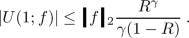

Proof
First split the integral in the definition of U(1; f) as follows:
-
(i)
For the estimate of \(\text {(I)}\), consider the Taylor expansion for f around \(t=0\) keeping in mind that \(f(0)=0\):
$$\begin{aligned} f(t) = tf'(0)+ \frac{t^2}{2} f''\big ({\tilde{t}} \big ) \qquad \text {for suitable }{\tilde{t}}\in [0,t] \,,\end{aligned}$$and therefore
$$\begin{aligned} \text {(I)}&\le \int _{0}^{1/2} \underbrace{\Big | \frac{1}{(1-t)}\Big |}_{\le 2}\Big ( \underbrace{|f'(0)|}_{\le \Vert f\Vert _{C^2}}+\underbrace{|t/2|}_{\le 1/4} \underbrace{|f''({\tilde{t}})|}_{\le \Vert f\Vert _{C^2}}\Big ) \textrm{d}t + \int _{0}^{1/2}\underbrace{\Big | \frac{1}{(1-t)}\Big |}_{\le 2} \underbrace{|f(1)|}_{\le \Vert f\Vert _{C^2}} \textrm{d}t\\&\le \frac{9}{4}\, \Vert f\Vert _{C^2} \end{aligned}$$(note that \({\tilde{t}}\) is actually a function of t, but this is unproblematic because \(f''\) is uniformly bounded).
Similarly, for the estimate of (II) we use the Taylor expansion of f, but now around \(t=1\),
$$\begin{aligned} f(t) = f(1) + (t-1)f'(1)+\frac{(t-1)^2}{2} f''({\tilde{t}}) \qquad \text {for suitable }{\tilde{t}}\in [0,t] \,. \end{aligned}$$We thus obtain
$$\begin{aligned} \text {(II)}&\le \int _{1/2}^{1} \Big | \frac{1}{t(1-t)}\Big |\Big ( |1-t|\,|f(1)|+ |1-t|\,|f'(1)|+\frac{|1-t|^2}{2} |f''({\tilde{t}})|\Big ) \,\textrm{d}t\\&\le \int _{1/2}^{1} \underbrace{|1/t|}_{\le 2}\Big ( \underbrace{|f(1)|}_{\le \Vert f\Vert _{C^2}}+ \underbrace{|f'(1)|}_{\le \Vert f\Vert _{C^2}}+\underbrace{\frac{|1-t|}{2}}_{\le 1/4} \underbrace{|f''({\tilde{t}})|}_{\le \Vert f\Vert _{C^2}}\Big )\, \textrm{d}t \le \frac{9}{4} \Vert f\Vert _{C^2} \,. \end{aligned}$$ -
(ii)
-
(a)
Case \(z=0\): First note that

This yields for \(R< 1/2\),
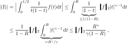
Moreover, the integral (II) vanishes for \(R<1/2\).
-
(b)
Case \(z=1\): Similarly as in the previous case, we now have
$$\begin{aligned} \text {(I)} = 0 \qquad \text {for~R<1/2}\,.\end{aligned}$$Moreover, just as in the previous case, one can estimate

This yields for \(R< 1/2\),
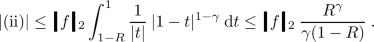
\(\square \)
-
(a)


Now we have all the tools to prove Theorem 5.7.
Proof of Theorem 5.7
Before beginning, we note that the \(u_0\)-limit in (5.8) may be disregarded, because the symbol is translation invariant in position space (see Lemma A.3, noting that \(\mathfrak {a}_{0,1}\) does not depend on \(u\equiv \varvec{x}\) or \(u'\equiv \varvec{y}\)).
The remainder of the proof is based on the idea of the proof of [34, Theorem 4.4] Let \({\mathfrak {a}}\) be the symbol in (5.3). By Lemma 2.10, we can assume that the operator norm of \(\textrm{Op}_\alpha ({\mathfrak {a}})\) is uniformly bounded in \(\alpha \). We want to apply Lemma A.8 with \(\mathcal {A}={\mathfrak {a}}\) and \(\mathcal {B}=I_{\mathcal {J}}\) (recall that \({\mathcal {J}}=(-\infty ,0)\)). In order to verify the conditions of this lemma, we first note that, Remark A.9 (i) yields condition (ii), whereas condition (i) follows from the estimate
(which holds for any \(\psi \in L^2(\mathbb {R})\)). Now Lemma A.8 yields
Since \(P_{\alpha ,{\mathcal {J}}}\) is a projection operator, we see that \(\Vert \textrm{Op}_\alpha (I_{\mathcal {J}} \,{\mathfrak {a}})\Vert _\infty \le \Vert \textrm{Op}_\alpha ({\mathfrak {a}})\Vert _\infty \) for all \(\alpha \). In particular, the operator \(\textrm{Op}_\alpha (I_{\mathcal {J}} \,{\mathfrak {a}})\) is bounded uniformly in \(\alpha \). Hence,
uniformly in \(\alpha \) (recall that \(A({\mathfrak {a}})\) is the symmetric localization from Theorem 5.3). Moreover, the sup-norm of the symbol \(\mathfrak {a}_{0,1}\) itself is bounded by a constant \(C_2\). We conclude that we only need to consider the function g on the interval
Therefore, we may assume that
possibly replacing g by the function
with a smooth cutoff function \(\Psi _C\ge 0\) such that \(\Psi _C|_{[-C+1,C-1]} \equiv 1\) and \({{\,\textrm{supp}\,}}\Psi _C \) \( \subseteq [-C,C]\). For ease of notation, we will write \(g \equiv {\tilde{g}}\) in what follows.
We remark that the function \(\eta _\kappa \) which we plan to consider later already satisfies this property by definition with \(C=2\). From Lemma 2.8 and Lemma 5.8 we see that \(D_\alpha (g,{{\mathcal {K}}},\mathfrak {a}_{0,1})\) is indeed trace class. We now compute this trace, proceeding in two steps.
\(\underline{\hbox {First Step: Proof forg }\in C^2(\mathbb {R}).}\)
To this end, we first apply the Weierstrass approximation theorem as given in [27, Theorem 1.6.2] to obtain a polynomial \(g_\delta \) such that \(f_\delta :=g-g_\delta \) fulfills
Without loss of generality, we can assume that \(f_\delta (0)=0\) (otherwise replace \(f_\delta \) by the function \(t\mapsto f_{\delta /2}(t)- f_{\delta /2}(0)\)). In order to control the error of the polynomial approximation, we apply Lemma 2.6 with \(n=2\), \(r=C\), some \(\sigma \in (0,1)\), \(q=1\) and
(note that here g is the function in Lemma 2.6) where \(\Psi _C\) is the cutoff function from before (the cutoffs and approximation are visualized in Fig. 5).

Visualization of the cutoffs and approximations in the first step of the proof of Theorem 5.7 for \(C=2\). We start with a function g, which is first multiplied by the cutoff-function \(\Psi _C\), giving \({\tilde{g}}\). This function is then approximated by a polynomial \(g_\delta \). Multiplying \(g_\delta \) by the cutoff function \(\Psi _C\) results in a function which is here called \({\tilde{g}}_\delta \) (but does not directly appear in the proof). The function \({\tilde{f}}_\delta \) is then given by the difference between \({\tilde{g}}\) and \({\tilde{g}}_\delta \)
This gives
with an implicit constant independent of \(\delta \) and \(\alpha \). Moreover, applying Lemma 5.8 with \(q=\sigma \), we conclude that for \(\alpha \) large enough
(again with an implicit constant independent of \(\delta \) and \(\alpha \)). Using this inequality, we can estimate the trace by
with a constant \(C_3\) independent of \(\delta \) and \(\alpha \). In order to compute the remaining trace, we can again apply Theorem 5.3 (exactly as in the example (5.6)). This gives
and thus
which yields together with Lemma 5.9,
Moreover, applying Lemma 5.9 to \(f_\delta \) we obtain due the (5.11)
Therefore, taking the limit \(\delta \rightarrow 0\) in (5.12) gives
Analogously, using
we obtain
Now we can take the limit \(\delta \rightarrow 0\),
Combining the inequalities for the \(\limsup \) and \(\liminf \), we conclude that for any \(g\in C^2(\mathbb {R})\),
\(\underline{\hbox {Second Step: Proof for }g\hbox { as in claim.}}\)
By choosing a suitable partition of unity and making use of linearity, it suffices to consider the case \(T=\{z\}\) meaning that g is non-differentiable only at one point z. Next we decompose g into two parts with a cutoff function \(\xi \in C^\infty _0(\mathbb {R})\) with the property that
and writing
with
see also Fig. 6.

Schematic plot of a function g (blue) which is non-differentiable at \(z=0\) with the corresponding functions \(g^{(1)}_{1\!/\!2}\) (red), \(g^{(1)}_{1/4}\) (orange) and \(g^{(1)}_{1/10}\) (green): They are cutting out the non-differentiable point
Note that the derivatives of \(g_R^{(1)}\) satisfy the bounds
(with some numerical constants c(n, k)) and therefore the norm  in Lemma 2.8 can be estimated by

Noting that on the support of \(\big (g_R^{(1)}\big )^{(k)}\) we have
we conclude that

with \(C_4\) independent of R (also note that  is bounded by assumption).
For what follows, it is also useful to keep in mind that
Now we apply (5.13) to the function \(g_R^{(2)}\) (which clearly is in \(C^{2}(\mathbb {R})\)),
Next, we apply Lemma 2.8 to \(g_R^{(1)}\) with A and P as before and some \(\sigma \in (0,1)\) with \(\sigma < \gamma \),

Applying Lemma 5.8 (for \(\alpha \) large enough) with \(q=\sigma \) yields

where the constant \(C_5\) is independent of R and \(\alpha \). Just as before, it follows that

The end result follows just as before by taking the limit \(R\rightarrow 0\), provided that we can show the convergence \(U(1;g_R^{(2)})\rightarrow U(1;g)\) for \(R\rightarrow 0\). To this end note that if \(z\notin \{0,1\}\), we have
for some \(C_6 >0\) independent of R provided that R is sufficiently small (more precisely, so small that \(g_R^{(1)}\) vanishes in neighborhoods around 0 and 1; note that the integrand is supported in \([z-R,z+R]\) and bounded uniformly in R). These estimates show that \(\lim _{R \rightarrow 0} U(1;g-g_R^{(2)}) = 0\) in the case that z is neither 0 nor 1. In the remaining cases where z is either 0 or 1, we can apply Lemma 5.9, which also yields due to (5.14),

This concludes the proof. \(\square \)
We finally apply Theorem 5.7 to the function \(\eta _\kappa \) and the matrix-valued symbol \(\mathcal {A}_0\) (see (1.2) and (4.5)).
Corollary 5.10
For any \(\kappa >0\), \(\eta _{\kappa }\), \({\mathcal {K}}\) and \(\mathcal {A}_0\) as before,
Moreover, in the case that \(\kappa =1\), we can explicitly compute the coefficient \(U(1;\eta _1)\) to give
Proof
As explained in Example 5.6, the functions \(\eta _\kappa \) satisfy Condition 5.5 with \(n=2\) for any \(\kappa >0\). Moreover, we have \(\eta _\kappa (0)=0\) for any \(\kappa >0\). Therefore, we can apply Theorem 5.7 and obtain
Repeating the procedure analogously for \(\mathfrak {a}_{0,2}\) gives
and therefore
By [23, Appendix], evaluating \(U(1;\eta _{\kappa })\) yields
and therefore
This concludes the proof. \(\square \)
Corollary 5.10 already looks quite similar to Theorem 1.1. The remaining task is to show equality in (4.4). To this end, we need to show that all the correction terms drop out in the limits \(u_0 \rightarrow \infty \) and \(\alpha \rightarrow \infty \). The next section is devoted to this task.
6 Estimating the Error Terms
In the previous section, we worked with the simplified kernel (4.5) and computed the corresponding entropy. In this section, we estimate all the errors, thereby proving the equality in (4.4). Our procedure is summarized as follows. Using (3.10), the regularized projection operator \((\Pi _-^\varepsilon )_{kn}\) can be written as
and \(\mathcal {A}^{(\varepsilon )}\) as in (3.12) and the error term
We denote the corresponding symbol by
In preparation, translate \({\mathcal {K}}\) to \({\mathcal {K}}_0\) with the help of the unitary operator \(T_{u_0}\) making use of Lemma A.3. Moreover, we use that the operators \((\Pi _-^\varepsilon )_{kn}\) and \(\textrm{Op}_\alpha (\mathcal {A}_0)\) are self-adjoint. We thus obtain
where \(\mathcal {A}_0\) is the kernel of the limiting operator from (4.5). Note that \(T_{u_0}(\mathcal {A}_0) = \mathcal {A}_0\) since the symbol \(\mathcal {A}_0\) only depends on \(\xi \). Now we can estimate


In the following, we will estimate the expressions (I) and (II) separately.
6.1 Estimate of the Error Term (I)
We begin with the following simplified result from [34], which is related to Lemma 2.8.
Theorem 6.1
[34, Condition 2.3 and Theorem 2.4 (simplified to our needs)] Let f satisfy Condition 2.7 with some \(n\ge 2\) and \(\gamma ,R>0\). Let \(\mathfrak {S}\) be a q-normed ideal of compact operators on \({\mathfrak {H}}\) such that there is \(\sigma \in (0,1]\) with \(\sigma < \gamma \) and
Let \(\mathcal {A},\mathcal {B}\) be two bounded self-adjoint operators on \({\mathfrak {H}}\). Suppose that \(|\mathcal {A}-\mathcal {B}|^\sigma \in \mathfrak {S}\), then

with a positive constant \(C_n\) independent of \(\mathcal {A},\mathcal {B},f\) and R.
In order to apply this theorem to the functions \(\eta _\kappa \), as in the proof of Theorem 5.7 we use a partition of unity. Similar as explained in Example 5.6, we need to choose \(\gamma <1\) for \(\kappa =1\) and \(\gamma \le \min \{1,\kappa \}\) otherwise. We will later see that with the methods in this work we can only estimate the error terms if \(\kappa >2/3\). Thus, we assume that \(2/3<\gamma <1\) allowing us to treat all these cases simultaneously. This gives rise to the constraint
Setting \(\mathcal {A}=\chi _{{\mathcal {K}}_0} \textrm{Op}_\alpha (T_{u_0}(\mathcal {A}_{\textrm{full}}^{(\varepsilon )}))\chi _{{\mathcal {K}}_0}\) and \(\mathcal {B}=\chi _{{\mathcal {K}}_0} \textrm{Op}_\alpha (\mathcal {A}_0)\chi _{{\mathcal {K}}_0}\) (which are clearly bounded and self-adjoint), we obtain
with C independent of \(\mathcal {A}\) and \(\mathcal {B}\) (and thus in particular independent of \(u_0\) and \(\alpha \)).
For ease of notation, from now on we will denote
Note that the symbol of the \(\textrm{Op}_\alpha (.)\) in (6.1) is matrix valued. But, applying Remark 2.4 (ii), we obtain
with scalar-valued symbols \(\Delta ({\mathfrak {a}}_{ij})_{u_0}^{(\varepsilon )}\).
We now proceed by estimating the Schatten norms of the operators
This will also show that these operators are well defined and bounded on \(L^2 \) \(({\mathcal {K}}_0,\mathbb {C})\). For the estimates, we need the detailed form of the symbols given by
with \(r_{ij}(u,u',\xi )=({\mathcal {R}}_0(u,u',\xi ))_{ij}\) for any \(1\le i,j \le 2\). Note that these equations only hold as long as u is smaller than some fixed \(u_2\) which we may always assume as we take the limit \(u_0 \rightarrow - \infty \).
One can group the terms in these functions into three classes, each of which will be estimated with different techniques: There are terms which are supported on “small” intervals \([-m\varepsilon /M,0]\) or \([0,m\varepsilon /M]\). There are terms that contain the factor \(e^{2Mi\xi (u+u_0)/\varepsilon }\), which makes them oscillate faster and faster as \(u \le u_0 \rightarrow -\infty \). And, finally, there are the \(r_{ij}\)-terms which decay rapidly in u and/or \(u'\). Due to the triangle inequality (2.15), it will suffice to estimate each of these classes separately.
6.1.1 Error Terms with Small Support
We use this method for terms which do not depend on u and \(u'\) and which in \(\xi \) are supported in a small neighborhood of the origin. More precisely, these terms are of the form
Since these operators are translation invariant, we do not need to apply the translation operator \(T_{u_0}\). This also shows that the error corresponding to these terms can be estimated independent of \(u_0\). For the estimate, we will apply Proposition 2.14. As an example, consider
and
which are both in \(L^2_{{\textrm{loc}}}(\mathbb {R})\) because \(|f_{0,1}^+|\) is bounded. Moreover, applying Lemma A.5 we obtain:
for
which is again in \(L^2_{{\textrm{loc}}}(\mathbb {R})\) for the same reasons as \(a^{(\varepsilon )}\). Now we apply the Hölder-type inequality (2.16) and Proposition 2.14 with \(p\in (0,1)\) arbitrary to obtain
Next, noting that \({\mathcal {K}}_0 = (-\rho ,0) \subseteq (-\lceil \rho \rceil , 0)\), it follows that
Similarly, since \(|a_{(\varepsilon )}(\omega )|\) is bounded by one,
Combining the last two inequalities, we conclude that
Completely similar for
we obtain
for any \(p\in (0,1)\) so in particular for \(p=\sigma \). The estimates (6.6) and (6.7) show that the error terms with small support are bounded uniformly in \(u_0\) and \(\alpha \). Therefore, dividing by \(\log \alpha \) and taking the limit \(\alpha \rightarrow \infty \), these error terms drop out.
6.1.2 Rapidly Oscillating Error Terms
After translating the symbol by \(u_0\), these error terms are of the form
for some functions \(g, {\tilde{g}}\) which are measurable and bounded. They appear in \(\Delta ({\mathfrak {a}}_{12})_{u_0}^{(\varepsilon )}\) and \(\Delta ({\mathfrak {a}}_{21})_{u_0}^{(\varepsilon )}\). For simplicity, we restrict attention to the symbols of the form \(b^{(\varepsilon )}\), but all estimates work the same for \({\tilde{b}}^{(\varepsilon )}\) in the same way. We will make use of the following results from [5, Theorem 4 on page 273 and p. 254, 263, 273], which adapted and applied to our case of interest can be stated as follows.
Theorem 6.2
Let \(l\in \mathbb {N}_0\) and K be an integral operator on \(L^2({\mathcal {K}}_0)\) (again with \({\mathcal {K}}_0=(-\rho , 0)\)) with kernel k, i.e., for any \(\psi \in L^2({\mathcal {K}}_0)\):
If \(k(.,u') \in W^l_2({\mathcal {K}}_0)\) for almost all \(u' \in {\mathcal {K}}_0\) with
then
and
We want to apply this theorem for \(p\in (0,1)\) arbitrary, thus let \(l\in \mathbb {N}\) arbitrary. Moreover, in view of Lemma A.6, the integral representation corresponding to \(\chi _{{\mathcal {K}}_0} \textrm{Op}_\alpha (b^{(\varepsilon )})\chi _{{\mathcal {K}}_0}\) may be extended to all of \(L^2(\mathbb {R})\) and we may interchange the \(\textrm{d}\xi \) and \(\textrm{d}u'\) integrations. Thus, we need to estimate the norm \(\theta _2\) of the kernel of this operator. Thus, we consider kernels of the form
where we used the change of coordinates \({\tilde{\xi }}= \xi /\varepsilon \). Since g is bounded and the factor \(e^{-\varepsilon M {\tilde{\xi }}}\) provides exponential decay, these kernels are always differentiable up to arbitrary orders with
Our goal is to show that the limit \(u_0 \rightarrow - \infty \) of \(\theta _2\big (k_{u_0}^{(\varepsilon )}\big )\) is uniformly bounded in \(\varepsilon \). To this end, we first note that
with
Now note that both \(h_{1,(\varepsilon )}\) and \(h_{l,(\varepsilon )}\) are in \(L^1(\mathbb {R})\), so the Riemann–Lebesgue Lemma (see, for example, [6, Theorem 1]) tells us that for any \(\delta >0\) we can find \(R=R(\varepsilon )>0\) such that
Keeping in mind that for \(u_0 \le 0\),
this is satisfied for \(u_0 < -R(\varepsilon )\). This yields
which in turn leads to
and so
for any \(p\in (0,1)\), so in particular this holds for \(p=\sigma \). As \(\delta \) is arbitrary, we conclude that the rapidly oscillating error terms vanish in the limit \(u_0 \rightarrow - \infty \). We note for clarity that, since we take the limit \(u_0 \rightarrow -\infty \) first, we do not need to worry about the dependence of the above estimate on \(\varepsilon \).
6.1.3 Rapidly Decaying Error Terms
Finally, we consider the rapidly decaying error terms. In order to determine their detailed form, we first note that the solutions of the radial ODE have the asymptotics as given in Lemma 2.3 with an error term of the form
with
and \(f^\pm \) as in (B.1). Using this asymptotics in the integral representation, the error terms in (6.2)–(6.5) can (similar as explained in AppendixC) computed to be
In order to estimate these terms, the idea is to apply Theorem 6.2 (as well as the \(\sigma \)-triangle inequality) to each of these terms (with u and \(u'\) shifted by \(u_0\)) and then take the limit \(u_0\rightarrow - \infty \). We will do this for the first few terms explicitly, noting that the other terms can be estimated similarly.
Given \(u_2\), we know from Lemma 2.3 that for all \(u<u_2\),
with constants \(c,d>0\) that can be chosen independently of \(\omega \) (note that we always normalize the solutions by \(|f_0|=1\)). Now for any \(a,b \in \{1,2\}\) we consider the symbol
which is contributing to \(r_{11}(u,u',M\xi /\varepsilon )\) (note that we again rescaled here in order to get the correct prefactor \(e^{-i\alpha \xi (u-u')}\)). Translating by \(u_0\) as before gives
By Lemma A.6, the corresponding integral representation can be extended to all of \(L^2(\mathbb {R})\), since \(R_+\) is bounded uniformly in \(\omega \) when restricted to the compact interval \({\mathcal {K}}_0\) due to Lemma 2.3, and the \(e^{M\xi }\)-factor provides exponential decay in \(\omega \). Moreover, Lemma A.6 again implies that we may interchange the \(\textrm{d}\xi \) and \(\textrm{d}u'\) integrations.
In order to estimate the corresponding error term, we apply Theorem 6.2 to the kernel
(note that we could leave out the \(\chi _{{\mathcal {K}}_0}\)-functions because in Theorem 6.2 we consider the operator on \(L^2({\mathcal {K}}_0)\); moreover, we rescaled back as before). This kernel is differentiable for similar reasons as before and
Using again the estimates for \(R_\pm \) in (6.8) yields for any \(u,u ' \in {\mathcal {K}}_0\):
where we used that \(|t_{ab}|, |f_{0,1\!/\!2}^\pm | \le 1\). Therefore,
and thus
which makes clear that the corresponding error term vanishes in the limit \(u_0 \rightarrow - \infty \).
We next consider a u-dependent contribution to \(r_{11}\) for some \(a,b\in \{1,2\}\) whose kernel of the form
Differentiating with respect to u gives
so that, similarly as before,
This gives
and thus
with a constant \(C(\varepsilon )\) independent of \(u_0\). This shows that the corresponding error term again vanishes as \(u_0 \rightarrow \infty \).
All the other error terms contributing to \(r_{ij}\) can be treated in the same way: The absolute value of the corresponding kernels (and their first derivatives) can always be estimated by a factor continuous in u and \(u'\) times a factor exponentially decaying in \(u_0\) like \(e^{\textrm{d}u_0}\). This makes it possible to estimate \(\theta _2\) by a function which decays exponentially as \(u_0 \rightarrow -\infty \).
6.2 Estimate of the Error Term (II)
It remains to estimate the error terms (II) on page 39. First of all note that due to Lemma A.3,
Luckily, in this case we can directly compute \(\eta _\kappa \big ((\Pi _-^\varepsilon )_{kn}\big )\) and \(\eta _\kappa \big (\textrm{Op}_\alpha (\mathcal {A}_0)\big )\), which simplifies the estimate. As explained before in Lemma A.1, we have
Moreover, from Proposition 3.4 and Corollary 3.6 we conclude that for any \(\psi \in C^\infty _0(\mathbb {R}, \mathbb {C}^2)\),
So we conclude that we can rewrite
where the entries of the symbol \({\tilde{\mathcal {A}}}^{(\varepsilon )} = (\Delta \tilde{{\mathfrak {a}}}_{i,j}^{(\varepsilon )})_{1\le i,j\le 2}\) are given by
Thus, these error terms are almost the same as before, except that the factor \(e^{M\xi }\) has been replaced by \(\eta _\kappa (e^{M\xi })\) etc. and without translation by \(u_0\). Therefore, after applying Lemma A.3 in order to again translate by \(u_0\),
we can use the same techniques as before if we can show that the functions
are bounded and in \(L^1(\mathbb {R})\) (and the same for the functions with \(\omega \rightarrow -\omega \), but for simplicity we again omit this case). We start with the case that \(\kappa =1\) and first rewrite these functions in more detail as
The terms \(e^{-\varepsilon \omega } \omega ^k\) with \(k=1,2\) are clearly bounded and in \(L^1(\mathbb {R})\). Moreover,
(where “\(l'H\)” denotes the use of L’Hospital’s rule) showing that these terms are bounded near \(\omega = 0\). Next,
showing that as \(\omega \rightarrow \infty \) those terms decay like \(e^{-\varepsilon \omega }\). Therefore, these terms are also bounded and in \(L^1(\mathbb {R})\). Now let \(\kappa \ne 1\), then
so the functions \(g_1\) and \(g_2\) are bounded. Moreover, \(\eta _\kappa (e^{-\varepsilon \omega })\) decay like \(e^{-{\tilde{\kappa }}\varepsilon \omega }\) with \({\tilde{\kappa }}:=\min \{1,\kappa \}\) for \(\omega \rightarrow \infty \) since
This shows that \(\kappa \ne 1\); the functions \(g_1\) and \(g_2\) are in \(L^1(\mathbb {R})\) as well.
7 Proof of the Main Result
We can now prove our main result.
Proof of Theorem 1.1
Having estimated all the error terms in trace norm and knowing that the limiting operator is trace class (see the proof of Theorem 5.7), we conclude that the operator
is trace class. Moreover, we saw that all the error terms vanish after dividing by \(\log \alpha \) and taking the limits \(u_0\rightarrow - \infty \) and \(\alpha \rightarrow \infty \) (in this order). We thus obtain by Corollary 5.10,
Moreover, since by [23, Appendix],
and recalling that \(\alpha = M / \varepsilon \), we obtain the result. \(\square \)
8 Conclusions and Outlook
To summarize this article, we introduced the fermionic entanglement / Rényi entropy of a Schwarzschild black hole horizon based on the Dirac propagator as

We have shown that we may treat each angular mode separately. This transition enables us to disregard the angular coordinates, which makes the problem essentially one-dimensional in space. Furthermore, in the limiting case we were able to replace the symbol of the corresponding pseudo-differential operator by \(\mathcal {A}_0\) in (4.5) provided that \(\kappa >\frac{2}{3}\). Since this symbol is diagonal matrix-valued, this reduces the problem to one spin dimension. Moreover, because \(\mathcal {A}_0\) is also independent of \(\varepsilon \), the trace with the replaced symbol can be computed explicitly. It turns out to be a numerical constant independent of the considered angular mode.
This leads us to the conclusion that the fermionic entanglement entropy of the horizon is proportional to the number of angular modes occupied at the horizon,

and a similar result holds for the Rényi entropies with \(\kappa >\frac{2}{3}\). This is comparable to the counting of states in string theory [35] and loop quantum gravity [1]. Furthermore, assuming that there is a minimal area of order \(\varepsilon ^2\), the number of occupied modes at the horizon was given by \(M^2/\varepsilon ^2\), which would lead to
Bringing the factor \(\log (M / \varepsilon )\) in (8.1) to the other side, this would mean that, up to lower orders in \(\varepsilon ^{-1}\), we would obtain the enhanced area law

One obvious question is whether this result holds not only in the Schwarzs child geometry, but for more general and physically realistic black holes. The core of our analysis makes use only of the asymptotic form of the Dirac wave functions near the event horizon. This leads to the conjecture that our results should hold for any black hole whose near-horizon geometry coincides with that of Schwarzschild. However, it is not clear to us how to prove this result, because our analysis is based on the integral representation of the Dirac propagator in [8], which holds only in the presence of global spacetime symmetries which allowing for the complete separation of the Dirac equation into a system of ordinary differential equations. We expect that the integral representation could be derived in general static and spherically symmetric black hole spacetimes, but this has not been worked out in the literature. Another generalization which seems possible from the perspective of separation of variables is the extension from Schwarzschild to the Kerr–Newman and 5D Myers–Perry family of rotating black holes, where corresponding integral representations have been derived (see [8, 38]).
Another interesting topic for future research would be to analyze the number of occupied angular momentum modes at the horizon in more detail, in particular for a realistic model where the Schwarzschild black hole arises in the large time asymptotics of a spherically symmetric star undergoing gravitational collapse. Keeping into account the dynamical evolution of the regularization (as described, for example, by the regularized Hadamard expansion [10]), we do not expect that the resulting effective regularization length \(\varepsilon \) will be the same for each angular momentum mode. Therefore, the constant in (1.8) might become n-dependent,
In this case, the counting of occupied states in (1.9) would have to be replaced by a weighted sum,
This weighted sum can be understood as the effective number of occupied states. It might be that the weighted sum remains finite even if an infinite number of angular momentum modes (k, n) are taken into account.
Another interesting extension of our results is to consider more general quasi-free states in particular thermal states. Although our methods still apply in this situation, it is not clear to us which results to expect.
Finally, it seems possible to generalize our results technically as follows. Having mainly the von Neumann entropy function (i.e., \(\kappa =1\)) in mind, we only established estimates for \(R_\pm \) and its first derivative in u. This had the consequence that were not able to estimate the corresponding error terms for Rényi entropies with \(\kappa \le \frac{2}{3}\) with the same methods. However, those methods would also apply for \(\kappa \le \frac{2}{3}\) if one were able to estimate higher derivatives of \(R_\pm \) suitably well. This is another topic for future research.
Notes
Note that such a sequence can always be constructed from an arbitrary sequence \(({\tilde{g}}_n)_{n\in \mathbb {N}}\subseteq C^\infty _0(\mathbb {R})\) converging to g in \(L^1(\mathbb {R})\) by smoothly cutting off the values of the function whenever its absolute value is larger than \(\Vert g\Vert _\infty +1\) (to ensure uniform boundedness) and then going over to a subsequence (to get pointwise convergence a.e., see, for example, [30, Theorem 3.12]).
Note that for any \(A \in \mathfrak {S}_q\) we can write \(\Vert A\Vert _q=(\sum _i \sqrt{\lambda _i}^q)^{1/q}\) where the \(\lambda _i\) are the eigenvalues of \(A^*A\) (note that since A is compact, there are countably many). Moreover, for any eigenvector \(\psi \) of \(A^*A\) corresponding to a non-zero eigenvalue, the vector \(A\psi \) is an eigenvector of \(AA^*\) with the same eigenvalue, so we see that \(\Vert A^*\Vert _q\le \Vert A\Vert _q\) (as \(\psi \) might lie in the kernel of A). Then, symmetry yields the equality.
Since the function \(f(x):=xe^x\) is strictly increasing (and differentiable) on \((0,\infty )\), so is \(W=f^{-1}\) on \(\big (f(0),f(\infty )\big )=(0,\infty )\). So from \(xe^x \ge x\) for any \(x\ge 0\) follows \(x=W(xe^x)\ge W(x)\).
If \(|f(u)|=0\) for one \(u \in \mathbb {R}\), then due to (B.2) any order of derivative of f vanishes at u a and therefore, by the Picard–Lindelöf theorem, the function f vanishes identically on \(\mathbb {R}\).
References
Ashtekar, A., Baez, J.C., Krasnov, K.: Quantum geometry of isolated horizons and black hole entropy,. Adv. Theor. Math. Phys. 4(1), 1–94 (2000)
Bekenstein, J.D.: Statistical black hole thermodynamics. Phys. Rev. D 12, 3077–3085 (1975)
Birman, M.Sh., Karadzhov, G.E., Solomjak, M.Z.: Boundedness conditions and spectrum estimates for the operators \(b(X)a(D)\) and their analogs, Estimates and asymptotics for discrete spectra of integral and differential equations (Leningrad, 1989–90), Adv. Soviet Math., vol. 7, Amer. Math. Soc., Providence, RI, pp. 85–106 (1991)
Birman, M.S., Solomjak, M.Z.: Estimates for the singular numbers of integral operators. Uspehi Mat. Nauk 32(1(193)), 17–84, 271 (1977)
Birman, M.Sh., Solomjak, M.Z.: Spectral theory of selfadjoint operators in Hilbert space, Mathematics and its Applications (Soviet Series), D. Reidel Publishing Co., Dordrecht, 1987, Translated from the 1980 Russian original by S. Khrushchëv and V. Peller
Bochner, S., Chandrasekharan, K.: Fourier Transforms, Annals of Mathematics Studies, No. 19, Princeton University Press, Princeton, N. J.; Oxford University Press, London (1949)
Casini, H., Huerta, M.: Analytic results on the geometric entropy for free fields. J. Stat. Mech. Theory Exp. (2008), no. 1, P01012, 9 arXiv:0707.1300 [hep-th]
Finster, F., Kamran, N., Smoller, J., Yau, S.-T.: The long-time dynamics of Dirac particles in the Kerr-Newman black hole geometry. Adv. Theor. Math. Phys. 7(1), 25–52 (2003)
Finster, F., Kindermann, S., Treude, J.-H.: An Introductory Course on Causal Fermion Systems. In preparation. www.causal-fermion-system.com/intro-public.pdf (2024)
Finster, F., Kraus, M.: The regularized Hadamard expansion. J. Math. Anal. Appl. 491(2), 124340 (2020). arXiv:1708.04447 [math-ph]
Finster, F., Jonsson, R., Lottner, M., Much, A., Murro, S.: Notions of fermionic entropies for causal fermion systems. In preparation
Finster, F., Reintjes, M.: A non-perturbative construction of the fermionic projector on globally hyperbolic manifolds I—Space-times of finite lifetime. Adv. Theor. Math. Phys. 19(4), 761–803 (2015). arXiv:1301.5420 [math-ph]
Finster, F., Röken, C.: Self-adjointness of the Dirac Hamiltonian for a class of non-uniformly elliptic boundary value problems. Ann. Math. Sci. Appl. 1(2), 301–320 (2016). arXiv:1512.00761 [math-ph]
Finster, F., Röken, C.: The fermionic signature operator in the exterior Schwarzschild geometry. Ann. Henri Poincaré 20(10), 3389–3418 (2019). arXiv:1812.02010 [math-ph]
Goldberg, J.N., Macfarlane, A.J., Newman, E.T., Rohrlich, F., Sudarshan, E.C.G.: Spin-\(s\) spherical harmonics and \(\partial \!\!^-\). J. Math. Phys. 8, 2155–2161 (1967)
Hawking, S.W.: Black hole explosions. Nature 248, 30–31 (1974)
Hawking, S.W.: Particle creation by black holes. Commun. Math. Phys. 43(3), 199–220 (1975)
Hawking, S.W.: Black holes and thermodynamics. Phys. Rev. D 13, 191–197 (1976)
Hawking, S.W.: Breakdown of predictability in gravitational collapse. Phys. Rev. D 14, 2460–2473 (1976)
Helling, R., Leschke, H., Spitzer, W.: A special case of a conjecture by Widom with implications to fermionic entanglement entropy, Int. Math. Res. Not. IMRN, no. 7, 1451–1482 arXiv:0906.4946 [math-ph] (2011)
Hollands, S., Sanders, K.: Entanglement Measures and their Properties in Quantum Field Theory, SpringerBriefs in Mathematical Physics, vol. 34, Springer, Cham, 2018 arXiv:1702.04924 [quant-ph]
Klich, I.: Lower entropy bounds and particle number fluctuations in a Fermi sea. J. Phys. A 39(4), L85–L91 (2006)
Leschke, H., Sobolev, A.V., Spitzer, W.: Scaling of Rényi entanglement entropies of the free fermi-gas ground state: a rigorous proof. Phys. Rev. Lett. 112(16), 160403-1-160403–5 (2014). arXiv:1312.6828 [math-ph]
Leschke, H., Sobolev, A.V., Spitzer, W.: Large-scale behaviour of local and entanglement entropy of the free Fermi gas at any temperature. J. Phys. A 49(30), 30LT04, 9 (2016). arXiv:1501.03412 [quant-ph]
Leschke, H., Sobolev, A.V., Spitzer, W.: Trace formulas for Wiener–Hopf operators with applications to entropies of free fermionic equilibrium states. J. Funct. Anal. 273(3), 1049–1094 (2017). arXiv:1605.04429 [math.SP]
Longo, R., Xu, F.: Relative entropy in CFT. Adv. Math. 337, 139–170 (2018). arXiv:1712.07283 [math]
Narasimhan, R.: Analysis on real and complex manifolds, second ed., Advanced Studies in Pure Mathematics, Vol. 1, Masson & Cie, Éditeurs, Paris; North-Holland Publishing Co., Amsterdam-London; American Elsevier Publishing Co., Inc., New York (1973)
Ohya, M., Petz, D.: Quantum entropy and its use, Texts and Monographs in Physics, Springer-Verlag, Berlin (1993)
Rangamani, M., Takayanagi, T.: Holographic Entanglement Entropy, Lecture Notes in Physics, vol. 931, Springer, Cham (2017) arXiv:1609.01287 [hep-th]
Rudin, W.: Real and Complex Analysis, 3rd edn. McGraw-Hill Book Co., New York (1987)
Simon, B.: Trace ideals and their applications, second ed., Mathematical Surveys and Monographs, vol. 120, American Mathematical Society, Providence, RI (2005)
Sobolev, A.V.: Pseudo-differential operators with discontinuous symbols: Widom’s conjecture. Mem. Amer. Math. Soc. 222(1043), vi+104 (2013). arXiv:1004.2576 [math.SP]
Sobolev, A.V.: On the Schatten-von Neumann properties of some pseudo-differential operators. J. Funct. Anal. 266(9), 5886–5911 (2014). arXiv:1310.2083 [math.SP]
Sobolev, A.V.: Functions of self-adjoint operators in ideals of compact operators. J. Lond. Math. Soc. (2) 95(1), 157–176 (2017). arXiv:1504.07261 [math.SP]
Strominger, A., Vafa, C.: Microscopic origin of the Bekenstein–Hawking entropy. Phys. Lett. B 379(1–4), 99–104 (1996). arXiv:hep-th/9601029
Susskind, L.: String theory and the principles of black hole complementarity. Phys. Rev. Lett. 71, 2367–2368 (1993)
’t Hooft, G.: The Holographic principle, hep-th/0003004, Basics and Highlights in Fundamental Physics 72–100 (2001)
Wang, Q.S.: Local Dirac energy decay in the 5D Myers-Perry geometry using an integral spectral representation for the Dirac propagator. Classical Quantum Gravity 39(23), 235016, 16 (2022). arXiv:2207.10658 [gr-qc]
Widom, H.: On a class of integral operators with discontinuous symbol, Toeplitz centennial (Tel Aviv, 1981), Operator Theory: Advances and Applications, vol. 4, Birkhäuser, Basel-Boston, Mass., 1982, pp. 477–500
Acknowledgements
We are grateful to Erik Curiel, José M. Isidro, Claudio F. Paganini, Alexander V. Sobolev and Wolfgang Spitzer for helpful discussions. We would like to thank the referees for valuable feedback. M.L. gratefully acknowledges support by the Studienstiftung des deutschen Volkes and the Marianne-Plehn-Programm.
Funding
Open Access funding enabled and organized by Projekt DEAL.
Author information
Authors and Affiliations
Corresponding author
Additional information
Communicated by Karl-Henning Rehren.
Publisher's Note
Springer Nature remains neutral with regard to jurisdictional claims in published maps and institutional affiliations.
Appendices
A Few Technical Results on Pseudo-Differential Operators
Appendix provides a few technical results on pseudo-differential operators. By \(\textrm{Op}_\alpha (\mathcal {A})\), we always denote an operator as defined in Sect. 2.4.1.
Lemma A.1
Let \(\textrm{Op}_\alpha (\mathcal {A})\) as defined in Sect. 3.3 with \({\mathcal {U}}=\mathbb {R}^d\). If the symbol \(\mathcal {A}\) is hermitian matrix valued, measurable, independent of \(\varvec{x}\) and \(\varvec{y}\), i.e., \(\mathcal {A}(\varvec{x}, \varvec{y},\varvec{\xi })\equiv \mathcal {A}(\varvec{\xi })\) and is uniformly bounded in \(\varvec{\xi }\) (with respect to the ordinary matrix-sup-norm), then \(\textrm{Op}_\alpha (\mathcal {A})\) is well defined and self-adjoint. Moreover, for any Borel function f defined on the spectrum of \(\textrm{Op}_\alpha (\mathcal {A})\), we have
Proof
Note that
where \(\mathcal {A}(./\alpha )\) denotes the matrix-multiplication operator by \(\mathcal {A}(./\alpha )\) and \(\mathcal {F}\) the unitary extension of the Fourier transform on \(L^2(\mathbb {R}^d,C^n)\) (since (A.1) holds for all \(C^\infty _0(\mathbb {R}^d,\mathbb {C}^n)\)-functions and the right-hand side defines a bounded operator on \(L^2(\mathbb {R}^d,\mathbb {C}^n)\)). This also shows that \(\textrm{Op}_\alpha (\mathcal {A})\) is bounded (and therefore well defined) and self-adjoint. Since for any \(\varvec{\xi }\in \mathbb {R}^d\), the matrix \(\mathcal {A}(\varvec{\xi }/\alpha )\) is hermitian matrix valued, the spectral theorem for matrices yields a unitary matrix \(U(\varvec{\xi })\) such that
Using the identification \(L^2(\mathbb {R}^d,\mathbb {C}^n) \cong L^2\big (\{1,\dots , n\}\times \mathbb {R}^d, \mathbb {C}\big )\), the operator U \((\cdot )^{-1}\mathcal {F}^{-1}\) can be interpreted as the unitary transformation form the multiplicative version of the spectral theorem for the operator \(\textrm{Op}_\alpha (\mathcal {A})\) and \({\mathcal {D}}\) as the corresponding function.
Thus, we have
\(\square \)
Remark A.2
A similar argument as in the above proof can be used to prove a criterion on when the integral representation of \(\textrm{Op}_\alpha (\mathcal {A})\) extends to all Schwartz functions. Let \(\mathcal {A}\) be a symbol which only depends on \(\varvec{x}\). Then, just as in the proof of Lemma A.1 we conclude that
Now take an arbitrary Schwartz function \(\phi \in {\mathcal {S}}(\mathbb {R}^d,\mathbb {C}^n)\), then \(\mathcal {F}\phi \) is defined with the usual integral representation. Moreover, since \(\mathcal {F}\) is an automorphism on the Schwartz space \(\mathcal {F}\phi \in {\mathcal {S}}(\mathbb {R}^d,\mathbb {C}^n)\). Furthermore, if the map \(\mathcal {A}(\cdot /\alpha ) \,(\mathcal {F}\phi )(\cdot )\) is in  , the inverse Fourier transform is again given by the usual integral representation meaning that the integral representation of \(\textrm{Op}_\alpha (\mathcal {A})\) extends to \(\phi \).
We conclude that if for any Schwartz function \(\psi \in {\mathcal {S}}(\mathbb {R}^d,\mathbb {C}^n)\), the vector-valued function \(\mathcal {A}(\cdot /\alpha )\, \psi (\cdot ) \in L^1(\mathbb {R}^d,\mathbb {C}^n)\), then the integral representation of \(\textrm{Op}_\alpha (\mathcal {A})\) extends to all Schwartz functions.
This is, for example, the case for any measurable and (in the matrix sup-norm) bounded symbol \(\mathcal {A}\). \(\Diamond \)
The next lemma will be needed for consistency reasons when taking the limit \(u_0 \rightarrow -\infty \):
Lemma A.3
Let \(\textrm{Op}_\alpha (\mathcal {A})\) as in Sect. 3.3, let \(U,V \subset \mathbb {R}^d\) be arbitrary Borel sets and \(\varvec{c}\in \mathbb {R}^d\) an arbitrary vector. For any \(\varvec{x},\varvec{y}, \varvec{\xi }\in \mathbb {R}^d\) we transform a given symbol \(\mathcal {A}\) by
Then there is a unitary transformation \(t_c\) on \(L^2(\mathbb {R}^d, \mathbb {C}^n)\) such that
Moreover, assuming in addition that \(\textrm{Op}_\alpha (\mathcal {A})\) is self-adjoint, we conclude that for any Borel function f,
Proof
We will show that the desired unitary operator is given by the translation operator
(which is obviously unitary). Note that for any Borel set \(W\subseteq \mathbb {R}^d\)
and therefore
By a change of coordinates, we obtain for arbitrary \(\psi \in C^\infty _0(\mathbb {R}^d,\mathbb {C}^n)\)
This shows (A.2).
For (A.3), we make use the multiplication operator version of the spectral theorem. This provides a unitary transformation \(\phi \) and a suitable function g such that
Combined with the previous discussion, this implies
which is the multiplication operator representation of \(\chi _{U+{\varvec{c}}} \,\textrm{op}_\alpha \big (T_{-{\varvec{c}}}(\mathcal {A})\big )\, \chi _{U+{\varvec{c}}}\), because \(\phi \, t_c\) is also a unitary operator. Therefore,
concluding the proof. \(\square \)
Remark A.4
A similar result as Lemma A.3 holds for translations in the \(\varvec{\xi }\)-variable: Let \(\varvec{c}\in \mathbb {R}^d\) be an arbitrary vector. For any \(\varvec{x}, \varvec{y},\varvec{\xi }\in \mathbb {R}^d\) transform a given symbol \(\mathcal {A}\) by
Then, for any \(\psi \in C^\infty _0(\mathbb {R}^d,\mathbb {C}^n)\) and \(\varvec{x}\in \mathbb {R}^d\) we have
This shows that
which implies similar consequences for trace and Schatten norms since the operator \({\mathcal {M}}_{e^{i\alpha \varvec{c}\cdot }}\) is unitary. \(\Diamond \)
Lemma A.5
Let \(\mathcal {A}\) be a symbol such that \(\textrm{Op}_\alpha (\mathcal {A})\) is well defined on \(L^2(\mathbb {R}^d,\mathbb {C}^n)\), let \({\mathcal {K}} \subset \mathbb {R}\) be some measurable subset and \(\alpha ,\beta >0\) some arbitrary constants. Then,
-
(i)
There is a unitary operator \(V_\beta \) on \(L^2(\mathbb {R}^d,\mathbb {C}^n)\) such that
$$\begin{aligned} V_\beta ^{-1} \,\chi _{\mathcal {K}} \,\textrm{Op}_\alpha (\mathcal {A})\, \chi _{\mathcal {K}} \, V_\beta = \chi _{\beta {\mathcal {K}}}\, \textrm{Op}_{ \alpha /\beta }(\mathcal {A}) \,\chi _{\beta {\mathcal {K}}} \,. \end{aligned}$$(A.4)We refer to this as rescaling in position space.
-
(ii)
By rescaling in momentum space, we mean the equality
$$\begin{aligned} \textrm{Op}_\alpha (\mathcal {A}) = \textrm{Op}_{\beta \alpha }\big (\mathcal {A}(\beta \, \cdot )\big )\,. \end{aligned}$$(A.5)
Proof
First, (ii) simply follows by changing coordinates in the \(\varvec{\xi }\)-integral.
For (i) consider the unitary operator \(V_\beta \), which is for any \(\psi \in L^2(\mathbb {R}^d,\mathbb {C}^n)\) defined by
Then, for any \(\psi \in L^2(\mathbb {R}^d,\mathbb {C}^n)\) and \(\varvec{x}\in \mathbb {R}^d\),
and for any \(\psi \in S(\mathbb {R}^d,\mathbb {C}^n)\)
where in the second step we applied a change of coordinates in the \(\varvec{y}\)-integral. \(\square \)
Lemma A.6
Let \(\textrm{Op}_\alpha (\mathcal {A})\) as in Sect. 3.3, such that \(\mathcal {A}\) satisfies
(where \(\Vert .\Vert _{n\times n}\) is the ordinary sup-norm on the \(n\times n\)-matrices). Then the integral representation of \(\textrm{Op}_\alpha (\mathcal {A})\) may be extended to all \(L^2(\mathbb {R}^d,\mathbb {C}^n)\)-functions and the \(\varvec{y}\) and the \(\varvec{\xi }\) integrations may be interchanged. Thus, for any \(\psi \in L^2(\mathbb {R}^d,\mathbb {C}^n)\) and almost any \(\varvec{x}\in \mathbb {R}^d\), the following equations hold
Proof
We first show that, applying the Fubini–Tonelli theorem and Hölder’s inequality, the integrations may be interchanged, by estimating
Next, we want to show that we can extend the integral representation to all \(L^2(\mathbb {R}^d,\mathbb {C}^n)\)-functions, i.e., that the above integral indeed corresponds to \(\big (\textrm{Op}_\alpha (\mathcal {A})\psi \big )(\varvec{x})\). To this end, let \((\psi _n)_{n\in \mathbb {N}}\) be a sequence of \(C^\infty _0(\mathbb {R}^d,\mathbb {C}^n)\)-functions converging to \(\psi \) with respect to the \(L^2(\mathbb {R}^d,\mathbb {C}^n)\)-norm. Then \(\textrm{Op}_\alpha (\mathcal {A})\psi \) is by definition given by
where the convergence is with respect to the \(L^2(\mathbb {R}^d,\mathbb {C}^n)\)-norm. However, going over to a subsequence we can assume that this convergence also holds pointwise outside of a null set \(N\subseteq \mathbb {R}^d\). Moreover, for any \(\varvec{x}\in {{\mathcal {U}}} {\setminus } N\) and we can compute
with \(\Delta \psi _n:= \psi - \psi _n\). Combining this estimate with the pointwise convergence (A.6) in \({{\mathcal {U}}}\setminus N\) yields the claim. \(\square \)
Remark A.7
We want to apply Lemma A.6 to the operator \(\chi _{\mathcal {K}} (\Pi _-^\varepsilon )_{kn} \chi _{\mathcal {K}}\) with \({\mathcal {K}} = (u_0-\rho ,u_0)\). By rescaling as before, we see that this operator is of the form \(\textrm{Op}_\alpha (\mathcal {A}^{(\alpha )})\) with
Note that, apriori, the integral representation of this operator is well defined only for \(C^\infty _0(\mathbb {R})^2\)-functions with support in \({\mathcal {K}}\). In order to extend the integral representation to all \(L^2({\mathcal {K}}, \mathbb {C}^2)\)-functions, it suffices to verify the condition in Lemma A.6. To this end, we note that, due to Lemma 2.3, for given \(u_2>u_0\), we have
for any \(a\in \{1,2\}\), \(i\in \{+,-\}\), \(u<u_2\) and \(\xi \in \mathbb {R}\), where the constants \(c,d>0\) are independent of \(\xi \). Also using that the transmission coefficients \(t_{ab}\) are always bounded by 1/2, we obtain the estimate
for any \(\alpha >0\) with C independent of u, \(u'\) and \(\xi \). Thus, for any \(u \in {\mathcal {K}}\) and \(\alpha >0\) we have
Clearly, the entire expression vanishes for \(u \notin {\mathcal {K}}\).
This shows that we can indeed apply Lemma A.6 to \(\chi _{\mathcal {K}} (\Pi _-^\varepsilon )_{kn} \chi _{\mathcal {K}}\), meaning that the corresponding integral representation can be applied to any \(L^2({\mathcal {K}},\mathbb {C}^2)\)-function, and the \(u'\)- and \(\xi \)-integrations may be interchanged. Moreover, due to the characteristic functions in the symbol, we can even extend the integral representation to all functions in \(L^2(\mathbb {R},\mathbb {C}^2)\). \(\Diamond \)
Lemma A.8
Let \(\mathcal {A}(\varvec{x},\varvec{y},\varvec{\xi })\equiv \mathcal {A}(\varvec{x},\varvec{\xi })\) (i.e., \(\mathcal {A}\) is independent of \(\varvec{y}\)) and \(\mathcal {B}(\varvec{x},\varvec{y},\varvec{\xi })\equiv \mathcal {B}(\varvec{y},\varvec{\xi })\) be symbols such that \(\textrm{Op}_\alpha (\mathcal {A})\) and \(\textrm{Op}_\alpha (\mathcal {B})\) are well defined and the following two conditions hold:
-
(i)
The operator A defined for any \(\psi \in L^2(\mathbb {R}^d, \mathbb {C}^n)\) by
$$\begin{aligned} (A \psi ) (\varvec{x}):= \int _{\mathbb {R}^n} e^{-i\varvec{\xi }\varvec{x}} \,\mathcal {A}(\varvec{x},\varvec{\xi }/\alpha ) \,\psi (\varvec{\xi })\, \textrm{d} \varvec{\xi }\,, \end{aligned}$$is bounded on \(L^2(\mathbb {R}^d, \mathbb {C}^n)\).
-
(ii)
The operator B defined for any \(\psi \in C^\infty _0(\mathbb {R}^d, \mathbb {C}^n)\) by
$$\begin{aligned} (B \psi ) (\varvec{\xi }):= \frac{1}{(2\pi )^d}\int _{\mathbb {R}^n} e^{i \varvec{\xi }\varvec{y}} \, \mathcal {B}(\varvec{y},\varvec{\xi }/\alpha )\, \psi (\varvec{y})\, \textrm{d} \varvec{y}\,, \end{aligned}$$may be continuously extended to \(L^2(\mathbb {R}^d, \mathbb {C}^n)\).
Then
Proof
We first note that, due to condition (i),
as both sides define continuous operators on \(L^2(\mathbb {R}^d, \mathbb {C}^n)\) and agree on the \(C^\infty _0(\mathbb {R}^d, \mathbb {C}^n)\)-functions (where \(\mathcal {F}\) is again the continuous extension of the Fourier transform to the Hilbert space \(L^2(\mathbb {R}^d, \mathbb {C}^n)\)). Similarly, we conclude that
This yields
and for any \(\psi \in C^\infty _0(\mathbb {R}^d, \mathbb {C}^n)\) we have
Note that as \(\textrm{Op}_\alpha (\mathcal {A})\) and \(\textrm{Op}_\alpha (\mathcal {B})\) are bounded operators, so is \(\textrm{Op}_\alpha (\mathcal {A})\, \textrm{Op}_\alpha (\mathcal {B})\). This concludes the proof by continuous extension and by the definition of \(\textrm{Op}_\alpha (\mathcal {A}\mathcal {B})\). \(\square \)
Remark A.9
-
(i)
In what follows, we often apply the previous lemma in the case that
$$\begin{aligned} \mathcal {B}(\varvec{y},\varvec{\xi })= \chi _U(\varvec{\xi }) \end{aligned}$$for some measurable set \(U\subseteq \mathbb {R}^d\). Then condition (ii) of Lemma A.8 is obviously fulfilled, because for any \(\psi \in C^\infty _0(\mathbb {R}^d, \mathbb {C}^n)\) we have
$$\begin{aligned} B \psi = \chi _{\alpha U}\, \mathcal {F}^{-1} \psi \,, \end{aligned}$$and thus
$$\begin{aligned} \Vert B \psi \Vert = \Vert \chi _{\alpha U}\, \mathcal {F}^{-1} \psi \Vert \le \Vert \mathcal {F}^{-1} \psi \Vert = \Vert \psi \Vert \,. \end{aligned}$$ -
(ii)
Moreover, in the following, the symbol \(\mathcal {A}\) is sometimes independent of both \(\varvec{x}\) and \(\varvec{y}\) and bounded by a constant \(C>0\) (with respect to the matrix sup-norm); then, for any \(\psi \in L^2(\mathbb {R}^d, \mathbb {C}^n)\) it follows that
$$\begin{aligned} A \psi = \mathcal {A}(./\alpha )\, \mathcal {F}\psi , \end{aligned}$$and moreover,
$$\begin{aligned} \Vert A \psi \Vert = \Vert \mathcal {A}(./\alpha )\, \mathcal {F}\psi \Vert \le C \Vert \psi \Vert \,. \end{aligned}$$Therefore, condition (i) in Lemma A.8 is also fulfilled.
-
(iii)
Another case we will consider later is that \(\mathcal {A}\equiv a\) is scalar valued, independent of y and continuous with compact support
$$\begin{aligned} {{\,\textrm{supp}\,}}a \subseteq B_l(v) \times B_r(\mu )\,.\end{aligned}$$Then from the following argument we conclude that A also fulfills condition (i) from Lemma A.8. Take \(\psi \in L^2(\mathbb {R}^d)\) arbitrary and consider
$$\begin{aligned}&\int | A\psi (x)|^2\,\textrm{d}x \\&\quad = \int _{B_l(v)} \textrm{d}x \int _{B_r(\mu )} \textrm{d}\xi \int _{B_r(\mu )} \textrm{d}\xi '\, e^{-iu(\xi '-\xi )}\, \overline{\psi (\xi )}\, \psi (\xi ')\,\overline{a(x,\xi /\alpha )}\,a(x,\xi '/\alpha ) \end{aligned}$$Here we may interchange the order of integration due to the Fubini–Tonelli Theorem since
$$\begin{aligned}&\int _{B_l(v)} \textrm{d}x \int _{B_r(\mu )} \textrm{d}\xi \int _{B_r(\mu )} \textrm{d}\xi '\, \Big | \overline{\psi (\xi )}\, \psi (\xi ')\,\overline{a(x,\xi /\alpha )}\,a(x,\xi '/\alpha )\Big | \\&\quad \le C^2\, \text {vol}(B_l(v)) \,\Vert \psi \Vert _{L^1(B_r(\mu ),\mathbb {C}^2)}^2 < \infty \,, \end{aligned}$$where C is a bound for the absolute value of the continuous and compactly supported function a. Note that \(L^2(B_r(\mu ),\mathbb {C}^2) \subseteq L^1(B_r(\mu ),\mathbb {C}^2)\) since \(B_r(\mu )\) is bounded. We then obtain
$$\begin{aligned}&\int | A\psi (u)|^2\,\textrm{d}u\\&\quad = \int \textrm{d}\xi \,\overline{\psi (\xi )} \int \textrm{d}\xi '\, \psi (\xi ') \underbrace{\int \textrm{d}x \,e^{-ix(\xi '-\xi )} \, \overline{a(x,\xi /\alpha )}\,a(x,\xi '/\alpha )}_{=:{\tilde{a}}(\xi ,\xi ')}\\&\quad \le \Vert \psi \Vert \int |\psi (\xi )|\, \Vert {\tilde{a}}(\xi ,.)\Vert \, \textrm{d}\xi \le \Vert \psi \Vert ^2 \sqrt{ \int \textrm{d}\xi \int \textrm{d}\xi ' \,|{\tilde{a}}(\xi ,\xi ')|^2}\,, \end{aligned}$$where the function \({\tilde{a}}\) is again continuous and compactly supported, which makes the last integral finite. We remark that in the last line we again applied Hölder’s inequality twice.
This estimate shows that condition (i) from Lemma A.8 is again satisfied. \(\Diamond \)
Proof of Lemma 2.3
Proof
We follow the proof of [8, Lemma 3.1]. As explained there, employing the ansatz
the vector-valued function f must satisfy the ODE
where \(\lambda \) is an eigenvalue of the operator
(see [8, Appendix 1]) and thus does not depend on \(\omega \) (in contrast with the Kerr–Newman case as explained in [8]). Estimating (B.2) gives
Next, we transform \(r-2M\) to the Regge–Wheeler coordinate,
where W is the inverse log function, i.e., the inverse function of \(x \mapsto xe^x\). An elementary estimateFootnote 3 shows that \(W(x)\le x\) for any \(x\ge 0\), and therefore, we can estimate
where we also used that \(r\ge 2M\). Setting
we can proceed just as in [8, Proof of 3.1]:
Without loss of generality, we can assume that |f| is nowhere vanishingFootnote 4 and divide (B.3) by |f| giving
This yields
From this, we conclude that
which yields
Using this inequality in (B.3), we obtain
which shows that \(\frac{\textrm{d}f}{\textrm{d}u}\) is integrable. Moreover, the function f(u) converges for \(u\rightarrow -\infty \) to
Now integrating (B.5) from \(-\infty \) to \(u<u_2\), we get
Finally, in order to get rid of the factor \(|f(u_2)|\), we make use of (B.4) in the limit \(u\rightarrow -\infty \),
Substituting this in (B.6), we end up with the desired result
with
and
Similarly, removing \(|f(u_2)|\) from (B.5) using (B.7) we obtain
which completes the proof. \(\square \)
Computing the Symbol of \((\Pi _-^\varepsilon )_{kn}\)
In this section, we give a more detailed computation of the symbol of the operator \((\Pi _-^\varepsilon )_{kn}\) for given k and n. Recall that \((\Pi _-^\varepsilon )_{kn}\) is for any function \(\psi \in C_0^\infty (\mathbb {R},\mathbb {C}^2)\) given by
The main task is therefore to determine
To this end, first note that the details of the coefficients \(t_{ab}\) in (2.9) give
Moreover, using the asymptotics of the radial solutions given in Lemma 2.3 the matrix \(X_i(u,\omega )\,X_j(u',\omega )^\dagger \) can for any \(i,j \in \{1,2\}\) be written as
The terms in (C.6)-(C.7) will result in the error matrix \({\mathcal {R}}_0\) and are computed in Sect. 6.1.3. Here we are mainly interested in the terms in (C.5).
Combining our choices of \(f_0\) from Sect. 2.3.4 with (C.5) and (C.2)-(C.4), we obtain
where \(\tilde{{\mathcal {R}}}_0(u,u',\omega )\) consists of the terms (C.6)-(C.7) inserted in the sum (C.1).
In order to rewrite \((\Pi _-^\varepsilon )_{kn}\) as a pseudo-differential operator, we need a prefactor of the form \(e^{-i\omega (u-u')}\) before the symbol. The matrix components in \((*)\) indeed involve such plane waves. However, the (2, 2)-components oscillate with the wrong sign. In order to circumvent this issue, we can use the freedom of coordinate change \(\omega \rightarrow - \omega \) in the \(\textrm{d}\omega \) integration of the (2, 2)- and (1, 2)-components. This yields (3.9).
Regularity of \(\eta _\kappa \)
We now verify in detail that the functions \(\eta _\kappa \) satisfy Condition 5.5.
Lemma D.1
Consider the functions \(\eta _\kappa \) in (1.1). Then for any \(\kappa \ne 1\), \(\eta _\kappa \) satisfies Condition 5.5 with \(T=\{0,1\}\) for any \(\gamma \le \min \{1,\kappa \}\). Moreover, the function \(\eta _\kappa \) in (1.2) satisfies Condition 5.5 with \(T=\{0,1\}\) for any \(\gamma =\kappa \).
Proof
We start with the case that \(\kappa = 1\). Then,
as
(where “\(l'H\)” denotes the use of l’Hospital’s rule) and
Moreover, for any \(t\in (0,1)\) we have
Thus, for any \(\gamma <1\)
and obviously
Therefore, there exists a neighborhood \(U_{0,0}\) of \(z=0\) and a constant \(C_{0,0}\) such that for any \(t \in U_{0,0}\),
Similarly,
yielding a neighborhood \(U_{1,0}\) of \(z=1\) and a constant \(C_{1,0}\) such that for any \(t \in U_{1,0}\):
The other estimates follow analogously by computing the limits
This concludes the proof for the case that \(\kappa =1\).
Next, consider \(\kappa \ne 1\). It is evident that
Moreover, the derivatives of \(\eta _\kappa \) for \(t\in (0,1)\) are given by
Thus, we conclude that for \(\kappa <1\):
so that we may choose \(\gamma \le \kappa \). For \(1<\kappa \le 2\), first note that none of the first derivatives vanishes at \(t=0\) or \(t=1\), so we have
and therefore, we can only take \(\gamma \le 1\). Similarly, for \(\kappa >2\) we have
so we can only take \(\gamma \le 1\) as well. \(\square \)
Rights and permissions
Open Access This article is licensed under a Creative Commons Attribution 4.0 International License, which permits use, sharing, adaptation, distribution and reproduction in any medium or format, as long as you give appropriate credit to the original author(s) and the source, provide a link to the Creative Commons licence, and indicate if changes were made. The images or other third party material in this article are included in the article’s Creative Commons licence, unless indicated otherwise in a credit line to the material. If material is not included in the article’s Creative Commons licence and your intended use is not permitted by statutory regulation or exceeds the permitted use, you will need to obtain permission directly from the copyright holder. To view a copy of this licence, visit http://creativecommons.org/licenses/by/4.0/.
About this article

Cite this article
Finster, F., Lottner, M. The Fermionic Entanglement Entropy of the Vacuum State of a Schwarzschild Black Hole Horizon. Ann. Henri Poincaré (2024). https://doi.org/10.1007/s00023-024-01459-6
Received:
Accepted:
Published:
DOI: https://doi.org/10.1007/s00023-024-01459-6