Existence of Dissipative Solutions to the Compressible Navier-Stokes System with Potential Temperature Transport

Abstract

We introduce dissipative solutions to the compressible Navier-Stokes system with potential temperature transport motivated by the concept of Young measures. We prove their global-in-time existence by means of convergence analysis of a mixed finite element-finite volume method. If a strong solution to the compressible Navier-Stokes system with potential temperature transport exists, we prove the strong convergence of numerical solutions. Our results hold for the full range of adiabatic indices including the physically relevant cases in which the existence of global-in-time weak solutions is open.

1 Introduction

We consider a compressible viscous Newtonian fluid that is confined to a bounded domain $\Omega \subset \mathbb {R}^d$, $d\in \{2,3\}$. Its time evolution is governed by the following system:

$$\begin{aligned} \partial _t\varrho + \mathrm {div}_{\varvec{x}}(\varrho \varvec{u})&= 0 \qquad \qquad \text {in } (0,T)\times \Omega , \end{aligned}$$

(1.1)

(1.2)

$$\begin{aligned} \partial _t(\varrho \theta ) + \mathrm {div}_{\varvec{x}}(\varrho \theta \varvec{u})&= 0 \qquad \qquad \text {in } (0,T)\times \Omega . \end{aligned}$$

(1.3)

Here $\varrho \ge 0$, $\varvec{u}$, p and $\theta \ge 0$ stand for the fluid density, velocity, pressure, and potential temperature, respectively. The viscous stress tensor is given by

(1.4)

where $\mu$ and $\lambda$ are viscosity constants satisfying $\mu > 0$ and $\lambda \ge -\frac{2}{d}\,\mu \,.$ Denoting by $\gamma > 1$ the adiabatic index, the pressure state equation reads

$$\begin{aligned} p(\varrho \theta ) = a(\varrho \theta )^\gamma \,, \qquad a>0\,. \end{aligned}$$

(1.5)

This type of Navier-Stokes equations is often used in meteorological applications; see, e.g., [1] and the references therein. System (1.1)–(1.5) governs the motion of viscous compressible fluids with potential temperature, where diabatic processes and the influence of molecular transport on potential temperature are excluded. Only potential entropy stratification in the initial data is imposed. We refer a reader to Feireisl et al. [2], where the singular limit in the low Mach/Froude number regime of the above Navier-Stokes system with $\gamma > 3/2$ was analyzed. For $\gamma > 9/5$, Bresch et al. [3] showed that the low Mach number limit for the considered system is the compressible isentropic Navier-Stokes equation. In [4] Lukáčová-Medvid’ová et al. use a slightly more complex version of the above system as the basis for their cloud model; see also Chertock et al. [5], where the uncertainty quantification was investigated. Due to the link between potential temperature and entropy, system (1.1)–(1.5) is often reported in the literature as the Navier-Stokes system with entropy transport. To avoid any misunderstanding, we call it in the present paper the Navier-Stokes system with potential temperature transport.

In literature we can find several existence results for the Navier-Stokes system (1.1)–(1.5). The question of stability of weak solutions for $\gamma > 3/2, \, d=3$ was analyzed by Michálek [6]; see also [7], where the stability of weak solutions for the compressible Navier-Stokes equations with a scalar transport was studied for $\gamma > 9/5$ by Lions. Under the assumption $\gamma \ge 9/5$ in the case $d=3$ and $\gamma >1$ in the case $d=2$, system (1.1)–(1.5) is known to admit global-in-time weak solutions; see Maltese et al.  [8, Theorem 1 with $\mathcal {T}(s)=s^\gamma$]. Note that in the aforementioned paper the authors work with the entropy s instead of the potential temperature $\theta$. However, in their framework the specified choice of the function $\mathcal {T}$ yields $s=\theta$. We point out that the physically relevant adiabatic indices $\gamma$ lie in the interval (1, 2] if $d=2$ and in the interval (1, 5/3] if $d=3$. Consequently, in three space dimensions there are physically relevant values of the adiabatic index for which the global-in-time existence of weak solutions remains an open problem for the Navier-Stokes system (1.1)-(1.5).

A simpler model for viscous compressible fluid flow is the barotropic Navier-Stokes system with the state equation $p= a \varrho ^\gamma ,$ $a= \mathrm {const}.$ The first global-in-time existence result for weak solutions of this system allowing general initial data was established in 1998 by Lions [7] for $\gamma \ge 3/2$ if $d=2$ and $\gamma \ge 9/5$ if $d=3$. In 2001, Feireisl, Novotný, and Petzeltová [9] extended Lions’s result to the situation $\gamma >1$ for $d=2$ and $\gamma >3/2$ for $d=3$; see also Feireisl, Karper, Pokorný [10]. To date, the latter is the best available global-in-time existence result for weak solutions for the barotropic Navier-Stokes system. The main obstacle that hampers the derivation of the existence result for $\gamma \le 3/2$ in three space dimensions is the lack of suitable a priori estimates for the convective term $\varrho \varvec{u}\otimes \varvec{u}$. These difficulties are inherited by the full Navier-Stokes-Fourier system that includes an energy equation, too. In [11], Feireisl and Novotný obtained the existence of global-in-time weak solutions for the Navier-Stokes-Fourier system. However, their result holds only for a very restrictive class of state equations. In particular, the natural example of the perfect gas law $p = \varrho \theta$ is still open for the existence of weak solutions. In this context, we refer a reader to [12], where the complete Navier-Stokes-Fourier system for the perfect gas was studied in the context of generalized solutions.

The question of uniqueness of weak solutions remains open in general. However, we have a weak-strong uniqueness principle for the barotropic Navier-Stokes equations. It means that weak and strong solutions to the Navier-Stokes system emanating from the same initial data coincide; see, e.g., Feireisl, Jin, Novotný [13] or Feireisl [14].

In [15], Feireisl et al. introduced a new concept of generalized solutions to the barotropic Navier-Stokes system. They work with the so-called dissipative measure-valued (DMV) solutions that are motivated by the concept of Young measures. In this context, a DMV-strong uniqueness principle was established and the existence of global-in-time DMV solutions for a class of pressure state equations including the barotropic case with $\gamma \ge 1$ was achieved. In our recent work [16], we have extended the DMV-strong uniqueness result to the Navier-Stokes system with potential temperature transport (1.1)–(1.5).

In [17, Chapter 13], Feireisl et al. give a constructive existence proof and demonstrate that DMV solutions to the barotropic Navier-Stokes system can also be obtained by means of a convergent numerical method that was originally developed by Karlsen and Karper [18,19,20,21]. However, their result is based on the assumption that $\gamma >6/5$ if $d=3$ and $\gamma >8/7$ if $d=2$; for the three-dimensional case see also Feireisl and Lukáčová -Medvid’ová [22]. Again, the difficulties

Fig. 1

Strategy for proving convergence of the numerical scheme

for small values of $\gamma$ are related to the convective term in the momentum equation. To overcome this problem we have added the artificial pressure term $h^\eta (\varrho _{h,\Delta t}^k)^2$ to the momentum method of the scheme. This allows us to prove rigorously the existence of a dissipative weak solution to Navier-Stokes system with potential temperature transport for all $\gamma > 1$ by analyzing the convergence of a suitable numerical scheme. To this end, we propose a new version of the mixed finite element-finite volume method of Karlsen and Karper. We note that the artificial pressure approach was used independently in the recent work of Kwon and Novotný [23] also for the Navier-Stokes equations.

The paper is organized as follows: In Sect. 2, we introduce our notion of DMV solutions to the Navier-Stokes system with potential temperature transport and present our main result. Sect. 3 is devoted to the numerical method and the collection of its basic properties. Subsequently, we follow the strategy delineated in Figure 1 to prove the convergence of the numerical scheme: In Sect. 4, we state a discrete energy balance for our method which serves as a basis for several stability estimates. The consistency of the numerical method is established in Sect. 5 and in Sect. 6 we conclude that any Young measure generated by the solutions to our numerical method represents a DMV solution to the Navier-Stokes system with potential temperature transport. In particular, we show that the numerical solutions converge weakly to the expected values with respect to the Young measure and that the convergence of the numerical solutions is strong as long as a strong solution of (1.1)–(1.5) exists. The mesh-related estimates can be found in Appendix A.1.

2 Dissipative Measure-Valued Solutions

Before defining dissipative measure-valued solutions to the Navier-Stokes system with potential temperature transport, we fix the initial and boundary conditions. The Navier-Stokes system with potential temperature transport (1.1)–(1.5) is endowed with the initial data

$$\begin{aligned} \varrho (0,\cdot ) = \varrho _0 \,, \qquad \theta (0,\cdot ) = \theta _{0}\,, \qquad \varvec{u}(0,\cdot ) = \varvec{u}_0\,, \end{aligned}$$

(2.1)

and the no-slip boundary condition

$$\begin{aligned} \varvec{u}|_{[0,T]\times \partial \Omega } = \mathbf {0}\,. \end{aligned}$$

(2.2)

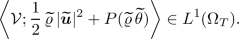
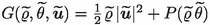
We henceforth write $\Omega _t = (0,t)\times \Omega$ whenever $t>0$. Furthermore, $P:[0,\infty )\rightarrow \mathbb {R}$,

$$\begin{aligned} P(z) = \frac{a}{\gamma -1}\,z^\gamma \,, \end{aligned}$$

(2.3)

is the so-called pressure potential. If $\mathcal {V}=\{\mathcal {V}_{(t,\varvec{x})}\}_{(t,\varvec{x})\,\in \,\Omega _T}$ is a parametrized probability measure (Young measure) acting on $\mathbb {R}^{d+2}$, we write

whenever $g\in C(\mathbb {R}^{d+2})$. Moreover, we tend to write out the function g in terms of the integration variables : if, for example, , then we also write

We proceed by defining dissipative measure-valued solutions to the Navier-Stokes system with potential temperature transport (1.1)–(1.5).

Definition 2.1

(DMV solutions). A parametrized probability measure $\mathcal {V}=\{\mathcal {V}_{(t,\varvec{x})}\}_{(t,\varvec{x})\,\in \,\Omega _T}$ that satisfies¹

and for which there exists a constant $c_\star >0$ such that

is called a dissipative measure-valued (DMV) solution to the Navier-Stokes system with potential temperature transport (1.1)–(1.5) with initial and boundary conditions (2.1) and (2.2) if it satisfies:

• (energy inequality)

  

  and the integral inequality

  

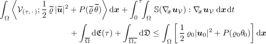  (2.4)

  holds for a.a. $\tau \in (0,T)$ with the energy concentration defect

  

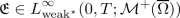
  and the dissipation defect

  $$\begin{aligned} \mathfrak {D}\in \mathcal {M}^+(\,\overline{\Omega _T})\,; \end{aligned}$$

• (continuity equation)

  

  and the integral identity

  

  (2.5)

  holds for all $\tau \in [0,T]$ and all $\varphi \in W^{1,\infty }(\Omega _T)$²;

• (momentum equation)

  

  and the integral identity

  

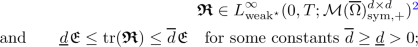
  (2.6)

  holds for all $\tau \in [0,T]$ and all $\varvec{\varphi }\in C^{1}(\,\overline{\Omega _T})^d$ satisfying $\varvec{\varphi }|_{[0,T]\times \partial \Omega }=\varvec{0}$, where the Reynolds concentration defect fulfills³

  

• (potential temperature equation)

  

  and the integral identity

  

  (2.7)

  holds for all $\tau \in [0,T]$ and all $\varphi \in W^{1,\infty }(\Omega _T)$;

• (entropy inequality)

  

  and for any $\psi \in W^{1,\infty }(\Omega _T)$, $\psi \ge 0$, the integral inequality

  

  (2.8)

  is satisfied for a.a. $\tau \in (0,T)$;

• (Poincaré’s inequality)

  there exists a constant $C_P>0$ such that

  

  (2.9)

  for a.a. $\tau \in (0,T)$ and all .

Remark 2.2

Note that the physical entropy S is proportional to $\varrho \ln ( \theta )$. We require that our dissipative solutions satisfy the Second Law of Thermodynamics that is expressed by (2.8) for adiabatic processes. The entropy inequality (2.8) and Poincaré’s inequality (2.9) included in the definition of DMV solutions to the Navier-Stokes system with potential temperature transport are fundamental to guarantee DMV-strong uniqueness; see [16].

We are ready to formulate the main result of this paper: the existence of DMV solutions to the Navier-Stokes system with potential temperature transport.

Theorem 2.3

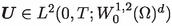
(Existence of DMV solutions). Let $\gamma >1$, $T>0$, $d\in \{2,3\}$, and $\Omega \subset \mathbb {R}^d$ a bounded Lipschitz domain. Further, let and $\varvec{u}_0\in W^{1,2}_0(\Omega )^d$, where

$$\begin{aligned} \varrho _0 > 0 \quad \text {a.e. in } \Omega \qquad \text {and} \qquad c_\star< \theta _{0}< c^\star \quad \text {a.e. in } \Omega \end{aligned}$$

(2.10)

for some constants $0<c_\star < c^\star$. Then there is a DMV solution $\mathcal {V}$ to system (1.1)–(1.5) subject to the initial and boundary conditions (2.1) and (2.2) that additionally satisfies

(2.11)

3 Numerical Scheme

In this section, we present our numerical method, the mixed finite element-finite volume method.

3.1 Spatial discretization

We choose $H\in (0,1)$ and approximate the spatial domain $\Omega \subset \mathbb {R}^d$ by a family $\{\Omega _h\}_{h\,\in \,(0,H]}$ that is related to a family of (finite) meshes $(\mathcal {T}_h)_{h\,\in \,(0,H]}$ by the constraint

$$\begin{aligned} \overline{\Omega _h} = \bigcup _{K\,\in \,\mathcal {T}_h} K \qquad \text {for all } h\in (0,H]. \end{aligned}$$

We assume that the subsequent conditions hold:

• $\Omega _h\subset \Omega$ for all $h\in (0,H]$;

• each element K of a mesh $\mathcal {T}_h$ is a d-simplex that can be written as

  $$\begin{aligned} K = h\mathbb {A}_K (K_{\mathrm {ref}}) + \mathbf {a}_K\,, \qquad \mathbb {A}_K\in \mathbb {R}^{d\times d}\,, \qquad \mathbf {a}_K\in \mathbb {R}^d\,, \end{aligned}$$

  where the reference element $K_{\mathrm {ref}}$ is the convex hull of the zero vector $\varvec{0}\in \mathbb {R}^d$ and the standard unit vectors $\mathbf {e}_{1},\dots ,\mathbf {e}_{d}\in \mathbb {R}^d$, i.e., $K_{\mathrm {ref}} = \mathrm {conv}\{\mathbf {0},\mathbf {e}_{1},\dots ,\mathbf {e}_{d}\}\,$;

• there exist constants $C>c>0$ such that

  $$\begin{aligned} \mathrm {spectrum}(\mathbb {A}_K^T\mathbb {A}_K) \subset [c,C] \qquad \text {for all } K\in {\displaystyle \bigcup _{h\,\in \,(0,H]}}\mathcal {T}_h\,; \end{aligned}$$

• the intersection of two distinct elements $K_1,K_2$ of a mesh $\mathcal {T}_h$ is either empty, a common vertex, a common edge, or (in the case $d=3$) a common face;

• for all compact sets $\mathcal {K}\subset \Omega$ there exists a constant $h_0\in (0,H]$ such that

  $$\begin{aligned} \mathcal {K}\subset \Omega _h \qquad \text {for all } h\in (0,h_0). \end{aligned}$$

  (3.1)

The symbol $\mathcal {E}_{h}$ denotes the set of all faces ($d=3$) or all edges ($d=2$) in the mesh $\mathcal {T}_h$. Further, we define the sets

and, for $K\in \mathcal {T}_h$, the sets

$$\begin{aligned} \mathcal {E}_h(K) = \big \{\sigma \in \mathcal {E}_h\,\big |\,\sigma \subset K\big \} \qquad \text {and} \qquad \mathcal {E}_{h,z}(K) = \big \{\sigma \in \mathcal {E}_{h,z}\,\big |\,\sigma \subset K\big \}\,, \end{aligned}$$

where $z\in \{\mathrm {int},\mathrm {ext}\}$. The elements of $\mathcal {E}_{h,\mathrm {int}}$, $\mathcal {E}_{h,\mathrm {int}}(K)$ and $\mathcal {E}_{h,\mathrm {ext}}$, $\mathcal {E}_{h,\mathrm {ext}}(K)$ are referred to as exterior and interior faces (edges), respectively. In connection with these sets, we introduce the notation

Moreover, we equip each $\sigma \in \mathcal {E}_{h}$ with a unit vector $\varvec{n}_\sigma$ by following the subsequent procedure:

We fix an arbitrary element $K_\sigma \in \mathcal {T}_h$ such that $\sigma \in \mathcal {E}_h(K_\sigma )$ and set $\varvec{n}_\sigma = \varvec{n}_{K_\sigma }(\varvec{x}_\sigma )$. Here, $\varvec{x}_\sigma$ denotes the center of mass of $\sigma$ and $\varvec{n}_{K_\sigma }(\varvec{x}_\sigma )$ is the outward-pointing unit normal vector to the element $K_\sigma$ at $\varvec{x}_\sigma$. Finally, it will be convenient to write $A \lesssim B$ whenever there is an h-independent constant $c>0$ such that $A \le cB$ and $A \approx B$ whenever $A\lesssim B$ and $B\lesssim A$.

3.2 Function Spaces and Projection Operators

We proceed by defining the relevant discrete function spaces. The space of piecewise constant functions is denoted by⁴

For $v\in Q_h$ and $K\in \mathcal {T}_h$ we set $v_K = v(\varvec{x}_K)$, where $\varvec{x}_K$ denotes the center of mass of K. The projection $\Pi _{Q,h}\equiv \overline{\;\cdot \;}:L^2(\Omega )\rightarrow Q_h$ associated with $Q_h$ is characterized by

The Crouzeix-Raviart finite element spaces are denoted by

With these spaces we associate the projection $\Pi _{V,h}:W^{1,2}(\Omega )\rightarrow V_h$ that is determined by

Additionally, we agree on the notation

$$\begin{aligned} Q_h^+ = \big \{v\in Q_h\,\big |\,v|_K > 0 \;\; \text {for all } K\in \mathcal {T}_h\big \}\,, \qquad Q_h^{0,+} = \big \{v\in Q_h\,\big |\,v|_K \ge 0 \;\; \text {for all } K\in \mathcal {T}_h\big \}\,, \\ \varvec{Q}_h = (Q_h)^d\,, \qquad \varvec{V}_h = (V_h)^d\,, \qquad \text {and} \qquad \varvec{V}_{0,h} = (V_{0,h})^d\,. \end{aligned}$$

3.3 Mesh-Related Operators

Next, we define some mesh-related operators. We start by introducing the discrete counterparts of the differential operators and $\mathrm {div}_{\varvec{x}}$. They are determined by the stipulations

respectively. We continue by defining several trace operators. For arbitrary $\sigma \in \mathcal {E}_{h}$, $\varvec{x}\in \sigma$, and

$$\begin{aligned} \varvec{v}\in (Q_h\cup \varvec{Q}_h)\cup (V_h\cup \varvec{V}_h)\cup (C(\overline{\Omega })\cup C(\overline{\Omega })^d) \end{aligned}$$

we put

$$\begin{aligned} \varvec{v}^{\,\mathrm {in},\,\sigma }(\varvec{x}) = \lim _{\delta \,\rightarrow \,0^+}\varvec{v}(\varvec{x}-\delta \varvec{n}_\sigma )\,, \qquad \varvec{v}^{\,\mathrm {out},\,\sigma }(\varvec{x}) =\left\{ \begin{array}{cl} {\displaystyle \lim _{\delta \,\rightarrow \,0^+}\varvec{v}(\varvec{x}+\delta \varvec{n}_\sigma )} &{} \text {if } \sigma \in \mathcal {E}_{h,\mathrm {int}}, \\ \varvec{0} &{} \text {else} \end{array}\right. \,. \end{aligned}$$

Further, we define

The convective terms will be approximated by means of a dissipative upwind operator. For $\sigma \in \mathcal {E}_{h}$, $\varvec{v}\in \varvec{V}_{0,h}$, and $\varvec{r}\in Q_h\cup \varvec{Q}_h$ we put

where $\varepsilon >0$ is a given constant,

$$\begin{aligned} {[}x]^+ = \max \{x,0\}\,, \qquad \text {and} \qquad [x]^- = \min \{x,0\}\,. \end{aligned}$$

Remark 3.1

In the sequel, we tend to omit the letter $\sigma$ in the subscripts and superscripts of the operators defined in Sects 3.2 and 3.3. In some places, we also suppress the letter h and the superscript in in the notation if no confusion arises.

3.4 Time Discretization

In order to approximate the time derivatives, we apply the backward Euler method, i.e., the time derivative is represented by

$$\begin{aligned} D_{t}\varvec{s}^k_h = \frac{\varvec{s}^k_h-\varvec{s}^{k-1}_h}{\Delta t}\,, \end{aligned}$$

where $\Delta t>0$ is a given time step and $\varvec{s}^{k-1}_h$ and $\varvec{s}^k_h$ are the numerical solutions at the time levels $t_{k-1}=(k-1)\Delta t$ and $t_k=k\Delta t$, respectively. For the sake of simplicity, we assume that $\Delta t$ is constant and that there is a number $N_T\in \mathbb {N}$ such that $N_T\Delta t= T$.

3.5 Numerical Scheme

We are now ready to formulate our mixed finite element-finite volume (FE-FV) method.

Definition 3.2

(FE-FV method). A sequence is a solution to our FE-FV method starting from the initial data if the following equations hold for all $k\in \mathbb {N}$, $\phi _h\in Q_h$, and $\varvec{\phi }_h\in \varvec{V}_{0,h}$:

(3.2)

(3.3)

(3.4)

where

$$\begin{aligned} \delta >0 \qquad \text {and} \qquad \nu =\frac{d-2}{d}\mu +\lambda \ge 0\,. \end{aligned}$$

Remark 3.3

We note that our FE-FV method is a generalization of the scheme presented in [17, Chapter 13]. New ingredients are a modified upwind operator and the artificial pressure terms $h^\delta (\varrho _h^k)^2$, . The latter are added to ensure the consistency of our method for values of $\gamma$ close to 1, see Sects 4, 5.

3.5.1 Initial Data

The initial data for the FE-FV method (3.2)–(3.4) are given as

(3.5)

As a consequence of this stipulation, we observe that and

(3.6)

3.5.2 Properties of the Numerical Method

We proceed by summarizing several properties of the FE-FV method (3.2)–(3.4).

Lemma 3.4

Let $k\in \mathbb {N}$ and be given.

• (i) Solvability: There exists a solution to (3.2)–(3.4).

• (ii) Every solution to (3.2)–(3.4) has the following properties:

  • Positivity preservation: . If, in addition, there are constants $0<\underline{c}<\overline{c}$ such that in $\Omega _h$, then in $\Omega _h$.

  • Conservation:

Proof

For the proof we refer the reader to Appendix A.3. $\square$

From Lemma 3.4 we easily deduce the following corollary.

Corollary 3.5

Any solution to the FE-FV method (3.2)–(3.4) starting from the discrete initial data (3.5) has the following properties:

• (i) For every $k\in \mathbb {N}$, $\varrho _h^k>0$ in $\Omega _h$ and in $\Omega _h$.

• (ii) It fulfills and for all $k\in \mathbb {N}$.

4 Stability

We continue by discussing the stability of the FE-FV method (3.2)–(3.4) that follows from a discrete energy balance. For its derivation, we rely on the concept of (discrete) renormalization. The same technique will be used to establish a discrete entropy inequality.

4.1 Discrete Renormalization

In the sequel, we shall state renormalized versions of (3.2) and (3.3) that describe the evolution of $b(\varrho _h^k)$ and $b(\varrho _h^k\theta _{h}^{k})$, $\varrho _h^k b(\theta _{h}^{k})$, respectively, where . Together with suitable choices for the function b, the first two renormalized equations will help us to handle the pressure terms when deriving the discrete energy balance. The last equation will be used to establish the discrete entropy inequality.

Lemma 4.1

Let $(\varrho _h^k,\theta _{h}^{k},\varvec{u}_h^k)_{k\,\in \,\mathbb {N}}$ be a solution to the FE-FV method (3.2)–(3.4) starting from the discrete initial data (3.5). Further, let $(r_h^k)_{k\,\in \,\mathbb {N}_0}\in \{(\varrho _h^k)_{k\,\in \, \mathbb {N}_0},(\varrho _h^k\theta _{h}^{k})_{k\,\in \,\mathbb {N}_0}\}$. Then for every

• (i) there exist values $(\xi ^{(1)}_{r,b,k,\sigma })_{\sigma \, \in \,\mathcal {E}_{\mathrm {int}}},(\xi ^{(2)}_{r,b,k,\sigma })_{\sigma \,\in \,\mathcal {E}_{\mathrm {int}}}\subset \mathbb {R}$ satisfying

  

  and a function $\xi _{r,b,k}\in Q_h$ satisfying

  $$\begin{aligned} \min \{r^{k-1}_h,r^k_h\}\le \xi _{r,b,k}\le \max \{r^{k-1}_h,r^k_h\} \end{aligned}$$

  such that

  

  (4.1)

• (ii) there exist values $(\zeta ^{(1)}_{b,k,\sigma })_{\sigma \,\in \,\mathcal {E}_{\mathrm {int}}},(\zeta ^{(2)}_{b,k,\sigma })_{\sigma \,\in \,\mathcal {E}_{\mathrm {int}}}\subset \mathbb {R}$ satisfying

  $$\begin{aligned} \min \{(\theta _{h}^{k})^{\mathrm {in},\sigma } (\varvec{x}_\sigma ),(\theta _{h}^{k})^{\mathrm {out},\sigma } (\varvec{x}_\sigma )\}\le \zeta ^{(1)}_{b,k,\sigma },\zeta ^{(2)}_{b,k,\sigma } \le \max \{(\theta _{h}^{k})^{\mathrm {in},\sigma }(\varvec{x}_\sigma ), (\theta _{h}^{k})^{\mathrm {out},\sigma }(\varvec{x}_\sigma )\} \end{aligned}$$

  and a function $\zeta _{b,k}\in Q_h$ satisfying

  

  such that

  

  (4.2)

  for all $\psi _h\in Q_h$.

Proof

The proof of assertion (i) can be found in [19, Lemma 5.1]. The main idea is to take $\phi _h=b^{\prime }(\varrho ^k_h)\mathbbm {1}_{\overline{\Omega _h}}$ in (3.2) and $\phi _h=b^{\prime }(\varrho ^k_h\theta _{h}^{k})\mathbbm {1}_{\overline{\Omega _h}}$ in (3.3) and to rewrite the results by means of basic algebraic manipulations, Gauss’s theorem, and Taylor expansions.

Assertion (ii) can be proven similarly; see, e.g., [24, Lemma A.1 with $h^{1-\varepsilon }$ replaced by $h^\varepsilon /2$]. Here, one chooses $\phi _h=b^{\prime }(\theta _{h}^{k})\psi _h$ in (3.3). $\square$

4.2 Discrete Energy Balance

We now have all necessary tools at hand to establish the energy balance for our numerical method.

Lemma 4.2

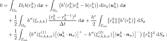
Let $(\varrho _h^k,\theta _{h}^{k},\varvec{u}_h^k)_{k\,\in \,\mathbb {N}}$ be a solution to the FE-FV method (3.2)–(3.4) starting from the discrete initial data (3.5) and P the pressure potential introduced in (2.3). Denoting the discrete energy at the time level $k\in \mathbb {N}_0$ by

$$\begin{aligned} E_h^k\equiv E_h^k(\varrho _h^k,\theta _{h}^{k},\varvec{u}_h^k) = \int _{\Omega _h}\left[ \,\frac{1}{2}\,\varrho _h^k|\overline{\varvec{u}_h^k}|^2 +P(\varrho _h^k\theta _{h}^{k})+h^\delta \big ((\varrho _h^k)^2+(\varrho _h^k \theta _{h}^{k})^2\big )\right] \mathrm {d}\varvec{x}\,, \end{aligned}$$

(4.3)

we deduce that

(4.4)

for all $k\in \mathbb {N}$, where $\xi _{\varrho \theta ,P,k}\in Q_h$ and $(\xi ^{(1)}_{\varrho \theta ,P,k,\sigma })_{\sigma \,\in \,\mathcal {E}_{\mathrm {int}}}, (\xi ^{(2)}_{\varrho \theta ,P,k,\sigma })_{\sigma \,\in \,\mathcal {E}_{\mathrm {int}}}\subset \mathbb {R}$ are chosen as in Lemma 4.1(i).

Proof

The proof can be done following the arguments in [10, Chapter 7.5]. Therefore, we depict only the most important steps. First, taking $\varvec{\phi }_h=\varvec{u}_h^k$ in (3.4) yields

(4.5)

Next, we observe that

(4.6)

Then, we use $\phi _h=\frac{1}{2}|\overline{\varvec{u}_h^k}|^2$ as a test function in (3.2) to deduce that

(4.7)

Moreover, by applying Lemma 4.1(i) with $b=P$ and $b=h^\delta (\cdot )^2$, we obtain

(4.8)

(4.9)

(4.10)

Plugging (4.6)–(4.10) into (4.5), we see that we have almost arrived at (4.4). Indeed, it only remains to show that

which follows by direct calculations. This completes the proof. $\square$

4.3 Time-Dependent Numerical Solutions and Energy Estimates

Next, we formulate appropriate stability estimates for the time-dependent numerical solutions introduced below.

Definition 4.3

Let $(\varrho _h^k,\theta _{h}^{k},\varvec{u}_h^k)_{k\,\in \,\mathbb {N}}$ be a solution to the FE-FV method (3.2)–(3.4) starting from the initial data . We define the functions

$$\begin{aligned} \varrho _h,\theta _{h}:\mathbb {R}\times \Omega \rightarrow \mathbb {R}\,, \quad \varvec{u}_h:\mathbb {R}\times \Omega \rightarrow \mathbb {R}^d\,, \end{aligned}$$

that are piecewise constant in time by setting

The most important stability estimates that can be obtained from the discrete energy balance (4.4) read as follows.

Corollary 4.4

(Stability estimates). Any solution $(\varrho _h,\theta _{h},\varvec{u}_h)$ to the FE-FV method (3.2)–(3.4) starting from the initial data (3.5) has the following properties:

(4.11)

(4.12)

(4.13)

(4.14)

(4.15)

(4.16)

(4.17)

(4.18)

(4.19)

(4.20)

where $q\in [1,\infty )$ if $d=2$ and $q\in [1,6]$ if $d=3$.

Proof

The proof is provided in Appendix A.4. $\square$

4.4 Discrete Entropy Inequality

We conclude this section by stating a discrete entropy inequality. It is obtained by taking $b=\chi$ in Lemma 4.1(ii).

Lemma 4.5

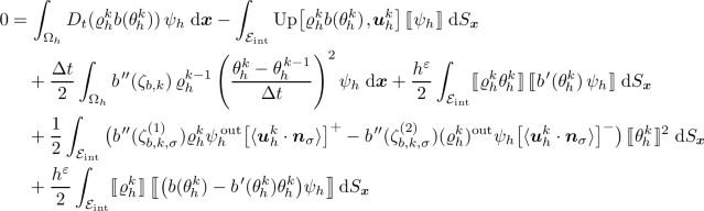
Let $(\varrho _h^k,\theta _{h}^{k},\varvec{u}_h^k)_{k\,\in \,\mathbb {N}}$ be a solution to the FE-FV method (3.2)–(3.4) starting from the discrete initial data (3.5) and a concave function. Then

(4.21)

for all $\psi _h\in Q_h^{0,+}$.

5 Consistency

The goal of this section is to establish the consistency of the FE-FV method (3.2)–(3.4).

Theorem 5.1

(Consistency of the FE-FV method). Let $d\in \{2,3\}$. Further, suppose $(\varrho _h,\theta _{h},\varvec{u}_h)_{h\,\in \,(0,H]}$ is a family of solutions to the FE-FV method (3.2)–(3.4) with

$$\begin{aligned} \gamma> 1\,, \qquad \Delta t\approx h\,, \qquad \varepsilon > 1, \qquad \text {and} \qquad 0<\delta <\tfrac{1}{2} \end{aligned}$$

(5.1)

starting from the initial data defined in (3.5). Then, for $\beta =\min \left\{ \varepsilon -1,\tfrac{1-2\delta }{4}\right\}$,

(5.2)

for all as ,

(5.3)

for all as ,

(5.4)

for all as , and

(5.5)

for all , $\psi \ge 0$, as .

The structure of the proof of Theorem 5.1 is essentially the same as that of [17, Theorem 13.2]. In particular, we will use similar tools. Apart from the estimates listed in Appendix A.1, we will need the following results.

Lemma 5.2

Let , $(r_h^k)_{k\,\in \,\mathbb {N}_0}\subset Q_h$, and define $r_h:\mathbb {R}\times \Omega \rightarrow \mathbb {R}$ via

Then the subsequent relations hold:

(5.6)

(5.7)

Lemma 5.3

Let $r,f\in Q_h$, $\varvec{v}\in \varvec{V}_{0,h}$, and . Then⁵

(5.8)

Corollary 5.4

Let $\varvec{s},\varvec{g}\in \varvec{Q}_h$, $\varvec{w}\in \varvec{V}_{0,h}$, and . Then

(5.9)

Remark 5.5

The formula in Lemma 5.3 also holds true when the dissipative upwind term is replaced by the usual upwind term and the last term on the right-hand side of the identity is canceled. The same applies to Corollary 5.4.

Lemma 5.6

Let $r\in Q_h$, $v\in V_{0,h}$, , and . Then

(5.10)

(5.11)

For the proof of the Lemmata 5.2, 5.3, and 5.6, we refer to [17, Preliminaries, Lemma 8], [10, Chapter 9.2, Lemma 7 with $\chi =1$], and [10, Chapter 9.3, Lemma 8], respectively. For the proof of Lemma 5.3, we additionally need to observe that

which follows from the fact that $r\in Q_h$. Corollary 5.4 can be proven by applying Lemma 5.3 with $(r,f,\varvec{v},\phi )=(s_i,g_i,\varvec{w},\psi _i)$, $i\in \{1,\dots ,d\}$.

Having all necessary tools at our disposal, we can approach the proof of Theorem 5.1.

Proof of Theorem 5.1

Let , $\psi \ge 0$, and be arbitrary test functions. We set $\varphi _h=\Pi _{Q}\varphi$, $\psi _h=\Pi _{Q}\psi$, $\varvec{\varphi }_h = \Pi _{V}\varvec{\varphi }$ and make the following introductory observations:

• Due to the construction of the family $(\Omega _h)_{h\,\in \,(0,H]}$, we have , provided $h\in (0,H]$ is sufficiently small (cf. (3.1)), which we henceforth assume.

• Recall that the elements of $Q_h$ and $V_h$ vanish outside $\Omega _h$. This allows us to replace $\Omega _h$ by $\Omega$ when appropriate.

The continuity equation.

From (3.2) we deduce that

(5.12)

Applying the first estimate in Lemma 5.2 with $(r_h,\phi )=(\varrho _h,\varphi )$ as well as (A.15), the second estimate in (4.11), and the fact that $\Delta t\approx h$, we obtain

where

Next, let us consider the second term on the left-hand side of (5.12). Using Lemma 5.3 with $(r,\varvec{v},f,\phi )=(\varrho _h,\varvec{u}_h,\varphi _h,\varphi )(t,\cdot )$, $t\in [0,T]$, as well as the estimates (A.4)–(A.6) and (A.11), we deduce that

where

These terms can be further estimated as follows.

• Term $|I_{2,h}|$. Due to (4.19), we obtain

  

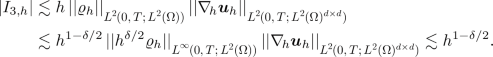
• Term $|I_{3,h}|$. By means of Hölder’s inequality, the second estimate in (A.2), the first estimate in (A.1), the second estimate in (4.13), and the first estimate in (4.12), we derive

  

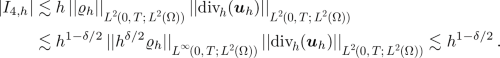
• Term $|I_{4,h}|$. Employing Hölder’s inequality, the second estimate in (4.12), and the second estimate in (4.13), we conclude that

  

• Term $|I_{5,h}|$.

  Applying the first estimate in (A.1) and the second estimate in (4.11), we get

  

Consequently,

(5.13)

with $\alpha _1 = \min \left\{ \varepsilon ,\frac{1-\delta }{2}\right\} >0$ as . Next, using Hölder’s inequality, the first estimate in (A.2), the second estimate in (4.13), and the first estimate in (4.12), we see that

(5.14)

Therefore, we may rewrite (5.13) as

The potential temperature equation.

The proof of (5.3) can be done by repeating the proof of (5.2) with $\varrho _h$ and $\varrho _h^0$ replaced by $\varrho _h\theta _{h}$ and , respectively.

The momentum equation.

From (3.4) we deduce that

(5.15)

Let us consider the first term on the left-hand side of (5.15). Due to the second estimate in Lemma 5.2 with $(r_h,\phi )=(\varrho _h \overline{u_{h,i}},\varphi _i)$, $i\in \{1,\dots ,d\}$, as well as Remark A.1, Hölder’s inequality, the third estimate in (4.11), and the fact that $\Delta t\approx h$, we have

where

Next, we turn to the last three terms on the left-hand side of (5.15). It follows from Lemma 5.6 that

Finally, let us examine the second term on the left-hand side of (5.15). Applying Corollary 5.4 with $(\varvec{s},\varvec{w},\varvec{g},\varvec{\psi })=(\varrho _h\overline{\varvec{u}_h}, \varvec{u}_h,\varvec{\varphi }_h,\varvec{\varphi })(t,\cdot )$, $t\in [0,T]$, as well as the estimates (A.7)–(A.9) and (A.12), we deduce that

where

We continue by estimating the above terms.

• Term $|J_{2,h}|$. We observe that , which implies

  

  (5.16)

  Employing Hölder’s inequality, (4.18), (A.3), the first estimate in (A.1), the first and third estimate in (4.12), and the second estimate in (4.13), we see that

  

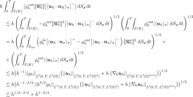  (5.17)

  Next, using Hölder’s inequality, the estimates (A.1), (A.3), (4.15), the first and third estimate in (4.12), the second estimate in (4.13), and the fact that $\Delta t\approx h$, we deduce that

  

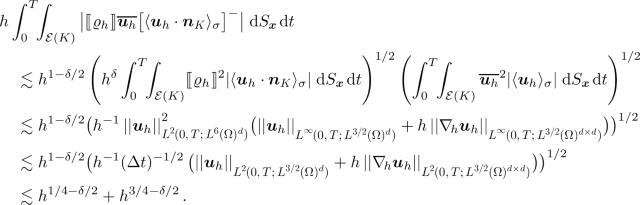  (5.18)

  Consequently, plugging (5.17) and (5.18) into (5.16), we obtain

  $$\begin{aligned} |J_{2,h}| \lesssim h^{1/2-\delta /4} + h^{1-\delta /4} + h^{1/4-\delta /2} + h^{3/4-\delta /2}\,. \end{aligned}$$

• Term $|J_{3,h}|$. Applying Hölder’s inequality, the first estimate in (A.1), the second estimate in (A.2), the first estimate in (4.12), and the second estimate in (4.14), we conclude that

  

• Term $|J_{4,h}|$. Employing Hölder’s inequality, the first estimate in (4.12), and the second estimate in (4.14), we obtain

  

• Term $|J_{5,h}|$.

  Using the first estimate in (A.1) and the third estimate in (4.11), we deduce that

  

Consequently, we have

(5.19)

with $\alpha _2 = \min \left\{ \varepsilon ,\frac{1-2\delta }{4}\right\} >0$ as . Then, using Hölder’s inequality, the first estimate in (A.2), the second estimate in (4.14), and the first estimate in (4.12), we deduce that

Hence, we may rewrite (5.19) as

as .

The entropy inequality.

Taking $\chi =\ln$ in Lemma 4.5, we deduce that

(5.20)

where

Now we may rewrite the first two integrals in (5.20) following the procedure used to handle the continuity equation. We arrive at

(5.21)

where for $j\in \{1,\ldots ,4\}$ the error term $H_{j,h}$ equals $I_{j,h}$ with $\varrho _h$ replaced by $\varrho _h\ln (\theta _{h})$ and $\varphi _h$ replaced by $\psi _h$. Here, it is to be noted that the analogue of the error term $I_{5,h}$ will not be there since (5.20) contains the usual upwind operator $\mathrm {Up}\left[ \,\cdot \,,\,\cdot \,\right]$ instead of the dissipative upwind operator $F_h^{\,\mathrm {up}}\left[ \,\cdot \,,\,\cdot \,\right]$. Since $H_{5,h}=-I_{5,h}$, $c_\star \le \theta _{h}\le c^\star$ and

for every $(k,\sigma )\in \mathbb {N}\times \mathcal {E}_{\mathrm {int}}$ and suitably chosen values $(\eta _{\theta ,k,\sigma })_{\sigma \,\in \,\mathcal {E}_{\mathrm {int}}}\subset [c_\star ,c^\star ]$, it is easy to see that

$$\begin{aligned} |H_{j,h}| \lesssim h^{\alpha _1} \qquad \text {for } 1\le j\le 5. \end{aligned}$$

Moreover, combining $c_\star \le \theta _{h}\le c^\star$ with Hölder’s inequality, the first estimate in (A.1), the second estimate in (4.11) and the first estimate in (4.13), we deduce that

$$\begin{aligned} |H_{6,h}|\,,|H_{7,h}| \lesssim h^{\varepsilon -1}\,. \end{aligned}$$

Finally, seeing that (by a computation similar to that in (5.14)) we have

we may rewrite (5.21) as

where $\alpha _3=\min \{\alpha _1,\varepsilon -1\}$. In particular, we can choose $\beta =\min \{\alpha _1,\alpha _2,\alpha _3\}=\min \left\{ \varepsilon -1, \tfrac{1-2\delta }{4}\right\}$. $\square$

6 Convergence

We proceed by proving our main result, namely Theorem 2.3.

Proof of Theorem 2.3

Let be a sequence of solutions to the FE-FV method (3.2)–(3.4) starting from the initial data defined in (3.5). Here we suppose that the parameters satisfy (5.1).

Due to the second estimate in (4.11), the first estimate in (4.13), the third estimate in (4.12), (A.15), and Corollary 3.5(i), the sequence generates a Young measure that satisfies

Taking into account the remaining estimates in (4.11)–(4.14) as well as the first estimate in (A.2) and passing to a subsequence as the case may be, we obtain that

(6.1)

(6.2)

(6.3)

(6.4)

(6.5)

(6.6)

(6.7)

as Here we have added a w to the standard bar notation for the weak limits to avoid any confusion with the projection operator $\overline{\,\cdot \,}\equiv \Pi _{Q,h}$. Following the arguments given in [10, Chapter 10.2.1, pp. 139 and 142/143], we deduce that

(6.8)

Moreover, using Hölder’s inequality, (A.15), the first estimate in (A.2), the assumption on the initial data, and Lemma A.2, we easily verify that

(6.9)

(6.10)

(6.11)

as .

Energy inequality.

From the discrete energy balance (4.4) we derive that

for all , $\phi \ge 0$. Due to (6.11), (6.4), (6.6), and (6.7), we may perform the limit to obtain

(6.12)

for all , $\phi \ge 0$. Furthermore, we make the subsequent observations:

• In view of the first estimate in (4.11) and the first in (4.13), we may apply [17, Chapter 5, Proposition 5.2] to see that

  

  (6.13)

  Moreover, we may use [15, Lemma 2.1] with $F\equiv 0$ and to deduce that

  

• Applying measure-theoretic arguments to the viscous terms, we conclude that

  

• Using the density of in $W^{1,2}_0(\Omega )$ as well as Gauss’s theorem, we easily verify that

  

In particular, we may rewrite (6.12) in the form

Continuity equation.

In view of (6.1), (6.2), and (6.9), we may perform the limit in (5.2). We obtain

(6.14)

for all . Following the arguments presented in [17, Chapter 2.1.3], we deduce from (6.14) that . Consequently, (6.14) can be rewritten in the form

(6.15)

for all $\tau \in [0,T]$ and . Here, we have set $\mathcal {V}_{(0,\varvec{x})} = \delta _{(\varrho _0(\varvec{x}),\theta _{0}(\varvec{x}),\varvec{u}_0(\varvec{x}))}^{[6]}.$⁶ Due to the integrability properties of and , the boundedness of $\Omega _T$, the fact that is dense in $W^{1,p}(\Omega _T)$ for every $p\in [1,\infty )$, and the Sobolev embedding $W^{1,q}(\Omega _T)\hookrightarrow C(\overline{\Omega _T})$ for $q>d+1$, we may extend the validity of (6.15) to test functions $\varphi$ of the class $W^{1,\infty }(\Omega _T)$.

Potential temperature equation.

The potential temperature equation can be handled in the same manner as the continuity equation.

Momentum equation.

Thanks to (6.3)–(6.5), (6.8), and (6.10), we can take the limit in (5.4). We obtain

(6.16)

for all . Next, we make the following observations:

• Analogous to above, it follows from (6.16) that .

• Using Gauss’s theorem, we conclude that

  

• Due to (6.13), . Moreover, applying [15, Lemma 2.1] with $F\equiv 0$ and , $\xi \in \mathbb {R}^d$, we deduce that

  

  In particular,

  $$\begin{aligned} \underline{d}\mathfrak {E} \le \mathrm {tr}[\varvec{\mathfrak {R}}] \le \overline{d}\mathfrak {E}\,, \quad \text {where} \quad \underline{d} = \min \{2,d(\gamma -1)\} \quad \text {and} \quad \overline{d} = \max \{d,d(\gamma -1)\}\,. \end{aligned}$$

Consequently, (6.16) can be rewritten as

(6.17)

for all $\tau \in [0,T]$ and all . It is easy to see that (6.17) also holds for test functions $\varvec{\varphi }$ of the class . Moreover, for every satisfying $\varvec{\varphi }|_{[0,T]\times \partial \Omega }=\varvec{0}$ we can construct a sequence of smoothed truncations of $\varvec{\varphi }$ such that

Accordingly, we may use the dominated convergence theorem to extend the validity of (6.17) to test functions satisfying $\varvec{\varphi }|_{[0,T]\times \partial \Omega }=\varvec{0}$.

Poincaré’s inequality.

Let $\tau \in [0,T]$ and be arbitrary. Further, let $\{\vartheta _k\}_{k\,\in \,\mathbb {N}}\subset C_c(\mathbb {R}^{d+2})$ be the sequence of functions defined by

and $C\ge 1$ a constant such that

(6.18)

(6.19)

Clearly, such a constant exists due to (A.10) and the usual Poincaré inequality. Due to (6.19), we observe that

Using the monotone convergence theorem, Lemma A.3, Lemma A.2(ii), (iii), the first estimate in (A.2), the first estimate in (4.12), and (6.3), we deduce that

(6.20)

for almost all $\tau \in (0,T)$. Consequently, choosing $C_P=48C^{\,2}/\mu$ we obtain

Entropy inequality.

Due to (6.1), (6.2), and (6.9), we may take the limit in (5.5). We obtain

(6.21)

for all , $\psi \ge 0$. By an approximation argument similar to that in the case of the continuity equation, the validity of (6.21) can be extended to test functions $\psi \ge 0$ of the class $C_c([0,T)\times \overline{\Omega })\cap W^{1,\infty }(\Omega _T)$. In particular, we may consider test functions of the form $\psi =\phi _{\tau ,\overline{\delta }}\,\eta$, where $\eta \in W^{1,\infty }(\Omega _T)$, $\eta \ge 0$, $\tau \in (0,T)$, , and $\phi _{\tau ,\overline{\delta }}\in C_c([0,T))$,

Consequently,

for all $\eta \in W^{1,\infty }(\Omega _T)$, $\eta \ge 0$, $\tau \in (0,T)$, . The entropy inequality (2.8) follows by performing the limit in the above inequality. For the limit process, we rely on Lebesgue’s differentiation theorem as well as the dominated convergence theorem. This completes the proof of Theorem 2.3.

$\square$

From the proof of Theorem 2.3 it follows that any Young measure generated by a sequence obtained from a sequence of solutions to our FE-FV method (3.2)–(3.4) represents a DMV solution to the Navier-Stokes system with potential temperature transport (1.1)–(1.5). Moreover,

If there is a strong solution to system (1.1)–(1.5) for given initial data $(\varrho _0,\theta _{0},\varvec{u}_0)$, then we may use the DMV-strong uniqueness result established in [16] to strengthen the aforementioned convergence statement as follows.

Theorem 6.1

Let the assumptions of Theorem 2.3 be satisfied and suppose there is a strong solution $(\varrho ,\theta ,\varvec{u})$ to system (1.1)–(1.5) from the regularity class

emanating from the chosen initial data. Further, let be a sequence of solutions to the FE-FV method (3.2)–(3.4) starting from the corresponding discrete initial data defined in (3.5) and suppose the parameters satisfy (5.1). Let $p\in [1,\infty )$ and $q\in [1,2)$ be arbitrary. Then

Proof

Let be a sequence as described above. To prove Theorem 6.1, it suffices to show that every subsequence of possesses a subsequence such that

as . Thus, let be an arbitrary subsequence of . From the proof of Theorem 2.3 and the DMV-strong uniqueness principle established in [16] we deduce that there is a subsequence of such that

as . Consequently,

i.e., $\varrho _{h^{\prime }}\rightarrow \varrho$ in as . Therefore,

for all $m\in \mathbb {N}$, where $\underline{\varrho }=\inf _{(t,\varvec{x})\,\in \,\Omega _T}\{\varrho (t,\varvec{x})\}>0$. That is, $\theta _{h^{\prime }}\rightarrow \theta$ in as . This in turn implies

i.e., $\varrho _{h^{\prime }}\rightarrow \varrho$ in as . Finally, if $q\in [1,2)$, then

i.e., $\varvec{u}_{h^{\prime }}\rightarrow \varvec{u}$ in as . $\square$

7 Conclusions

In the present paper, we introduced DMV solutions to the Navier-Stokes system with potential temperature transport (1.1)–(1.5) and proved their existence. For the existence proof we examined the convergence properties of solutions to a mixed FE-FV method that is a generalization of the method developed for the barotropic Navier-Stokes equations; see [22, 17, Chapter 13], [10, Chapter 7]. In particular, we showed that any Young measure generated by a sequence obtained from a sequence of solutions to our FE-FV method (3.2)–(3.4) represents a DMV solution to the Navier-Stokes system with potential temperature transport (1.1)–(1.5).

In order to ensure the validity of our existence result for all physically relevant values of the adiabatic index $\gamma$ – that is, $\gamma \in (1,2]$ if $d=2$ and $\gamma \in (1,5/3]$ if $d=3$ – we added two artificial pressure terms to our method. In the case of values of $\gamma$ close to 1, these terms provided us with sufficiently good stability estimates for the limit process. In the limit process itself, we profited from the generality of DMV solutions that allowed us to hide the terms arising from the artificial pressure terms in the energy concentration defect and the Reynolds concentration defect, respectively. The strategy of adding artificial pressure terms points out a flexibility of the DMV concept. Indeed, it would not work in the framework of weak solutions.

In spite of the generality of DMV solutions to system (1.1)–(1.5), we can show DMV-strong uniqueness, i.e., provided there is a strong solution, we can show that in a suitable sense any DMV solution on the same time interval coincides with it. We will present the detailed result in our upcoming paper [16]. Here, we made use of this result to prove the strong convergence of the solutions to our FE-FV method to the strong solution of the system.

A Appendix

1.1 A.1 Mesh-related estimates

We summarize several important mesh-related estimates; see, e.g., [17] and the references therein.

We begin with the discrete trace and inverse inequalities. We have

(A.1)

for all $r\in Q_h$, all $K\in \mathcal {T}_h$, all $\sigma \in \mathcal {E}_h(K)$, and all $1\le q\le p\le \infty$. In addition,

(A.2)

(A.3)

are valid for all $p\in [1,\infty ]$, all $v\in V_{0,h}$, all $K\in \mathcal {T}_h$, and all $\sigma \in \mathcal {E}_h(K)$. Moreover, given , an application of Taylor’s theorem yields

(A.4)

(A.5)

(A.6)

(A.7)

(A.8)

(A.9)

Next, combining [25, Theorem 6.1] with [26, Lemma 2.2] we obtain a discrete version of Poincaré’s inequality, namely

(A.10)

for all $v\in V_{0,h}$, where $q\in [1,\infty )$ if $d=2$ and $q\in [1,6]$ if $d=3$. Due to [27, Theorem 5], we have the following estimates for the projection operators $\Pi _{Q,h}$ and $\Pi _{V,h}$:

(A.11)

(A.12)

(A.13)

for all $q\in [1,\infty ]$, all $\phi \in W^{1,q}(\Omega )$, and all $\psi \in W^{2,q}(\Omega )$. The latter estimates are also known as the Crouzeix-Raviart estimates.

Remark A.1

Clearly, the operators $\Pi _{Q,h}$ and $\Pi _{V,h}$ are linear. Furthermore, we may use (A.12) and the triangle inequality to deduce that there exists an h-independent constant $C>0$ such that

(A.14)

Consequently, $\Pi _{V,h}$ is continuous. The continuity of $\Pi _{Q,h}$ is a consequence of Jensen’s inequality which yields (cf. [10, p.90])

(A.15)

1.2 A.2 Auxiliary Results for the Projections $\Pi _{Q,h}$ and $\Pi _{V,h}$

This section is devoted to some important auxiliary results concerning the projections $\Pi _{Q,h}$ and $\Pi _{V,h}$. Combining suitable density arguments with the estimates (A.11)–(A.13), one easily establishes the subsequent lemma.

Lemma A.2

Let $p\in [1,\infty )$ be arbitrary. Then

• (i)
• (ii)
• (iii)

Next, we prove the following auxiliary result that is needed in the proof of Theorem 2.3.

Lemma A.3

Let $\tau \in [0,T]$ be arbitrary. Further, let $\varvec{u}_{\mathcal {V}}$, , and C be the same as in the proof of Theorem 2.3. Then

Proof

Let be arbitrary. Further, let be a function satisfying

Using (6.18), we deduce that

provided h is sufficiently small. Therefore, an application of Lemma A.2(ii), (iii) yields

Since was chosen arbitrarily, the desired result follows. $\square$

1.3 A.3 Properties of the Numerical Scheme

In this section, we present a proof of Lemma 3.4 that is based on the following lemma.

Lemma A.4

([28, Theorem A.1]). Let M, N be natural numbers, $C_1>\alpha >0$ and $C_2>0$ real numbers, and

$$\begin{aligned} V&= \big \{(\varvec{r},\varvec{v})\in \mathbb {R}^N\times \mathbb {R}^M\,\big |\,\varvec{r}> 0 \;\; \mathrm {componentwise}\big \}\,, \\ W&= \big \{(\varvec{r},\varvec{v})\in \mathbb {R}^N\times \mathbb {R}^M\,\big |\,\alpha< \varvec{r}< C_1 \;\;\mathrm {componentwise \; and} \;\; |\varvec{v}| < C_2\big \}\,. \end{aligned}$$

Further, let $\varvec{F}:V\times [0,1]\rightarrow \mathbb {R}^N\times \mathbb {R}^M$ be a continuous function that complies with the following conditions:

• (i) If $\varvec{f}\in V$ satisfies $\varvec{F}(\varvec{f},\zeta )=(\varvec{0},\varvec{0})$ for some $\zeta \in [0,1]$, then $\varvec{f}\in W$.

• (ii) The equation $\varvec{F}(\varvec{f},0)=(\varvec{0},\varvec{0})$ is a linear system with respect to $\varvec{f}$ and admits a solution in W.

Then there is $\varvec{f}\in W$ such that $\varvec{F}(\varvec{f},1)=(\varvec{0},\varvec{0})$.

The proof of Lemma 3.4 is done in two steps.

Proof of Lemma 3.4(i)

We start by showing that, given $(\varrho _h^{k-1},Z_h^{k-1},\varvec{u}_h^{k-1})\in Q_h^+\times Q_h^+\times \varvec{V}_{h}$, there is $(\varrho _h^{k},Z_h^{k},\varvec{u}_h^{k})\in Q_h^+\times Q_h^+\times \varvec{V}_{0,h}$ such that

(A.16)

(A.17)

(A.18)

for all $\phi _h\in Q_h$ and $\varvec{\phi }_h\in \varvec{V}_{0,h}$. The proof of this fact is essentially identical to that of [17, Lemma 11.3]. In order to be able to apply Lemma A.4, we set

$$\begin{aligned} V&= \big \{((\varrho _h^k,Z_h^k),\varvec{u}_h^k)\in Q_h^2\times \varvec{V}_{0,h}\,\big |\,\varrho _h^k,Z_h^k>0 \;\;\text {in } \Omega _h \big \} \\ \text {and} \qquad W&= \big \{((\varrho _h^k,Z_h^k),\varvec{u}_h^k)\in Q_h^2\times \varvec{V}_{0,h}\,\big |\,\alpha<\varrho _h^k,Z_h^k<C_1 \;\;\text {in } \Omega _h \hbox { and}\;\; ||\varvec{u}^k_h||<C_2\big \}\,, \end{aligned}$$

where and the numbers $\alpha ,C_1,C_2$ are yet to be determined. Clearly, we can construe $Q_h^2$ as a subset of $\mathbb {R}^{2N}$ and $\varvec{V}_{0,h}$ as a subset of $\mathbb {R}^{dM}$, where N is the number of tetrahedra (triangles) and M the number of inner faces (edges) of the mesh $\mathcal {T}_h$. Next, we define the continuous map

$$\begin{aligned} \varvec{F}:V\times [0,1]\rightarrow Q_h^2\times \varvec{V}_{0,h} \qquad \text {via} \qquad (((\varrho _h^k,Z_h^k),\varvec{u}^k_h),\zeta )\mapsto ((\varrho ^\star ,Z^\star ),\varvec{u}^\star )\,, \end{aligned}$$

where $((\varrho ^\star ,Z^\star ),\varvec{u}^\star )$ is the uniquely determined element of $Q_h^2\times \varvec{V}_{0,h}$ satisfying

for all $\phi _h\in Q_h$ and $\varvec{\phi }_h\in \varvec{V}_{0,h}$. To show that $\varvec{F}$ satisfies assumption (i) of Lemma A.4, we suppose that $((\varrho ^k_h,Z_h^k),\varvec{u}_h^k)\in V$ solves $\varvec{F}(((\varrho _h^k,Z_h^k),\varvec{u}_h^k),\zeta )=(\varvec{0},\varvec{0})$ for some $\zeta \in [0,1]$, i.e.

$$\begin{aligned} 0&= \int _{\Omega _h}(D_{t}\varrho ^k_h)\,\phi _h\;\mathrm {d}\varvec{x}- \zeta \int _{\mathcal {E}_\mathrm {int}}F_h^{\,\mathrm {up}}\left[ \varrho ^k_h,\varvec{u}^k_h\right] \,\llbracket \phi _h\rrbracket \;\mathrm {d}S_{\varvec{x}}\,, \end{aligned}$$

(A.19)

$$\begin{aligned} 0&= \int _{\Omega _h}(D_{t}Z_h^k)\,\phi _h\;\mathrm {d}\varvec{x}- \zeta \int _{\mathcal {E}_\mathrm {int}}F_h^{\,\mathrm {up}}\left[ Z^k_h,\varvec{u}_h^k\right] \,\llbracket \phi _h\rrbracket \;\mathrm {d}S_{\varvec{x}}\,, \end{aligned}$$

(A.20)

(A.21)

for all $\phi _h\in Q_h$ and $\varvec{\phi }_h\in \varvec{V}_{0,h}$. Adapting and repeating the arguments from Sect. 4 to derive the energy estimates, we deduce that

$$\begin{aligned} ||\varvec{u}_h^k|| < C_2 \equiv C_2(\varrho _h^{k-1},Z_h^{k-1},\varvec{u}_h^{k-1})\,. \end{aligned}$$

(A.22)

Next, we choose $K\in \mathcal {T}_h$ such that $(\varrho _h^k)_K = \min _{R\,\in \,\mathcal {T}_h}\{(\varrho _h^k)_R\}$. Taking $\phi _h=\mathbbm {1}_K$ in (A.19), leads to

Consequently, $\varrho _h^k\ge (\varrho _h^k)_K\ge \frac{(\varrho _h^{k-1})_K}{1+\zeta \Delta t\,|(\div _{h}(\varvec{u}^k_h))_K|}$ in $\Omega _h$ and, similarly, $Z_h^k\ge (Z_h^k)_L\ge \frac{(Z_h^{k-1})_L}{1+\zeta \Delta t\,|(\div _h(\varvec{u}_h^k))_L|}$ in $\Omega _h$, where $L\in \mathcal {T}_h$ is chosen in such a way that $(Z_h^k)_L = \min _{R\,\in \,\mathcal {T}_h}\{(Z_h^k)_R\}$. In view of (A.22), we can find a constant $\alpha \equiv \alpha (\varrho _h^{k-1},Z_h^{k-1},\varvec{u}_h^{k-1})>0$ such that $\varrho _h^{k-1},Z_h^{k-1},\varrho _h^k,Z_h^k>\alpha$ in $\Omega _h$. Finally, taking $\phi _h=\mathbbm {1}_{\overline{\Omega _h}}$ in (A.19) yields

Thus, we have

$$\begin{aligned} \varrho _h^k \le \frac{M_{0,\varrho }}{\min _{R\,\in \,\mathcal {T}_h}\{|R|\}}\quad \text{ in } \Omega _h \hbox { and, analogously, }\quad Z_h^k \le \frac{M_{0,Z}}{\min _{R\,\in \,\mathcal {T}_h}\{|R|\}} \quad \text {in } \Omega _h. \end{aligned}$$

Consequently, there is a constant $C_1\equiv C_1(\varrho _h^{k-1},Z_h^{k-1},\varvec{u}_h^{k-1})>0$ such that $\varrho _h^{k-1},Z_h^{k-1},\varrho _h^k,Z_h^k<C_1$ in $\Omega _h$. Therefore, $\varvec{F}$ fulfills assumption (i) of Lemma A.4. We proceed by proving that $\varvec{F}$ satisfies assumption (ii) of Lemma A.4. To this end, we consider the equation $\varvec{F}(((\varrho _h^k,Z_h^k),\varvec{u}_h^k),0)=(\varvec{0},\varvec{0})$ that can be written as

$$\begin{aligned} (\varrho _h^k,Z_h^k)&= (\varrho _h^{k-1},Z_h^{k-1})\,, \\ 0&= \mu \int _{\Omega _h}\nabla _{\!h}\varvec{u}_h^k:\nabla _{\!h}\varvec{\phi }_h\;\mathrm {d}\varvec{x}+ \int _{\Omega _h}\varrho _h^{k-1}\,\frac{\overline{\varvec{u}_h^k}-\overline{\varvec{u}_h^{k-1}}}{\Delta t}\cdot \varvec{\phi }_h\;\mathrm {d}\varvec{x}\qquad \text {for all } \varvec{\phi }_h\in \varvec{V}_{0,h}. \end{aligned}$$

Obviously, this is a linear system for $((\varrho _h^k,Z_h^k),\varvec{u}_h^k)$ with a positive definite matrix. Thus, the equation $\varvec{F}(((\varrho _h^k,Z_h^k),\varvec{u}_h^k),0)=(\varvec{0},\varvec{0})$ has a unique solution. Therefore, $\varvec{F}$ also satisfies assumption (ii) of Lemma A.4 and the existence of a solution $(\varrho _h^k,Z_h^k,\varvec{u}_h^k)\in Q_h^+\times Q_h^+\times \varvec{V}_{0,h}$ to (A.16)–(A.18) follows from Lemma A.4.

Finally, given , we set , find a solution $(\varrho _h^k,Z_h^k,\varvec{u}_h^k)\in Q_h^+\times Q_h^+\times \varvec{V}_{0,h}$ to (A.16)–(A.18), and observe that , where

is a solution to (3.2)–(3.4). $\square$

Proof of Lemma 3.4(ii)

Suppose the triplet $(r_h^{k-1},r_h^k,\varvec{u}_h^k)\in Q_h^+\times Q_h\times \varvec{V}_{0,h}$ satisfies

Then [10, Chapter 7.6, Lemma 6] shows that $r^k_h\in Q_h^+$. The desired conclusions concerning the positivity preservation follow by applying this observation with

Taking into account the positivity of $\varrho _h^k$ and , the conservation statements follow by taking $\phi _h\equiv 1$ in (3.2) and (3.3). $\square$

1.4 A.4 Stability Estimates

The aim of this section is to provide the reader with a proof of Corollary 4.4.

Proof of Corollary 4.4

To begin with, we observe that $0\le E_h^k\le E_h^{k-1}$ for all $k\in \mathbb {N}$. This follows from the fact that the second term on the left-hand side of (4.4) is nonnegative and all terms on the right-hand side are nonpositive. Here, the nonpositivity of the terms on the right-hand side is ensured by the convexity of the pressure potential P. Moreover, employing Hölder’s inequality and Remark A.1, we see that

Using this observation, it is easy to establish the first estimate in (4.11), the first two estimates in (4.12), the estimates in (4.13), and the estimates (4.15)–(4.18). Then, due to Corollary 3.5(i), the second estimate in (4.11) follows from the first estimate in (4.13). Next, applying Hölder’s inequality, we observe that

Consequently, the last estimate in (4.11) follows from the first two. Furthermore, an application of Poincaré’s inequality (A.10) reveals that the last estimate in (4.12) is a consequence of the first. Due to Corollary 3.5(i), the validity of the first estimate in (4.14) results from the third estimate in (4.11). Using Hölder’s inequality and the second estimate in (A.1), we deduce that

Therefore, the second estimate in (4.14) follows from the third estimate in (4.12), the second estimate in (4.13), and (A.15). Finally, we combine Hölder’s inequality, the estimates (A.3) and (4.15), the first estimate in (A.1), and the first and third estimate in (4.12) to conclude that

We note in passing that estimate (4.20) can be proven in the same way. $\square$

References

Klein, R.: An applied mathematical view of meteorological modelling. In Applied mathematics entering the 21st century, pages 227–269. SIAM, Philadelphia, PA (2004)
Feireisl, E., Klein, R., Novotný, A., Zatorska, E.: On singular limits arising in the scale analysis of stratified fluid flows. Math. Models Methods Appl. Sci. 26(3), 419–443 (2016)
Bresch, D., Desjardins, B., Grenier, E., Lin, C.-K.: Low Mach number limit of viscous polytropic flows: formal asymptotics in the periodic case. Stud. Appl. Math. 109(2), 125–149 (2002)
Lukáčová-Medvid’ová, M., Rosemeier, J., Spichtinger, P., Wiebe, B.: IMEX Finite Volume Methods for Cloud Simulation. In Finite Volumes for Complex Applications VIII - Hyperbolic, Elliptic and Parabolic Problems, pages 179–187, Cham, Springer International Publishing (2017)
Chertock, A., Kurganov, A., Lukáčová-Medvid’ová, M., Spichtinger, P., Wiebe, B.: Stochastic Galerkin method for cloud simulation. Math. Clim. Weather Forecast. 5(1), 65–106 (2019)
Michálek, M.: Stability result for Navier-Stokes equations with entropy transport. J. Math. Fluid Mech. 17(2), 279–285 (2015)
Lions, P.-L.: Mathematical Topics in Fluid Mechanics: Volume 2: Compressible Models. Oxford Science Publication, Oxford, (1998)
Maltese, D., Michálek, M., Mucha, P.B., Novotný, A., Pokorný, M., Zatorska, E.: Existence of weak solutions for compressible Navier-Stokes equations with entropy transport. J. Differential Equations 261(8), 4448–4485 (2016)
Feireisl, E., Novotný, A., Petzeltový, H.: On the Existence of Globally Defined Weak Solutions to the Navier-Stokes Equations. J. Math. Fluid Mech. 3, 358–392 (2001)
Feireisl, E., Karper, T.G., Pokorný, M.: Mathematical Theory of Compressible Viscous Fluids: Analysis and Numerics. Advances in Mathematical Fluid Mechanics. Springer International Publishing AG Cham, (2016)
Feireisl, E., Novotný, A.: Singular Limits in Thermodynamics of Viscous Fluids. Birkhäuser/Springer, Cham (2017)
Feireisl, E., Lukáčová-Medvid’ová, M., Mizerovy, H., She, B.: On the convergence of a finite volume method for the Navier-Stokes-Fourier system. IMA J. Num. Anal. accepted
Feireisl, E., Jin, B.J., Novotný, A.: Relative Entropies, Suitable Weak Solutions, and Weak-Strong Uniqueness for the Compressible Navier-Stokes System. J. Math. Fluid Mech. 14, 717–730 (2012)
Feireisl, E.: On weak-strong uniqueness for the compressible Navier-Stokes system with non-monotone pressure law. Commun. Part. Diff. Eq. 44(3), 271–278 (2019)
Feireisl, E., Gwiazda, P., Gwiazda, A. Świerczewska, Wiedemann, E.: Dissipative measure-valued solutions to the compressible Navier-Stokes system. Calc. Var. Partial Differential Equations, 55(141), (2016)
Lukáčová-Medvid’ová, M., Schömer, A.: DMV-strong uniqueness principle for the compressible Navier-Stokes system with potential temperature transport. arXiv:2106.12812 [math.AP], (2021)
Feireisl, E., Lukáčová-Medvid’ová, M., Mizerová, H., She, B.: Numerical Analysis of Compressible Fluid Flows, volume 20 of MS &A. Springer International Publishing, (2021)
Karlsen, K.H., Karper, T.K.: A convergent nonconforming finite element method for compressible Stokes flow. SIAM J. Numer. Anal. 48(5), 1846–1876 (2010)
Karlsen, K.H., Karper, T.K.: Convergence of a mixed method for a semi-stationary compressible Stokes system. Math. Comp. 80, 1459–1498 (2011)
Karlsen, K.H., Karper, T.K.: A convergent mixed method for the Stokes approximation of viscous compressible flow. IMA J. Numer. Anal., 32(3):725–764, 09 (2011)
Karper, T.K.: A convergent FEM-DG method for the compressible Navier-Stokes equations. Numer. Math. 125(3), 441–510 (2013)
Feireisl, E., Lukáčová-Medvid’ová, M.: Convergence of a Mixed Finite Element-Finite Volume Scheme for the Isentropic Navier’Stokes System via Dissipative Measure-Valued Solutions. Found. Comput. Math. 18, 703–730 (2018)
Kwon, Y.-S., Novotný, A.: Consistency, convergence and error estimates for a mixed finite element-finite volume scheme to compressible Navier-Stokes equations with general inflow/outflow boundary data. IMA J. Num. Anal., 42(1):107–164, 02 (2021)
Feireisl, E., Karper, T.K., Novotný, A.: A convergent numerical method for the Navier-Stokes-Fourier system. IMA J. Numer. Anal. 36(4), 1477–1535 (2016)
Pietro, D.A., Ern, A.: Discrete functional analysis tools for Discontinuous Galerkin methods with application to the incompressible Navier-Stokes equations. Math. Comp. 79, 1303–1330 (2010)
Gallouët, T., Herbin, R., Latché, J.-C.: A Convergent Finite Element-Finite Volume Scheme for the Compressible Stokes Problem. Part I: The Isothermal Case. Math. Comp., 78(267):1333–1352, (2009)
Ciarlet, P.G., Raviart, P.A.: General Lagrange and Hermite Interpolation in \(\mathbb{R}^n\) with Applications to Finite Element Methods. Arch. Ration. Mech. Anal. 46, 177–199 (1972)
Gallouët, T., Maltese, D., Novotný, A.: Error estimates for the implicit MAC scheme for the compressible Navier-Stokes equations. Numer. Math. 141, 495–567 (2019)
Funding
Open Access funding enabled and organized by Projekt DEAL.
Author information
Authors and Affiliations
Corresponding author
Ethics declarations
Conflict of interests
On behalf of all authors, the corresponding author states that there is no conflict of interest.
Additional information
Communicated by Y. Maekawa
Publisher's Note
Springer Nature remains neutral with regard to jurisdictional claims in published maps and institutional affiliations.
This work has been funded by the Deutsche Forschungsgemeinschaft (DFG, German Research Foundation) - Project number 233630050 - TRR 146 as well as by TRR 165 Waves to Weather. M.L. gratefully acknowledges support of the Gutenberg Research College of University Mainz. The authors wish to thank E. Feireisl (Prague) and A. Novotný (Toulon) for fruitful discussions.