Symbolic Model Generation for Graph Properties

Abstract

Graphs are ubiquitous in Computer Science. For this reason, in many areas, it is very important to have the means to express and reason about graph properties. In particular, we want to be able to check automatically if a given graph property is satisfiable. Actually, in most application scenarios it is desirable to be able to explore graphs satisfying the graph property if they exist or even to get a complete and compact overview of the graphs satisfying the graph property.

We show that the tableau-based reasoning method for graph properties as introduced by Lambers and Orejas paves the way for a symbolic model generation algorithm for graph properties. Graph properties are formulated in a dedicated logic making use of graphs and graph morphisms, which is equivalent to first-order logic on graphs as introduced by Courcelle. Our parallelizable algorithm gradually generates a finite set of so-called symbolic models, where each symbolic model describes a set of finite graphs (i.e., finite models) satisfying the graph property. The set of symbolic models jointly describes all finite models for the graph property (complete) and does not describe any finite graph violating the graph property (sound). Moreover, no symbolic model is already covered by another one (compact). Finally, the algorithm is able to generate from each symbolic model a minimal finite model immediately and allows for an exploration of further finite models. The algorithm is implemented in the new tool AutoGraph.

1 Introduction

Graphs are ubiquitous in Computer Science. For this reason, in many areas, it is (or it may be) very important to have the means to express and reason about graph properties. Examples may be, (a) model-based engineering where we may need to express properties of graphical models; (b) the verification of systems whose states are modeled as graphs; (c) to express properties about sets of semi-structured documents, especially if they are related by links; (d) graph databases, where we may want to state integrity constraints in the form of graph properties or where we may want to be able to reason about the validity of graph queries and, in particular, to understand why queries might be valid or not.

Let us take a closer look at the latter application field to understand how the symbolic model generation approach for graph properties, as presented in this paper, will support a typical usage scenario. In general, a graph query for a graph database G (as formalized in [3] and used in extended form in [18]) formulates the search for occurrences of graph patterns of a specific form L satisfying some additional property in G. Since such a query can become quite complex it is important to have an intuitive query language to formulate it and to have additional support allowing for reasoning about the query to enhance understandability and facilitate debugging. Validity of a graph query means that there should exist a graph database G in which we find an occurrence of the pattern L satisfying the additional property for L encoded in the query, see e.g. Fig. 1b depicting a graph property $p_1$ expressing validity for a query taken from [9, 35] explained in detail in Sect. 3. First of all automatic support to answer this validity question for a query is thus desired. Moreover, if validity is the case, then one wants to be able to inspect a graph database G as a concrete example, but this example should be of a manageable size. Moreover, if there are considerably different types of graph databases being witnessed for the validity of a query then we would like to get a finite, complete, and compact overview $\mathcal {S}$ of all these graph databases. Also a flexible exploration starting from some minimal example graph database to a bigger one still being a witness for validity is desirable. Finally, of course one wants to see all these results within a reasonable amount of time.

For a given graph property p, formulating more generically all requirements occurring in this usage scenario means that we would like to have an algorithm $\mathcal {A}$ returning for p a finite set of so-called symbolic models $\mathcal {S}$ such that

• $\mathcal {S}$ jointly covers each finite graph G satisfying p (complete),

• $\mathcal {S}$ does not cover any finite graph G violating p (sound),

• $\mathcal {S}$ contains no superfluous symbolic model (compact),

• $\mathcal {S}$ allows for each of its symbolic models the immediate extraction of a minimal finite graph G covered (minimally representable), and

• $\mathcal {S}$ allows an enumeration of further finite graphs G satisfying p (explorable).

The contribution of this paper is the presentation and implementation of a parallelizable symbolic model generation algorithm delivering a complete (provided termination), sound, compact, minimally representable, and explorable set of symbolic models. We illustrate the algorithm w.r.t. checking validity of some complex graph queries from [9, 35]. Our algorithm takes as input graph properties formulated in an intuitive, dedicated logic making use of graphs and graph morphisms as first-class citizens. This logic of so-called nested graph conditions was defined by Habel and Pennemann [13]. A similar approach was first introduced by Rensink [30]. The origins can be found in the notion of graph constraint [15], introduced in the area of graph transformation [31], in connection with the notion of (negative) application conditions [8, 12], as a form to limit the applicability of transformation rules. These graph constraints originally had a very limited expressive power, while nested conditions have been shown [13, 26] to have the same expressive power as first-order logic (FOL) on graphs as introduced by Courcelle [4]. Note that because we support FOL on graphs our algorithm might in general not terminate. It is designed however (also if non-terminating) to gradually deliver better underapproximations of the complete set of symbolic models.

This paper is structured as follows: In Sect. 2 we give an overview over related work. In Sect. 3 we introduce our running example and we reintroduce the key notions of the tableau-based reasoning method that our symbolic model generation algorithm is based on. In Sect. 4 we present our algorithm and its formalization and in particular show that it fulfills all requirements. In Sect. 5 we describe the algorithm implementation in the new tool AutoGraph. We conclude the paper in Sect. 6 together with an overview of future work. A more elaborate presentation including further evaluation and proofs is given in the technical report [33].

2 Related Work

Instead of using a dedicated logic for graph properties, one can define and reason about graph properties in terms of some existing logic and reuse its associated reasoning methods. In particular, Courcelle [4] studied systematically a graph logic defined in terms of first-order (or monadic second-order) logic. In that approach, graphs are defined axiomatically using predicates $node (n)$, asserting that n is a node, and $edge (n_1, n_2)$ asserting that there is an edge from $n_1$ to $n_2$. Such a translation-based approach for finding models of graph-like properties is followed, e.g., in [10], where OCL properties are translated into relational logic, and reasoning is then performed by Kodkod, a SAT-based constraint solver for relational logic. In a similar vein, in [1] reasoning for feature models is being provided based on a translation into input for different general-purpose reasoners. Analogously, in [34] the Alloy analyzer is used to synthesize in this case large, well-formed and realistic models for domain-specific languages. Reasoning for domain specific modeling is addressed also in [16, 17] using the FORMULA approach taking care of dispatching the reasoning to the state-of-the-art SMT solver Z3. In [32] another translation-based approach is presented to reason with so-called partial models expressing uncertainty about the information in the model during model-based software development. In principle, all the previously exemplarily presented approaches from the model-based engineering domain represent potential use cases for our dedicated symbolic model generation approach for graph-like properties. Since we are able to generate symbolic models being complete (in case of termination), sound, compact, minimally representable, and explorable in combination, we believe that our approach has the potential to enhance considerably the type of analysis results, in comparison with the results obtained by using off-the-shelf SAT-solving technologies.

Following this idea, in contrast to the translation-based approach it is possible, e.g., to formalize a graph-like property language such as OCL  [29] by a dedicated logic for graph properties [13] and apply corresponding dedicated automated reasoning methods as developed in [20, 23,24,25]. The advantage of such a graph-dedicated approach as followed in this paper is that graph axioms are natively encoded in the reasoning mechanisms of the underlying algorithms and tooling. Therefore, they can be built to be more efficient than generic-purpose methods as demonstrated e.g. in [24,25,26], where such an approach outperforms some standard provers working over encoded graph conditions. Moreover, the translation effort for each graph property language variant (such as e.g. OCL) into a formal logic already dedicated to the graph domain is much smaller than a translation into some more generic logic, which in particular makes translation errors less probable. As most directly related work [24, 26] presents a satisfiability solving algorithm for graph properties as employed in this paper [13]. This solver attempts to find one finite model (if possible), but does not generate a compact and gradually complete finite set of symbolic models allowing to inspect all possible finite models including a finite set of minimal ones. In contrast to [24, 26] our symbolic model generation algorithm is interleaved directly with a refutationally complete tableau-based reasoning method [20], inspired by rules of a proof system presented previously in [25], but in that work the proof rules were not shown to be refutationally complete.

3 Preliminaries

In this section we first introduce our running example and then recall definitions and results from [20] simplified for their application in subsequent sections.

Fig. 1.

Graph properties for queries from the Social Network Benchmark [9, 35].

We consider as an example two social network queries as described in the Social Network Benchmark developed by the Linked Data Benchmark Council [9, 35]. The form of social networks to be queried is given by the type graph in Fig. 1a. Moreover, we forbid parallel edges of the same type. The first considered graph query (a variant of query 8 from [3]) looks for pairs of Persons and Tags such that in such a pair a Tag is new in some Post by a friend of this Person. To be a Post of a friend, the Post must be from a second Person the Person knows. In order to be new, the Tag must be linked in the latest Post of the second Person (and thus in a Post that has no successor Post) and there has to be no former Post by any other or the same friend that is not her last one and where the same Tag has been already used. In both cases only Tags that are not simply inherited from a linked Post should be considered. This query is valid if there is a graph database G in which such a Person and Tag pair can be found at least once. The corresponding graph property $p_1$ is depicted in Fig. 1b. The graph property $p_2$ for a variant of query 10 [9, 35] is given in Fig. 1c.

Technically, we express graph properties as a special case of nested graph conditions that are formulated over a graph C and satisfied by monomorphisms (monos for short) [13]. In particular, a graph property satisfied by a graph G is a graph condition over the empty graph $\emptyset$ satisfied by the unique mono .

Definition 1

(condition, property). We define conditions inductively:

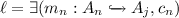
• $\exists (m,c)$ is a condition over a graph C, if is a mono and c is a condition over D,

• $\lnot c$ is a condition over C, if c is a condition over C, and

• $\wedge (c_1,\dots ,c_k)$ is a condition over C, if $c_1,\dots ,c_k$ are conditions over C.

A graph property is a condition over the empty graph $\emptyset$.

Note, the empty conjunction $\wedge ()$ serves as a base case for the inductive definition. Without extending expressiveness of the conditions, we define the following operators: $\vee (c_1,\dots , c_k)$:=$\lnot \wedge (\lnot c_1,\dots , \lnot c_k)$, $true$:=$\wedge ()$, $false$:=$\vee ()$, and $\forall (m,c)$:=$\lnot \exists (m,\lnot c)$. Finally, we also use $\wedge (S)$ if S is a finite set instead of a list.

Definition 2

(satisfaction). A graph mono satisfies a condition $\exists (m,c)$ where is a mono and where c is a condition over D, written $q\,\models \, \exists (m,c)$, if there is a mono  such that $q'\circ m=q$ and $q'\,\models \, c$. The satisfaction relation $\,\models \,$ is defined on the other connectives as expected. Finally, if G is a graph, p is a graph property, and the unique mono satisfies p, then G satisfies p, written $G\,\models \, p$.

Note that we reintroduced these definitions for graphs, but our results can be generalized to variants of graphs such as, e.g., typed attributed graphs, Petri nets, or even algebraic specifications, since they belong to an $\mathcal {M}$-adhesive category [6, 19] satisfying some additional categorical properties that the tableau-based reasoning method [20] requires. This is another advantage as opposed to using encodings as referred to in related work, since each kind of graph structure would otherwise need a different encoding.

Our symbolic model generation method will operate on the subset of conditions in conjunctive normal form (CNF), simplifying the corresponding reasoning. For example, $\wedge (\vee ()) =\wedge ( false )$ is a condition in CNF equivalent to $false$. We therefore assume an operation $[\cdot ]$, similarly to operations in [20, 25, 26], translating conditions into equivalent conditions in CNF. This operation applies, besides the expected equivalences, like the equivalence for removal of universal quantification mentioned before Definition 2, an equivalence for the removal of literals with isomorphisms (e.g., is replaced by by moving the isomorphism i into the literals of the next nesting level). In particular, a negative literal in CNF is trivially satisfiable by the identity morphism, a property that will be exploited heavily in our symbolic model generation algorithm. Note, skolemization, which removes existential quantification in FOL SAT-reasoning, is not needed for graph conditions [26, p. 100]; we employ CNF-conversion on quantified subconditions separately.

Definition 3

(CNF). A literal $\ell$ is either a positive literal $\exists (m,c)$ or a negative literal $\lnot \exists (m,c)$ where m is no isomorphism and c is in CNF. A clause is a disjunction of literals. A conjunction of clauses is a condition in CNF.

The tableau-based reasoning method as introduced in [20] is based on so-called nested tableaux. We start with reintroducing the notion of a regular tableau for a graph condition, which was directly inspired by the construction of tableaux for plain FOL reasoning [14]. Intuitively, provided a condition in CNF, such an iteratively constructed tableau represents all possible selections (computed using the extension rule in the following definition) of precisely one literal from each clause of the condition (note, a condition is unsatisfiable if it contains an empty clause). Such a selection is given by a maximal path in the tableau, which is called branch. In this sense, we are constructing a disjunctive normal form (DNF) where the set of nodes occurring in a branch of the resulting tableau corresponds to one clause of this DNF. Then, to discover contradictions in the literals of a branch and to prepare for the next step in the satisfiability analysis we merge (using the lift rule in the following definition) the selected literals into a single positive literal (note, if no positive literal is available the condition is always satisfiable), which is called opener. Note that the lift rule is based on a shifting translating a condition over a morphism into an equivalent condition [7, 13].

Definition 4

(tableau, tableau rules, open/closed branches). Given a condition c in CNF over C. A tableau T for c is a tree whose nodes are conditions constructed using the rules below. A branch in a tableau T for c is a maximal path in T. Moreover, a branch is closed if it contains $false$; otherwise, it is open. Finally, a tableau is closed if all of its branches are closed; otherwise, it is open.

• initialization rule: a tree with a single root node $true$ is a tableau for c.

• extension rule: if T is a tableau for c, B is a branch of T, and $\vee (c_1,\dots ,c_n)$ is a clause in c, then if $n>0$ and $c_1$, ..., $c_n$ are not in B, then extend B with n child nodes $c_1$, ..., $c_n$ or if $n=0$ and $false$ is not in B, then extend B with $false$.

• lift rule: if T is a tableau for c, B is a branch of T, $\exists (m,c')$ and $\ell$ are literals in B, $\ell '=\exists (m,[c' \wedge shift (m,\ell ) ])$ is not in B, then extend B with $\ell '$.

The operation $shift (\cdot ,\cdot )$ allows to shift conditions over morphisms preserving satisfaction in the sense that $m_1\circ m_2\,\models \, c$ iff $m_1\,\models \, shift (m_2,c)$ (see [20, Lemma 3]). Semi-saturated tableaux are the desired results of the iterative construction where no further rules need to be applied.

Definition 5

(semi-saturation, hook of a branch). Let T be a tableau for condition c over C. A branch B of T is semi-saturated if it is either closed or

• B is not extendable with a new node using the extension rule and

• if $E=\{\ell _1, \dots , \ell _n\}$ is nonempty and the set of literals added to B using the extension rule, then there is a positive literal $\ell =\exists (m,c')$ in E such that the literal in the leaf of B is equivalent to $\exists (m,c' \wedge _{\ell ' \in (E - \{\ell \})} shift (m,\ell '))$. Also, we call $\ell$ the hook of B.

Finally, T is semi-saturated if all its branches are semi-saturated.

In fact, a condition c is satisfiable if and only if the leaf condition of some open branch of a corresponding semi-saturated tableau is satisfiable. Hence, the next analysis step is required if there is a leaf of some open branch for which satisfiability has to be decided. That is, the next analysis step is to construct a tableau for condition $c'$. The iterative (possibly non-terminating) execution of this procedure results in (possibly infinitely many) tableaux where each tableau may result in the construction of a finite number of further tableaux. This relationship between a tableau and the tableaux derived from the leaf literals of open branches results in a so called nested tableau (see Fig. 2 for an example of a nested tableau).

Definition 6

(nested tableau, opener, context, nested branch, semi-saturation). Given a condition c over C and a poset $(I, \le , i_0)$ with minimal element $i_0$. A nested tableau $NT$ for c is for some $I'\subseteq I$ a family of triples $\{\langle T_i,j,c_i\rangle \}_{i \in I'}$ constructed using the following rules.

• initialization rule: If $T_{i_1}$ is a tableau for c, then the family containing only $\langle T_{i_1}, i_0, true \rangle$ for some index $i_1>i_0$ is a nested tableau for c and C is called context of $T_{i_1}$.

• nesting rule: If $NT$ is a nested tableau for c with index set $I'$, $\langle T_n,k,c_k\rangle$ is in $NT$ for index n, the literal is a leaf of $T_n$, $\ell$ is not the condition in any other triple of $NT$, $T_j$ is a tableau for $c_n$, and $j>n$ is some index not in $I'$, then add the triple $\langle T_j,n,\ell \rangle$ to $NT$ using index j, $\ell$ is called opener of $T_j$, and $A_j$ is called context of $T_j$.

A nested branch $NB$ of the nested tableau $NT$ is a maximal sequence of branches $B_{i_1},\dots ,B_{i_k},B_{i_{k+1}},\dots$ of tableaux $T_{i_1},\dots ,T_{i_k},T_{i_{k+1}},\dots$ in $NT$ starting with a branch $B_{i_1}$ in the initial tableau $T_{i_1}$ of $NT$, such that if $B_{i_{k}}$ and $B_{i_{k+1}}$ are consecutive branches in the sequence then the leaf of $B_{i_k}$ is the opener of $T_{i_{k+1}}$. $NB$ is closed if it contains a closed branch; otherwise, it is open. $NT$ is closed if all its nested branches are closed. Finally, $NT$ is semi-saturated if each tableau in $NT$ is semi-saturated.

Fig. 2.

Nested tableau (consisting of tableau $T_0$, ..., $T_5$) for graph property . In the middle branch $false$ is obtained because $\lnot \vee L_2$ is reduced to $false$ because $\vee L_2$ is reduced to $true$ because $L_2$ contains due to shifting, which is reduced by $[\cdot ]$ to $true$ because of the used isomorphism. We extract from the nested branches ending in $T_4$, $T_5$, and $T_3$ the symbolic models , , and . Here is a refinement of and, hence, would be removed by compaction as explained in Sect. 4.4.

It has been shown in [20] that the tableau based reasoning method using nested tableaux for conditions c is sound and refutationally complete. In particular, soundness means that if we are able to construct a nested tableau where all its branches are closed then the original condition c is unsatisfiable. Refutational completeness means that if a saturated tableau includes an open branch, then the original condition is satisfiable. In fact, each open finite or infinite branch in such a tableau defines a finite or infinite model of the property, respectively. Informally, the notion of saturation requires that all tableaux of the given nested tableau are semi-saturated and that hooks are selected in a fair way not postponing indefinitely the influence of a positive literal for detecting inconsistencies leading to closed nested branches.

4 Symbolic Model Generation

In this section we present our symbolic model generation algorithm. We first formalize the requirements from the introduction for the generated set of symbolic models, then present our algorithm, and subsequently verify that it indeed adheres to these formalized requirements. In particular, we want our algorithm to extract symbolic models from all open finite branches in a saturated nested tableau constructed for a graph property p. This would be relatively straightforward if each saturated nested tableau would be finite.

However, in general, as stated already at the end of the previous section this may not be the case. E.g., consider the conjunction $p_0=\wedge (p_1,p_2,p_3)$ of the conditions $p_1=$ (there is a node which has no predecessor), $p_2=$ (every node has a successor), and $p_3=$ (no node has two predecessors), which is only satisfied by the infinite graph $G_\infty =$

Thus, in order to be able to find a complete set of symbolic models without knowing beforehand if the construction of a saturated nested tableau terminates, we introduce the key-notions of k-semi-saturation and k-termination to reason about nested tableaux up to depth k, which are in some sense a prefix of a saturated tableau. Note, the verification of our algorithm, in particular for completeness, is accordingly based on induction on k. Informally, this means that by enlarging the depth k during the construction of a saturated nested tableau, we eventually find all finite open branches and thus finite models. This procedure will at the same time guarantee that we will be able to extract symbolic models from finite open branches even for the case of an infinite saturated nested tableau. E.g., we will be able to extract $\emptyset$ from a finite open branch of the infinite saturated nested tableau for property $p_4=$ .

4.1 Sets of Symbolic Models

The symbolic model generation algorithm $\mathcal {A}$ should generate for each graph property p a set of symbolic models $\mathcal {S}$ satisfying all requirements described in the introduction. A symbolic model in its most general form is a graph condition over a graph C, where C is available as an explicit component. A symbolic model then represents a possibly empty set of graphs (as defined subsequently in Definition 10). A specific set of symbolic models $\mathcal {S}$ for a graph property p satisfies the requirements soundness, completeness, minimal representability, and compactness if it adheres to the subsequent formalizations of these notions.

Definition 7

(symbolic model). If c is a condition over C according to Definition 1, then $\langle C,c\rangle$ is a symbolic model.

Based on the notion of m-consequence we relate symbolic models subsequently.

Definition 8

( m -consequence on conditions). If $c_1$ and $c_2$ are conditions over $C_1$ and $C_2$, respectively, is a mono, and for all monos and such that $m_2\circ m=m_1$ it holds that $m_2\,\models \, c_2$ implies $m_1\,\models \, c_1$, then $c_1$ is an m-consequence of $c_2$, written . We can state the existence of such an m by writing . We also omit m if it is the identity or clear from the context. Finally, conditions $c_1$ and $c_2$ over C are equivalent, written $c_1 \equiv c_2$, if and .

We define coverage of symbolic models based on the notion of m-refinement, which relies on an m-consequence between the contained conditions.

Definition 9

( m -refinement of symbolic model). If $\langle C_1,c_1\rangle$ and $\langle C_2,c_2\rangle$ are symbolic models and is a mono, and , then $\langle C_2,c_2\rangle$ is an m-refinement of $\langle C_1,c_1\rangle$, written . The set of all such symbolic models $\langle C_2,c_2\rangle$ is denoted by $refined (\langle C_1,c_1\rangle )$.

We define the graphs covered by a symbolic model as follows.

Definition 10

( m -covered by a symbolic model). If $\langle C,c\rangle$ is a symbolic model, G is a finite graph, is a mono, and $m\,\models \, c$ then G is an m-covered graph of $\langle C,c\rangle$. The set of all such graphs is denoted by $covered (\langle C,c\rangle )$. For a set $\mathcal {S}$ of symbolic models $covered (\mathcal {S}) =\cup _{s\in S} covered (s)$.

Based on these definitions, we formalize the first four requirements from Sect. 1 to be satisfied by the sets of symbolic models returned by algorithm $\mathcal {A}$.

Definition 11

(sound, complete, minimally representable, compact). Let $\mathcal {S}$ be a set of symbolic models and let p be a graph property. $\mathcal {S}$ is sound w.r.t. p if $covered (\mathcal {S}) \subseteq \{G\mid G\,\models \, p\wedge G~\text {is finite}\}$, $\mathcal {S}$ is complete w.r.t. p if $covered (\mathcal {S}) \supseteq \{G\mid G\,\models \, p\wedge G~\text {is finite}\}$, $\mathcal {S}$ is minimally representable w.r.t. p if for each $\langle C,c\rangle \in \mathcal {S}$: $C \,\models \, p$ and for each $G\in covered (\langle C,c\rangle )$ there is a mono , and $\mathcal {S}$ is compact if all $(s_1\ne s_2)\in \mathcal {S}$ satisfy $covered (s_1) \nsubseteq covered (s_1)$.

4.2 Symbolic Model Generation Algorithm $\mathcal {A}$

We briefly describe the two steps of the algorithm $\mathcal {A}$, which generates for a graph property p a set of symbolic models $\mathcal {A} (p)=\mathcal {S}$. The algorithm consists of two steps: the generation of symbolic models and the compaction of symbolic models, which are discussed in detail in Sects. 4.3 and 4.4, respectively. Afterwards, in Sect. 4.5, we discuss the explorability of the obtained set of symbolic models $\mathcal {S}$.

Step 1 (Generation of symbolic models in Sect. 4.3 ). We apply the tableau and nested tableau rules from Sect. 3 to iteratively construct a nested tableau. Then, we extract symbolic models from certain nested branches of this nested tableau that can not be extended. Since the construction of the nested tableau may not terminate due to infinite nested branches we construct the nested tableau in breadth-first manner and extract the symbolic models whenever possible. Moreover, we eliminate a source of nontermination by selecting the hook in each branch in a fair way not postponing the successors of a positive literal that was not chosen as a hook yet indefinitely [20, p. 29] ensuring at the same time refutational completeness of our algorithm. This step ensures that the resulting set of symbolic models is sound, complete (provided termination), and minimally representable. The symbolic models extracted from the intermediately constructed nested tableau $NT$ for growing k is denoted $\mathcal {S}_{ NT ,k}$.

Step 2 (Compaction of symbolic models in Sect. 4.4 ). We obtain the final result $\mathcal {S}$ from $\mathcal {S}_{ NT ,k}$ by the removal of symbolic model that are a refinement of any other symbolic model. This step preserves soundness (as only symbolic models are removed), completeness (as only symbolic models are removed that are refinements, hence, the removal does not change the set of covered graphs), and minimal representability (as only symbolic models are removed), and additionally ensures compactness.

4.3 Generation of $\mathcal {S}_{ NT ,k}$

By applying a breadth-first construction we build nested tableaux that are for increasing k, both, k-semi-saturated, stating that all branches occurring up to index k in all nested branches are semi-saturated, and k-terminated, stating that no nested tableau rule can be applied to a leaf of a branch occurring up to index k in some nested branch.

Definition 12

( k -semi-saturation, k -terminated). Given a nested tableau $NT$ for condition c over C. If $NB$ is a nested branch of length k of $NT$ and each branch B contained at index $i\le k$ in $NB$ is semi-saturated, then $NB$ is k-semi-saturated. If every nested branch of $NT$ of length n is $\mathop {min}(n,k)$-semi-saturated, then $NT$ is k-semi-saturated. If $NB$ is a nested branch of $NT$ of length n and the nesting rule can not be applied to the leaf of any branch B at index $i\le \mathop {min}(n,k)$ in $NB$, then $NB$ is k-terminated. If every nested branch of $NT$ of length n is $\mathop {min}(n,k)$-terminated, then $NT$ is k-terminated. If $NB$ is a nested branch of $NT$ that is k-terminated for each k, then $NB$ is terminated. If $NT$ is k-terminated for each k, then $NT$ is terminated.

We define the $k'$-remainder of a branch, which is a refinement of the condition of that tableau, that is used by the subsequent definition of the set of extracted symbolic models.

Definition 13

( $k'$ -remainder of branch). Given a tableau T for a condition c over C, a mono , a branch B of T, and a prefix P of B of length $k'>0$. If R contains (a) each condition contained in P unless it has been used in P by the lift rule (being $\exists (m,c')$ or $\ell$ in the lift rule in Definition 4) and (b) the clauses of c not used by the extension rule in P (being $\vee (c_1,\dots ,c_n)$ in the extension rule in Definition 4), then $\langle C,\wedge R \rangle$ is the k’-remainder of B.

The set of symbolic models extracted from a nested branch $NB$ is a set of certain $k'$-remainders of branches of $NB$. In the example given in Fig. 2 we extracted three symbolic models from the four nested branches of the nested tableau.

Definition 14

(extracted symbolic model). If $NT$ is a nested tableau for a condition c over C, $NB$ is a k-terminated and k-semi-saturated nested branch of $NT$ of length $n\le k$, B is the branch at index n of length $k'$ in $NB$, B is open, B contains no positive literals, then the k’-remainder of B is the symbolic model extracted from B. The set of all such extracted symbolic models from k-terminated and k-semi-saturated nested branches of $NT$ is denoted $\mathcal {S}_{ NT ,k}$.

Based on the previously introduced definitions of soundness, completeness, and minimal representability of sets of symbolic models w.r.t. graph properties we are now ready to verify the corresponding results on the algorithm $\mathcal {A}$.

Theorem 1

(soundness). If $NT$ is a nested tableau for a graph property p, then $\mathcal {S}_{ NT ,k}$ is sound w.r.t. p.

Theorem 2

(completeness). If $NT$ is a terminated nested tableau for a graph property p, k is the maximal length of a nested branch in $NT$, then $\mathcal {S}_{ NT ,k}$ is complete w.r.t. p.

As explained by the example at the beginning of Sect. 4 the algorithm may not terminate. However, the symbolic models extracted at any point during the construction of the nested tableau are a gradually extended underapproximation of the complete set of symbolic models. Moreover, the openers  of the branches that end nonterminated nested branches constitute an overapproximation by encoding a lower bound on missing symbolic models in the sense that each symbolic model that may be discovered by further tableau construction contains some $G_2$ as a subgraph.

Theorem 3

(minimal representability). If $NT$ is a nested tableau for a graph property p, then $\mathcal {S}_{ NT ,k}$ is minimally representable w.r.t p.

For $p_1\wedge p_2$ from Fig. 1 we obtain a terminated nested tableau (consisting of 114 tableaux with 25032 nodes) from which we generate 28 symbolic models (with a total number of 5433 negative literals in their negative remainders). For p from Fig. 2 we generate 3 symbolic models, which are given also in Fig. 2. In the next subsection we explain how to compact sets of symbolic models.

4.4 Compaction of $\mathcal {S}_{ NT ,k}$ into $\mathcal {S}$

The set of symbolic models $\mathcal {S}_{ NT ,k}$ as obtained in the previous section can be compacted by application of the following lemma. It states a sufficient condition for whether a symbolic model $\langle A_1,c_1\rangle$ refines another symbolic model $\langle A_2,c_2\rangle$, which is equivalent to $covered (\langle A_1,c_1\rangle ) \supseteq covered (\langle A_2,c_2\rangle )$. In this case we can remove the covered symbolic model $\langle A_2,c_2\rangle$ from $\mathcal {S}_{ NT ,k}$ without changing the graphs covered. Since the set of symbolic models $\mathcal {S}_{ NT ,k}$ is always finite we can apply the following lemma until no further coverages are determined.

Lemma 1

(compaction). If $\langle A_{1}, c_{1}\rangle$ and $\langle A_{2}, c_{2}\rangle$ are two symbolic models, is a mono, and $\exists (i_{2}, c_{2} \wedge \lnot shift (i_{2}, \exists (i_{1}, c_{1})))$ is not satisfiable by a finite graph, then covered$(\langle A_{1}, c_{1}\rangle ) \supseteq$ covered($\langle A_{2}, c_{2}\rangle$).

This lemma can be applied when we determine a mono m such that $\exists (i_2,c_2\wedge \lnot shift (i_2,\exists (i_1,c_1)) )$ is refutable. For this latter part we apply our tableau construction as well and terminate as soon as non-refutability is detected, that is, as soon as a symbolic model is obtained for the condition.

For the resulting set $\mathcal {S}$ of symbolic models obtained from iterated application of Lemma 1 we now state the compactness as defined before.

Theorem 4

(compactness). If $NT$ is a nested tableau for a graph property p, then $\mathcal {S} \subseteq \mathcal {S}_{ NT ,k}$ is compact.

For $p_1\wedge p_2$ from Fig. 1 we determined a single symbolic model with minimal model (given in Fig. 1e) that is contained by the minimal models of all 28 extracted symbolic models. However, this symbolic model covers only 2 of the other 27 symbolic models in the sense of Lemma 1. For p from Fig. 2 we removed one of the three symbolic models by compaction ending up with two symbolic models, which have incomparable sets of covered graphs as for the symbolic models remaining after compaction for $p_1\wedge p_2$ from Fig. 1.

4.5 Explorability of $\mathcal {S}$

We believe that the exploration of further graphs satisfying a given property p based on the symbolic models is often desireable. In fact, $covered (\mathcal {S})$ can be explored according to Definition 10 by selecting $\langle C,c\rangle \in \mathcal {S}$, by generating a mono to a new finite candidate graph G, and by deciding $m\,\models \, c$. Then, an entire automatic exploration can proceed by selecting the symbolic models $\langle C,c\rangle \in \mathcal {S}$ in a round-robin manner using an enumeration of the monos leaving C in each case. However, the exploration may also be guided interactively restricting the considered symbolic models and monos.

Fig. 3.

Two extension candidates that include the graph $G_0$ from Fig. 1e with obvious monos and .

For example, consider $p_2$ from Fig. 1c for which the algorithm $\mathcal {A}$ returns a single symbolic model $\langle G_0,c_0\rangle$ of which the minimal model is given in Fig. 1c. In an interactive exploration we may want to decide whether the two graphs given in Fig. 3 also satisfy $p_2$. In fact, because $m_1\,\models \, c_0$ and $m_2\not \,\models \, c_0$ we derive $G_1\,\models \, p_2$ and $G_2\not \,\models \, p_2$ as expected.

Fig. 4.

Implemented construction rules: $\ell$ is a literal, $\ell _s$ is a sequence of literals, L is a set of literals, $cl_i$ is a clause, and $\diamond$ is the unchanged value from the input.

5 Implementation

We implemented the algorithm $\mathcal {A}$ platform-independently using Java as our new tool AutoGraph using xsd-based [36] input/output-format.

For $p_1\wedge p_2$ from Fig. 1 we computed the symbolic models using AutoGraph in 7.4 s, 4.6 s, 3.4 s, 2.7 s, and 2.1 s using 1, 2, 3, 4, and 13 threads (machine: 256 GB DDR4, 2 $\times$ E5-2643 Xeon @ 3.4 GHz $\times$ 6 cores $\times$ 2 threads). The minimal models derived using AutoGraph for $p_1$, $p_2$, and $p_1\wedge p_2$ from Fig. 1 are given in Fig. 1d and e. For p from Fig. 2 AutoGraph terminates in negligable time.

While some elementary constructions used (such as computing CNF, existence of monos, and pair factorization) have exponential worst case executing time, we believe, based on our tool-based evaluation, that in many practical applications the runtime will be acceptable. Furthermore, we optimized performance by exploiting parallelizability of the tableaux construction (by considering each nested branch in parallel) and of the compaction of the sets of symbolic models (by considering each pair of symbolic models in parallel).

To limit memory consumption we discard parts of the nested tableau not required for the subsequent computation, which generates the symbolic models, as follows. The implemented algorithm operates on a queue (used to enforce the breadth-first construction) of configurations where each configuration represents the last branch of a nested branch of the nested tableau currently constructed (the parts of the nested tableau not given by theses branches are thereby not represented in memory). The algorithm starts with a single initial configuration and terminates if the queue of configurations is empty.

A configuration contains the information necessary to continue the further construction of the nested tableau (also ensuring fair selection of hooks) and to extract the symbolic models whenever one is obtained.

A configuration of the implementation is a tuple containing six elements $( inp , res , neg , q\text {-}pre , q\text {-}post , cm )$ where $inp$ is a condition c over C in CNF and is the remainder of the condition currently constructed (where clauses used already are removed), $res$ is $\bot$ or a positive literal into which the other literals from the branch are lifted, $neg$ is a list of negative literals over C from clauses already handled (this list is emptied as soon as a positive literal has been chosen for $res$), $q\text {-}pre$ is a queue of positive literals over C from which the first element is chosen for the $res$ component, $q\text {-}post$ is a queue of positive literals: once $res$ is a chosen positive literal we shift the elements from $q\text {-}pre$ over m to obtain elements of $q\text {-}post$, and $cm$ is the composition of the morphisms from the openers of the nested branch constructed so far and is used to obtain eventually symbolic models (if they exist).

Given a condition c over C the single initial configuration is $(c, \bot ,\lambda ,\lambda ,\lambda , id _{C})$. The implemented construction rules operating on these configurations are given in Fig. 4. Given a configuration c we check the rules in the order given for applicability and apply only the first rule found. For each rule, applicability is determined by the conditions above the line and each rule results in a set of configurations given below the rule.

Rule 1 stops further generation if the current result is unsatisfiable. Rule 2 ensures that hooks are selected from the queue (if the queue is not empty) to ensure fairness of hook selection. Rule 3 if the queue can not be used to select a hook and no clause remains, the nested branch is terminated and a symbolic model can be extracted by taking $\langle codomain ( cm ),\wedge neg \rangle$. Rule 4 implements the lifting rule (see Definition 4) for negative literals taken from $neg$. Rule 5 implements the lifting rule (see Definition 4) for positive literals taken from $q\text {-}pre$; if the morphism of the resulting positive literal is an isomorphism, as forbidden for literals in CNF, we move an equivalent condition in CNF into the current hook (also implementing the lift rule) instead of moving the literal to the queue $q\text {-}post$. Rule 6 implements the nesting rule (see Definition 6). Rule 7 deterministically implements the extension rule (see Definition 4) constructing for each literal of the first clause a new configuration to represent the different nested branches.

For soundness reconsider Definition 13 where the set R used in the condition $\wedge R$ recovers the desired information similarly to how it is captured in the configurations. The separation into different elements in the configurations then allows for queue handling and determinization.

6 Conclusion and Outlook

We presented a symbolic model generation procedure for graph properties being equivalent to FOL on graphs. Our algorithm is innovative in the sense that it is designed to generate a finite set of symbolic models that is sound, complete (upon termination), compact, minimally representable, and flexibly explorable. Moreover, the algorithm is highly parallelizable. The approach is implemented in a new tool, called AutoGraph.

As future work we aim at applying, evaluating, and optimizing our approach further w.r.t. different application scenarios from the graph database domain [37] as presented in this paper, but also to other domains such as model-driven engineering, where our approach can be used, e.g., to generate test models for model transformations [2, 11, 22]. We also aim at generalizing our approach to more expressive graph properties able to encode, e.g., path-related properties [21, 27, 28]. Finally, the work on exploration and compaction of extracted symbolic models as well as reducing their number during tableau construction is an ongoing task.

References

Bak, K., Diskin, Z., Antkiewicz, M., Czarnecki, K., Wasowski, A.: Clafer: unifying class and feature modeling. SoSyM 15(3), 811–845 (2016)
Baudry, B.: Testing model transformations: a case for test generation from input domain models. In: MDE4DRE (2009)
Beyhl, T., Blouin, D., Giese, H., Lambers, L.: On the operationalization of graph queries with generalized discrimination networks. In: [5], 170–186
Courcelle, B.: The expression of graph properties and graph transformations in monadic second-order logic. In: [31], 313–400
Echahed, R., Minas, M. (eds.): ICGT 2016. LNCS, vol. 9761. Springer, Cham (2016)
Ehrig, H., Ehrig, K., Prange, U., Taentzer, G.: Fundamentals of Algebraic Graph Transformation. Springer, Heidelberg (2006)
Ehrig, H., Golas, U., Habel, A., Lambers, L., Orejas, F.: \(\cal{M}\)-adhesive transformation systems with nested application conditions. part 2: embedding, critical pairs and local confluence. Fundam. Inform. 118(1–2), 35–63 (2012)
Ehrig, H., Golas, U., Habel, A., Lambers, L., Orejas, F.: \(\cal{M}\)-adhesive transformation systems with nested application conditions. part 1: parallelism, concurrency and amalgamation. Math. Struct. Comput. Sci. 24(4) (2014)
Erling, O., Averbuch, A., Larriba-Pey, J., Chafi, H., Gubichev, A., Prat-Pérez, A., Pham, M., Boncz, P.A.: The LDBC social network benchmark: interactive workload. In: Proceedings of the 2015 ACM SIGMOD International Conference on Management of Data, pp. 619–630. ACM (2015)
Gogolla, M., Hilken, F.: Model validation and verification options in a contemporary UML and OCL analysis tool. In: Modellierung 2016. LNI, vol. 254, pp. 205–220. GI (2016)
González, C.A., Cabot, J.: Test data generation for model transformations combining partition and constraint analysis. In: Ruscio, D., Varró, D. (eds.) ICMT 2014. LNCS, vol. 8568, pp. 25–41. Springer, Cham (2014). doi:10.1007/978-3-319-08789-4_3
Habel, A., Heckel, R., Taentzer, G.: Graph grammars with negative application conditions. Fundam. Inform. 26(3/4), 287–313 (1996)
Habel, A., Pennemann, K.: Correctness of high-level transformation systems relative to nested conditions. MSCS 19(2), 245–296 (2009)
Hähnle, R.: Tableaux and related methods. In: Handbook of Automated Reasoning (in 2 vols.), pp. 100–178 (2001)
Heckel, R., Wagner, A.: Ensuring consistency of conditional graph rewriting - a constructive approach. ENTCS 2, 118–126 (1995)
Jackson, E.K., Levendovszky, T., Balasubramanian, D.: Reasoning about metamodeling with formal specifications and automatic proofs. In: Whittle, J., Clark, T., Kühne, T. (eds.) MODELS 2011. LNCS, vol. 6981, pp. 653–667. Springer, Heidelberg (2011). doi:10.1007/978-3-642-24485-8_48
Jackson, E.K., Sztipanovits, J.: Constructive techniques for meta- and model-level reasoning. In: Engels, G., Opdyke, B., Schmidt, D.C., Weil, F. (eds.) MODELS 2007. LNCS, vol. 4735, pp. 405–419. Springer, Heidelberg (2007). doi:10.1007/978-3-540-75209-7_28
Krause, C., Johannsen, D., Deeb, R., Sattler, K., Knacker, D., Niadzelka, A.: An SQL-based query language and engine for graph pattern matching. In: Echahed and Minas [5], 153–169
Lack, S., Sobocinski, P.: Adhesive and quasiadhesive categories. ITA 39(3), 511–545 (2005)
Lambers, L., Orejas, F.: Tableau-based reasoning for graph properties. In: Giese, H., König, B. (eds.) ICGT 2014. LNCS, vol. 8571, pp. 17–32. Springer, Cham (2014). doi:10.1007/978-3-319-09108-2_2
Milicevic, A., Near, J.P., Kang, E., Jackson, D.: Alloy*: a general-purpose higher-order relational constraint solver. In: 37th IEEE/ACM International Conference on Software Engineering, ICSE 2015, vol. 1, pp. 609–619 (2015)
Mougenot, A., Darrasse, A., Blanc, X., Soria, M.: Uniform random generation of huge metamodel instances. In: Paige, R.F., Hartman, A., Rensink, A. (eds.) ECMDA-FA 2009. LNCS, vol. 5562, pp. 130–145. Springer, Heidelberg (2009). doi:10.1007/978-3-642-02674-4_10
Orejas, F., Ehrig, H., Prange, U.: Reasoning with graph constraints. Formal Asp. Comput. 22(3–4), 385–422 (2010)
Pennemann, K.: An algorithm for approximating the satisfiability problem of high-level conditions. ENTCS 213, 75–94 (2008)
Pennemann, K.-H.: Resolution-like theorem proving for high-level conditions. In: Ehrig, H., Heckel, R., Rozenberg, G., Taentzer, G. (eds.) ICGT 2008. LNCS, vol. 5214, pp. 289–304. Springer, Heidelberg (2008). doi:10.1007/978-3-540-87405-8_20
Pennemann, K.H.: Development of Correct Graph Transformation Systems, PhD Thesis. Dept. Informatik, Univ. Oldenburg (2009)
Poskitt, C.M., Plump, D.: Verifying monadic second-order properties of graph programs. In: Giese, H., König, B. (eds.) ICGT 2014. LNCS, vol. 8571, pp. 33–48. Springer, Cham (2014). doi:10.1007/978-3-319-09108-2_3
Radke, H.: Hr* graph conditions between counting monadic second-order and second-order graph formulas. ECEASST 61 (2013)
Radke, H., Arendt, T., Becker, J.S., Habel, A., Taentzer, G.: Translating essential OCL invariants to nested graph constraints focusing on set operations. In: Parisi-Presicce, F., Westfechtel, B. (eds.) ICGT 2015. LNCS, vol. 9151, pp. 155–170. Springer, Cham (2015). doi:10.1007/978-3-319-21145-9_10
Rensink, A.: Representing first-order logic using graphs. In: Ehrig, H., Engels, G., Parisi-Presicce, F., Rozenberg, G. (eds.) ICGT 2004. LNCS, vol. 3256, pp. 319–335. Springer, Heidelberg (2004). doi:10.1007/978-3-540-30203-2_23
Rozenberg, G. (ed.): Handbook of Graph Grammars and Computing by Graph Transformations. Foundations, vol. 1. World Scientific, Singapore (1997)
Salay, R., Chechik, M.: A generalized formal framework for partial modeling. In: Egyed, A., Schaefer, I. (eds.) FASE 2015. LNCS, vol. 9033, pp. 133–148. Springer, Heidelberg (2015). doi:10.1007/978-3-662-46675-9_9
Schneider, S., Lambers, L., Orejas, F.: Symbolic Model Generation for Graph Properties (Extended Version). No. 115 in Technische Berichte des Hasso-Plattner-Instituts für Softwaresystemtechnik an der Universität Potsdam, Universitätsverlag Potsdam, Hasso Plattner Institute (Germany, Potsdam), 1 edn. (2017)
Semeráth, O., Vörös, A., Varró, D.: Iterative and incremental model generation by logic solvers. In: Stevens, P., Wąsowski, A. (eds.) FASE 2016. LNCS, vol. 9633, pp. 87–103. Springer, Heidelberg (2016). doi:10.1007/978-3-662-49665-7_6
The Linked Data Benchmark Council (LDBC): Social network benchmark (2016). http://ldbcouncil.org/benchmarks/snb
T.W.W.W.C. (W3C): W3C xml schema definition language (xsd) 1.1 part 1: structures (2012)
Wood, P.T.: Query languages for graph databases. SIGMOD Rec. 41(1), 50–60 (2012)
Author information
Authors and Affiliations
Corresponding author
Editor information
Editors and Affiliations
Rights and permissions
Copyright information
© 2017 Springer-Verlag GmbH Germany
About this paper
Cite this paper
Schneider, S., Lambers, L., Orejas, F. (2017). Symbolic Model Generation for Graph Properties. In: Huisman, M., Rubin, J. (eds) Fundamental Approaches to Software Engineering. FASE 2017. Lecture Notes in Computer Science(), vol 10202. Springer, Berlin, Heidelberg. https://doi.org/10.1007/978-3-662-54494-5_13
Download citation
DOI: https://doi.org/10.1007/978-3-662-54494-5_13
Published:
Publisher Name: Springer, Berlin, Heidelberg
Print ISBN: 978-3-662-54493-8
Online ISBN: 978-3-662-54494-5
eBook Packages: Computer ScienceComputer Science (R0)